Computing marine plankton connectivity under thermal constraints

1 Introduction

Marine plankton inhabiting the sunlit ocean contribute to more than 50% of the global primary production, sequester atmospheric carbon in the ocean and sustain the marine food web (Falkowski, 1994; Field et al., 1998). A rich diversity and complex biogeography of plankton communities comprising of bacteria, phytoplankton and zooplankton in the ocean has been observed (Sournia et al., 1991; Simon et al., 2009; Ibarbalz et al., 2019). The drivers responsible for this distribution can be abiotic (e.g., ocean currents, temperature, nutrients) and biotic (e.g., predation and competition) and have been a focus of multiple studies (Dutkiewicz et al., 2020; Busseni et al., 2020; Laso-Jadart et al., 2021; Ward et al., 2021; Sommeria-Klein et al., 2021; Richter et al., 2022; Frémont et al., 2022). Plankton are generally non-motile and hence, mostly drift with the ocean currents. Advection is considered to be a primary factor in establishing plankton population structure across regions (White et al., 2010; McManus and Woodson, 2012; Wilkins et al., 2013; Hellweger et al., 2014; Doblin and van Sebille, 2016; Richter et al., 2022). Apart from major ocean currents, submesoscale structures like ocean fronts (Scotti and Pineda, 2007; Lévy et al., 2018) and pycnoclines (McManus and Woodson, 2012) also play a key role in accumulation and transport of plankton.

Over the recent decades, improvements in ocean models and observational data have led to development of approaches that study how well-connected oceanic regions are. Marine connectivity can either be studied using Lagrangian simulation of virtual particles with modelled ocean data or using real data from surface drifter trajectories. Since explicit simulations can be computationally expensive and drifters tend to accumulate over time, Markov transition matrices are advantageous to study connectivity on basin or global scale (van Sebille et al., 2012; van Sebille, 2014; van der Mheen et al., 2019; O’ Malley et al., 2021). To compute these matrices, the ocean is divided into grid cells and subsets of trajectories are used to compute transition of particle or drifter from one grid cell to another in a given time-step. Methods developed for connectivity have been applied to study water transport (Ser-Giacomi et al., 2015; McAdam and van Sebille, 2018; O’ Malley et al., 2021) and microscopic, drifting particles in the ocean like microplastic debris (Maximenko et al., 2012; van Sebille et al., 2012; Wichmann et al., 2019; van der Mheen et al., 2019) and plankton (Wilkins et al., 2013; van Sebille, 2014; Doblin and van Sebille, 2016; Jönsson and Watson, 2016; Ward et al., 2021; Trahms et al., 2021; Richter et al., 2022).

Some connectivity techniques have explored pathways that maximize the probability of connectivity between two regions as a consequence of major water transport routes (Ser-Giacomi et al., 2015; O’ Malley et al., 2021; Trahms et al., 2021; Drouin et al., 2022). These approaches have also been extended to plankton and larval dispersal (Trahms et al., 2021; Laso-Jadart et al., 2021). However, Jönsson and Watson (2016) advocated use of minimum time scales for plankton connectivity, stating that high plankton reproduction rates and that few organisms are sufficient to establish connectivity across regions even via a low-likelihood path. Applying minimum connectivity time approach, Jönsson and Watson (2016) observed decadal timescales for global plankton connectivity. In another study, Richter et al. (2022) find high correlation between minimum connectivity timescales of up to 1.5 years and plankton metagenomic dissimilarities between sampling stations. These studies have, however, only looked at plankton dispersal near the surface, whereas there are some plankton that drift below the surface and can even maintain their vertical depths.

Moreover, despite the role played by ocean currents, a major controlling factor to global plankton dispersal by currents is the ambient ocean temperature (Doblin and van Sebille, 2016; Ward et al., 2021). According to the metabolic theory of ecology (Brown et al., 2004), plankton growth and activity rates are governed by ambient temperature, slowly increasing with increasing temperature up to a threshold before falling. Consistent with the metabolic theory, studies have found that the plankton diversity across latitudinal gradients decreases towards the poles mainly driven by lower temperatures also referred to as Latitudinal Diversity Gradient (LDG) (Chust et al., 2013; Ibarbalz et al., 2019; Righetti et al., 2019). Studying monthly species distribution, Righetti et al. (2019) observed maximum species turnover at mid-latitudes (between ∼ 45^°N to 65^°N and near 45^°S) and the Arctic due to temperature variability with changing seasons. A recent meta-analysis of these thermal performance curves found that instead of a strict thermodynamic constraint, slightly hotter adaptation is more favorable for phytoplankton (Kontopoulos et al., 2020). Despite the possibility of some plankton species adapting to thermal changes (O’Donnell et al., 2018; Dam et al., 2021), global warming poses a threat to the existing plankton biogeography with cascading effects on the higher trophic levels (Henson et al., 2021). Studies suggest a poleward shift of some species and reduced diversity in the tropics (Thomas et al., 2012; Benedetti et al., 2021; Frémont et al., 2022). Hence, considering these thermal constraints can lead to an improved understanding of plankton connectivity in the ocean.

Here, we propose a connectivity approach for passively drifting plankton at different depths incorporating temperature analysis to ocean model simulations. We combine Lagrangian modelling with network theory to investigate the effect of different thermal constraints on plankton connectivity at the surface and subsurface between a set of sample locations in the Atlantic Ocean.

2 Method

2.1 Lagrangian simulations

In Lagrangian modelling, freely floating plankton can be represented by passively drifting virtual particles (van Sebille, 2014; Doblin and van Sebille, 2016). To model the plankton movement, we use the ocean current and temperature data from GLOB16 ocean model (based on Iovino et al. (2016)) run over a ten year period (2009 - 2018) specific to the Atlantic Ocean provided by Euro-Mediterranean Center on Climate Change (Figure 1). Daily field data is available on a C-grid with eddy-resolving spatial resolution of 1/16^°. We perform 2D numerical simulations of particles distributed across the Atlantic Ocean and adjacent polar regions using the open-source Lagrangian particle tracking framework Parcels (v2.3.1) (https://oceanparcels.org).

FIGURE 1

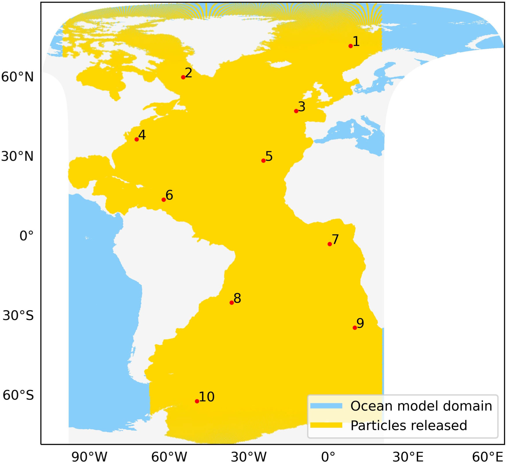
Figure 1 GLOB16 Ocean model data domain (in blue) and released particles (in yellow) along with locations of sample stations in the Atlantic Ocean (red points).

Release locations of virtual particles are defined using a hexagonal hierarchical geospatial indexing system called H3 (python library Version 3.7) developed by Uber (Brodsky, 2019). Hierarchical indexing provides unique identification to grid cells of different resolutions. At a given resolution, the H3 grid system offers approximately similar distance between centroids of neighbouring grid cells and similar grid cell area, whereas these values decrease as we move from the equator towards the poles in a latitude-longitude grid system. This advantage of the hexagonal grid system over latitude-longitude grid system have led to its use in recent connectivity studies (O’ Malley et al., 2021; Reijnders et al., 2021; Trahms et al., 2021).

We first get the centroids of all the hexagonal grids from resolution 5 of H3 between 100^°W to 20^°E. Resolution 5 provides a distance of ~ 16–18 km between each particle pair. Then, particles within the Atlantic Ocean are extracted using regional shapefiles from the Flanders Marine Institute (2021) and the remaining points present in the land mask of the model are removed. Thus, a final set of 375,570 particle release locations is used for all the simulations (yellow locations in Figure 1).

For each surface simulation using Parcels, particles are laterally advected with the horizontal velocities in the top layer (0 – 0.78 m) with 10 minutes time-step for a duration of one month i.e. 30 days using the fourth-order Runge-Kutta method. Particles are released on the 1st of each month and their positions after every 5 days along with minimum and maximum temperature observed by each particle are recorded in the output. Also, similar simulation set up is repeated at depths of 50, 100, 200 and 500 m to determine the effect of depth on plankton connectivity in the euphotic zone.

For demonstration purpose of the connectivity approach in this study, we use a set of 10 sample locations distributed across the Atlantic Ocean. These stations are well within the boundaries of the release domain (Figure 1) and representative of a broad range of thermal conditions. The exact locations are given in Table 1.

TABLE 1

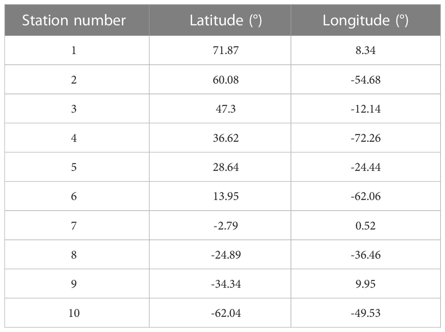
Table 1 Locations of sample stations in the Atlantic Ocean used in this study.

2.2 Connectivity analysis

Initial release and final positions of the particles from each simulation are first mapped to resolution 3 of the H3 system (Figure 2A). With resolution 3 of H3, each grid cell has approximately the same area as that of a 1°×1° (~ 111.2 km × 111.2 km) grid cell near the equator which has been found suitable for connectivity analysis previously (van Sebille et al., 2012; van Sebille, 2014; Smith et al., 2018; van der Mheen et al., 2019). In our study region, there are 8191 H3 resolution 3 grid cells in the Atlantic Ocean, with approximately 49 particles released per grid cell (minimum of 1 and maximum of 55 particles). Since we are interested in connectivity within the Atlantic Ocean, we only consider those particle transitions that end in the initial release domain 30 days after the release. Therefore, particles that exit the release domain boundaries or particles released below the bottom topography are ignored from further processing.

FIGURE 2

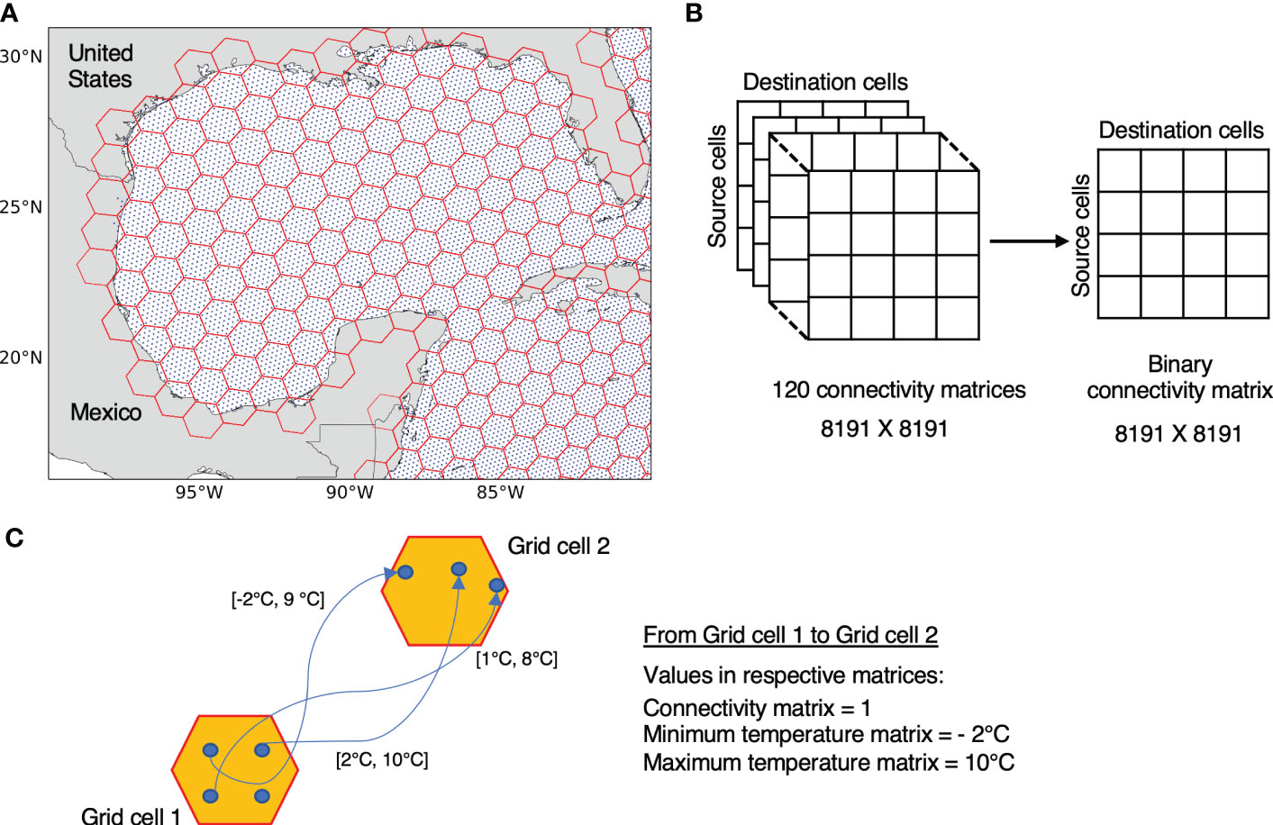
Figure 2 (A) Particles release and gridding shown for the Gulf of Mexico region: Particles release locations (in blue) are mapped to hexagonal cells (in red) using resolution 3 of H3 indexing system. (B) Presence or absence of connectivity between 8191 resolution 3 H3 grid cells across the release domain from 120 simulations are stored in a single binary matrix. (C) Extraction of resultant connectivity and minimum/maximum temperatures from multiple 30 days long trajectories connecting two grid cells. Values in square brackets represent the minimum and maximum temperature observed in a given particle trajectory.

We choose 30 days as the transition time-step dt. Previously, similar studies like van Sebille et al. (2012); van Sebille (2014); van der Mheen et al. (2019) have used dt of 2 months, primarily due to the uneven spread of drifters in the ocean which limits drifter transitions between grid cells (1^°×1^°) for time periods less than 60 days. Uniform release of virtual particles allows us to overcome this limitation for similar sized grid cells (H3 resolution 3) and majority (~88–90%) of the particles can establish cross-grid cell transition in 30 days. For smaller dt, for e.g., 5 days as used in O’ Malley et al. (2021), approximately half of the particles stay within their release grid cells. Therefore, dt of 30 days is representative of the time needed for the particles to perform cross grid-cell transport.

Presence and absence of particle transitions between source and destination grid cells from all the simulations is converted to a single binary matrix that we refer here onward as the connectivity matrix C of size 8191 × 8191 (8191 grid cells at H3 resolution 3), where rows represent the source, and columns the destination grid cells (Figure 2B). For extracting the temperatures, we make use of the minimum and maximum temperatures experienced by each particle along their trajectories during the 30 days of a given simulation. Note that multiple particles can connect the same pair of grid cells in a single simulation.

Let N denote the set of particles released and S denote the set of grid cells at a given H3 resolution. Let’s assume n particles (n ⊂ N) released at grid cell s end up in grid cell d from all the 30 days long simulations, where s, d ∈ S. Let minimum and maximum temperatures experienced by each particle be denoted by $min{T}_s^d$_p and $max{T}_s^d$_p respectively, where p denotes a given particle. The resultant minimum temperature ($Min{T}_s^d$) and maximum temperature ($Max{T}_s^d$) for connectivity from cell s to d are extracted from minimum and maximum temperatures observed by the n particles connecting s to d using (also see e.g. in Figure 2C):

$$Min{T}_s^d=\text{min}\left\{min{T}_{\mathrm{s 1}}^d,min{T}_{\mathrm{s 2}}^d,min{T}_{\mathrm{s 3}}^d,\dots ,min{T}_{\mathrm{s n}}^d\right\}$$

$$Max{T}_s^d=\text{max}\left\{max{T}_{\mathrm{s 1}}^d,max{T}_{\mathrm{s 2}}^d,max{T}_{\mathrm{s 3}}^d,\dots ,max{T}_{\mathrm{s n}}^d\right\}$$

The rationale for choosing minimum of minimum temperatures and maximum of maximum temperatures is discussed in Section 2.3. These minimum and maximum temperatures for each pair ($Min{T}_i^j$ $Max{T}_i^j \forall i,j\in N$) of connected grid cell are then stored in similar matrices (MinT and MaxT) as C.

2.2.1 Connectivity graph

A graph is the representation of a network where vertices are the different states of a system and edges define the relation between the vertices. We transform the connectivity matrix C into a directed and unweighted graph G using the graph-tool Python module (Peixoto, 2014). Here, we convert 8191 grid cells into vertices and existing transitions from source to destination grid cells into directed edges connecting the vertices of the graph. Minimum and maximum temperatures for the transitions are stored as the quantitative properties associated with the corresponding directed edges (Figure 3A).

FIGURE 3

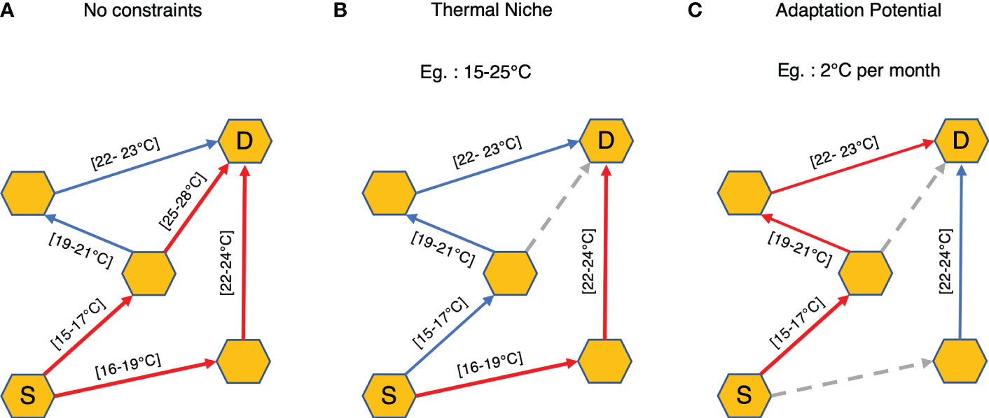
Figure 3 Schematic representations of different constraints applied on the connectivity graph G. Red arrows indicate the minimum connectivity time paths between Source cell (S) and Destination cell (D) for each case. Blue arrows represent the other valid transitions for the given scenario and dashed grey arrows are the dropped connections under the given constraints. Minimum and maximum temperatures for a given transition are provided in the square brackets beside the arrows. In case of (A) no thermal constraints, all the transitions are considered. For scenarios (B) Thermal Niche and (C) Adaptation Potential, transitions that do not conform to the constraints are discarded.

Similar to other marine connectivity related work (van Sebille et al., 2012; van Sebille, 2014; McAdam and van Sebille, 2018; van der Mheen et al., 2019; O’ Malley et al., 2021), we use Markov theory to study the transition of particles between grid cells. According to the Markovian assumption, given the current state in a system, the next state is independent of all the prior states. In our case, this is interpreted as a transition of particle from a given grid cell to another is independent of its past grid cells, where grid cells are the defined states of the system. Furthermore, the connectivity between grid cells is independent of the location where a particle enters or leaves a grid cell.

2.2.2 Minimum connectivity time

Taking motivation from Jönsson and Watson (2016), we compute paths with minimum travel time to assess connectivity between two grid cells. With this approach, we investigate the possible connectivity between grid cells, however likely or unlikely the pathways may be. Let $P_s^d$ be the set of possible pathways from source vertex (or grid cell) s to destination vertex d, where s, d, ∈ S. The set of minimum travel time paths between the vertices are then computed as:

$$MinimumTimePath{s}_s^d=\text{min}\left(P_s^d\right)$$

Breadth First Search (BFS) algorithm (Moore, 1959) implemented within the graph-tool library returns the shortest paths between two given vertices of the graph G. Note that algorithm can return zero to multiple paths, where zero path means absence of connectivity from s to d vertex. Each transition in a given shortest path is assigned the minimum time of 30 days (dt) and hence, the total number of transitions from source to destination gives the total travel time in months. In addition, we also perform two sensitivity analyses to test the robustness of the connectivity approach.

First, a bootstrap analysis is done to determine the effect of number of released particles used in the analysis. We create ensembles of different sizes of particles that are randomly selected without replacement from trajectories of each simulation. We use only surface simulation to perform this analysis. The connectivity matrix is then obtained from the selected particles only. The set of particle sizes tested for are 5,000, 10,000, 50,000, 100,000, 200,000 and 300,000. Bootstrap sampling for each particle size is done 100 times. Minimum connectivity paths and time are then compared for all the particle sizes, including the result from the full set of particles.

Secondly, we test the sensitivity of the surface connectivity to the choice of grid resolution. We compute connectivity matrices using resolution 2 (coarser, ~2.6^°near the equator) and 4 (finer, ~0.4^°near the equator) of H3 for mapping of released particles. The minimum connectivity time and paths then obtained from these resolutions are compared with results from resolution 3 of H3.

2.3 Species specific thermal constraints

Our main goal is to compute how the ocean temperature can constrain the plankton connectivity. We apply two types of thermal constraints, where connections that do not satisfy the constraints are filtered out from the matrix C before constructing the connectivity graph G. Hence, the graph we use for connectivity analysis is thermally constrained. Also, as shown in Section 2.2, we extract the widest range of temperatures ($Min{T}_s^d$ and $Max{T}_s^d$) for a connected grid cell pair from all simulations. This allows for exploration of possible pathways under a given temperature constraint within a broad range of temperatures acceptable to a plankton species.

1. Thermal niche: In ecology, a species preferred range of temperature which allows metabolic rates suitable for growth is called its thermal niche (Thomas et al., 2012). Here, we assume that the plankton can survive transport from one grid cell to another if its thermal niche overlaps at least partially with the minimum-maximum thermal range of the possible connections. Hence, all connections with thermal range outside the thermal niche of a given species are dropped from the graph G before computing the minimum travel time paths (Figure 3B).

2. Adaptation potential: Since plankton generally drift with the ocean currents, they also experience variations in temperature and can adapt or tolerate these changes to a certain extent (Doblin and van Sebille, 2016). Here, we use the word adaptation to refer to both adaptive evolution and acclimation. To estimate the influence of this adaptation efficiency on the connectivity, we keep only those transitions where the difference between the minimum and maximum temperature experienced by the plankton particle in a single transition (i.e., 30 days) doesn’t exceed a given value (Figure 3C).

Dropping of connections from the non-constrained connectivity matrix due to thermal constraints can lead to changes in the resultant minimum connectivity paths. As demonstrated in Figures 3B and C, the connectivity time can either remain the same or increase compared to the scenario without constraints, but never decrease (Figure 3A). In other cases, connectivity can also be lost if no pathways can be found between the interested stations.

Some plankton species with known thermal niche are foraminifera for e.g., Globigerinoides sacculifer (~ 18-29^°C) in the tropical waters and Globigerina bulloides (~5-26^°C) in the temperate to sub-tropical waters (Kucera, 2007) [their Figure 5], and cocolithophore Emiliania huxleyi (~ 2-27^°C) with a broad geographical domain (Fielding, 2013) For the technique demonstration, we make use of some sample constraints covering species types with narrow or wide thermal niche (TN TypeX) and higher or lower potential to adapt to specific range of changes in temperature in a given month (AP TypeX). Narrow thermal niche in cases of sample species TN Type1 (15-25^°C) represent a species preferring subtropical to temperate regions and TN Type2 (2-15^°C) subpolar to polar regions. TN Type3 (10-30^°C) represent a much broader thermal niche for a widely found species. There is lack of literature on adaptation potential rate. Calbet and Saiz (2022) observed selective advantage to marine plankton under thermal adaptation up to 3°C. Therefore, we test connectivity for 1, 2 and 3^°C of adaptation potential. The full list of these sample types are given in Table 2.

TABLE 2

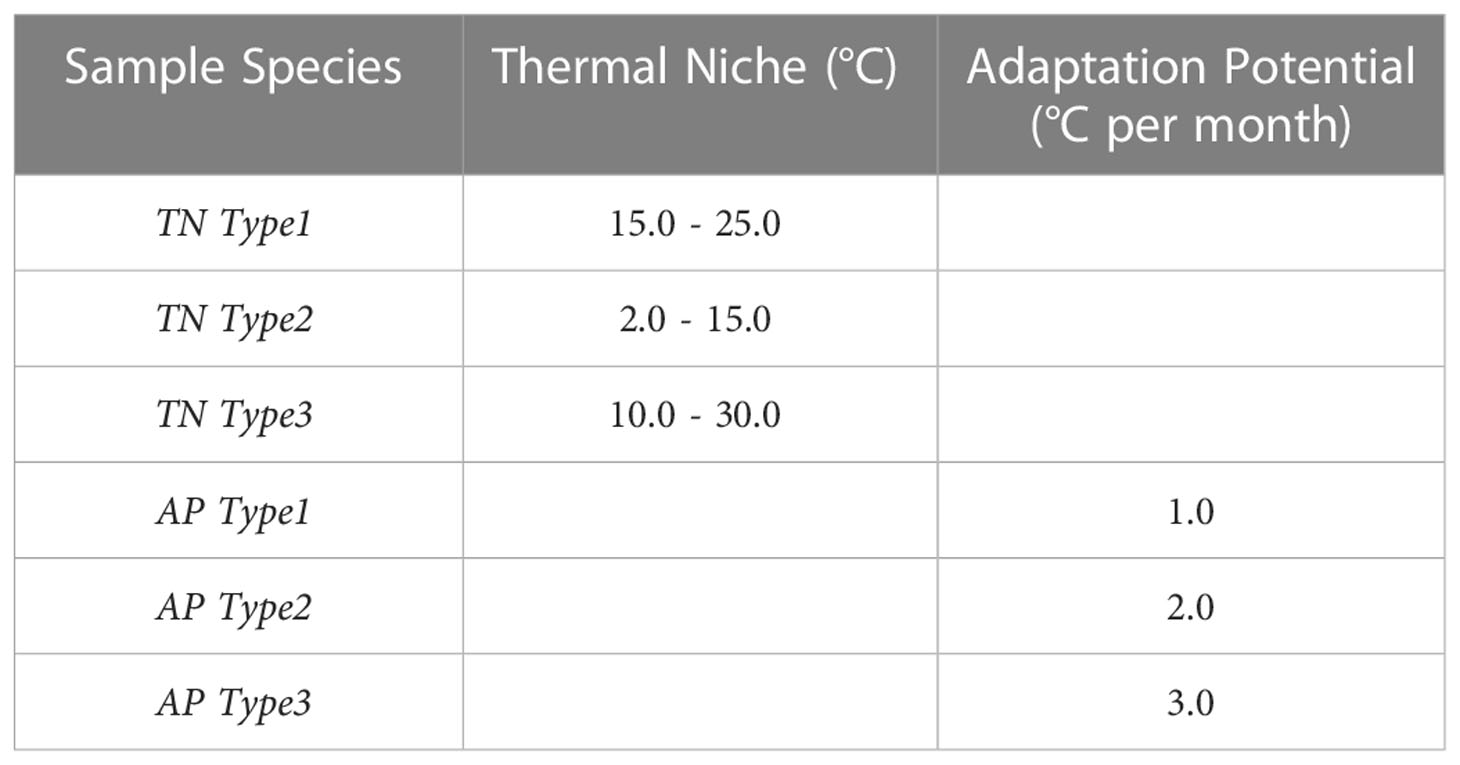
Table 2 The sample thermal constraints settings for which connectivity was computed in this study.

3 Results

3.1 General connectivity at the surface

Following previous studies (Jönsson and Watson, 2016; Richter et al., 2022), we estimate the minimum connectivity pathways for water parcels between sample stations (Figure 1). We find that all the stations can connect with other stations at the surface (Figure 4A). The white cell in Figure 4A from Station 7 to Station 7 connectivity corresponds to no connectivity within the grid cell containing Station 7. This can be attributed to the westward flowing South Equatorial Current (SEC) along this latitude (Figure 5). As expected, connectivity time in general increases with the distance between the stations. A maximum connectivity time of 2.67 years from Station 1 to Station 10 is observed. Figure 4A also suggests that stations in the South Atlantic can connect with stations in the North Atlantic in less time than vice-versa.

FIGURE 4

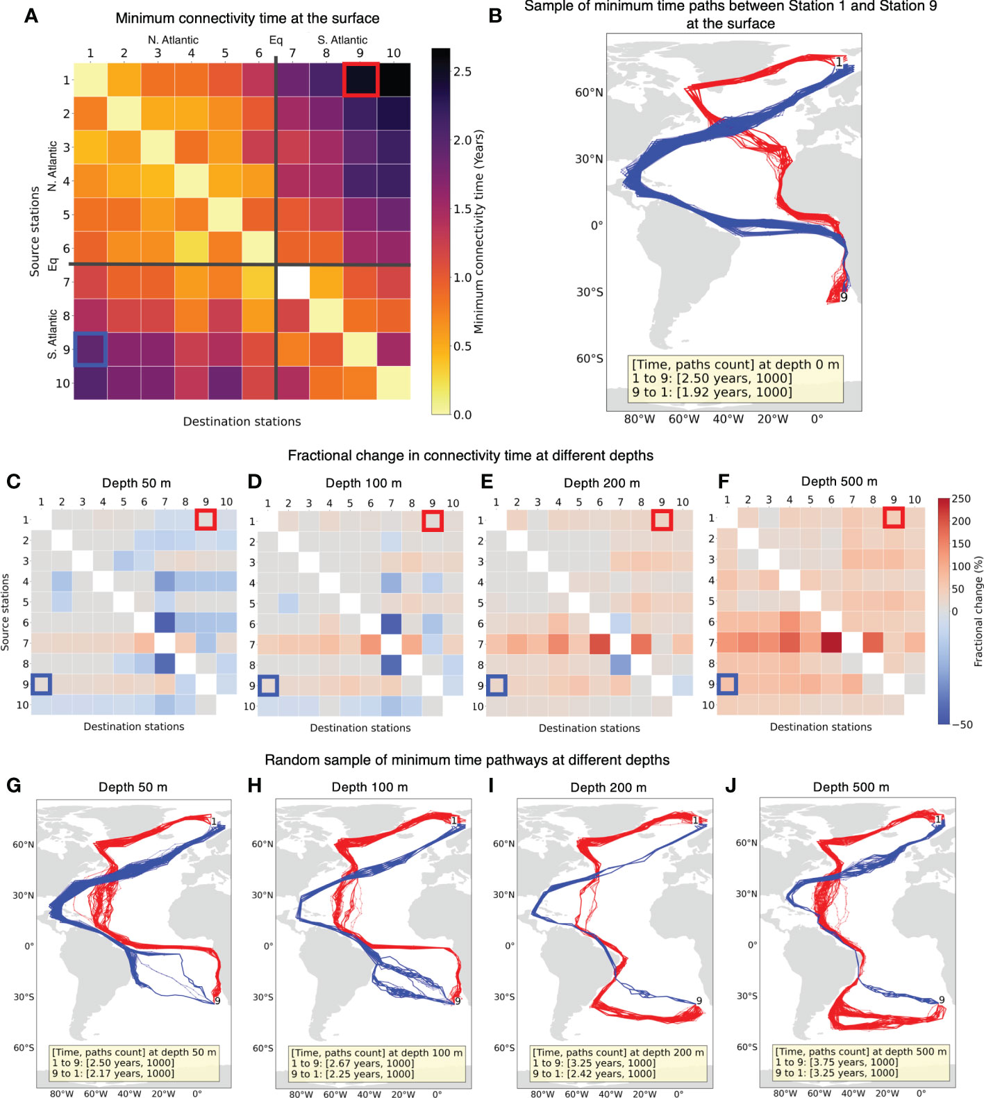
Figure 4 (A) Minimum connectivity time at the surface for non-constrained particles connecting source stations to destination stations. The stations are in the ascending order of their latitudes. (B) Example of random sample of minimum time connectivity paths at the surface between Station 1 and Station 9. Paths from Station 1 to 9 are indicated in red and from Station 9 to 1 are in blue. These paths are obtained by joining grid cell locations every 30 days, hence some paths may appear to cut across land. (C–F) The fractional change in connectivity time for depths 50, 100, 200 and 500 m, respectively compared to the surface connectivity time in (A). Colors in red tone indicate increase in connectivity time at a given depth while blue indicate decrease in connectivity time. (G–J) Random sample of minimum connectivity time pathways between the same two stations as (B) and depths same as the row above.

FIGURE 5

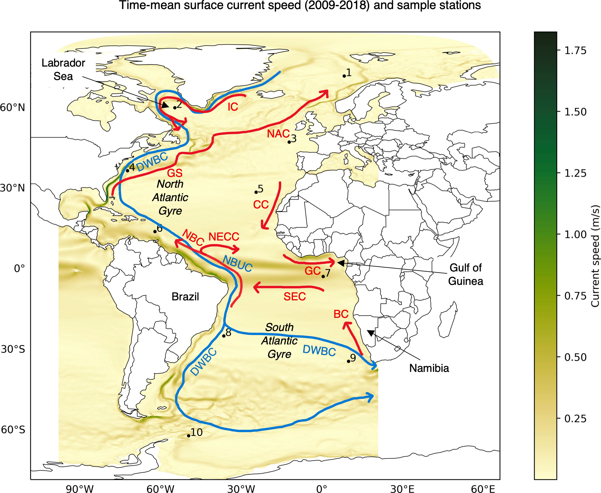
Figure 5 Time-mean of surface currents speed from GLOB16 Ocean data (2009-2018) and overview of surface (red) and deep (blue) currents adapted from Figure 1 of Bower et al. (2019). Sample station locations (Table 1) are also marked. BC: Benguela Current, CC: Canary Current, DWBC: Deep Western Boundary Current, GC: Guinea Current, GS: Gulf Stream, IC: Irminger Current, NAC: North Atlantic Current, NBC: North Brazil Current, NBUC: North Brazil Undercurrent, NECC: North Equatorial Counter Current, SEC: South Equatorial Current.

The connectivity between two stations in most cases yields multiple possible pathways with the same minimum connectivity time. An example of random sample of 1000 minimum connectivity time pathways between sample stations 1 and 9 situated in different hemispheres is shown in Figure 4B. Overall, the pathways in this example seem to mostly follow the major surface ocean currents (Bower et al., 2019). The paths from Station 1 (Figure 4B red trajectories) first go along the southern Greenland shelf and Labrador Sea via Irminger Current (IC), join the Canary Current (CC) near the north-western Africa to Gulf of Guinea via Guinea Current (GC) and then follow the west African coastline to arrive at Station 9 in 2.5 years (Figure 5). The average flow speeds along these paths is low from Station 1 to 9. On the other hand, paths from Station 9 (Figure 4B blue trajectories) trace along some of the fastest current systems of the Benguela Current (BC) flowing northward from the southern tip of Africa to connect with South Equatorial Current (SEC), North Brazil Current (NBC) along the slope of Brazil and Gulf Stream (GS) carrying warm water from the tropics that finally extends to the North Atlantic Current (NAC) to arrive at destination Station 1 in 1.92 years (Figure 5).

3.2 Connectivity at depths

We also compare the connectivity at the surface for water parcels (Figure 4A) with the connectivity at depths of 50, 100, 200 and 500 m. The connectivity time between station pairs generally increases as the depth increases which is expected due to decreasing current velocities at depths (Figures 4C–F). However, this increase in connectivity time is not monotonic. At 50 m depth, despite the expected decrease in flow speed, there is a decrease in connectivity time for many station pairs.

In Figures 4G-J, with a comparatively smaller change in connectivity time, large differences can be observed in the connectivity paths. We observe that from 50 m and deeper, connectivity paths are different when compared to the surface. The paths from Station 1 to 9 is along the Irminger Current (IC) crossing the North Atlantic Gyre to North Brazil Undercurrent (NBUC) and finally going east via the fast flowing North Equatorial Counter Current (NECC) (Figure 5) until 100 m depth and along the eastward flow of the Deep Western Boundary Current (DWBC) for depths of 200 and 500 m. For the reverse connectivity, the paths from Station 9 to Brazil traverse via the South Atlantic Gyre at depths and remaining routes across the equator from South Atlantic to the North Atlantic via North Brazil Current (NBC) and then up to Station 1 stay via Gulf Stream (GS) (Figure 5). We observe North Brazil Current (NBC) to be the main connectivity route from South Atlantic to North Atlantic at all the investigated depths (Figures 4B, G–J), which is responsible for the main northward transport of warm tropical water across the equator (Bower et al., 2019; Drouin et al., 2022).

3.3 Sensitivity analysis

3.3.1 Bootstrapping

We analyse the bootstrapping results from the surface simulations with an example pair of stations 1 and 9 (same as in Figure 4B). The minimum connectivity time obtained from 100 ensembles each from different particle set-size between the station pair (Figure 6A) show that for larger particle sets (>50,000) the timescales obtained are quite similar to the case of full particle set analysis. The connectivity paths for particles sets >50,000 also align well with the pathways in Figure 4B (Figures 6B, C). On the contrary, ensembles of smaller particle sets of 5,000 and 10,000 give higher connectivity time by up to 2 years and moreover, in some cases paths cannot be obtained (bar plots in Figure 6A). The connectivity paths from ensembles of smaller particle sets of 5,000 and 10,000 can be different than those in Figure 4B, causing connectivity time to increase by up to 2 years. Thus, the larger sets of particles show robust results and support our choice of number of particles.

FIGURE 6

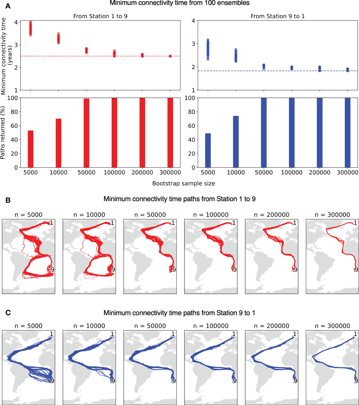
Figure 6 (A) Minimum connectivity time and (B–C) paths between Station 1 to 9 obtained from 100 bootstrap ensembles (surface simulations) each for different sample sizes. Red indicates connectivity from Station 1 to 9 and blue from Station 9 to 1. The bar plot in (A) represents the percentage of existing paths returned from the ensembles. The dashed horizontal lines represent minimum connectivity time from full set of 375,570 particles in respective cases, same as Figure 4B.

3.3.2 Grid resolution

Next, we compare the minimum connectivity results for H3 resolution 2 (1260 × 1260 matrix) and 4 (54,947 × 54,947 matrix) with results from resolution 3 (8191 × 8191 matrix). Finer resolution 5 of H3 was not tested due to intensive computational cost (with every increment in resolution, the size of the matrix increases approximately 7×7 times). Figure 7A shows that connectivity time decreases for coarser H3 resolution of 2, whereas, in Figure 7B, it increases for finer H3 resolution 4. To interpret this, note that we consider two grid cells connected when particles move from one cell to another in a period of 30 days (i.e., dt). However, this approach does not take into account the time it takes for a particle to move from one location to another within the same grid cell. Due to the Markovian assumption, the place where a connectivity path enters a grid cell is unrelated to the place where it then leaves the grid cell. Therefore, with larger grid cell sizes, faster connectivity can be achieved as it ignores the transport time within the grid cell itself. McAdam and van Sebille (2018) also found this artificial dispersion induced due to Markov modeling to be higher for larger grid size. Conversely, longer connectivity times can be expected with finer resolutions.

FIGURE 7

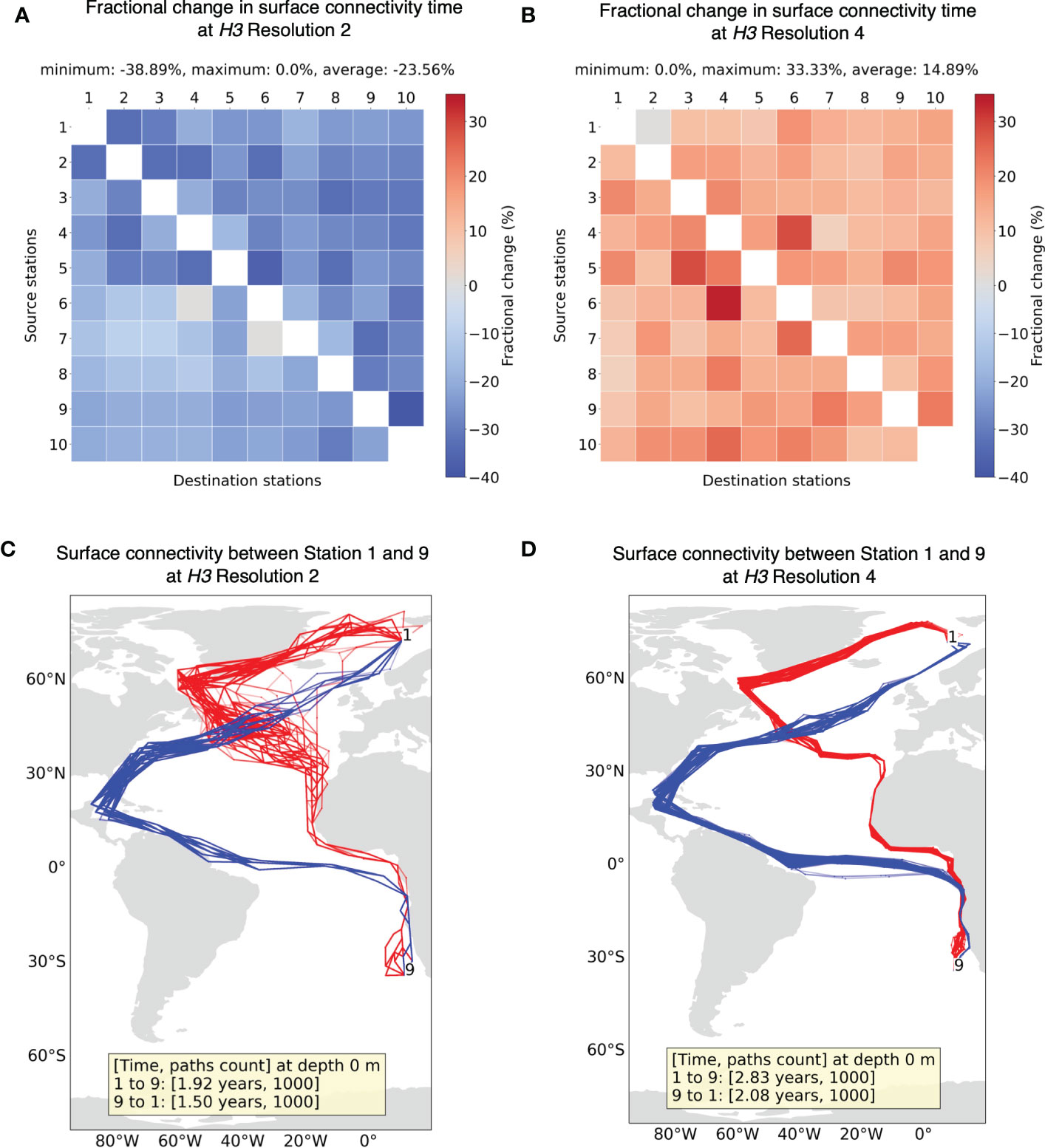
Figure 7 Fractional change in minimum connectivity time at the surface between all sample stations for (A) H3 resolution 2 and (B) H3 resolution 4 compared to the non-constrained surface connectivity time (Figure 4A). The stations are in the ascending order of their latitudes. Example of connectivity paths and time between Station 1 and 9 for (C) H3 resolution 2 and (D) H3 resolution 4.

For both resolutions 2 and 4, the sample of minimum connectivity paths between stations 1 and 9 (Figures 7C, D) seem to follow a similar profile to that of pathways from resolution 3 (Figure 4B). With resolution 2, certain segments of pathways appear quite narrow compared to higher resolutions, suggesting only selected cells allow connections between two distant regions. Although paths are quite similar for the three resolutions looked into, the effect of grid resolution on connectivity time must be taken into consideration in this approach.

3.4 Effects of thermal constraints

To test the different effects of thermal constraints on the connectivity, we apply the constraints from Table 2 on the connectivity graph at the surface and depth of 100 m. Again, we compare the fractional change in connectivity time for a given species type to the non-constrained connectivity time at the surface (Figure 4A). Also, a summary with maximum of the minimum connectivity times between all the sample stations comparing different constraint scenarios at the studied depths is provided in Table S1 of the Supplementary Material.

3.4.1 Thermal niche

Applying sample thermal niche constraints to the passive connectivity model, it is immediately clear (Figure 8) that the full surface connectivity breaks down – i.e., whether two stations are connected may depend on the chosen temperature range and depth. Limited by sea surface temperature and narrow thermal niche, species Type TN1 and Type TN2 (Figures 8A, B) can connect only a few pair of stations. We also observe loss of connectivity across the equator for species Type TN1 (Figure 8A) where only sub-tropical stations can establish connection within their respective hemispheres. For a cold-water species Type TN2, connectivity exists between four northernmost stations (Figure 8B). Despite that Station 10 may have favorable temperature for species Type TN2, it is unable to establish connection with other stations in the Southern Hemisphere which are in relatively warmer waters. On the other hand, a species with wide thermal niche like TN Type3 (Figure 8C) can establish connectivity across a larger domain. Only Station 2 is isolated from connectivity with other stations due to very low temperatures around the Labrador Sea. Even though being at a higher latitude than Station 2, Station 1 can establish connection with most of the stations due to warm surface water transported by the North Atlantic Current (NAC) (Bower et al., 2019). In general, we find an increase in connectivity time at the surface for all the species types, which is expected.

FIGURE 8

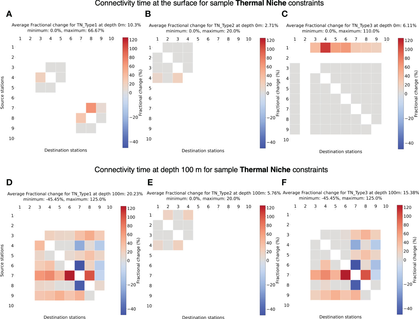
Figure 8 (A-C) Fractional change in minimum connectivity time at the surface compared to the non-constrained surface connectivity case in Figure 4A for sample thermal niches TN Type 1-3. (D-F) Fractional change in connectivity time at depth 100 m compared to the non-constrained surface connectivity case in Figure 4A for sample thermal niche constraints TN Type1-3. The details of these niches are listed in Table 2. The stations are in the ascending order of their latitudes.

At 100 m depth, connectivity for species TN Type1 connects more stations than at the surface and appears very similar to connectivity at 100 m for species TN Type3. However, compared to the surface, species TN Type3 is unable to connect with Station 1 due to lower temperatures at depth. TN Type3 showed similar connectivity as at the surface with marginal increase in connectivity time. Similar to the non-constrained connectivity scenarios (Figures 4C–F), the average connectivity time also increases compared to surface water connectivity due to lower flow speeds at depths, but can also decrease in certain cases likely due to change in paths.

3.4.2 Adaptation potential

For all the sample species types tested for adaptation potential (AP TypeX), we find an increase in connectivity timescales at the surface (Figures 9A–C). For a low adaptation potential of 1^°C per month (emphAP Type1), very few stations can establish connection with other stations at the surface (Figure 9A), which can be attributed to faster surface currents where temperatures can change quickly in a month’s time. In other cases of higher potential (AP Type2, AP Type3), the majority of the stations can establish connectivity.

FIGURE 9

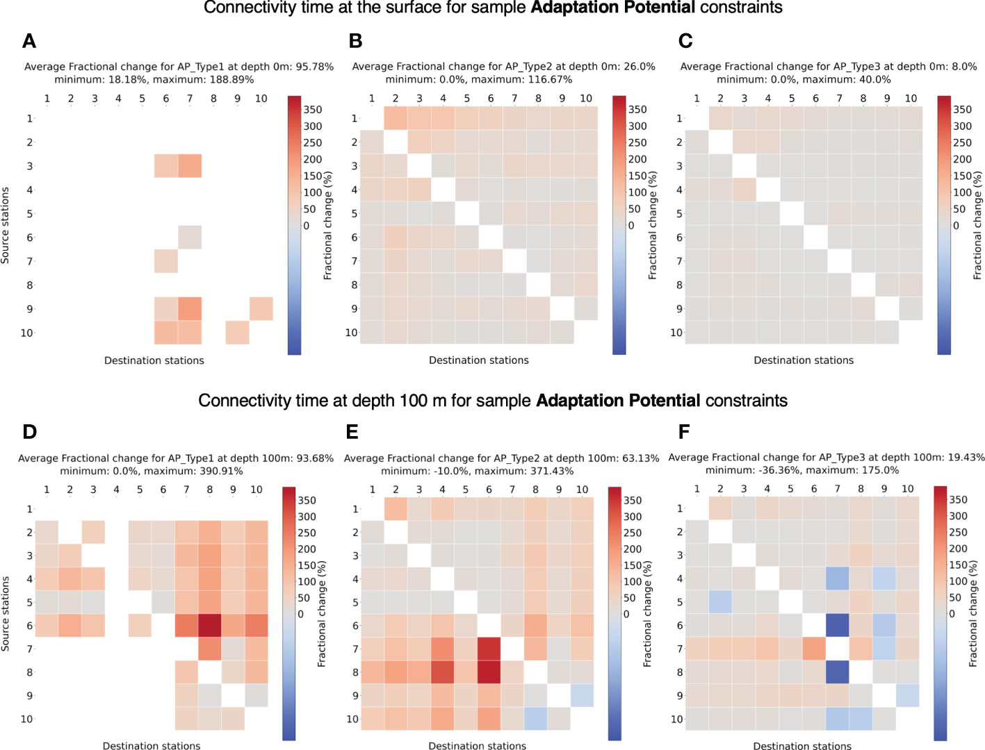
Figure 9 (A-C) Fractional change in minimum connectivity time at the surface compared to the non-constrained surface connectivity case in Figure 4A for sample adaptation potentials AP Type 1-3. (D-F) Fractional change in connectivity time at depth 100 m compared to the non-constrained surface connectivity case in Figure 4A for sample adaptation potentials AP Type 1-3. The details of these niches are listed in Table 2. The stations are in the ascending order of their latitudes.

At 100 m depth for AP Type1, most of the stations connect except from South Atlantic to North Atlantic (Figure 9D) likely due to average southward transport at depths (Bower et al., 2019), not allowing for slower changes in temperature. The increase in possible connectivity between stations at depths is expected as the temperature changes are smaller at depth. In the other cases of 2^°and 3^°C per month, most of the stations connect, both at surface (Figures 9B, C) and 100 m (Figures 9E, F) depth. Also, the increase in connectivity time at 100 m compared to the surface is clear given the lower current velocities.

4 Conclusion and discussion

In this paper, we propose a plankton connectivity approach using Lagrangian modeling and network theory techniques that particularly takes into account thermal tolerance of a plankton species and its habitable depths. We demonstrate how to compute the fastest possible pathways of connectivity using sample thermal constraints for a set of locations in the Atlantic Ocean. The same approach can also be used to study effects of other constraints to plankton dispersal like nutrients and salinity. In this method, we use a single connectivity matrix for the study region with minimum and maximum temperatures corresponding to the connections between grid cells. Therefore, we do not explore changes in connectivity with seasons, and rather aim to highlight the effects of thermal constraints on a general connectivity model already proposed by Jönsson and Watson (2016).

We use a similar approach as Jönsson and Watson (2016); Richter et al. (2022) to compute minimum connectivity for non-constrained particles (i.e., water parcels). As expected for non-constrained scenario, the method shows possible connectivity between all the sample stations both at the surface and at depth (Figures 4A, C–F). The minimum connectivity timescale obtained with our approach for surface water from Station 9 to 1 (Figure 4B) seem comparable, however, less than those from Figure 2H of Jönsson and Watson (2016) (note different source locations). We attribute these differences to differences in methodologies. Lower connectivity time in our case can be due to different particle seeding depths. We seed particles at the upper 1 m of the ocean surface, while Jönsson and Watson (2016) use velocities between 5 and 20 m below the surface (i.e., lower flow speeds compared to the surface). Conversely, larger grid size of 2^°×2^°in Jönsson and Watson (2016) can lead to faster connectivity time compared to ~ 1^°× 1^°in our study as also observed in Figure 7A. Some other differences that can affect the connectivity time computation are: (i) we use a higher resolution model of 1/16^°compared to 1/4^°in Jönsson and Watson (2016), (ii) differences in the ocean model data (NEMO vs ECCO2 and years used) and (iii) transition time-step dt is one month in our case while Jönsson and Watson (2016) used 3 days. Apart from this, as observed in O’ Malley et al. (2021), we also find clear influence of choice of grid resolution on connectivity time (Figures 7A, B). Therefore, we recommend interpreting connectivity time values using resolution 3 of H3 as relative time, where we focus on increase or decrease in connectivity time with respect to the connectivity for non-constrained particles at the surface.

In general, we find that the minimum connectivity pathways for water parcels reflect the major water transport routes via large-scale ocean currents. This is expected and it suggests that major ocean currents at respective depths can provide faster connectivity routes as seen in example pathways of Figures 4B, G–J, which correlate very well with upper and lower limbs of the Atlantic Meridional Overturning Circulation (AMOC) system discussed in Bower et al. (2019) [their Figure 1]. The North Brazil Current (NBC) is observed to be a bottleneck in northward connectivity routes from South Atlantic to North Atlantic (Figures 4B, G–J), as also observed in Bourlès et al. (1999); Bower et al. (2019); Drouin et al. (2022). However, it is also possible to have a segment or more of minimum connectivity pathways that can be against the large scale flow indicating possible connectivity via small scale oceanic features like eddies. For instance, in Figure 4B the paths from Station 1 to 9 (in red) near Namibia are opposite to the Benguela Current (BC). Also, an overall increase in connectivity time with increase in depth (Figures 4C–F) primarily correlates to decrease in flow speed over depth and possible changes in the connectivity pathways (Figure 4B, G–J).

Applying the sample thermal constraints (Table 2) to the connectivity, we observe that all the stations cannot establish connectivity creating subsets of connected stations under a given constraint (Figures 8, 9). The observed limitation imposed by thermal constraints of species niche corresponds well with observations made by Ward et al. (2021). In case of thermal niche constraints, the separation in connectivity between stations reflects the average temperature distribution at the ocean surface (Figure S1 in the Supplementary Material). This finding is aligned with Kucera (2007) [their Figure 5] where biogeography of planktonic foraminifera species is observed to correspond well with sea surface temperature. This suggests a potential use of this methodology to identify populations of a plankton species separated due to non-favorable temperature between regions. The effect of different sample thermal constraints is clearly visible on the connectivity. At the surface, species types with narrow thermal constraints (TN Type1, TN Type2 and AP Type1) clearly show limited connectivity (Figures 8A, B, 9A) compared to across basins connectivity possible for species with wider thermal constraints (TN Type3, AP Type2 and AP Type3) (Figures 8C, 9B, C). The increase in connectivity time for all the constraint types at the surface (Figures 8A-C, 9A-C) compared to the non-constrained connectivity at the surface indicates particles establishing connectivity using slightly longer paths to accommodate for thermal constraints.

Applying thermal constraints to dispersal at depths affects the connectivity variably depending on the constraints. For species TN Type1 and AP Type1 with narrow thermal constraints, more stations showed connectivity (even cross-equator connectivity) at depth 100 m (Figures 8D, 9D), while for TN Type3 with wide constraint, Station 1 is found to be isolated from other stations (Figure 8F) compared to the surface scenario (Figure 8C). These changes in connectivity are likely a consequence of lower ocean temperatures at depths and reduced current velocities. For other constraints (TN Type2, AP Type2 and AP Type3) possible connectivity between stations was not affected much (Figures 8E, 9E, F). Similar connectivities for adaptation potential of 2^°and 3^°C suggests possible rate of changes in temperature experienced by a particle in a month’s time in the ocean. The changes in connectivity time at depths for thermal constraints appear to have similar effect as that of Figure 4D, influenced by changes in connectivity paths and decreasing current speed.

Summarizing, the plankton connectivity methodology discussed in this paper provides an initial estimate of possible oceanographic connectivity and isolation between oceanic regions. This analysis can be combined with plankton genomic studies across a wide domain to develop an interdisciplinary approach and explore further the plankton biogeography. The role played by connectivity in interpretation of in-situ data has been emphasized by studies (Sommeria-Klein et al., 2021; Richter et al., 2022) investigating the genomic data collected from ocean-wide plankton samplings like Tara expeditions (Pesant et al., 2015; Ibarbalz et al., 2019; Sunagawa et al., 2020). This can be further examined with the proposed method for planktonic species with known thermal constraints for e.g.,foraminifera (Kucera, 2007). It can also be a potential tool to study future changes in plankton communities and distribution due to climate change. Indeed, there are some challenges in acquiring plankton thermal constraint data from the realenvironment and even laboratory experiments are limited and many times not viable for all species. As indicated, the connectivities obtained from this approach depend on the knowledge of the thermal niche or adaptation potential and floating depths of different plankton species. Hence, further sampling campaigns and physiological and genomic studies are encouraged.

Data availability statement

The datasets presented in this study can be found in online repositories. The code used for the study is available at: https://github.com/OceanParcels/atlanteco_tara_connectivity_plankton and the data generated at: https://doi.org/10.24416/UU01-HVXLB0. Ocean model data used in this study is accessible at https://doi.org/10.25424/cmcc/glob16-atlantic-2021.

Author contributions

Conceptualization of the study was done by DM, ES, LA-Z and DIu. Methodology was developed by DM and ES. DM performed the simulations, analysis, visualizations and wrote the original draft. Ocean model data was provided by DIo and SM. OJ, DIu, HS, LA-Z and ES contributed to the editing of the original draft. All authors contributed to manuscript revision, read, and approved the submitted version.

Funding

This project has received funding from the European Union’s Horizon 2020 research and innovation programme under grant agreement No. 862923. This output reflects only the author’s view, and the European Union cannot be held responsible for any use that may be made of the information contained therein.

Acknowledgments

The authors acknowledge the inputs and discussions from Fabio Benedetti (ETH, Zurich)

Conflict of interest

The authors declare that the research was conducted in the absence of any commercial or financial relationships that could be construed as a potential conflict of interest.

Publisher’s note

All claims expressed in this article are solely those of the authors and do not necessarily represent those of their affiliated organizations, or those of the publisher, the editors and the reviewers. Any product that may be evaluated in this article, or claim that may be made by its manufacturer, is not guaranteed or endorsed by the publisher.

Supplementary material

The Supplementary Material for this article can be found online at: https://www.frontiersin.org/articles/10.3389/fmars.2023.1066050/full#supplementary-material

References

Benedetti F., Vogt M., Elizondo U. H., Righetti D., Zimmermann N. E., Gruber N. (2021). Major restructuring of marine plankton assemblages under global warming. Nat. Commun. 12, 1–15. doi: 10.1038/s41467-021-25385-x

PubMed Abstract | CrossRef Full Text | Google Scholar

Bourlès B., Gouriou Y., Chuchla R. (1999). On the circulation in the upper layer of the western equatorial atlantic. J. Geophys. Res.: Oceans 104, 21151–21170. doi: 10.1029/1999JC900058

CrossRef Full Text | Google Scholar

Bower A., Lozier S., Biastoch A., Drouin K., Foukal N., Furey H., et al. (2019). Lagrangian Views of the pathways of the atlantic meridional overturning circulation. J. Geophys. Res.: Oceans 124, 5313–5335. doi: 10.1029/2019JC015014

CrossRef Full Text | Google Scholar

Brodsky I. (2019). H3: Uber's hexagonal hierarchical spatial index. h3-py python library v3.7.3.

PubMed Abstract | Google Scholar

Brown J. H., Gillooly J. F., Allen A. P., Savage V. M., West G. B. (2004). Toward a metabolic theory of ecology. Ecology 85, 1771–1789. doi: 10.1890/03-9000

CrossRef Full Text | Google Scholar

Busseni G., Caputi L., Piredda R., Fremont P., Hay Mele B., Campese L., et al. (2020). Large Scale patterns of marine diatom richness: Drivers and trends in a changing ocean. Global Ecol. Biogeogr. 29, 1915–1928. doi: 10.1111/geb.13161

CrossRef Full Text | Google Scholar

Calbet A., Saiz E. (2022). Thermal acclimation and adaptation in marine protozooplankton and mixoplankton. Front. Microbiol. 13. doi: 10.3389/fmicb.2022.832810

PubMed Abstract | CrossRef Full Text | Google Scholar

Chust G., Irigoien X., Chave J., Harris R. P. (2013). Latitudinal phytoplankton distribution and the neutral theory of biodiversity. Global Ecol. Biogeogr. 22, 531–543. doi: 10.1111/geb.12016

CrossRef Full Text | Google Scholar

Dam H. G., deMayo J. A., Park G., Norton L., He X., Finiguerra M. B., et al. (2021). Rapid, but limited, zooplankton adaptation to simultaneous warming and acidification. Nat. Climate Change 11, 780–786. doi: 10.1038/s41558-021-01131-5

CrossRef Full Text | Google Scholar

Dataset Flanders Marine Institute (2021). Global oceans and seas, version 1. Available at: https://www.marineregions.org/.

Google Scholar

Doblin M. A., van Sebille E. (2016). Drift in ocean currents impacts intergenerational microbial exposure to temperature. Proc. Natl. Acad. Sci. 113, 5700–5705. doi: 10.1073/pnas.1521093113

CrossRef Full Text | Google Scholar

Drouin K. L., Lozier M. S., Beron-Vera F. J., Miron P., Olascoaga M. J. (2022). Surface pathways connecting the south and north atlantic oceans. Geophys. Res. Lett. 49, e2021GL096646. doi: 10.1029/2021GL096646

CrossRef Full Text | Google Scholar

Dutkiewicz S., Cermeno P., Jahn O., Follows M. J., Hickman A. E., Taniguchi D. A., et al. (2020). Dimensions of marine phytoplankton diversity. Biogeosciences 17, 609–634. doi: 10.5194/bg-17-609-2020

CrossRef Full Text | Google Scholar

Falkowski P. G. (1994). The role of phytoplankton photosynthesis in global biogeochemical cycles. Photosynthesis Res. 39, 235–258. doi: 10.1007/BF00014586

CrossRef Full Text | Google Scholar

Field C. B., Behrenfeld M. J., Randerson J. T., Falkowski P. (1998). Primary production of the biosphere: integrating terrestrial and oceanic components. Science 281, 237–240. doi: 10.1126/science.281.5374.237

PubMed Abstract | CrossRef Full Text | Google Scholar

Fielding S. R. (2013). Emiliania huxleyi specific growth rate dependence on temperature. Limnology Oceanogr. 58, 663–666. doi: 10.4319/lo.2013.58.2.0663

CrossRef Full Text | Google Scholar

Frémont P., Gehlen M., Vrac M., Leconte J., Delmont T. O., Wincker P., et al. (2022). Restructuring of plankton genomic biogeography in the surface ocean under climate change. Nat. Climate Change 12, 393–401. doi: 10.1038/s41558-022-01314-8

CrossRef Full Text | Google Scholar

Hellweger F. L., van Sebille E., Fredrick N. D. (2014). Biogeographic patterns in ocean microbes emerge in a neutral agent-based model. Science 345, 1346–1349. doi: 10.1126/science.1254421

PubMed Abstract | CrossRef Full Text | Google Scholar

Henson S. A., Cael B., Allen S. R., Dutkiewicz S. (2021). Future phytoplankton diversity in a changing climate. Nat. Commun. 12, 1–8. doi: 10.1038/s41467-021-25699-w

PubMed Abstract | CrossRef Full Text | Google Scholar

Ibarbalz F. M., Henry N., Brandão M. C., Martini S., Busseni G., Byrne H., et al. (2019). Global trends in marine plankton diversity across kingdoms of life. Cell 179, 1084–1097. doi: 10.1016/j.cell.2019.10.008

PubMed Abstract | CrossRef Full Text | Google Scholar

Iovino D., Masina S., Storto A., Cipollone A., Stepanov V. N. (2016). A 1/16 eddying simulation of the global nemo sea-ice–ocean system. Geoscientific Model. Dev. 9, 2665–2684. doi: 10.5194/gmd-9-2665-2016

CrossRef Full Text | Google Scholar

Jönsson B. F., Watson J. R. (2016). The timescales of global surface-ocean connectivity. Nat. Commun. 7, 1–6. doi: 10.1038/ncomms11239

CrossRef Full Text | Google Scholar

Kontopoulos D.-G., van Sebille E., Lange M., Yvon-Durocher G., Barraclough T. G., Pawar S. (2020). Phytoplankton thermal responses adapt in the absence of hard thermodynamic constraints. Evolution 74, 775–790. doi: 10.1111/evo.13946

PubMed Abstract | CrossRef Full Text | Google Scholar

Kucera M. (2007). Chapter six planktonic foraminifera as tracers of past oceanic environments. Developments Mar. Geol. 1, 213–262. doi: 10.1016/S1572-5480(07)01011-1

CrossRef Full Text | Google Scholar

Laso-Jadart R., O’Malley M., Sykulski A., Ambroise C., Madoui M.-A. (2021). How marine currents and environment shape plankton genomic differentiation: a mosaic view from Tara oceans metagenomic data. doi: 10.1101/2021.04.29.441957

PubMed Abstract | CrossRef Full Text | Google Scholar

Lévy M., Franks P. J., Smith K. S. (2018). The role of submesoscale currents in structuring marine ecosystems. Nat. Commun. 9, 1–16. doi: 10.1038/s41467-018-07059-3

PubMed Abstract | CrossRef Full Text | Google Scholar

Maximenko N., Hafner J., Niiler P. (2012). Pathways of marine debris derived from trajectories of lagrangian drifters. Mar. pollut. Bull. 65, 51–62. doi: 10.1016/j.marpolbul.2011.04.016

PubMed Abstract | CrossRef Full Text | Google Scholar

McAdam R., van Sebille E. (2018). Surface connectivity and interocean exchanges from drifter-based transition matrices. J. Geophys. Res.: Oceans 123, 514–532. doi: 10.1002/2017JC013363

PubMed Abstract | CrossRef Full Text | Google Scholar

McManus M. A., Woodson C. B. (2012). Plankton distribution and ocean dispersal. J. Exp. Biol. 215, 1008–1016. doi: 10.1242/jeb.059014

CrossRef Full Text | Google Scholar

Moore E. F. (1959). “The shortest path through a maze,” in Proceedings of an international symposium on the theory of switching, part II (Cambridge, MA: Harvard University Press), 285–292.

Google Scholar

O’Donnell D. R., Hamman C. R., Johnson E. C., Kremer C. T., Klausmeier C. A., Litchman E. (2018). Rapid thermal adaptation in a marine diatom reveals constraints and trade-offs. Global Change Biol. 24, 4554–4565. doi: 10.1111/gcb.14360

CrossRef Full Text | Google Scholar

O’ Malley M., Sykulski A. M., Laso-Jadart R., Madoui M.-A. (2021). Estimating the travel time and the most likely path from lagrangian drifters. J. Atmospheric Oceanic Technol. 38, 1059–1073. doi: 10.1175/JTECH-D-20-0134.1

CrossRef Full Text | Google Scholar

Peixoto T. P. (2014). The graph-tool python library. Figshare. doi: 10.6084/m9.figshare.1164194

CrossRef Full Text | Google Scholar

Pesant S., Not F., Picheral M., Kandels-Lewis S., Le Bescot N., Gorsky G., et al. (2015). Open science resources for the discovery and analysis of tara oceans data. Sci. Data 2, 1–16. doi: 10.1038/sdata.2015.23

CrossRef Full Text | Google Scholar

Reijnders D., van Leeuwen E. J., van Sebille E. (2021). Ocean surface connectivity in the arctic: Capabilities and caveats of community detection in lagrangian flow networks. J. Geophys. Res.: Oceans 126, e2020JC016416. doi: 10.1029/2020JC016416

PubMed Abstract | CrossRef Full Text | Google Scholar

Richter D. J., Watteaux R., Vannier T., Leconte J., Frémont P., Reygondeau G., et al. (2022). Genomic evidence for global ocean plankton biogeography shaped by large-scale current systems. eLife 11, e78129. doi: 10.7554/eLife.78129.sa2

PubMed Abstract | CrossRef Full Text | Google Scholar

Righetti D., Vogt M., Gruber N., Psomas A., Zimmermann N. E. (2019). Global pattern of phytoplankton diversity driven by temperature and environmental variability. Sci. Adv. 5, eaau6253. doi: 10.1126/sciadv.aau6253

CrossRef Full Text | Google Scholar

Scotti A., Pineda J. (2007). Plankton accumulation and transport in propagating nonlinear internal fronts. J. Mar. Res. 65, 117–145. doi: 10.1357/002224007780388702

CrossRef Full Text | Google Scholar

Ser-Giacomi E., Vasile R., Hernandez-Garcia E., López C. (2015). Most probable paths in temporal weighted networks: An application to ocean transport. Phys. Rev. E 92, 012818. doi: 10.1103/PhysRevE.92.012818

CrossRef Full Text | Google Scholar

Simon N., Cras A.-L., Foulon E., Lemée R. (2009). Diversity and evolution of marine phytoplankton. Comptes Rendus Biol. 332, 159–170. doi: 10.1016/j.crvi.2008.09.009

CrossRef Full Text | Google Scholar

Smith T. M., York P. H., Broitman B. R., Thiel M., Hays G. C., van Sebille E., et al. (2018). Rare long-distance dispersal of a marine angiosperm across the pacific ocean. Global Ecol. Biogeogr. 27, 487–496. doi: 10.1111/geb.12713

CrossRef Full Text | Google Scholar

Sommeria-Klein G., Watteaux R., Ibarbalz F. M., Pierella Karlusich J. J., Iudicone D., Bowler C., et al. (2021). Global drivers of eukaryotic plankton biogeography in the sunlit ocean. Science 374, 594–599. doi: 10.1126/science.abb3717

PubMed Abstract | CrossRef Full Text | Google Scholar

Sournia A., Chrétiennot M.-J., Ricard M. (1991). Marine phytoplankton: how many species in the world ocean? J. Plankton Res. 13, 1093–1099. doi: 10.1093/plankt/13.5.1093

CrossRef Full Text | Google Scholar

Sunagawa S., Acinas S. G., Bork P., Bowler C., Eveillard D., Gorsky G., et al. (2020). Tara Oceans: towards global ocean ecosystems biology. Nat. Rev. Microbiol. 18, 428–445. doi: 10.1038/s41579-020-0364-5

PubMed Abstract | CrossRef Full Text | Google Scholar

Thomas M. K., Kremer C. T., Klausmeier C. A., Litchman E. (2012). A global pattern of thermal adaptation in marine phytoplankton. Science 338, 1085–1088. doi: 10.1126/science.1224836

PubMed Abstract | CrossRef Full Text | Google Scholar

Trahms C., Handmann P., Rath W., Visbeck M., Renz M. (2021). “Where have all the larvae gone? towards fast main pathway identification from geospatial trajectories,” in 17th international symposium on spatial and temporal databases (New York, NY, USA: Association for Computing Machinery), 126–129. SSTD ’21. doi: 10.1145/3469830.3470896

CrossRef Full Text | Google Scholar

van der Mheen M., Pattiaratchi C., van Sebille E. (2019). Role of indian ocean dynamics on accumulation of buoyant debris. J. Geophys. Res.: Oceans 124, 2571–2590. doi: 10.1029/2018JC014806

CrossRef Full Text | Google Scholar

van Sebille E. (2014). Adrift. org. au—a free, quick and easy tool to quantitatively study planktonic surface drift in the global ocean. J. Exp. Mar. Biol. Ecol. 461, 317–322. doi: 10.1016/j.jembe.2014.09.002

CrossRef Full Text | Google Scholar

van Sebille E., England M. H., Froyland G. (2012). Origin, dynamics and evolution of ocean garbage patches from observed surface drifters. Environ. Res. Lett. 7, 044040. doi: 10.1088/1748-9326/7/4/044040

CrossRef Full Text | Google Scholar

Ward B. A., Cael B., Collins S., Young C. R. (2021). Selective constraints on global plankton dispersal. Proc. Natl. Acad. Sci. 118, e2007388118. doi: 10.1073/pnas.2007388118

CrossRef Full Text | Google Scholar

White C., Selkoe K. A., Watson J., Siegel D. A., Zacherl D. C., Toonen R. J. (2010). Ocean currents help explain population genetic structure. Proc. R. Soc. B: Biol. Sci. 277, 1685–1694. doi: 10.1098/rspb.2009.2214

CrossRef Full Text | Google Scholar

Wichmann D., Delandmeter P., Dijkstra H. A., van Sebille E. (2019). Mixing of passive tracers at the ocean surface and its implications for plastic transport modelling. Environ. Res. Commun. 1, 115001. doi: 10.1088/2515-7620/ab4e77

CrossRef Full Text | Google Scholar

Wilkins D., van Sebille E., Rintoul S. R., Lauro F. M., Cavicchioli R. (2013). Advection shapes southern ocean microbial assemblages independent of distance and environment effects. Nat. Commun. 4, 1–7. doi: 10.1038/ncomms3457

CrossRef Full Text | Google Scholar