Recommendations for the design of in situ sampling strategies to reconstruct fine-scale ocean currents in the context of SWOT satellite mission

1 Introduction

Satellite observations of sea surface height (SSH) have enhanced our understanding of the global ocean large and mesoscale circulation over the last few decades (e.g., Chelton et al., 2011). Altimetric gridded products built from satellite measurements provide daily maps of SSH with a mean effective spatial resolution of ~200 km wavelength for the global ocean at mid-latitudes and ~130 km for the Mediterranean Sea (Ballarotta et al., 2019). The launch of the new Surface Water and Ocean Topography (SWOT) satellite mission conducted in December 2022 is considered a major advance in satellite ocean observation (Morrow et al., 2019). The SWOT mission is expected to provide SSH observations in two dimensions along a wide-swath altimeter track with an effective resolution down to 15-30 km wavelength, one order of magnitude higher than present altimeters (Fu and Ferrari, 2008; Fu and Ubelmann, 2014; Wang et al., 2019). After launch, the SWOT satellite is following a fast-sampling orbit to provide daily measurements of SSH in specific areas of the world ocean for instrumental calibration and validation.

Fine-scales are defined in the altimetric community as those scales that are smaller than the present-day resolution of altimetric observations, i.e., ~1-100 km (d’Ovidio et al., 2019; Morrow et al., 2019). The structures associated with these scales, which comprise fronts, meanders, eddies and filaments, have an important role in the exchange of heat, salt, carbon, gases and nutrients in the global ocean (e.g., Lévy et al., 2001; Mahadevan, 2016; Siegelman et al., 2020; Cutolo et al., 2022). Providing knowledge on the three-dimensional (3D) dynamics of these features and on their impact on the climate system is an outstanding issue for the coming years in physical oceanography (e.g., Su et al., 2018; Bishop et al., 2020; Small et al., 2020; Pascual and Macías, 2021). The SWOT fast-sampling phase is considered a perfect occasion for the coordination of in situ experiments that aim to study fine-scale dynamics and their role in the Earth system (d’Ovidio et al., 2019). In this context, our objective is to optimize the design of in situ experiments aimed at reconstructing fine-scale ocean currents, like those that will take place to validate the first observations from the SWOT mission.

In preparation for the SWOT validation, in May 2018 the PRE-SWOT multi-platform experiment was conducted in a region south of the Balearic Islands (western Mediterranean Sea) that is currently being sampled by the SWOT fast-sampling phase (Barceló-Llull et al., 2021). Observations from gliders, drifters, a Conductivity Temperature Depth probe (CTD) and a hull-mounted Acoustic Doppler Current Profiler (ADCP) were collected to evaluate the horizontal and vertical velocities associated with the scales that SWOT will resolve (~20 km). This experiment highlighted the need to increase the spatial resolution of present-day altimetric observations by comparing these fields with in situ measurements. It also suggested that some modifications in the design of future experiments should be explored, such as the impact of changing the vertical extension of CTD measurements and the impact of replacing rosette CTD casts for an underway CTD. In addition, even though a SWOT crossover will sample the region south of the Balearic Islands, there are limitations to stay in Spanish or international waters. Also, the area of study was characterized by smaller hydrographic gradients than in other regions of the western Mediterranean Sea. Because of this, the authors propose the region northwest of the Balearic Islands to validate SWOT, which is dominated by higher dynamic activity (e.g., Pascual et al., 2002; Amores et al., 2013; Aguiar et al., 2022) and is crossed by a swath of SWOT during the fast-sampling phase.

In the framework of the H2020 EuroSea project funded by the European Commission, the objective of the present study is to optimize the design of in situ experiments aimed to reconstruct fine-scale ocean currents (~20 km). Observing System Simulation Experiments (OSSEs) have been developed to evaluate different configurations of the in situ observing system, including rosette and underway CTD and gliders. High-resolution models have been used to simulate the observations and to represent the “ocean truth” fine-scale sea level and surface ocean velocities. To reconstruct the simulated observations we use an advanced version of the spatial optimal interpolation applied in field experiments (e.g., Rudnick, 1996; Pascual et al., 2004; Barceló-Llull et al., 2017a; Ruiz et al., 2019), which considers the spatial and also temporal variability of the observations (Escudier et al., 2013). The analysis focuses on two regions of interest for the EuroSea project due to their importance in the carbon uptake to determine climate indicators (Testor et al., 2022) the western Mediterranean and the subpolar northwest Atlantic. The in situ experiments are simulated within a swath of SWOT in the western Mediterranean and within a crossover of SWOT in the northwest Atlantic during the fast-sampling phase.

This paper is organized as follows. Section “Methodology” describes the regions of study, models, simulated observations, configurations, reconstruction method and metrics used to evaluate the sampling strategies. In the Section “Results and Discussion” we analyze the OSSEs and discuss the results for the Mediterranean and Atlantic study regions. The main conclusions are summarized in the last section.

2 Methodology

2.1 Regions of study

The analysis focuses on the (i) subpolar northwest Atlantic and (ii) western Mediterranean Sea. In the Atlantic, the region of study includes a crossover of SWOT during the fast-sampling phase (Figures 1A, B). In the Mediterranean, the domain is located within a swath of SWOT northwest of the Balearic Islands (Figures 1A, C), following the recommendations from Barceló-Llull et al. (2021). This region is characterized by high dynamic activity and has already been studied by several authors using in situ and remote sensing observations (e.g. Pascual et al., 2002; Ruiz et al., 2009; Bouffard et al., 2010; Amores et al., 2013; Mason and Pascual, 2013; Aguiar et al., 2022).

FIGURE 1

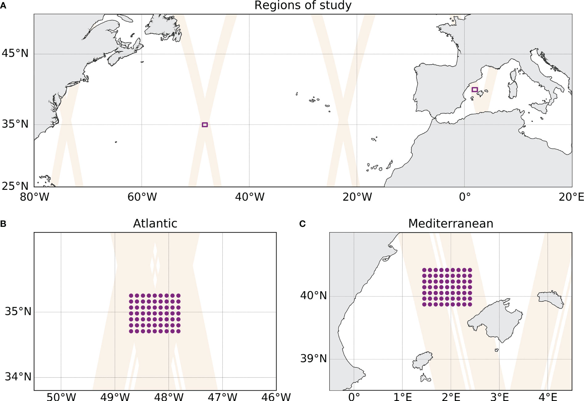
Figure 1 (A) Map with the regions of study (magenta boxes) and the swaths of SWOT during the fast-sampling phase (orange bands). (B, C) show a zoom around the regions of study. (B) SWOT crossover in the subpolar northwest Atlantic (orange bands) with the position of the reference configuration CTD casts (magenta dots). (C) Swaths of SWOT in the northwestern Mediterranean (orange bands) with the position of the reference configuration CTD casts (magenta dots). The coordinates of the swaths of SWOT were extracted from the simulated SWOT product from the MITgcm LLC4320 model (L2_LR_SSH), available on the AVISO website: http://doi.org/10.24400/527896/a01-2021.006.

2.2 Nature run models

In each region of study different nature run models are used to simulate the observations in distinct configurations and also to represent the ocean truth. Each model has different characteristics and resolutions (see description below), and they are selected for this study to evaluate the robustness of the results. The models used in each region are:

● Atlantic: CMEMS global reanalysis and eNATL60

● Mediterranean: CMEMS Mediterranean reanalysis, eNATL60 and WMOP

2.2.1 CMEMS reanalyses

The Copernicus Marine Environment Monitoring Service (CMEMS) global ocean physics reanalysis used in the Atlantic experiments has a spatial resolution of 1/12° and 50 vertical levels (Lellouche et al., 2021). The model component is the Nucleus for European Modelling of the Ocean (NEMO) platform driven at the surface by the ECMWF ERA-Interim atmospheric reanalysis. Along-track altimeter Sea Level Anomaly (SLA), satellite Sea Surface Temperature (SST), Sea Ice Concentration and in situ temperature and salinity vertical profiles are assimilated. This product includes daily and monthly mean fields of temperature, salinity, currents, sea level, mixed layer depth and ice parameters from the surface to bottom, and covers the period from 1993 onwards. For our experiments we use the daily mean fields. The model outputs are available at https://doi.org/10.48670/moi-00021.

The CMEMS Mediterranean Sea physics reanalysis used in the Mediterranean experiments has a spatial resolution of 1/24° and 141 vertical levels (Escudier et al., 2020). This product is generated by a numerical system consisting of a hydrodynamic model supplied by NEMO and a variational data assimilation scheme (OceanVAR). It assimilates in situ temperature and salinity vertical profiles and satellite along-track SLA and SST. This product includes hourly, daily and monthly mean fields of temperature, salinity, currents, sea level and mixed layer depth from the surface to bottom, and covers the period from 1987 to present. For the experiments in the Mediterranean we use the daily mean fields for consistency with the CMEMS reanalysis used in the Atlantic experiments. The Mediterranean reanalysis has been validated and assessed by Escudier et al. (2021) and used in several studies (e.g. Martínez et al., 2022; Sannino et al., 2022).

2.2.2 eNATL60

eNATL60 corresponds to a pair of twin numerical ocean simulations performed with the NEMO model over the North Atlantic and including the Gulf of Mexico, the Mediterranean Sea, and the Black Sea. The horizontal resolution is 1/60° and it has 300 vertical levels. The model configuration was defined to resolve as accurately as possible the surface signature of oceanic motions of scales down to 15 km, in accordance with the expected effective resolution of SWOT observations (Ajayi et al., 2020). This model configuration was implemented and run in two different free-run simulations (no data assimilation): one experiment including explicit tidal forcing and the other experiment without tidal forcing. In this study we use the simulation without tidal forcing and hourly outputs. Several studies have used the non-extended version of this model, called NATL60 (e.g. Amores et al., 2018; Fresnay et al., 2018; Metref et al., 2019; Ajayi et al., 2020; Metref et al., 2020; Ajayi et al., 2021; Le Guillou et al., 2021).

2.2.3 WMOP

The Western Mediterranean Operational system (WMOP) is a regional configuration of the Regional Ocean Modelling System (ROMS, Shchepetkin and McWilliams, 2005) in the western Mediterranean Sea, covering from Gibraltar strait to Corsica and Sardinia (Juza et al., 2016; Mourre et al., 2018). It is a downscaling of the Mediterranean sea physical reanalysis CMEMS-MED-MFC (Simoncelli et al., 2019) with a ~2 km horizontal resolution and 32 vertical sigma levels. Here we use a free-run hindcast simulation based on the WMOP forecasting system configuration that covers the period 2009–2015. This hindcast has been validated by Mourre et al. (2018) and Aguiar et al. (2020).

2.3 Simulated observations

Vertical profiles of temperature and salinity were simulated following the same procedure for the three platforms equipped with CTD probes: rosette CTD, underway CTD (or uCTD) and gliders. For each CTD profile, defined by its spatial coordinates and time, we extracted the corresponding data from model outputs using a four-dimensional linear interpolation in time, depth, latitude and longitude. The variables extracted were potential temperature and practical salinity. For eNATL60 a previous interpolation was needed to rotate the original model outputs in an oblique grid onto a regular grid for each time step and depth level, while the spatial resolution of 1/60° was maintained. Simulated observations are assumed perfect, i.e., no instrumental errors are included (Le Guillou et al., 2021). With this approach we ensure that the differences between reconstructed fields are not affected by simulated errors and they are only due to the configuration design and sampling duration.

2.4 Configurations

Several configurations of the in situ experiment were simulated to evaluate the best sampling strategy to reconstruct fine-scale (~20 km) ocean currents and validate SWOT measurements during the fast-sampling phase. The reference configuration is similar to the PRE-SWOT sampling strategy in both regions of study (Barceló-Llull et al., 2021). With additional configurations we study the impact of changing the separation between CTD profiles, their maximum vertical extension, the temporal variability, and also the effect of replacing rosette CTD casts for a continuous underway CTD or gliders. The parameters defining each configuration are shown in Tables 1, 2. All configurations start on a common date in summer (1 September 2009), except configuration 4, which is conducted in winter (1 January 2010). Some assumptions were made to simulate these designs based on the knowledge gained in similar field experiments (Barceló-Llull et al., 2017b; Mahadevan et al., 2020; Barceló-Llull et al., 2021):

● The experiment begins in the northwest corner of the domain. The research vessel samples the first zonal transect from west to east, moves southward to the next zonal transect and samples the second transect from east to west; repeat for the other transects.

● The research vessel navigates with a constant speed of 8 knots and stops to release the rosette CTD casts. The time needed to sample the water column down to 500 m is 30 min, and down to 1000 m is 60 min. We assume that during the CTD cast the water column properties do not change and we extract the model data corresponding to the time of the cast release.

● For the strategies including an underway CTD we assume a constant ship velocity of 8 knots.

● The configuration with gliders consists of 7 gliders, each one sampling simultaneously one zonal transect from east to west at a constant horizontal velocity of 0.25 m/s.

TABLE 1

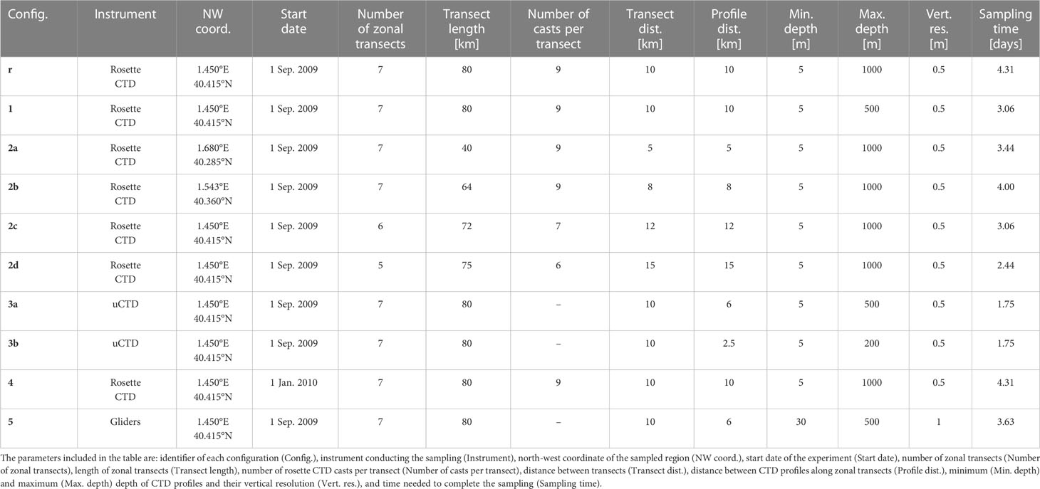
Table 1 Description of the configurations simulated in the Mediterranean study region.

TABLE 2

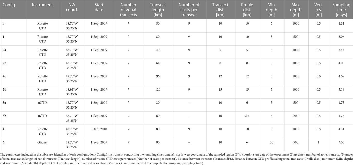
Table 2 Description of the configurations simulated in the Atlantic study region.

2.5 Spatio-temporal optimal interpolation and reconstructed fields

The optimal interpolation algorithm usually used to reconstruct in situ observations in field experiments only considers the spatial variability of the measurements and assumes quasi-synopticity at the scales resolved by the sampling (e.g., Rudnick, 1996; Pascual et al., 2004; Barceló-Llull et al., 2017b; Ruiz et al., 2019; Barceló-Llull et al., 2021). However, if the structures evolve during the sampling period, the observations are not synoptic and the reconstruction may introduce errors. For this analysis we use an advanced version of the optimal interpolation that also considers the time coordinate of each observation and from which the resulting map represents a specific date of the sampling period. This method is applied to reconstruct altimetry observations (e.g., Escudier et al., 2013) and also includes the temporal correlation scale in the correlation function of the optimal interpolation. This function is used to compute correlations between observational points to determine the weights for the data interpolation. Then, to compute the correlation between grid and observational points, we use the same correlation function assuming that the interpolation maps the observations on the central date of the sampling.

To determine the appropriate spatial and temporal correlation scales for the spatio-temporal optimal interpolation, we performed an extensive analysis (Barceló-Llull et al., 2022a). In summary, fixing the spatial correlation scales to 20 km (∼scales resolved by SWOT, Barceló-Llull et al., 2021), we tested the sensitivity of the temporal correlation scale on the reconstruction of SSH fields in the Mediterranean (from eNATL60 and WMOP) and in the Atlantic (from eNATL60) in 52 sampling periods evaluated over a year. The two extreme values studied (2 and 10 days) provided different reconstructions, but both fields were consistent with the ocean truth and led to almost identical RMSE-based scores (see metric definition in the next section). This analysis concluded that using a temporal correlation scale of 10 days, and assuming quasi-synoptic observations, was a valid option for the interpolation of observations in a sampling strategy similar to the reference design.

The simulated temperature and salinity measurements (or pseudo-observations) were interpolated onto a 3D regular grid with a horizontal resolution of 2 km and a vertical spacing of 5 m. The new grid was defined for each configuration by the longitude and latitude limits of the original CTD domain. Linear interpolation was applied on the vertical and the spatio-temporal optimal interpolation algorithm was implemented horizontally. We used spatial correlation scales of 20 km and a temporal correlation scale of 10 days. The mean fields were assumed to be planar and the uncorrelated noise for the interpolation of temperature and salinity was assumed to be 3% of the signal energy (Barceló-Llull et al., 2021).

With the reconstructed temperature and salinity 3D fields, we computed the dynamic height (DH) and the corresponding geostrophic velocity at the ocean upper layer (5 m for the configurations with CTD/uCTD and 30 m for the configuration with gliders) assuming a reference level of no motion at the maximum depth of the CTD profiles. This is the procedure that will be followed to validate SWOT measurements with real in situ observations during the fast-sampling phase (Barceló-Llull et al., 2021).

2.6 Evaluation of different sampling strategies

To evaluate the configurations simulated in each region, we compare the reconstructed variables (DH and geostrophic velocity) to the corresponding ocean truth fields (SSH and horizontal velocity) through the root-mean-square error (RMSE) and the RMSE-based score (RMSEs or score), defined as 1 – [RMSE/RMS(ocean truth)], where RMS is the root-mean-square function. A RMSEs of 1 indicates a perfect reconstruction in terms of the RMSE, while a score of 0 indicates that the RMSE is as large as the RMS of the ocean truth (Le Guillou, et al., 2021). The statistical metrics are computed over the same area for all designs to avoid sensitivity of the results to the domain size. The procedure comprises the following steps:

● Extract model fields (considered the ocean truth) in a bigger domain than the corresponding configuration. Linearly interpolate them to the date and grid of the reconstruction.

● Limit model and reconstructed fields within the domain of configuration 2a.

● Compute anomalies of DH and SSH subtracting the spatial average of each field over the new domain.

● Calculate the RMSE and RMSE-based score between reconstructed and model fields, for each configuration, model and region.

Maps of the reconstructed and ocean truth fields are shown in Figures 2–6, and the statistics are represented in Tables 3, 4. To evaluate the results we analyze the strategies simulated in each region for each model, based on the statistics computed from the DH and geostrophic velocity reconstructions. Then we discuss the results to provide general conclusions for each region.

FIGURE 2

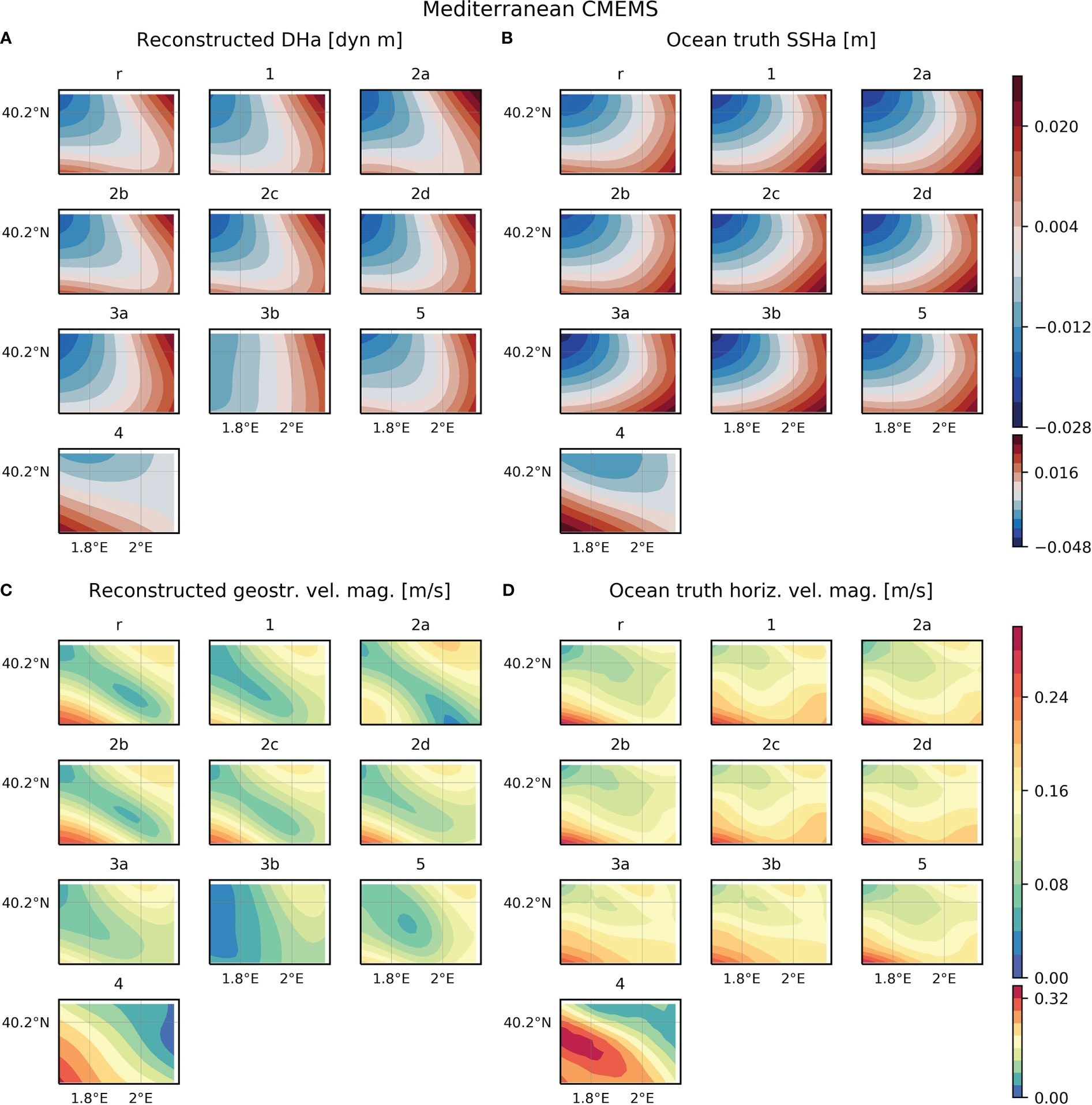
Figure 2 (A) Dynamic height anomaly (DHa) at the upper layer reconstructed from each configuration simulated from the CMEMS Mediterranean reanalysis in the Mediterranean study region. (B) Sea surface height anomaly (SSHa) from the CMEMS Mediterranean reanalysis on the same date as each reconstruction. To compute anomalies, the spatial average is subtracted to the corresponding field. (C) Geostrophic velocity magnitude at the upper layer reconstructed from each configuration simulated from the CMEMS Mediterranean reanalysis in the Mediterranean study region. (D) Horizontal velocity magnitude from the CMEMS Mediterranean reanalysis on the same date as each reconstruction. Note that to calculate statistics model fields are interpolated onto the reconstruction grid and statistics are computed only considering data within the domain of configuration 2a.

FIGURE 3

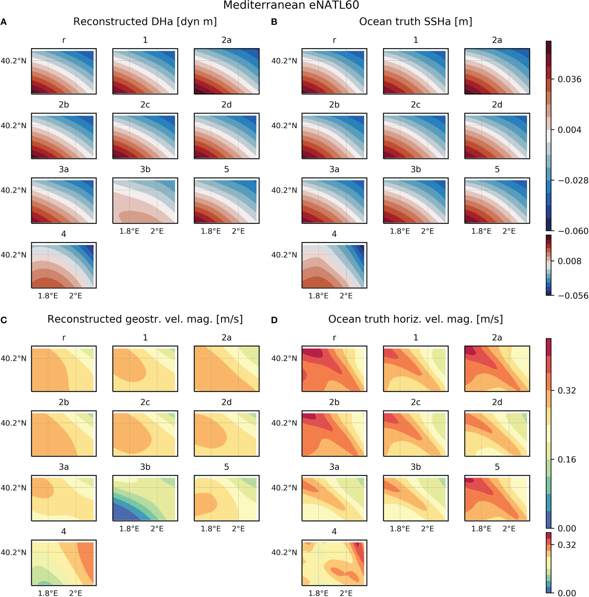
Figure 3 (A) Dynamic height anomaly (DHa) at the upper layer reconstructed from each configuration simulated from the eNATL60 model in the Mediterranean study region. (B) Sea surface height anomaly (SSHa) from eNATL60 on the same date as each reconstruction. To compute anomalies, the spatial average is subtracted to the corresponding field. (C) Geostrophic velocity magnitude at the upper layer reconstructed from each configuration simulated from eNATL60 in the Mediterranean study region. (D) Horizontal velocity magnitude from eNATL60 on the same date as each reconstruction. Note that to calculate statistics model fields are interpolated onto the reconstruction grid and statistics are computed only considering data within the domain of configuration 2a.

FIGURE 4

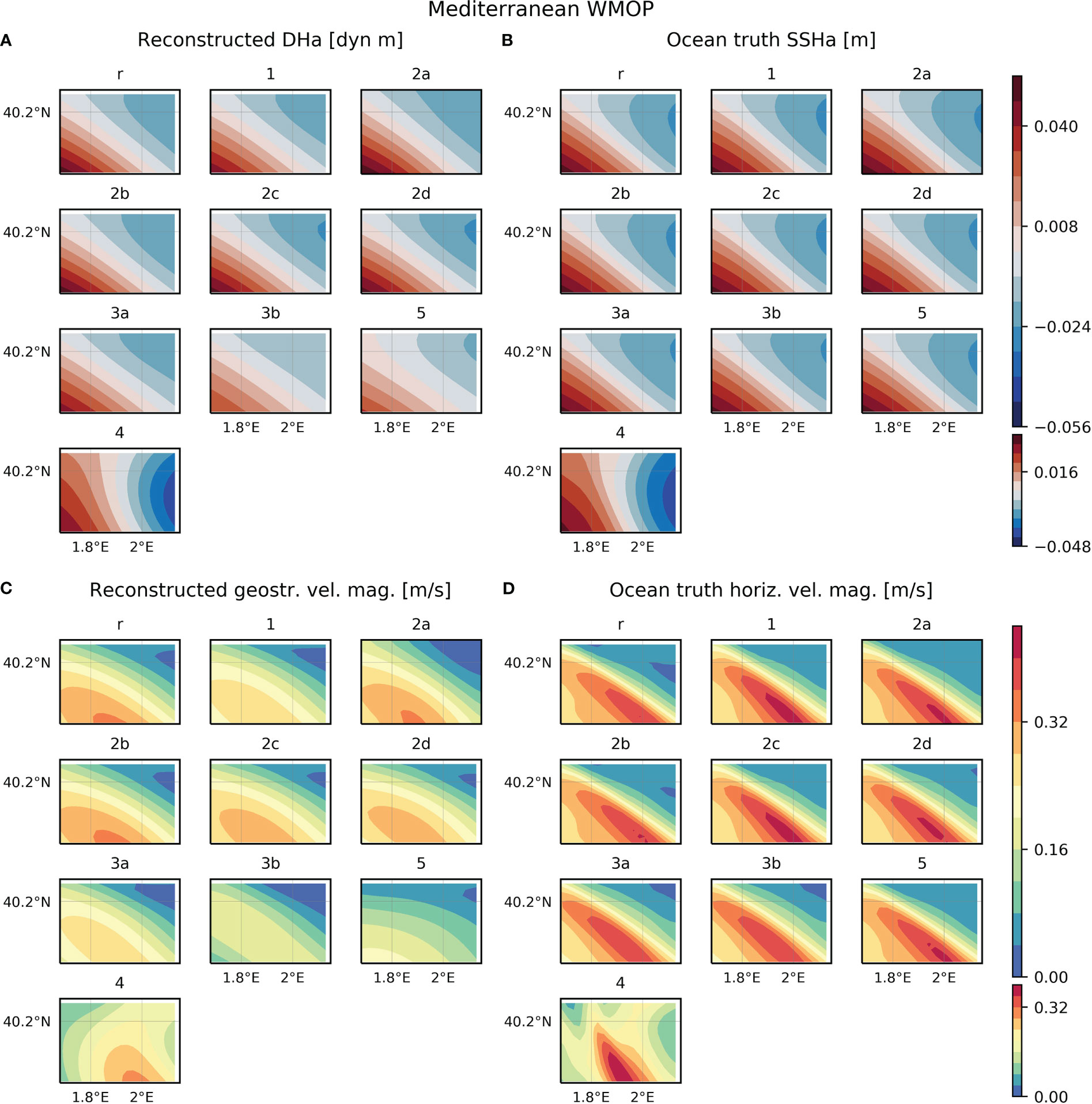
Figure 4 (A) Dynamic height anomaly (DHa) at the upper layer reconstructed from each configuration simulated from the WMOP model in the Mediterranean study region. (B) Sea surface height anomaly (SSHa) from WMOP on the same date as each reconstruction. To compute anomalies, the spatial average is subtracted to the corresponding field. (C) Geostrophic velocity magnitude at the upper layer reconstructed from each configuration simulated from WMOP in the Mediterranean study region. (D) Horizontal velocity magnitude from WMOP on the same date as each reconstruction. Note that to calculate statistics model fields are interpolated onto the reconstruction grid and statistics are computed only considering data within the domain of configuration 2a.

FIGURE 5

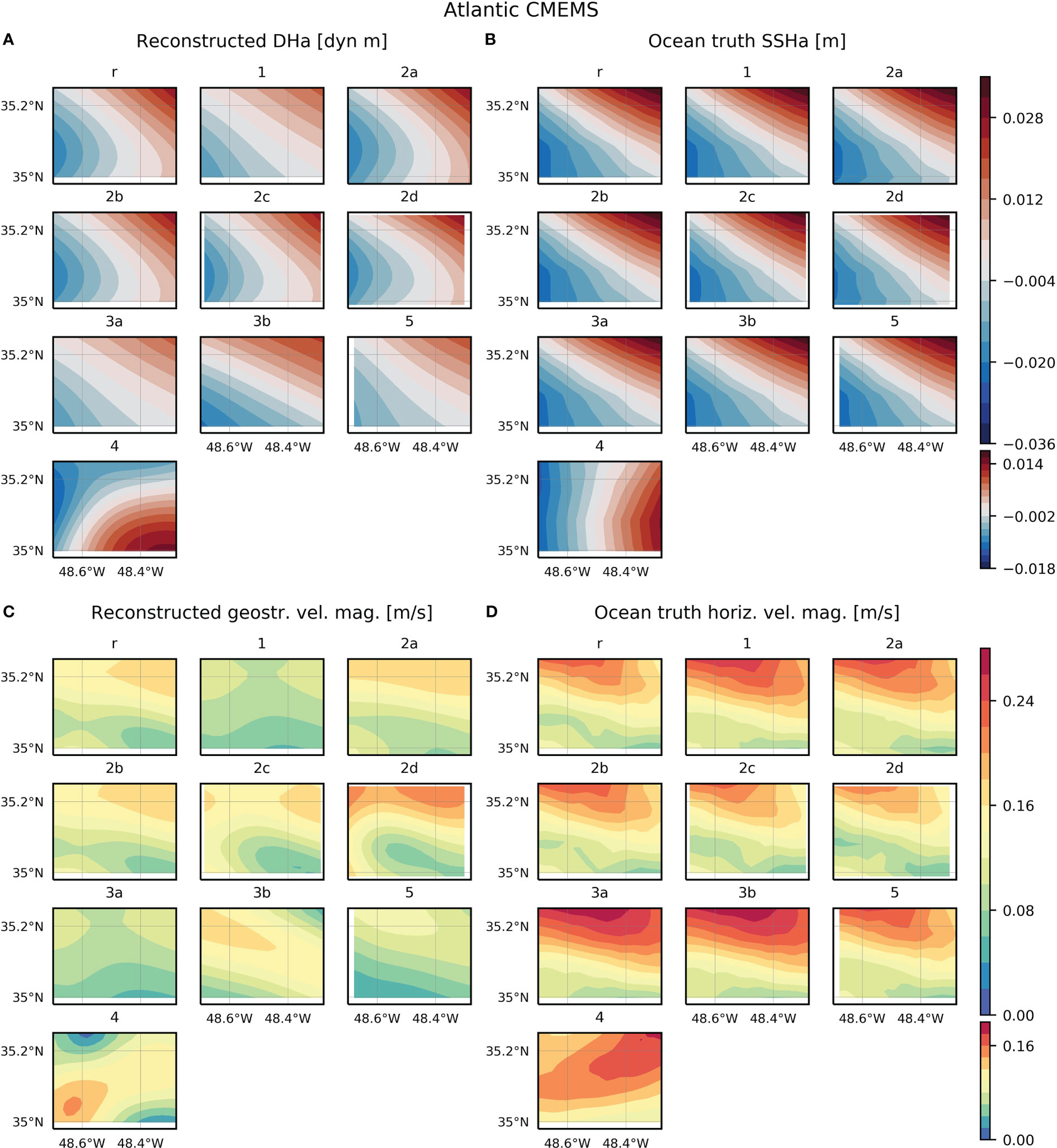
Figure 5 (A) Dynamic height anomaly (DHa) at the upper layer reconstructed from each configuration simulated from the CMEMS global reanalysis in the Atlantic study region. (B) Sea surface height anomaly (SSHa) from the CMEMS global reanalysis on the same date as each reconstruction. To compute anomalies, the spatial average is subtracted to the corresponding field. (C) Geostrophic velocity magnitude at the upper layer reconstructed from each configuration simulated from the CMEMS global reanalysis in the Atlantic study region. (D) Horizontal velocity magnitude from the CMEMS global reanalysis on the same date as each reconstruction. Note that to calculate statistics model fields are interpolated onto the reconstruction grid and statistics are computed only considering data within the domain of configuration 2a.

FIGURE 6

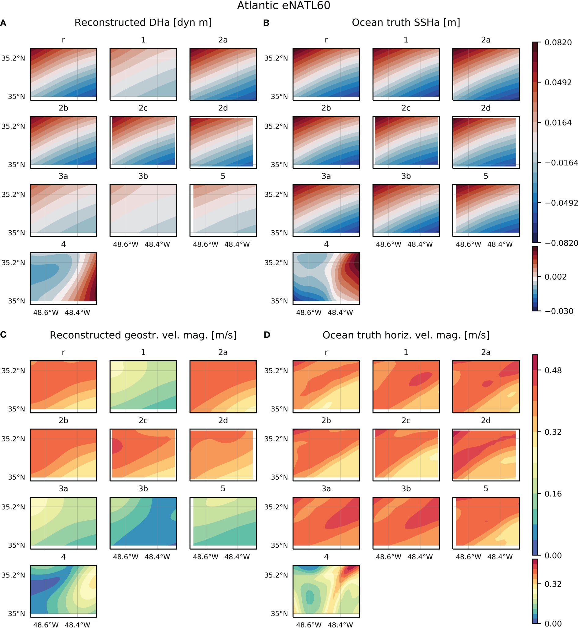
Figure 6 (A) Dynamic height anomaly (DHa) at the upper layer reconstructed from each configuration simulated from the eNATL60 model in the Atlantic study region. (B) Sea surface height anomaly (SSHa) from eNATL60 on the same date as each reconstruction. To compute anomalies, the spatial average is subtracted to the corresponding field. (C) Geostrophic velocity magnitude at the upper layer reconstructed from each configuration simulated from eNATL60 in the Atlantic study region. (D) Horizontal velocity magnitude from eNATL60 on the same date as each reconstruction. Note that to calculate statistics model fields are interpolated onto the reconstruction grid and statistics are computed only considering data within the domain of configuration 2a.

TABLE 3

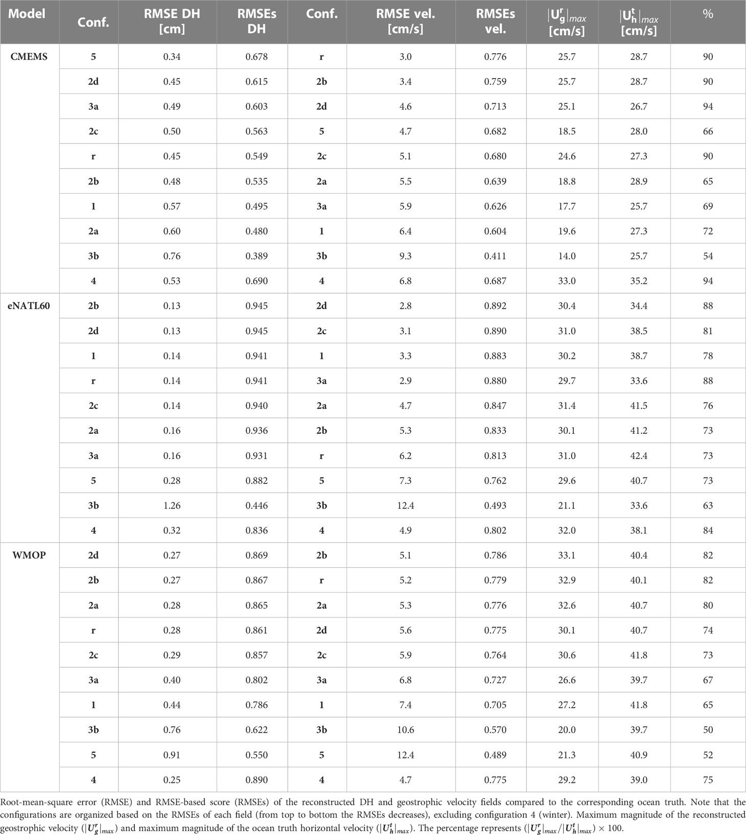
Table 3 Statistics for the configurations simulated in the Mediterranean from the three models: CMEMS Mediterranean reanalysis, eNATL60 and WMOP.

3 Results and discussion

3.1 Analysis in the Mediterranean

3.1.1 Comparison based on the DH reconstruction

The statistics computed for the configurations simulated from eNATL60 reveal that several designs have scores higher than 0.93, with a RMSE between 0.13 and 0.16 cm (Table 1). This indicates that different strategies provide reconstructions of DH similar to the ocean truth: reference, 1, 2a-d and 3a. Configuration 5, consisting of 7 gliders sampling zonal transects simultaneously down to 500 m depth and with a separation between profiles of 6 km, has a lower score than the other designs (0.88) and a RMSE of 0.28 cm.

For the strategies simulated from WMOP, the configurations that consider CTD casts down to 1000 m (reference, 2a-d) have similar scores of ~0.86 and a RMSE between 0.27-0.29 cm. The sampling of the water column down to 500 m with rosette CTD and underway CTD (configurations 1 and 3a) provides reconstructions with lower scores (~0.80) and higher RMSE (0.44 and 0.40 cm, respectively). The configuration with gliders has the lowest RMSEs (0.55) and a RMSE of 0.91 cm.

In contrast to the results obtained for the other models, the strategy simulated from the CMEMS reanalysis with the highest score is the configuration with gliders (RMSEs = 0.68, RMSE = 0.34 cm). The reference design and configurations 1, 2a-d and 3a have scores from 0.48 to 0.62 and a RMSE of 0.45-0.60 cm. In this case, the distinction in the strategies observing the upper 500 m vs. 1000 m is not detected.

For the three models analyzed, configuration 3b provides reconstructions with low scores compared to the other designs (except for WMOP, in which configuration 5 has the lowest score). This strategy consists of an underway CTD sampling one profile every 2.5 km and with a vertical extension of 200 m. Maps of the DH anomaly show that for this configuration the extreme values are lower than for the other strategies and ocean truth (Figures 2A, B, 3A, B, 4A, B).

Regarding seasonality, configuration 4, consisting of the same design as the reference strategy but in winter instead of in summer, provides reconstructions with high scores for the three models evaluated (Table 3). These values are higher than the scores obtained in summer for WMOP and CMEMS, and lower for eNATL60. The RMSE increases in winter for eNATL60 and CMEMS, while decreases for WMOP.

3.1.2 Comparison based on the geostrophic velocity reconstruction

With eNATL60 several strategies have scores higher than 0.81: reference, 1, 2a-d and 3a (Table 3). In all cases, the reconstructed geostrophic velocity has a lower magnitude than the ocean truth (Figures 3C, D) and its maximum value represents between ~70-90% of the ocean truth maximum speed (Table 3). The differences in this percentage are related to the maximum magnitude of the ocean truth, which differ between configurations, while the reconstructed maximum speed is maintained at about 30 cm/s (Table 3). On the other hand, the strategy with gliders has a RMSEs of 0.76, a RMSE of 7.3 cm/s and a representation of the ocean truth maximum speed of 73%. Configuration 3b provides the reconstruction with the lowest score (0.49) and the highest RMSE (12.4 cm/s), and represents 63% of the ocean truth maximum speed. Concerning seasonality, the reconstructed geostrophic velocity for configuration 4 has a RMSEs similar to the value obtained in summer. Note that in winter the reconstructed field is not able to represent the small scales observed in the ocean truth (Figures 3C,D). This is expected due to the sampling resolution (10 km) and the spatial correlation scales (20 km) used in the optimal interpolation.

Regarding the strategies simulated from WMOP, the highest scores are obtained for those designs consisting of CTD profiles down to 1000 m depth (Table 3). The strategies with a separation of 5 km (2a), 8 km (2b) and 10 km (reference) represent the geostrophic velocity with a slightly higher magnitude than those with a horizontal spacing of 12 km (2c) and 15 km (2d). On the other hand, configurations 1 and 3a capture a lower magnitude than the previous sampling strategies. The reconstructed field from configuration 1 has a RMSE of 7.4 cm/s and the maximum speed represents 65% of the ocean truth, while with strategy 3a the RMSE is 6.8 cm/s and the percentage is 67%. Strategy 3b captures 50% of the ocean truth maximum speed. The configuration with the lowest score is the sampling strategy with gliders. In this case, the reconstructed maximum magnitude represents 52% of the ocean truth maximum speed. Regarding seasonality, configuration 4 provides a reconstruction with similar statistics to the values obtained in summer.

The configuration simulated from the CMEMS reanalysis with the highest score is the reference design (0.78, RMSE = 3.0 cm/s), followed by configurations 2b, 2d, 5, 2c, 2a, 3a and 1 (Table 3). The reference design and strategies 2b-d reconstruct a similar pattern of geostrophic velocity magnitude with a maximum value that represents ~90% of the ocean truth maximum magnitude (Figures 2C, D). Configuration 2a, with a CTD vertical extension of 1000 m and a horizontal separation between profiles of 5 km, reconstructs a maximum magnitude that is 65% of the ocean truth. Note that the highest speed detected in the reconstructed fields for the reference configuration and strategies 2b-d is located at the southwest corner of the domain. These designs may have been able to capture this feature because the sampling region is bigger than in strategy 2a. The strategy with gliders provides a reconstruction with a score of 0.68 (RMSE = 4.7 cm/s) that captures 66% of the ocean truth maximum speed. The other two strategies with profiles down to 500 m depth (3a and 1) reconstruct fields with lower scores and higher RMSE (5.9 and 6.4 cm/s, respectively) that capture ~70% of the ocean truth maximum horizontal velocity magnitude. The reconstruction with the lowest score is for configuration 3b (0.41, RMSE = 9.3 cm/s); the magnitude captured by this strategy represents 54% of the ocean truth maximum speed. Regarding seasonality, the reconstructed field for configuration 4 is smoother than the ocean truth, but the overall pattern is consistent with a slight underestimation of the magnitude (Figure 2D). The reconstructed maximum speed represents ~94% of the ocean truth maximum value.

3.1.3 Discussion

3.1.3.1 Best sampling strategies to reconstruct fine-scale currents

To evaluate the best sampling strategies in the Mediterranean, we focus on the results obtained for each model considering the two variables analyzed: DH and geostrophic velocity.

With eNATL60 seven configurations (reference, 1, 2a-d, 3a) have high scores for the reconstruction of the DH (RMSEs>0.93) and geostrophic velocity magnitude (RMSEs>0.81). In all cases, the reconstructed velocity has an inferior magnitude than the ocean truth horizontal velocity. With these strategies, the maximum speed of the reconstructed currents represents between ~70-90% of the ocean truth maximum velocity. The differences detected between configurations are related to the maximum speed of the ocean truth, which is distinct for each configuration. Because of this, the results from eNATL60 suggest that distinct strategies provide reconstructions similar to the ocean truth and, hence, they are valid designs.

From WMOP, a difference is detected in the reconstruction of both fields between those strategies sampling 1000 m depth and the designs that only observe the upper 500 m. The first set of configurations (reference, 2a-d) have the leading scores, and their reconstructed currents represent between ~70-80% of the ocean truth maximum speed. In the second set of strategies, configurations 3a and 1 capture ~65% of the ocean truth maximum speed with a RMSE of ~7 cm/s, while configuration 5 represents a ~50% and has a RMSE of ~12 cm/s.

For the strategies simulated from the CMEMS Mediterranean reanalysis, the DH reconstruction with the leading score is for the design with gliders, in contrast to the results obtained for the other models. Otherwise, the best score for the geostrophic velocity reconstruction is for the reference configuration, a result that is consistent with the other models. In this case, the reference design and configurations 2b-d capture ~90% of the ocean truth maximum speed, while configuration 2a represents a smaller percentage due to different sizes of the sampling domain. Regarding the strategies measuring the upper 500 m depth (configurations 5, 3a, 1), they capture ~70% of the ocean truth maximum magnitude.

Considering the results from three models with distinct temporal and spatial resolutions, the conclusion from this analysis is that several sampling strategies are valid designs to reconstruct fine-scale ocean currents in the studied scenario. The designs consisting of a rosette CTD sampling the water column down to 1000 m depth and assuming distinct horizontal separation between profiles (5-15 km) provide the reconstructions more similar to the ocean truth. However, the horizontal separation between profiles is key because it determines (i) the sampling time (larger separation implies faster sampling of the same domain) and/or (ii) the domain extension that can be measured in a fixed period of time.

The sampled domains of the configurations simulated in the Mediterranean were located within a swath of SWOT, and their extension was limited by the local bathymetry. For the reference design and configurations 1, 2a and 2b the total number of casts was fixed to 63 (7 zonal transects with 9 casts each, assuming distinct distances between them), while for configurations 2c and 2d this number was reduced in order to limit the domain in a bathymetry deeper than 1000 m depth (Table 1). This implies that the sampling time increases when enlarging the horizontal separation between casts (and, hence, the size of the sampled domain) for configurations 2a (5 km), 2b (8 km) and reference (10 km) (Table 1). On the other hand, the reference design and configurations 2c (12 km) and 2d (15 km) have a different number of casts while the sampled domain has a similar size [see figures 12, 15, 17, 19 and 21 in Barceló-Llull et al. (2022a)]. Because of this, the sampling time is shortened between the reference design and configurations 2c and 2d (Table 1).

Considering the specific characteristics of these strategies, with a cast separation of 5 and 8 km the domain sampled is smaller than for the reference design in order to maintain the number of casts to 63 (Barceló-Llull et al., 2021), while with a separation of 12 and 15 km the same domain as for the reference design is sampled faster, decreasing the spatial resolution but obtaining valid reconstructions for the period evaluated. A good compromise considering the advantages of each strategy is the reference configuration, consisting of CTD casts separated by 10 km and down to 1000 m depth. To sample the same domain in a shorter period of time, an alternative is to release the CTD casts down to 500 m depth (configuration 1). With this strategy and based on the results from WMOP (CMEMS), the reconstructed geostrophic velocity has a maximum speed that represents 65% (72%) of the ocean truth maximum velocity, while for the reference configuration this percentage is 82% (90%). Another option is to replace the rosette CTD casts for an underway CTD with a horizontal spacing between profiles of 6 km and a vertical extension of 500 m (configuration 3a). This strategy has the advantage of sampling the same domain in 1.8 days in comparison to 4.3 days for the reference configuration and 3.1 days for configuration 1. In this case, based on the results from WMOP (CMEMS), the geostrophic velocity maximum magnitude represents 67% (69%) of the ocean truth.

3.1.3.2 Sampling strategy not appropriate for our objective

A result that is clear from the analysis in the Mediterranean is that the strategy in which rosette CTD casts are replaced by an underway CTD sampling one profile every 2.5 km and with a vertical extension of 200 m is the configuration with the lowest scores for eNATL60 and CMEMS, and the second with the lowest scores for WMOP for the two variables analyzed. Maps of reconstructed geostrophic velocity show that for this configuration the reconstructed field has lower magnitude than for the ocean truth and the other reconstructions, with the exception of configuration 5 for WMOP. This suggests that profiles deeper than 200 m depth are needed to reconstruct the DH and geostrophic velocities at the ocean upper layer, while the decrease of the horizontal separation between profiles does not introduce improvements with respect to the other configurations.

3.1.3.3 Impact of season

Configuration 4, which consists of the same design as the reference but in winter instead of in summer, has high scores for the DH and geostrophic velocity reconstructions with the three models. Note that different dynamics characterize the region of study in each season. In summer the upper layer is stratified due to solar warming, while in winter there is a mixed layer that decreases the vertical gradient of density. As a consequence, the first Rossby radius of deformation is reduced in winter and the structures are smaller (Chelton et al., 1998; Barceló-Llull et al., 2019). This is supported by the study of the spatial correlation scales conducted by Barceló-Llull et al. (2022a) through the empirical correlation calculated from pseudo-observations of temperature and salinity, and also from the original model data, for each model and region (Mediterranean and Atlantic). With both approaches they found that in winter the scales are ~5 km smaller than in summer in both regions. The sampling resolution of 10 km and the spatial correlation scales of 20 km applied to the optimal interpolation prevent the representation of spatial scales smaller than ~20 km. This results in smoother reconstructed fields of geostrophic velocity in comparison to the ocean truth in winter. Besides this, with eNATL60 the RMSEs in winter is still elevated (0.80) and comparable to the score obtained in summer (0.81). For WMOP the outcome is similar and the RMSEs in winter is 0.77 in front of 0.78 in summer. With the CMEMS reanalysis the RMSEs is 0.69 vs. 0.78 in summer. In conclusion, even with distinct dynamics, the reference configuration is a sampling strategy that provides reconstructions similar to the ocean truth in both seasons for the three models evaluated.

3.2 Analysis in the Atlantic

3.2.1 Comparison based on the DH reconstruction

For the sampling strategies simulated from the CMEMS reanalysis, two distinct designs provide the highest scores for the DH reconstruction (Table 4): configuration 3b, with a horizontal separation between profiles of 2.5 km, a vertical extension of 200 m and the lowest sampling time (1.8 days), and configuration 2d, with a spatial resolution of 15 km, a vertical extension of 1000 m and with the highest sampling time (5.2 days). The contrasting characteristics of both strategies and the smooth reconstructed fields of DH (Figures 5A, B) difficult the interpretation of this result and make necessary the analysis of the reconstructed geostrophic velocity magnitude. A result that is clear from the remaining configurations is that the strategies consisting of CTD profiles down to 1000 m depth (reference, 2a-c) have similar scores of ~0.6 (RMSE = ~0.6 cm), while the strategies that sample the water column down to 500 m depth (5, 3a and 1) have lower scores (~0.5, RMSE = ~0.7 cm). Concerning seasonality, configuration 4 has a RMSEs of 0.27, much lower than the reference design, with a RMSE in both scenarios of 0.55 cm.

TABLE 4

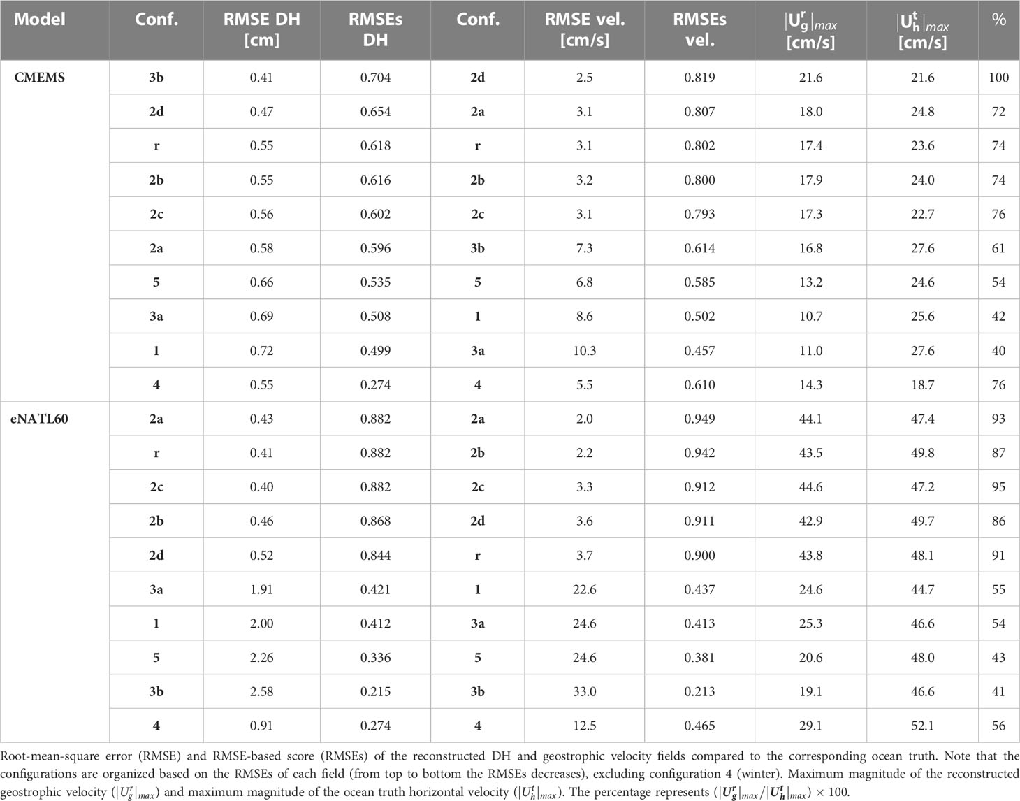
Table 4 Statistics for the configurations simulated in the Atlantic from two different models: CMEMS global reanalysis and eNATL60.

With eNATL60 the difference observed previously between the strategies sampling the upper 1000 m depth versus only the upper 500 m is more evident (Figures 6A, B and Table 4). The first set of designs (reference, 2a-d) have scores higher than 0.84 (RMSE = 0.40-0.52 cm), while the second set (3a, 1, 5) have scores below 0.42 (RMSE = 1.90-2.30 cm). Configuration 3b, only considering profiles down to 200 m depth, has the lowest score (0.22, RMSE = 2.58 cm). The dissimilarities between reconstructions can be clearly observed in the DH maps (Figures 6A, B): for the reference design and configurations 2a-d the reconstructed DH has a magnitude and pattern similar to the ocean truth, while for the other strategies the magnitude is underestimated. Configuration 4 reconstructs the DH with a low RMSEs of 0.27 (RMSE = 0.91 cm), similar to the result obtained for the CMEMS reanalysis.

3.2.2 Comparison based on the geostrophic velocity reconstruction

The statistics computed for the geostrophic velocity support the results derived from the analysis of the DH. The configurations consisting of CTD profiles down to 1000 m depth (reference, 2a-d) have the highest scores for both models (Table 4). Maps of the geostrophic velocity magnitude for the strategies simulated from CMEMS show that the reference design and configurations 2a-d have higher values than for the other configurations (Figure 5C). The strategy 2d has a maximum magnitude that represents 100% of the ocean truth maximum speed, while the reference design and configurations 2a-c capture 72-76% of this signal (Table 4). For these configurations the RMSEs is higher than 0.8 and the RMSE is about 3 cm/s. The designs with profiles down to 500 m depth have a comparable magnitude between them and this is 40-54% smaller than the ocean truth maximum speed. The pattern of the geostrophic velocity magnitude for the configuration with gliders is closer to the ocean truth than the other strategies sampling the upper 500 m depth (Figures 5C, D), this results in a higher score (0.585, RMSE = 6.8 cm/s). Strikingly, configuration 3b, with profiles down to 200 m depth, reconstructs a geostrophic velocity field with a higher magnitude than the configurations with profiles down to 500 m depth (RMSEs = 0.614, RMSE = 7.3 cm/s).

For the configurations simulated from eNATL60, the strategies with profiles down to 1000 m have a geostrophic velocity magnitude and pattern closer to the ocean truth than the designs that only sample the upper 500 m (Figures 6C, D); this is translated in scores higher than 0.9 and in a RMSE between 2.0-3.7 cm/s (Table 4). The maximum geostrophic velocity magnitude for these strategies represents ~90% of the ocean truth speed. When only sampling the upper 500 m depth the RMSEs is reduced to ~0.4 and the RMSE increases to 23-25 cm/s. In this case, the maximum speed of the reconstructed field represents between 43% and 55% of the ocean truth maximum magnitude. For configuration 3b this underestimation is increased to 41%, with a RMSE of 33 cm/s and a RMSEs of 0.213.

Regarding seasonality, for both models configuration 4 has lower RMSEs than the reference design. With eNATL60 the reconstructed field is smoother than the ocean truth, but the overall pattern shows some similarity (Figures 6C, D). For CMEMS, the reconstructed and ocean truth fields have large differences (Figures 5C, D).

3.2.3 Discussion

3.2.3.1 Best sampling strategies to reconstruct fine-scale currents

The main conclusion derived from the analysis in the Atlantic is that sampling strategies consisting of CTD profiles down to 1000 m depth (reference, 2a-d) provide reconstructions with higher scores than the designs that sample the water column down to 500 m depth (1, 3a, 5). This is observed in the configurations simulated from both models and for the two variables analyzed (DH and geostrophic velocity). The RMSE of the geostrophic velocity magnitude for the first set of configurations is about 3 cm/s, while for the second set is between 7-10 cm/s for the CMEMS reanalysis and 23-25 cm/s for eNATL60. The maximum magnitude represents between 70% and 100% of the ocean truth maximum speed for the deeper profiles (for eNATL60 this percentage converges to 86-95%), and 40-55% for the shallower profiles. In consequence, in the Atlantic study region the sampling of the water column down to 1000 m is key for the reconstruction of the DH and geostrophic velocity magnitude at the upper layer. This result is supported by simulating the same set of configurations with two models with distinct spatial and temporal resolutions and, hence, resolving different dynamics. In conclusion, sampling strategies consisting of CTD profiles down to 1000 m depth and with horizontal separations of 5, 8, 10, 12 and 15 km are good options to reconstruct fine-scale currents (~20 km) at the ocean upper layer in the region of study in the period analyzed. The differences in the horizontal spacing of these strategies imply that distinct sizes of the domain can be sampled for a fixed sampling period. The reference configuration, which considers a distance between casts of 10 km, is a good compromise between horizontal resolution, spatial coverage and sampling duration.

3.2.3.2 Sampling strategy not appropriate for our objective

From eNATL60, configuration 3b, in which rosette CTD casts are replaced by an underway CTD sampling one profile every 2.5 km and with a vertical extension of 200 m, has the lowest scores for both variables. The reconstructed geostrophic velocity captures 41% of the ocean truth maximum speed and has a RMSE of 33 cm/s. This result is not consistent with the outcome from the CMEMS reanalysis. However, the eNATL60 spatial and temporal resolutions are more suited for the simulation of this configuration and, hence, we disregard this design as a good option for our purpose.

3.2.3.3 Impact of season

The analysis of seasonality suggests that the reference configuration, which provides good reconstructions in summer, does not capture the structures present in the region of study in winter. One explanation may be that in winter the structures evolve faster than in summer and the lack of synopticity in the pseudo-observations introduces significant errors in the reconstruction.

4 Conclusions

We have analyzed different sampling strategies aimed to reconstruct fine-scale ocean currents (~20 km), such as those that will be conducted to validate SWOT satellite observations. From this evaluation, we provide recommendations for the design of in situ experiments that share the same objective. However, note that the analysis focuses on two domains at specific periods, one in summer and the other in winter. Consequently, we do not analyze the whole range of situations that could characterize the study regions. To overcome this issue, we use different models to simulate the same set of configurations, finding consistent results.

In the Mediterranean study region, distinct strategies provide reconstructions similar to the ocean truth and, hence, they are valid configurations. A good compromise considering the advantages of each sampling strategy is the reference configuration, consisting of CTD casts separated by 10 km and down to 1000 m, sampling the domain in 4.3 days. A faster alternative is to release the rosette CTD casts down to 500 m depth (3.1 days). An even faster option consists of changing rosette CTD casts for an underway CTD with a horizontal spacing between profiles of 6 km and a vertical extension of 500 m (1.8 days). In both cases, the geostrophic velocity maximum magnitude represents about 65% of the ocean truth maximum speed for the simulation with WMOP. A sampling strategy not appropriate for our objective is the configuration consisting of an underway CTD sampling one profile every 2.5 km and down to 200 m. Regarding seasonality, the reference configuration is a design that provides reconstructions similar to the ocean truth in summer and in winter.

In the Atlantic study region, strategies consisting of CTD profiles down to 1000 m depth provide reconstructions with higher scores than the strategies that only sample the water column down to 500 m depth. The geostrophic velocities reconstructed from the strategies that sample the upper 1000 m depth have a magnitude similar to the ocean truth, while the strategies that only sample the upper 500 m depth reconstruct a maximum magnitude ~50% smaller than the ocean truth. Different horizontal spacings between CTD profiles provide fine-scale current reconstructions with high scores. The reference configuration, which considers a distance between casts of 10 km, is a good compromise between horizontal resolution, spatial coverage and sampling duration. The configuration consisting of an underway CTD sampling one profile every 2.5 km and down to 200 m reconstructs the geostrophic velocity field with the highest RMSE (33 cm/s) while its maximum magnitude represents 41% of the ocean truth maximum speed. The analysis of seasonality suggests that the reference configuration, which provides good reconstructions in summer, does not capture the structures present in the region of study in winter.

The higher RMSE of the reconstructed geostrophic velocity detected in the Atlantic for strategies that only sample the upper 500 m depth compared to the same designs in the Mediterranean may be related to the depth of the thermocline and halocline. While in the Mediterranean the maximum stratification is concentrated in the upper ~500 m depth, in the Atlantic it expands over the 1000-m-depth sampled water column (Figure 7). This suggests that the thermocline and halocline need to be measured to reconstruct the geostrophic flow at the upper layer. In consequence, a configuration that only observes the upper 200 m depth provides reconstructions with high errors in both regions. From the OSSEs conducted in this analysis, we find that in the Mediterranean (Atlantic) the sampling of the upper 500 m depth can capture 70% (~40-50%) of the ocean truth maximum horizontal velocity magnitude, while with profiles down to 1000 m this percentage is ~80-90% (~90%). Note that to reconstruct the simulated observations a reference level of no motion has been set at the maximum CTD depth. An alternative to this approach may be to use an observed horizontal velocity field at the reference level, such as the horizontal flow measured by an ADCP, taking under consideration the separation of geostrophic and ageostrophic motions and the observational errors (Barceló-Llull et al., 2017a; Tzortzis et al., 2021).

FIGURE 7

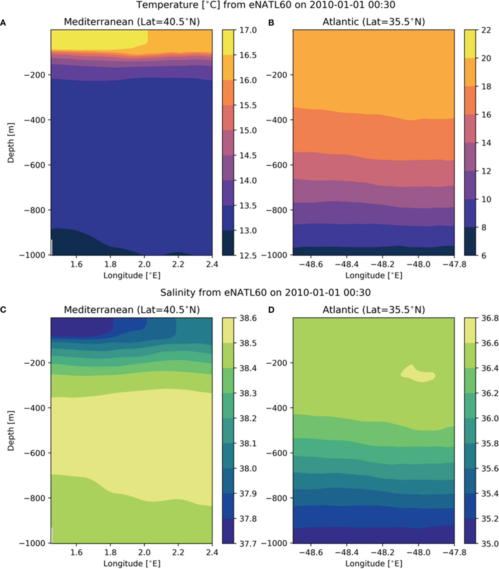
Figure 7 Zonal sections of (A, B) temperature and (C, D) salinity in the two regions of study from eNATL60 (1 January 2010, 00:30h).

The OSSEs analyzed in this study consider different designs of CTD observations to reconstruct geostrophic currents at the ocean upper layer. In real experiments, the observational strategy may also include other instruments such as an ADCP and drifters. By following a multi-platform approach, independent in situ observations will contribute to the validation of SWOT. One issue to be considered is that observations collected from different instruments have distinct sources of errors. For instance, in situ measurements can have instrumental errors, errors due to the lack of synopticity, errors associated with the data processing or due to the presence of internal waves and internal motions (d’Ovidio et al., 2019; Morrow et al., 2019). During the PRE-SWOT experiment in 2018, in preparation for the SWOT fast-sampling phase, Barceló-Llull et al. (2021) collected in situ measurements from different platforms: rosette CTD, ADCP and drifters. With this data set they could compare the geostrophic velocity derived from CTD observations with ADCP measurements of horizontal currents and drifter trajectories, finding consistency between them and a dominance of the geostrophic component of the flow. This study emphasized the benefit of following a multi-platform approach to validate SWOT in order to reduce the limitations that could arise if using observations from a single platform.

During the SWOT fast-sampling phase, two multi-platform experiments will be conducted in the western Mediterranean Sea in the framework of the FaSt-SWOT project. To design the sampling strategy of the FaSt-SWOT experiments we will follow the recommendations extracted from this study. In addition, we will explore other methods of validation based on station-keeping gliders, i.e., gliders working as moorings (called virtual moorings) following the recommendations by Wang et al. (2018). The codes developed in this study are available on GitHub and they can be used to plan other in situ experiments in different regions of the global ocean (Barceló-Llull, 2023).

Data availability statement

The dataset and codes generated in this study are available at Zenodo: Barceló-Llull et al., 2022b (https://doi.org/10.5281/zenodo.6798018); Barceló-Llull, 2023 (https://doi.org/10.5281/zenodo.7543697).

Author contributions

AP obtained the funding to develop this research. BB-L and AP designed the methodology and evaluated the results. BB-L prepared the codes for the analyses and figures, and led the writing of the manuscript.

Funding

This study was developed in the framework of the EuroSea project, funded by the European Union’s Horizon 2020 research and innovation programme under grant agreement No 862626.

Acknowledgments

We express our gratitude to the EuroSea WP2 team for supporting this research and for the fruitful discussions. We are grateful to Francesco d’Ovidio for his helpful comments concerning the interpretation of the results. We thank the interest, support and engagement of the main stakeholders of this research: the SWOT Science Team, the SWOT Adopt-A-Crossover Consortium and the FaSt-SWOT project (funded by the Spanish Research Agency and the European Regional Development Fund (AEI/FEDER, UE) under Grant Agreement (PID2021-122417NB-I00)). The present research was carried out within the framework of the activities of the Spanish Government through the "María de Maeztu Centre of Excellence" accreditation to IMEDEA (CSIC-UIB) (CEX2021-001198). This manuscript is an expanded version of a section of the report released at https://eurosea.eu referenced as Barceló-Llull et al. (2022a).

Conflict of interest

The authors declare that the research was conducted in the absence of any commercial or financial relationships that could be construed as a potential conflict of interest.

Publisher’s note

All claims expressed in this article are solely those of the authors and do not necessarily represent those of their affiliated organizations, or those of the publisher, the editors and the reviewers. Any product that may be evaluated in this article, or claim that may be made by its manufacturer, is not guaranteed or endorsed by the publisher.

References

Aguiar E., Mourre B., Juza M., Reyes E., Hernández-Lasheras J., Cutolo E., et al. (2020). Multi-platform model assessment in the western mediterranean sea: impact of downscaling on the surface circulation and mesoscale activity. Ocean. Dynamics. 70, 273–288. doi: 10.1007/s10236-019-01317-8

CrossRef Full Text | Google Scholar

Aguiar E., Mourre B., Alvera-Azcárate A., Pascual A., Mason E., Tintoré J. (2022). Strong long-lived anticyclonic mesoscale eddies in the Balearic Sea: Formation, intensification, and thermal impact. J. Geophys. Res.: Oceans 127, e2021JC017589. doi: 10.1029/2021JC017589

CrossRef Full Text | Google Scholar

Ajayi A., Le Sommer J., Chassignet E., Molines J.-M., Xu X., Albert A., et al. (2020). Spatial and temporal variability of the north Atlantic eddy field from two kilometric-resolution ocean models. J. Geophys. Res.: Oceans. 125, e2019JC015827. doi: 10.1029/2019JC015827

CrossRef Full Text | Google Scholar

Ajayi A., Le Sommer J., Chassignet E. P., Molines J.-M., Xu X., Albert A., et al. (2021). Diagnosing cross-scale kinetic energy exchanges from two submesoscale permitting ocean models. J. Adv. Modeling. Earth Syst. 13, e2019MS001923. doi: 10.1029/2019MS001923

CrossRef Full Text | Google Scholar

Amores A., Jordà G., Arsouze T., Le Sommer J. (2018). Up to what extent can we characterize ocean eddies using present-day gridded altimetric products? J. Geophys. Res.: Oceans. 123, 7220–7236. doi: 10.1029/2018JC014140

CrossRef Full Text | Google Scholar

Amores A., Monserrat S., Marcos M. (2013). Vertical structure and temporal evolution of an anticyclonic eddy in the balearic sea (western mediterranean). J. Geophys. Res.: Oceans. 118, 2097–2106. doi: 10.1002/jgrc.20150

CrossRef Full Text | Google Scholar

Ballarotta M., Ubelmann C., Pujol M.-I., Taburet G., Fournier F., Legeais J.-F., et al. (2019). On the resolutions of ocean altimetry maps. Ocean. Sci. 15, 1091–1109. doi: 10.5194/os-15-1091-2019

CrossRef Full Text | Google Scholar

Barceló-Llull B. (2023). Codes generated to evaluate in situ sampling strategies to reconstruct fine-scale ocean currents in the context of SWOT satellite mission (H2020 EuroSea project). Zenodo. doi: 10.5281/zenodo.7543697

CrossRef Full Text | Google Scholar

Barceló-Llull B., Pallàs-Sanz E., Sangrà P., Martínez-Marrero A., Estrada-Allis S. N., Arístegui J. (2017a). Ageostrophic secondary circulation in a subtropical intrathermocline eddy. J. Phys. Oceanogr. 47, 1107–1123. doi: 10.1175/JPO-D-16-0235.1

CrossRef Full Text | Google Scholar

Barceló-Llull B., Pascual A., Albert A., Beauchamp M., Fablet R., Guinehut S., et al. (2022a). Analysis of the OSSEs with multi-platform in situ data and impact on fine-scale structures. Tech. rep., H2020 EuroSea project. doi: 10.3289/eurosea_d2.3

CrossRef Full Text | Google Scholar

Barceló-Llull B., Pascual A., Albert A., Hernández-Lasheras J., Leroux S., Mourre B. (2022b). Dataset generated to evaluate in situ sampling strategies to reconstruct fine-scale ocean currents in the context of SWOT satellite mission (H2020 EuroSea project). Zenodo. doi: 10.5281/zenodo.6798018

CrossRef Full Text | Google Scholar

Barceló-Llull B., Pascual A., Ruiz S., Escudier R., Torner M., Tintoré J. (2019). Temporal and spatial hydrodynamic variability in the mallorca channel (western mediterranean sea) from 8 years of underwater glider data. J. Geophys. Res.: Oceans. 124, 2769–2786. doi: 10.1029/2018JC014636

CrossRef Full Text | Google Scholar

Barceló-Llull B., Pascual A., Sánchez-Román A., Cutolo E., d’Ovidio F., Fifani G., et al. (2021). Fine-scale ocean currents derived from in situ observations in anticipation of the upcoming SWOT altimetric mission. Front. Mar. Sci. 8. doi: 10.3389/fmars.2021.679844

CrossRef Full Text | Google Scholar

Barceló-Llull B., Sangrà P., Pallàs-Sanz E., Barton E. D., Estrada-Allis S. N., Martínez-Marrero A., et al. (2017b). Anatomy of a subtropical intrathermocline eddy. Deep. Sea. Res. Part I. 124, 126–139. doi: 10.1016/j.dsr.2017.03.012

CrossRef Full Text | Google Scholar

Bishop S. P., Small R. J., Bryan F. O. (2020). The global sink of available potential energy by mesoscale air-sea interaction. J. Adv. Modeling. Earth Syst. 12, e2020MS002118. doi: 10.1029/2020MS002118

CrossRef Full Text | Google Scholar

Bouffard J., Pascual A., Ruiz S., Faugère Y., Tintoré J. (2010). Coastal and mesoscale dynamics characterization using altimetry and gliders: A case study in the Balearic Sea. J. Geophys. Res. 115, C10029. doi: 10.1029/2009JC006087

CrossRef Full Text | Google Scholar

Chelton D. B., deSzoeke R. A., Schlax M. A., El Naggar K., Siwertz N. (1998). Geographical variability of the first-baroclinic rossby radius of deformation. J. Phys. Oceanogr. 28, 433–460. doi: 10.1175/1520-0485(1998)028<0433:GVOTFB>2.0.CO;2

CrossRef Full Text | Google Scholar

Chelton D. B., Schlax M. A., Samelson R. M. (2011). Global observations of nonlinear mesoscale eddies. Prog. Oceanogr. 91, 167–216. doi: 10.1016/j.pocean.2011.01.002

CrossRef Full Text | Google Scholar

Cutolo E., Pascual A., Ruiz S., Shaun Johnston T. M., Freilich M., Mahadevan A., et al (2022). Diagnosing frontal dynamics from observations using a variational approach. J. Geophys. Res. 127, e2021JC018336. doi: 10.1029/2021JC018336

CrossRef Full Text | Google Scholar

d’Ovidio F., Pascual A., Wang J., Doglioli A. M., Jing Z., Moreau S., et al. (2019). Frontiers in fine-scale in situ studies: Opportunities during the SWOT fast sampling phase. Front. Mar. Sci. 6. doi: 10.3389/fmars.2019.00168

CrossRef Full Text | Google Scholar

Escudier R., Bouffard J., Pascual A., Poulain P.-M., Pujol M.-I. (2013). Improvement of coastal and mesoscale observation from space: Application to the northwestern mediterranean sea. Geophys. Res. Lett. 40, 2148–2153. doi: 10.1002/grl.50324

CrossRef Full Text | Google Scholar

Escudier R., Clementi E., Cipollone A., Pistoia J., Drudi M., Grandi A., et al. (2021). A high resolution reanalysis for the mediterranean sea. Front. Earth Sci. 9. doi: 10.3389/feart.2021.702285

CrossRef Full Text | Google Scholar

Escudier R., Clementi E., Omar M., Cipollone A., Pistoia J., Aydogdu A., et al. (2020). Mediterranean Sea Physical Reanalysis (CMEMS MED-Currents) (Version 1) [Data set]. Copernicus. Monit. Environ. Mar. Service. (CMEMS). doi: 10.25423/CMCC/MEDSEA_MULTIYEAR_PHY_006_004_E3R1

CrossRef Full Text | Google Scholar

Fresnay S., Ponte A. L., Le Gentil S., Le Sommer J. (2018). Reconstruction of the 3-d dynamics from surface variables in a high-resolution simulation of north atlantic. J. Geophys. Res.: Oceans. 123, 1612–1630. doi: 10.1002/2017JC013400

CrossRef Full Text | Google Scholar

Fu L.-L., Ferrari R. (2008). Observing oceanic submesoscale processes from space. Eos. Trans. AGU. 89, 488–488.

Google Scholar

Fu L.-L., Ubelmann C. (2014). On the transition from profile altimeter to swath altimeter for observing global ocean surface topography. J. Atmospheric. Oceanic. Technol. 31, 560–568. doi: 10.1175/JTECH-D-13-00109.1

CrossRef Full Text | Google Scholar

Juza M., Mourre B., Renault L., Gómara S., Sebastián K., Lora S., et al. (2016). SOCIB operational ocean forecasting system and multi-platform validation in the Western Mediterranean Sea. J. Operational. Oceanogr. 9, s155–s166. doi: 10.1080/1755876X.2015.1117764

CrossRef Full Text | Google Scholar

Le Guillou F., Metref S., Cosme E., Ubelmann C., Ballarotta M., Le Sommer J., et al. (2021). Mapping altimetry in the forthcoming SWOT era by back-and-Forth nudging a one-layer quasigeostrophic model. J. Atmospheric. Oceanic. Technol. 38, 697–710. doi: 10.1175/JTECH-D-20-0104.1

CrossRef Full Text | Google Scholar

Lellouche J.-M., Greiner E., Bourdallé-Badie R., Garric G., Melet A., Drévillon M., et al. (2021). The Copernicus global 1/12° oceanic and Sea ice GLORYS12 reanalysis. Front. Earth Sci. 9. doi: 10.3389/feart.2021.698876

CrossRef Full Text | Google Scholar

Lévy M., Klein P., Treguier A. M. (2001). Impact of sub-mesoscale physics on production and subduction of phytoplankton in an oligotrophic regime. J. Mar. Res. 59, 535–565. doi: 10.1357/002224001762842181

CrossRef Full Text | Google Scholar

Mahadevan A. (2016). The impact of submesoscale physics on primary productivity of plankton. Annu. Rev. Mar. Sci. 8, 161–184. doi: 10.1146/annurev-marine-010814-015912

CrossRef Full Text | Google Scholar

Mahadevan A., Pascual A., Rudnick D. L., Ruiz S., Tintoré J., D’Asaro E. (2020). Coherent pathways for vertical transport from the surface ocean to interior. Bull. Am. Meteorol. Soc. 101 (11), E1996–E2004. doi: 10.1175/BAMS-D-19-0305.1

CrossRef Full Text | Google Scholar

Martínez J., García-Ladona E., Ballabrera-Poy J., Isern-Fontanet J., González-Motos S., Allegue J. M., et al. (2022). Atlas of surface currents in the mediterranean and canary–iberian–biscay waters. J. Operational. Oceanogr. 0, 1–23. doi: 10.1080/1755876X.2022.2102357

CrossRef Full Text | Google Scholar

Mason E., Pascual A. (2013). Multiscale variability in the Balearic Sea: an altimetric perspective. J. Geophys. Res 118 (6), 3007–3025. doi: 10.1002/jgrc.20234

CrossRef Full Text | Google Scholar

Metref S., Cosme E., Le Guillou F., Le Sommer J., Brankart J.-M., Verron J. (2020). Wide-swath altimetric satellite data assimilation with correlated-error reduction. Front. Mar. Sci. 6. doi: 10.3389/fmars.2019.00822

CrossRef Full Text | Google Scholar

Metref S., Cosme E., Le Sommer J., Poel N., Brankart J.-M., Verron J., et al. (2019). Reduction of spatially structured errors in wide-swath altimetric satellite data using data assimilation. Remote Sens. 11(11), 1336. doi: 10.3390/rs11111336

CrossRef Full Text | Google Scholar

Morrow R., Fu L.-L., Ardhuin F., Benkiran M., Chapron B., Cosme E., et al. (2019). Global observations of fine-scale ocean surface topography with the surface water and ocean topography (SWOT) mission. Front. Mar. Sci. 6. doi: 10.3389/fmars.2019.00232

CrossRef Full Text | Google Scholar

Mourre B., Aguiar E., Juza M., Hernandez-Lasheras J., Reyes E., Heslop E., et al. (2018). Assessment of high-resolution regional ocean prediction systems using multi-platform observations: Illustrations in the Western Mediterranean Sea. In Chassignet E., Pascual A., Tintoré J., Verron J. Eds. New Frontiers in Operational Oceanography. (GODAE OceanView) 663–694. doi: 10.17125/gov2018.ch24

CrossRef Full Text | Google Scholar

Pascual A., Buongiorno Nardelli B., Larnicol G., Emelianov M., Gomis D. (2002). A case of an intense anticyclonic eddy in the Balearic Sea (western Mediterranean). J. Geophys. Res. 107, 3183. doi: 10.1029/2001JC000913

CrossRef Full Text | Google Scholar

Pascual A., Gomis D., Haney R. L., Ruiz S. (2004). A quasigeostrophic analysis of a meander in the palamos canyon: Vertical velocity, geopotential tendency, and a relocation technique. J. Phys. Oceanogr. 34, 2274–2287. doi: 10.1175/1520-0485(2004)034<2274:AQAOAM>2.0.CO;2

CrossRef Full Text | Google Scholar

Pascual A., Macías D. (2021). Ocean science challenges for 2030. CSIC Scientific Challenges: Towards 2030. Available at: http://libros.csic.es/product_info.php?cPath=164&products_id=1491&PHPSESSID=d77b9acba77f14f588aec19bf8257ea6.

Google Scholar

Rudnick D. L. (1996). Intensive surveys of the Azores front: 2. inferring the geostrophic and vertical velocity fields. J. Geophys. Res. Oceans: 101, 16291–16303. doi: 10.1029/96JC01144

CrossRef Full Text | Google Scholar

Ruiz S., Claret M., Pascual A., Olita A., Troupin C., Capet A., et al. (2019). Effects of oceanic mesoscale and submesoscale frontal processes on the vertical transport of phytoplankton. J. Geophys. Res.: Oceans. 124, 5999–6014. doi: 10.1029/2019JC015034

CrossRef Full Text | Google Scholar

Ruiz S., Pascual A., Garau B., Pujol M.-I., Tintoré J. (2009). Vertical motion in the upper ocean from glider and altimetry data. Geophys. Res. Lett. 36, L14607. doi: 10.1029/2009GL038569

CrossRef Full Text | Google Scholar

Sannino G., Carillo A., Iacono R., Napolitano E., Palma M., Pisacane G., et al. (2022). Modelling present and future climate in the Mediterranean Sea: a focus on sea-level change. Climate Dynamics. 59, 357–391. doi: 10.1007/s00382-021-06132-w

CrossRef Full Text | Google Scholar

Shchepetkin A. F., McWilliams J. C. (2005). The regional oceanic modeling system (ROMS): a split-explicit, free-surface, topography-following-coordinate oceanic model. Ocean. Model. 9, 347–404. doi: 10.1016/j.ocemod.2004.08.002

CrossRef Full Text | Google Scholar

Siegelman L., Klein P., Rivière P., Thompson A. F., Torres H. S., Flexas M., et al. (2020). Enhanced upward heat transport at deep submesoscale ocean fronts. Nat. Geosci. 13, 50–55. doi: 10.1038/s41561-019-0489-1

CrossRef Full Text | Google Scholar

Simoncelli S., Fratianni C., Pinardi N., Grandi A., Drudi M., Oddo P., et al. (2019). Mediterranean Sea Physical Reanalysis (CMEMS MED-Physics) (Version 1) [Data set]. Copernicus. Monit. Environ. Mar. Service. (CMEMS). doi: 10.25423/MEDSEA_REANALYSIS_PHYS_006_004

CrossRef Full Text | Google Scholar

Small R. J., Bryan F. O., Bishop S. P., Larson S., Tomas R. A. (2020). What drives upper-ocean temperature variability in coupled climate models and observations? J. Climate 33, 577–596. doi: 10.1175/JCLI-D-19-0295.1

CrossRef Full Text | Google Scholar

Su Z., Wang J., Klein P., Thompson A. F., Menemenlis D. (2018). Ocean submesoscales as a key component of the global heat budget. Nat. Commun. 9, 775. doi: 10.1038/s41467-018-02983-w

PubMed Abstract | CrossRef Full Text | Google Scholar

Testor P., Wagener T., Bosse A., Asselot R., Thierry V., Karstensen J. (2022). Estimate of magnitude and drivers of regional carbon variability for both regions. Tech. rep., H2020 EuroSea project. doi: 10.3289/eurosea_d7.3

CrossRef Full Text | Google Scholar

Tzortzis R., Doglioli A. M., Barrillon S., Petrenko A. A., d’Ovidio F., Izard L., et al. (2021). Impact of moderately energetic fine-scale dynamics on the phytoplankton community structure in the western Mediterranean Sea. Biogeosciences 18, 6455–6477. doi: 10.5194/bg-18-6455-2021

CrossRef Full Text | Google Scholar

Wang J., Fu L.-L., Qiu B., Menemenlis D., Farrar J. T., Chao Y., et al. (2018). An observing system simulation experiment for the calibration and validation of the surface water ocean topography sea surface height measurement using in situ platforms. J. Atmospheric. Oceanic. Technol. 35, 281–297. doi: 10.1175/JTECH-D-17-0076.1

CrossRef Full Text | Google Scholar

Wang J., Fu L.-L., Torres H. S., Chen S., Qiu B., Menemenlis D. (2019). On the spatial scales to be resolved by the surface water and ocean topography ka-band radar interferometer. J. Atmospheric. Oceanic. Technol. 36, 87–99. doi: 10.1175/JTECH-D-18-0119.1

CrossRef Full Text | Google Scholar