Analysis of environmental factors impact on water transparency off southeastern Vietnam

1 Introduction

The Secchi disk depth (SDD), an old method to determine seawater transparency efficiently and easily, is still widely used today (Wernand, 2010). SDD is an important approach to characterizing the optical properties of seawater (Tang and Chen, 2016; Zhou et al., 2018). It is also an important indicator of the marine ecological environment and aquatic health, which can change the heat flux transport, photosynthesis of phytoplankton, and circulation of underwater nutrients (Kirk, 1994; Rodrigues et al., 2017; Harvey et al., 2019; Zhou et al., 2021). The study of SDD contributes to understanding seawater quality, primary productivity, and aquatic ecosystems of phytoplankton.

From previous studies, we know that SDD is affected by chlorophyll, salinity, suspended particulate matter (SPM), chromophoric dissolved organic matter (CDOM), wind, and nutrients (Gordon et al., 1983; Cloern, 1987; Erlandsson and Stigebrandt, 2006; Philippart et al., 2013; Aas et al., 2014; Hayami et al., 2015; Li et al., 2017; Bohn et al., 2018; Wang et al., 2019; Zou et al., 2020). These environmental parameters affecting SDD are related to deterministic events, such as abundant sediment transports in the estuary with low salinity plume, changes in nutrient concentrations due to upwelling, and seasonally varying sea surface temperature (SST) (Wang et al., 2015; Duy Vinh et al., 2016);. In addition, random events (e.g., algal blooms) can also have an important impact on SDD (Klemas, 2012; Yang et al., 2022). In past research on SDD, in addition to remote sensing monitoring technology, there is often analysis of the temporal and spatial changes of SDD and environmental driving forces (Philippart et al., 2013; Hayami et al., 2015; Nishijima et al., 2016; Nishijima et al., 2018; Luis et al., 2019; Idris et al., 2022). However, in special sea areas with complex environments, few quantitative studies on the effects of multiple environmental indicators on SDD have been conducted (Alsahli and Nazeer, 2021). Moreover, the correlation analysis between periodic events and SDD has not been adequately studied.

The study area of this paper is located in the southeast sea of Vietnam. Its hydrodynamic environment is complex, and the topography changes greatly (Tang et al., 2004). The sea area is a system of multiple complex interactions. In addition, SDD does not completely depend on a single environmental factor but results from multiple factors in the water. The composition of distinct water bodies is different, and the distribution and driving force of SDD is also different. This study aims to address the following research question: How does the SDD change in the southeastern Vietnamese waters? What fundamental environmental factors modulate SDD in this sea area? On what time scale do these environmental factors significantly affect SDD?

In this study, we use 2011-2020 multi-source remote sensing fusion data including various marine dynamic data, meteorological data, SST, sea surface salinity (SSS). Then, we use the generalized additive models (GAM) and the empirical mode decomposition (EMD) modal decomposition method to analyze the variation characteristics of SDD, screen out the main environmental factors affecting SDD in the study area, and quantitatively calculate the contribution of driving factors. Finally, the time scale and cycle that affect SDD are clarified, and the reasons for the significant difference in SDD between the study area and other sea areas.

2 Data and methods

2.1 Study area

Figure 1 shows the South China Sea (SCS) bathymetry. The study area (10°~14°E, 105°~114°N), which is the sea area off the southeastern coast of Vietnam, is plotted in the red rectangle. The water depths in the study area span from a few meters near shore to more than 6000 m offshore. Overall, water depth becomes shallower moving closer to land. In addition, the hydrodynamic environment of the study area is complex. With the Mekong Delta on the left nearshore, the average annual flow of the Mekong is 15,000 m³, and there is the western boundary current along the Vietnamese coastline. In summer, at about 11.2°N, the western boundary current may split into an eastward flow known as the summertime eastward jet (Cai et al., 2007; Sun and Lan, 2021). Moreover, upwelling also occurs in the study area during summer. Overall, the region has complex biological, chemical, and physical characteristics (Tang et al., 2004; Chang et al., 2008).

FIGURE 1

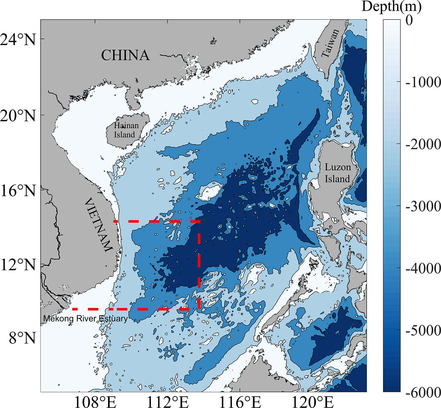
Figure 1 Bathymetry (m) of the SCS region. The red dashed box is the study area. The bathymetry data is obtained from ETOPO1.

2.2 SDD and environmental factors data

A total of 10 years (2010-2020) satellite-derived monthly SDD data are obtained from the Satco2 (http://www.geodata.cn). The spatial resolution of the data is 1.8 km. Previous studies have used this dataset to conduct research on marine elements in the SCS. The relationship model between SDD and water inherent optics is expressed as follows (He et al., 2014; He et al., 2017):

$\begin{array}{ll}\begin{array}{c}{Z}_d=0.25(a+b_b)\ln [\frac{{\rho }_{\rho }\alpha \beta (a+b_b)}{(C_{a}f{b}_b)}]\end{array}& (1)\end{array}$

where ρ_ρ is the surface reflectance of the transparency disk, α is the refraction factor, β is the water surface reflection factor, C_a is the ratio threshold, f is a variable ranging from 0.32 to 0.37, a is the absorption coefficient, and b_b is the backscattering coefficient. For case I water, a and b are estimated as follows:

$\begin{array}{ll}\begin{array}{c}a(\lambda )=[a_w(\lambda )+0.06A(\lambda )Ch{l}^{0.65}][1+0.2e^{-0.014(\lambda -440)}]\end{array}& (2)\end{array}$

$\begin{array}{ll}\begin{array}{c}{b}_b(\lambda )=b_{bw}(\lambda )+[0.3Ch{l}^{0.62}-b_w(550)]\left\{0.002+0.02[0.2-0.25\log (Chl)\frac{550}{\lambda }]\right\}\end{array}& (3)\end{array}$

where λ is the observation wavelength, a_w, b_w, and b_bw are the absorption, scattering and backscattering coefficients of pure water, respectively, and e is the Chl concentration. In addition, for case II water, the absorption (a_p) and scattering coefficient (b_bp) of suspended sediment should be increased on the basis of case I water:

$\begin{array}{ll}\begin{array}{c}{a}_p(\lambda )=s[0.025+0.038e^{-0.0055(\lambda -440)}]\end{array}& (4)\end{array}$

$\begin{array}{ll}\begin{array}{c}{b}_{bp}(\lambda )=0.019s[0.28-0.000167(\lambda -400)]\end{array}& (5)\end{array}$

where s is the concentration of suspended sediment.

SST, SSS and sea surface velocity data with a spatial resolution of 9 km (0.083°) are derived from global ocean reanalysis data simulated by The Copernicus Marine Environment Monitoring Service (CMEMS). The data extends from surface to 5500 m and is divided into 50 layers in the vertical direction. It adopts GEBCO data for layering nearshore and adopts ETOPO1 with a resolution of 1 arc minute to realize layering in the deep ocean, thus providing high-quality ocean environmental data (Wang et al., 2021).

The monthly average ocean wave and sea surface wind field data are derived from the ERA5 dataset of the European Center for Medium-Range Weather Forecasts (ECMWF). This dataset is the fifth-generation reanalysis dataset of global climate and weather over the past 40-70 years, including real-time updates from 1979 to the present. The dataset provides a large number of atmospheric, ocean wave and land surface parameters. The temporal resolution is hourly and monthly, and the spatial resolution of the reanalysis data is 0.25° (resolution of ocean wave data is 0.5°). The applicability of this product in the SCS has been verified and is in good agreement with buoy data (Shi et al., 2021).

The coastal upwelling region in the SCS is driven by classic wind-stressed Ekman dynamics (Zeng et al., 2022). In the upwelling region of southeastern Vietnam, Ekman transport along the shore (ETv) and offshore (ETu) and Ekman pumping (EPV) can transport nutrients from the coast or ocean bottom to the upper layer. This can promote the growth of phytoplankton and indirectly affect SDD. Ekman transport is calculated from wind components at 10 m above the sea surface (Equation 6, 7) (Cropper et al., 2014).

$\begin{array}{ll}\begin{array}{c}{Q}_x=\frac{{\rho }_a{C}_d}{\rho f}{(W_x^2+W_y^2)}^{\frac{1}{2}}{W}_x\end{array}& (6)\end{array}$

$\begin{array}{ll}\begin{array}{c}{Q}_y=-\frac{{\rho }_a{C}_d}{\rho f}{(W_x^2+W_y^2)}^{\frac{1}{2}}{W}_y\end{array}& (7)\end{array}$

where W is the wind speed near surface, $\rho$ is the sea water density (1025 kg/m³), and C_d is the dimensionless viscosity (1.4×10^-3). f is the Coriolis parameter, defined as twice the component of the angular velocity of earth (Ω) at latitude θ f = 2Ωsinθ. x and y correspond to the zonal and meridional components of wind, respectively.

EPV is calculated as follows:

$\begin{array}{ll}\begin{array}{c}EPV=\frac{curl(\tau )}{\rho f}\end{array}& (8)\end{array}$

where τ is surface wind stress.

The mixed layer depth (MLD) and barrier layer depth (BLD) distribution in the ocean is closely related to the internal motion of the ocean, marine organisms and marine meteorological elements. BLD is the water layer between the isothermal layer depth (ILD) and MLD, expressed as BLD=ILD-MLD. In this study, the gradient method is used to determine ILD and MLD. Different determination methods are used in offshore waters with a water depth of less than 200 m and in the open seas with larger water depths (Godfrey and Lindstrom, 1989; Chu et al., 2002):

offshore(≤200 m)

$\begin{array}{ll}\begin{array}{c}\frac{\partial T}{\partial z}=0.2°\text{C}·m^{-1} \frac{\partial {\sigma }_t}{\partial z}=0.1 kg·m^{-4} \end{array}& (9)\end{array}$

open sea(≥200 m)

$\begin{array}{ll}\begin{array}{c}\frac{\partial T}{\partial z}=0.05°\text{C}·m^{-1} \frac{\partial {\sigma }_t}{\partial z}=0.015 kg·m^{-4}\end{array}& (10)\end{array}$

where σt is the density of seawater obtained from temperature and salinity by TEOS10 (http://www.teos-10.org/), and T is sea water temperature.

2.3 Method

2.3.1 Empirical mode decomposition

Compared with the traditional wavelet analysis, the EMD proposed and improved by Huang can obtain more refined time-frequency local features. It smoothly processes complex signals and extracts the fluctuation or trend components of different scales from the original sequence. The output is several intrinsic mode functions (IMFs) of different scales and a trend item. The trend change characteristics have no relationship with past or future data. This method is widely used in atmospheric and oceanic research (Chen et al., 2013; Chen et al., 2014).

IMFs must satisfy two conditions (Huang et al., 1998). (a) The number of extreme points and zero crossing points throughout the data should be less than or equal to 1. (b) Any point where the mean of the envelope is defined by the local maximum or local minimum is 0. An IMF that meets these conditions has amplitude and frequency that vary as a function of time. EMD is ultimately decomposed into IMFs, and a residual term r(n) is obtained:

$\begin{array}{ll}\begin{array}{c}X(t)=\sum _{i=1}^{n}IM{F}_i+r(n)\end{array}& (11)\end{array}$

where X(t) is decomposed by EMD to obtain several IMFs. Based on the Hilbert transformation of each IMF, the instantaneous frequency and instantaneous amplitude of each component are obtained. For any signal X(t), it can be expressed as:

$\begin{array}{ll}\begin{array}{c}H(X(t))=y(t)=\frac{1}{\pi }pv{\int }^{}\frac{X(u)}{t-u}du\end{array}& (12)\end{array}$

In the above equation, pv is the Cauchy’s principal value, and the analytic signal corresponding to X(t) is:

$\begin{array}{ll}\begin{array}{c}Z(t)=X(t)+iy(t)=a(t)e^{i\theta (t)}\end{array}& (13)\end{array}$

where a(t) and θ(t) are the instantaneous amplitude and instantaneous phase of the signal, respectively, expressed as

$\begin{array}{ll}\begin{array}{c}a(t)=\sqrt{X{(t)}^2+y{(t)}^2}\end{array}& (14)\end{array}$

$\begin{array}{ll}\begin{array}{c}\theta (t)=arctan(\frac{y(t)}{X(t)})\end{array}& (15)\end{array}$

Further derivation of θ (t) function obtained from the original analysis signal yields the instantaneous frequency of the signal as follows:

$\begin{array}{ll}\begin{array}{c}\omega (t)=\frac{d\theta (t)}{dt}\end{array}& (16)\end{array}$

If the amplitude is plotted on the plane of time and frequency, the Hilbert spectrum of the original signal X(t) can be obtained.

This study mainly uses EMD to carry out multi-scale analysis and correlation analysis on the time series of SDD and related influencing factors in the study area. The Hilbert spectrum analysis is then applied to the obtained IMF modal components to finally obtain the Hilbert spectrum with clear physical meaning. This method can better describe the non-linear process and can effectively obtain the variation trend characteristics of SDD in different and multiple periods, in order to further determine the contribution of various environmental factors.

2.3.2 Generalized additive models

GAM is an important achievement in statistical research in recent years (Guisan et al., 2002). Its advantage is that it can explain the highly non-linear or monotonic relationship between response variables and environmental factors. The model is data-driven rather than assuming specific parameters between data in advance. It has high flexibility and can better explain the relationship between the response variable and the explanatory variable, and the importance of each explanatory variable. GAM can be expressed as:

$\begin{array}{ll}\begin{array}{c}g(Y)= \alpha + \sum _i^n{f}_i(x_i)+ϵ\end{array}& (17)\end{array}$

where $g(Y)$ is the connection function of the response variable SDD (the data of the response variable can be of any exponential distribution form), $\alpha$ is the intercept, $ϵ$ is the residual, n is the number of parameters, X_i is the ith explanatory variable, and $f_i(x_i)$ is the smoothing function used to describe the relationship between $g(Y)$ and the ith explanatory variable.

This study used the effective degree of freedom (EDF), P-value, deviance explained (D-E) and F-statistic to characterize the quality of the model’s statistical results. In addition, the larger the F-statistic, the higher the importance of the corresponding variable. When EDF=1, it represents a linear relationship between the variables and when EDF > 1, it indicates that the function is a non-linear curve equation. The larger the EDF, the more significant the non-linear relationship (Requia et al., 2019). P-value represents the significance level of the statistical results, D-E represent the model’s interpretation rate for the change of the response variable, and values closer to 1 mean that the model works better.

Based on the inversion principle of SDD, generally, the factors that most directly affect SDD include SPM, chlorophyll and CDOM. In contrast, other environmental factors indirectly affect SDD by affecting the spatial and temporal distribution of the above three environmental factors. In this study, one environmental factor is selected as the explanatory variable of GAM each time, and the relationship and contribution of each factor to SDD changes are analyzed. The environmental variables include SSS, SST, ET (Ekman transport), EPV, CV (current velocity), ILD, BLD, wind and nine wave parameters:mean direction of total swell, significant height of total swell, mean period of total swell, MDWW (mean direction of wind waves), mean period of wind waves, mean wave direction, mean wave period, SWH (significant height of combined wind waves and swell), and significant height of wind waves. The construction and data analysis of the GAM model are completed using the R mgcv package.

3 Results

3.1 Spatial distribution and variation characteristics of SDD

The monthly mean SDD in the study area from 2011 to 2020, shows the variation range of the monthly mean SDD in the study area is 26.6~34.9 m during the 10 years (Figure 2). SDD has obvious seasonal variation characteristics, reaching a maximum in May, decreasing rapidly, and reaching a minimum in August each year. Concretely, the average SDD in June (summer) is 32.4 m, when the water clarity of the study area is higher, but it was still very low in September, which was already autumn (mean SDD value is 28.6 m). Apparently, the most turbid time of the year is July to September.

FIGURE 2

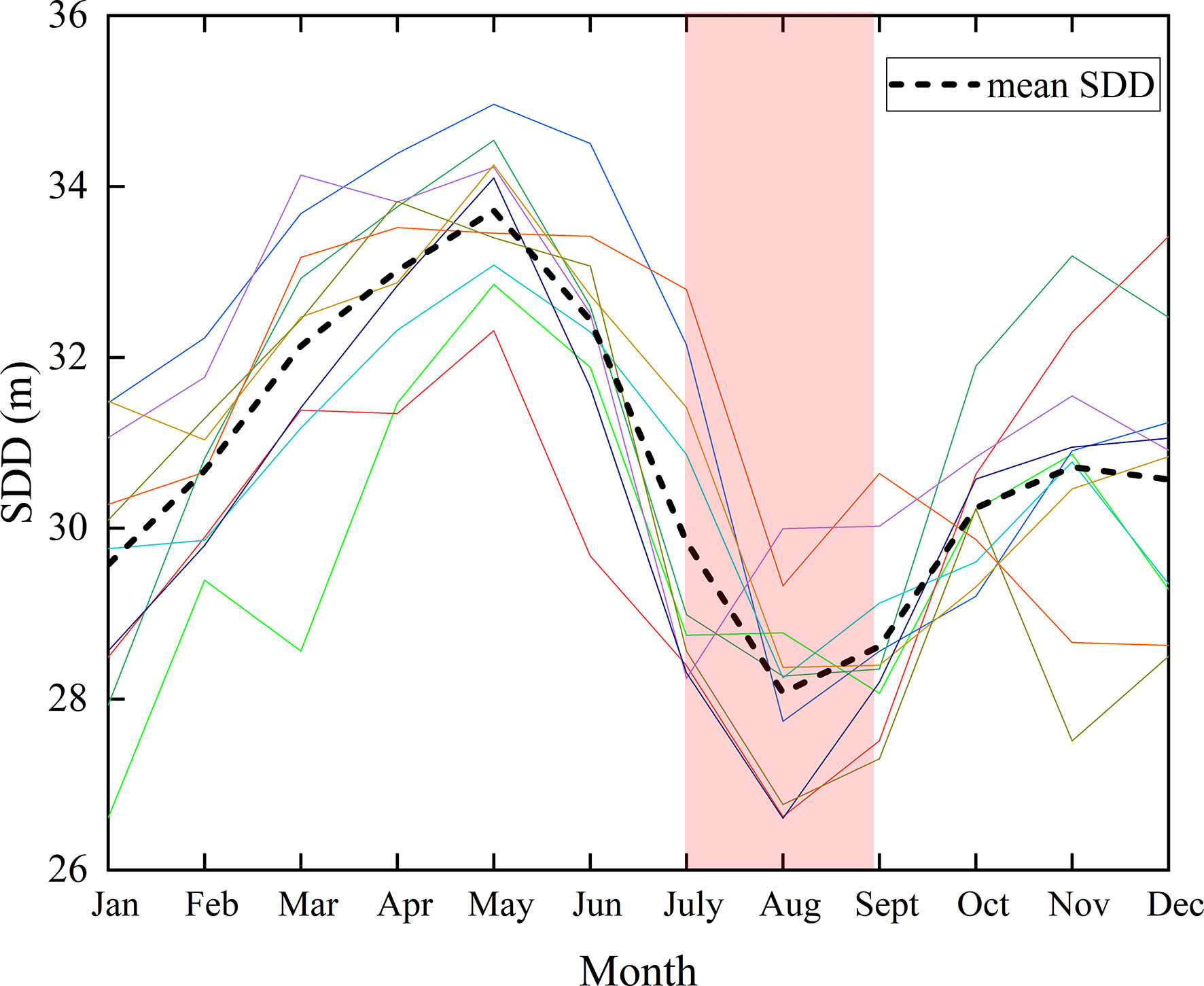
Figure 2 Annual cycle of SDD calculated from 2011 to 2020 in the study area. Different color lines represent the SDD of different years. Black dashed line represents the mean value of SDD. The red area represents the low value of SDD from July to September.

We average the SDD in the SCS and surrounding seas by season according to the monthly variation characteristics of SDD (Figure 3), in order to better understand the spatial and temporal distribution of SDD from 2011 to 2020. Note that the definition of the four seasons is delayed by one month compared to the commonly used time, e.g., summer is July-September. This approach has been applied in previous studies related to primary productivity in SCS (Zhao and Wang, 2018), so we consider it acceptable in studies of SDD directly related to primary productivity. Overall, SDD have a gradient change in spatial distribution, and the SDD pattern is basically the same along the coast. More SDD low-value areas are distributed in the near shore and estuarine areas. According to the seasonal average distribution, the average value of SDD from July to September is significantly lower than in other sea areas (Figure 3C). The main axis of the low-value area is parallel to the southern coastline of the Indo-China Peninsula, showing tongue-shaped, which seems to be an extension of the low-value area of the Mekong Estuary. This phenomenon does not appear in other seasons (Figures 3A, B, D).

FIGURE 3

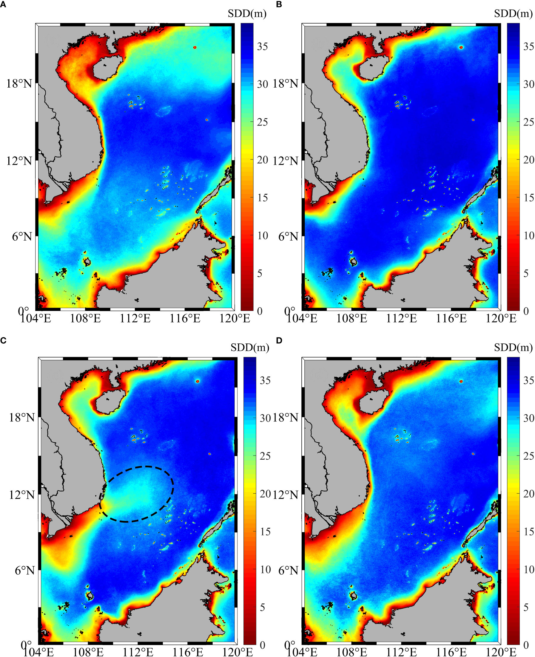
Figure 3 Distributions of mean SDD (background color, m) for (A) January-March (B) April-June (C) July-September (D) October-December from 2011-2020. The dotted line is the low value area of SDD.

3.2 Multi-scale analysis of SDD

Taking the monthly time series of SDD in the study area from 2011 to 2020 with a total of 120 sample points, the SDD is decomposed by the EMD method (Figure 4). The plot shows the EMD decomposition result of SDD monthly average value, where ORG is the original time series of SDD, IMF1-5 are the five signal components, which reflect the SDD fluctuation characteristics of different time scales from high frequency to low frequency, and trend denotes the trend term. In addition, the period of each component is calculated by the distance between adjacent maximum (minimum) values, and the average value and variance of each component. The average periods of IMF1-5 components are 6 months, 11 months, 16 months, 24 months, and 60 months, respectively.

FIGURE 4

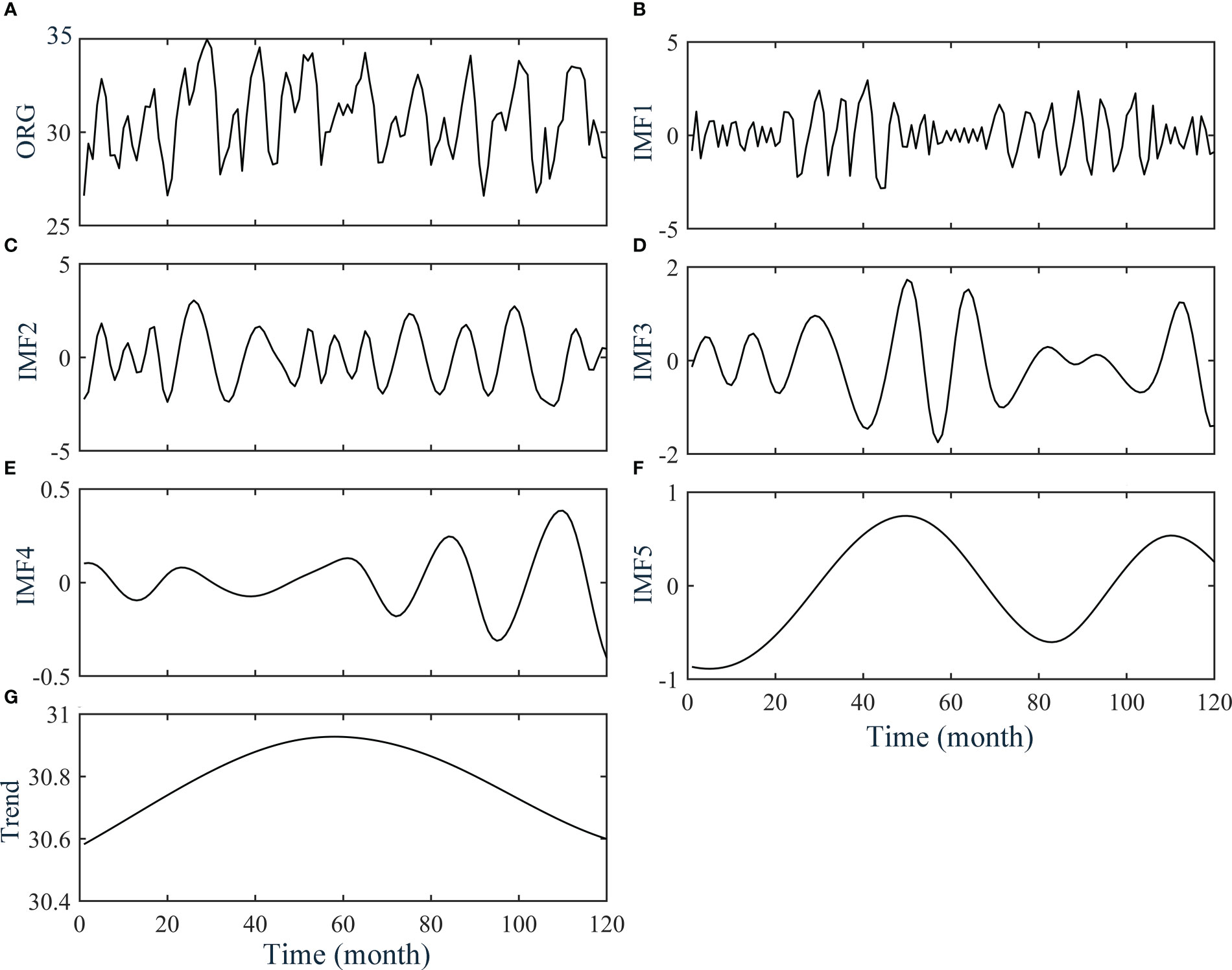
Figure 4 Decomposition results of SDD time series using the EMD. (A) is original component, (B–F) are IMFs, and (G) is the trend component.

Specifically, the first signal component (IMF1) of SDD indicated an aperiodic oscillation, it contains a high-frequency oscillation process. During 0-20 months and 50-70 months, the amplitude of SDD changes is about 1.5 m, and the amplitude can reach 4.7 m in other time intervals. IMF2 is the interannual component expressing the interannual variation process, and its maximum amplitude is 4.4 m. IMF3 is a component with a period of 16 months. Its amplitude is larger between 50 and 70 months, which may be caused by low-frequency anomalous events in the corresponding period. IMF4 represents SDD changes on a time scale of about two years, with smaller changes in amplitude. The variation characteristics of IMF5 are relatively gentle, with a low-frequency variation signal on the five-year time scale. The last signal component (Trend) is a non-monotonic signal. SDD first increases and then decreases during the ten years. It reaches a maximum of 34.96 m around the 60th month and decreases in the next five years. The SDD remains at 30.5~31 m during the ten years.

In order to analyze the variation characteristics of SDD, the Hilbert transform is performed on the IMF1-5 components of SDD signal. The time spectrum of the signal is plotted in Figure 5. Signals with average frequencies around 0.08/month and 0.15/month fluctuate widely, while low-frequency signals (less than 0.05/month) exhibit a near-stationary band. In terms of energy distribution, high energy is mostly distributed in higher frequency signals, which indicates that the SDD in the study area has the largest fluctuations on the time scale of about half a year to one year. This further confirms the signal analysis in Figure 4.

FIGURE 5

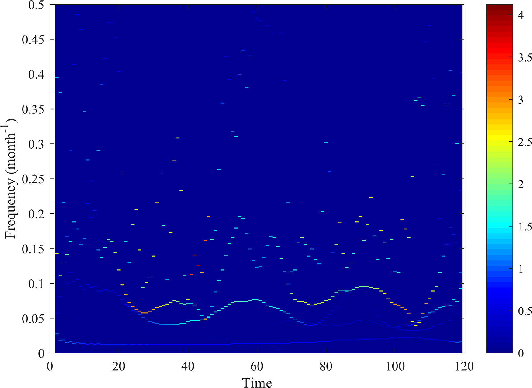
Figure 5 Hilbert-Huang spectrum analysis of SDD. The color represents the energy value, where the higher the value, the higher the energy event.

3.3 GAM analysis of SDD and environmental factors

According to the principle of SDD inversion calculation and the actual situation of the study area, the significant reduction in SDD phenomenon is often caused by the joint action of various influencing factors (Gordon et al., 1975);. Therefore, we include multiple oceanographic and meteorological elements in the analysis, use the variance inflation factor standard to eliminate the multi-collinearity environmental factors (Wood, 2004). Finally, SSS, SST, MDWW, SWH, ETu, ETv, BLD, EPV, Cu (offshore current), Cv (alongshore current), MLD, WD, and ILD environmental factors are screened as explanatory variables.

The GAM results shows that the combined explanation rate of the model is 72.1%, and all selected driving factors significantly affect the changes in SDD at P-value< 0.01, which were all statistically significant. The environmental factors that explain the SDD variation with a high rate (15.3%-38.2%) with effects ranked as SSS > Cu > WD > ETu > SST > MDWW, and they fit well with the model equations constructed by SDD (Table 1). Although the rest of the factors pass the P-value significance test, their explanatory power for SDD changes is relatively low (less than 15%) and the model fit is also poor. In addition, the EDF of each explanatory variable is greater than 1, indicating that the constructed function is a non-linear equation and there is a significant non-linear relationship between the explanatory variables and SDD.

TABLE 1

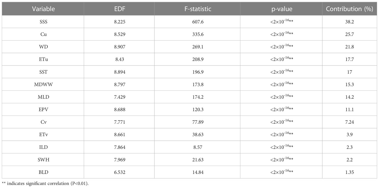
Table 1 GAM fitting results of SDD and environmental factors.

The smooth regression function of related environmental factors is calculated using the GAM model established between multiple driving factors and SDD response variables. The effect diagram of the impact of environmental factors on SDD changes with an explanation rate greater than 15% is obtained (Figure 6). The gray shading in the figure represents the upper and lower bounds of the confidence interval, and the solid line represents the smooth fitting curve.

FIGURE 6

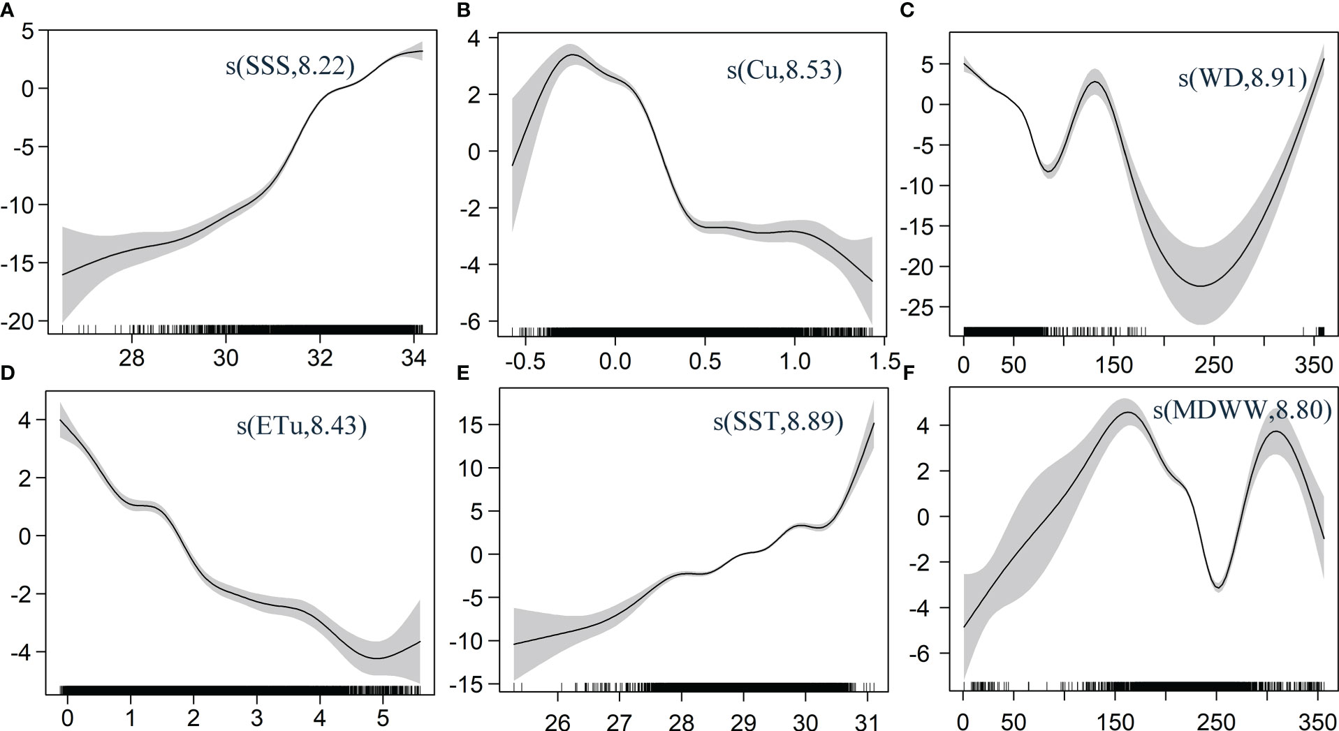
Figure 6 Response curves of SDD to changes in (A) SSS, (B) Cu, (C) WD, (D) ETu, (E)SST and (F) MDWW. The Y-axis in each subplot represents the smoothing function term for each factor, and the numbers in brackets represent degrees of freedom.

According to the results, each environmental factor shows a non-linear relationship with the change in SDD. Specifically, SDD is positively correlated with SSS and SST. When SSS is 30.5-31.5 PSU and SST is 28-30.5 °C, the confidence interval is small and the reliability is high. In addition, SSS and SST have the most significant impact on SDD (Figures 6A, E). Cu and ETu have similar effects on SDD, with a general decrease in SDD as Cu and ETu increase (Figures 6B, D). It should be noted that when Cu is greater than 0.5 m/s, SDD reaches the minimum, and then there is no obvious trend, indicating that the response of SDD to Cu in the study area is phased and does not decrease with the increase in Cu. The relationship between WD and SDD is diverse. SDD is relatively high when WD is 0-90° and the confidence interval is small (Figure 6C). SDD increases with the increase in WD in this interval. When WD is between 90° and 230°, SDD first rises and then falls, reaching two peaks at 130° and 230°, respectively. SDD increases with the increase of WD. The relationship between MDWW and SDD is complex (Figure 6F). MDWW and SDD are positively correlated when the wave direction is between 0 and 180°. When MDWW is between 180° and 290°, SDD decreases and then increases. The SDD in the interval is significantly affected by MDWW. When MDWW is greater than 290°, SDD decreases again.

4 Discussion

4.1 Multi-scale correlation analysis of SDD and main environmental factors

In this paper, EMD is used to objectively deal with nonlinear and nonsmooth processes. We perform EMD transformations on the main factors obtained from the GAM and analyze their response to changes in SDD at different time scales. Based on the EMD signal decomposition, we use the Pearson correlation coefficient to analyze the correlation between SDD and various influencing factors on multiple time scales to obtain the contribution of the correlation factors that affect SDD changes on different time scales (Figure 7).

FIGURE 7

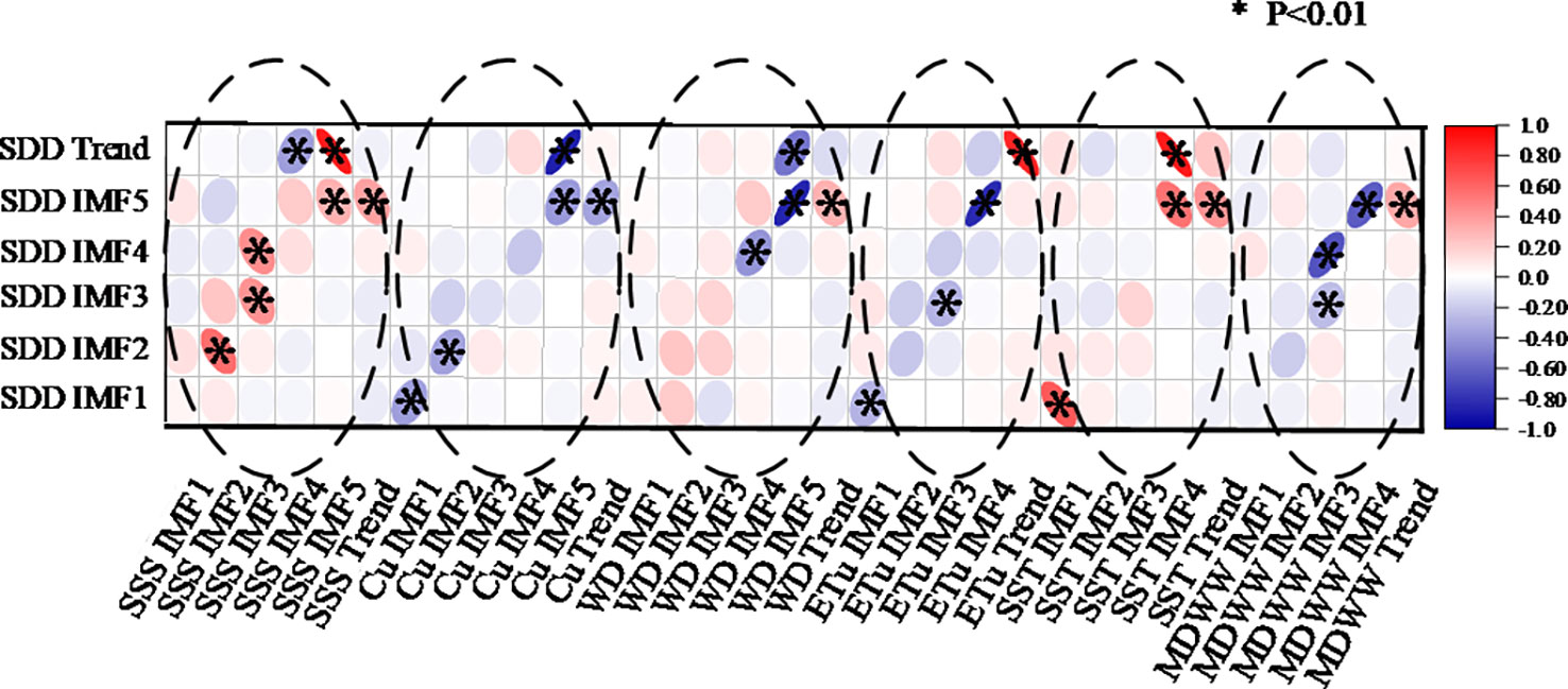
Figure 7 Correlation analysis of SDD and environmental factors at various time scales. The shape and color of the ellipse in the figure represent the degree of the correlation, the direction of the ellipse represents positive or negative correlation, and * means that the data has been tested for significance at 0.01.

Specifically, with the exception of SDD IMF1, SSS has a regulating effect on all SDD signal components with a period greater than or equal to 11 months, and the correlation coefficients of the two can reach 0.565, 0.429, 0.444, 0.315, and 0.883, respectively, which indicates that SDD is significantly driven by SSS on interannual or longer time scales, and they are positively correlated. Cu has a significant negative correlation with SDD period of less than 11 months and signal components greater than 60 months, which means that SDD is affected on short time scales within 1 year and long time scales greater than 5 years. WD is similar to MDWW, both of which have a moderate effect on SDD changes greater than 16 months. The effects of ETu and SST exist mainly on longer time scales (Based on available theoretical and GAM results, ETu is negatively correlated with SDD, so the positive correlation results between SDD Trend and ETu Trend are not considered. The anomalous positive correlation of the long-term trend correlation may be related to the amount of data). In addition, they are both significantly correlated with SDD IMF1, which indicates that ETu and SST also have a non-negligible effect on the semiannual-scale SDD oscillation.

In general, SSS, Cu, ETu, and SST significantly impact SDD on a six-month to one-year scale. On a time scale of about two years (SDD IMF3, SDD IMF4), SDD is significantly driven by SSS, WD, ETu, and MDWW. All factors play a significant role in the approximately five-year scale signal of SDD. Therefore, we can conclude that SSS influences the signal components of SDD at five different time scales, indicating that SSS is an important environmental factor affecting SDD at most of the time. The modulating effect of SSS on SDD is the most comprehensive, followed by the effect of Cu, which has an important impact on the four signal components of SDD.

4.2 Analysis of the response mechanism of SDD to environmental factors

According to the distribution of SSS and SST, it can be concluded that the study sea area is characterized by low temperature and low salinity. The Mekong River brings a large number of low-salinity plumes during the rainy season, which makes the estuary and its adjacent waters low in salt content (SSS minimum is below 22 PSU) (Figure 8A) (Hordoir et al., 2006). Based on our results, there is a significant positive correlation between SSS and SDD. SDD decreases with the decrease in SSS, and appropriate salinity promotes the mass growth and reproduction of phytoplankton, thereby reducing the transparency of seawater (Jeppesen et al., 2007). At the same time, part of the study area is in the upwelling region, and the distribution of SST shows the cold spot phenomenon near shore (Wang et al., 2013; Dang et al., 2022). This is due to the deep cold water brought by the upwelling, causing the SST in the upwelling area to be less than 26.5 °C at minimum (Figure 8E). Based on the Pearson analysis between the GAM analysis and EMD, SST and SDD are positively correlated. The decrease in SST reduces the thickness of the thermocline and the vertical stability of seawater. Nutrients are more easily mixed, so SDD decreases as SST decreases. It is worth noting that due to the strong seasonal changes in SST, the changes to the marine biological environment are relatively slow, so the impact of SST on SDD is mainly reflected on a longer time scale in addition to the semi-annual scale. In short, the upwelling sea area carries a large amount of nutrients and SPM (Li et al., 2015). It can be concluded that the plume and upwelling of the Mekong River affect the distribution of SSS and SST, which indirectly causes the SDD in the study area to decrease significantly.

FIGURE 8

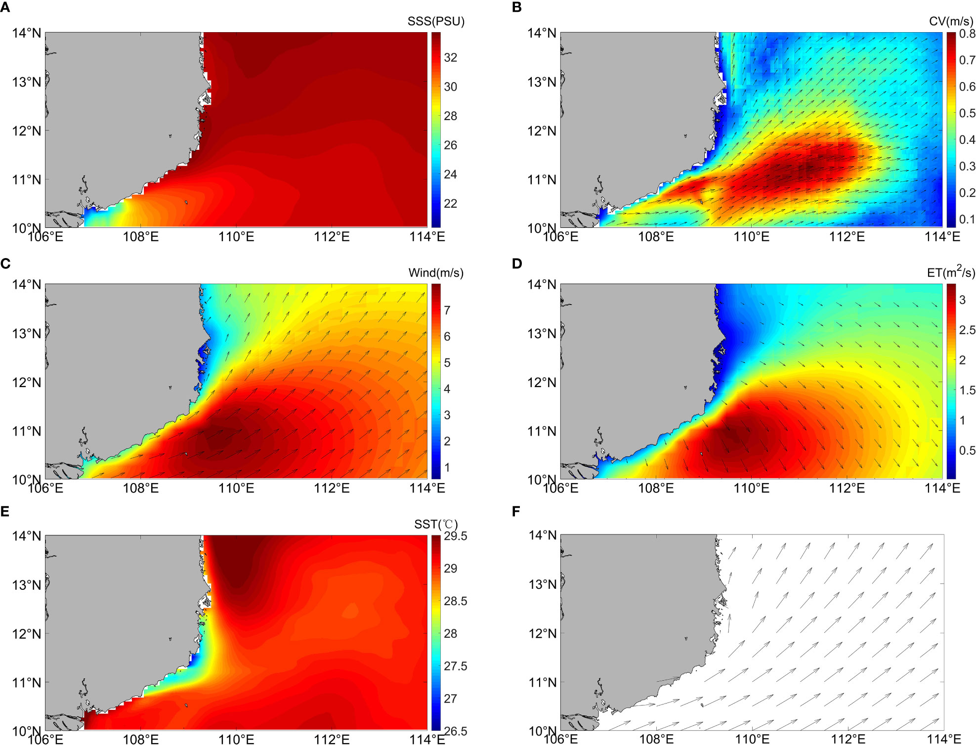
Figure 8 Spatial distribution of (A) SSS; (B) Cu; (C) WD; (D) ET; (E) SST; (F) MDWW. (July to September).

In marine systems, regional SDD is sensitive to hydrodynamic and meteorological conditions (Zhou et al., 2022). WD from July to September is mostly southwesterly (Figure 8C), and the distribution of the wind stress curl field is favorable to the formation of summertime eastward jet (Sun and Lan, 2021), which has a significant impact on the regional climate and ecological environment. The summertime eastward jet generally intensifies in July, reaches its maximum in August, and then gradually weakens in September, which is consistent with the appearance of the low value region of SDD. As shown in the distribution of the sea surface current field (Figure 8B), the prevailing southwest wind promotes Cu in the offshore direction, which increases the intensity of Cu in the study area and promotes the transfer of low salinity cold water from the Mekong River to the east, thus indirectly causing significantly low SDD (Van Der Woerd and Pasterkamp, 2008). Cu can lead to the summertime Chl-a jet phenomenon (Chl-a concentrations above 0.13 mg m^-3) (Zeng et al., 2022), which can have a direct impact on SDD. In addition, Cu driven by wind also has periodic changes due to seasonal changes in WD. Therefore, Cu impacts the variation of SDD on a semi-annual to annual scale. Another environmental factor driven by wind, MDWW, also plays a role in SDD. MDWW is mostly southwestern from July to September (Figure 8F). The GAM model results show that SDD is significantly lower when the direction of weaves is 180-270° due to MDWW transporting more nutrients with SPM and contributed to the reduction of SDD. Finally, Ekman transport, as one of the environmental variables affecting SDD, is also driven by wind (Dippner et al., 2007; Wang et al., 2013). The offshore direction of ET in the study area is southeast and perpendicular to the shoreline (Figure 8D), favoring the creation of more phytoplankton growth and causing a decrease in SDD.

It is noteworthy that each environmental factor we analyzed acts indirectly on SDD by affecting chlorophyll or SPM. The sources of chlorophyll, representing primary productivity, are nearshore transport and locally generated (Liu and Tang, 2022), which affect SDD through physical and biological processes. Both summertime eastward jet and upwelling significantly affect local chlorophyll, which explains the relationship between SDD response to EPV intensity and summertime eastward jet in the GAM analysis, i.e., these processes are significantly associated with changes in SDD, but their contribution to SDD changes is limited due to seasonal fluctuations in EPV and hydrodynamics. The effect of MLD on SDD is similar to the EPV effect. MLD is influenced by monsoons and eddies, especially in summer when the MLD increases and phytoplankton can obtain abundant nutrients in surface waters, which has a great impact on local SDD. However, due to its seasonal variation, the effect of MLD on SDD is limited during the whole year.

5 Conclusions

In this study, we use multi-source satellite remote sensing data and reanalysis data to study the spatial distribution and variation characteristics of SDD in the study area (10°~14°E, 105°~114°N) from 2011 to 2020. The monthly mean time series shows that the SDD values in the study area are bimodal and varied significantly seasonally, with the highest and lowest values occurring in May and August each year, respectively. The spatial and temporal distributions show a distinct zone of low SDD values (average 28.8 m) from July to September each year compared to nearby waters, with its main axis parallel to the southern shoreline of the Mekong estuary in a tongue shape.

To explore the SDD low value phenomenon, a non-parametric model, GAM, is used to identify the dominant environmental factors affecting SDD variation and analyze the relationship between the dominant environmental factors and SDD variation. The combined explanation rate of the model is 72.1%, and the environmental factors’ influence contribution is ranked SSS > Cu > WD > ETu > SST > MDWW, with different degrees of nonlinear response relationships. Among them, SDD is positively correlated with SSS and SST, and negatively correlated with Cu and ETu. Moreover, in order to explore at what time scales environmental factors influence SDD, this paper performs an EMD decomposition of the main environmental factors. The analysis results show that the variation of SSS, Cu, ETu, and SST on the interannual scale have important effects on SDD, while on longer time scales, SSS, Cu, WD, and SST had effects on SDD. In general, SSS has the largest comprehensive impact on SDD. WD is also an important segment that can indirectly affect SDD by altering ocean dynamic processes.

Data availability statement

The raw data supporting the conclusions of this article will be made available by the authors, without undue reservation.

Author contributions

YS: data analysis, writing and editing. YS and YX: figure plotting. DL and GX: conceptualization, methodology and reviewing. All authors contributed to the article and approved the submitted version.

Funding

This research is supported by the project supported by Southern Marine Science and Engineering Guangdong Laboraory (Zhuhai) (SML2020SP007), the Guangdong Basic and Applied Basic Research Foundation (2019A1515110840), and the Research Startup Foundation of Guangdong Ocean University (R20009).

Acknowledgments

Thanks to the SDD data support from “National Earth System Science Data Sharing Infrastructure, National Science & Technology Infrastructure of China. (http://www.geodata.cn)”; Thanks to the SDD data support from “National Earth System Science Data Sharing Infrastructure, National Science & Technology Infrastructure of China. (http://www.geodata.cn)” the Copernicus for providing the monthly SST, SSS, and ocean current data; the ECMWF for providing the wave and wind data. Thanks to Dr. Kenny T.C. Lim Kam Sian for the contributions to this manuscript.

Conflict of interest

The authors declare that the research was conducted in the absence of any commercial or financial relationships that could be construed as a potential conflict of interest.

Publisher’s note

All claims expressed in this article are solely those of the authors and do not necessarily represent those of their affiliated organizations, or those of the publisher, the editors and the reviewers. Any product that may be evaluated in this article, or claim that may be made by its manufacturer, is not guaranteed or endorsed by the publisher.

References

Aas E., Høkedal J., Sørensen K. (2014). Secchi depth in the oslofjord–skagerrak area: theory, experiments and relationships to other quantities. Ocean Sci. 10 (2), 177–199. doi: 10.3390/rs11192226

CrossRef Full Text | Google Scholar

Alsahli M. M., Nazeer M. (2021). Spatiotemporal variability of secchi depths of the north Arabian gulf over the last two decades. Estuar. Coast. Shelf Sci. 260, 107487. doi: 10.1016/j.ecss.2021.107487

CrossRef Full Text | Google Scholar

Bohn V. Y., Carmona F., Rivas R., Lagomarsino L., Diovisalvi N., Zagarese H. E. (2018). Development of an empirical model for chlorophyll-a and secchi disk depth estimation for a pampean shallow lake (Argentina). Egypt. J. Remote Sens. Space Sci. 21 (2), 183–191. doi: 10.1016/j.ejrs.2017.04.005

CrossRef Full Text | Google Scholar

Cai S., Long X., Wang S. (2007). A model study of the summer southeast Vietnam offshore current in the southern south China Sea. Cont. Shelf Res. 27 (18), 2357–2372. doi: 10.1016/j.csr.2007.06.002

CrossRef Full Text | Google Scholar

Chang C. W. J., Hsu H. H., Wu C. R., Sheu W. J. (2008). Interannual mode of sea level in the south China Sea and the roles of El Niño and El Niño modoki. Geophys. Res. Lett. 35 (3), L03601. doi: 10.1029/2007GL032562

CrossRef Full Text | Google Scholar

Chen X., Feng Y., Huang N. E. (2014). Global sea level trend during 1993–2012. Glob. Planet Change 112, 26–32. doi: 10.1016/j.gloplacha.2013.11.001

CrossRef Full Text | Google Scholar

Chen X., Zhang Y., Zhang M., Feng Y., Wu Z., Qiao F., et al. (2013). Intercomparison between observed and simulated variability in global ocean heat content using empirical mode decomposition, part I: modulated annual cycle. Clim. Dyn. 41 (11), 2797–2815. doi: 10.1007/s00382-012-1554-2

CrossRef Full Text | Google Scholar

Chu P. C., Liu Q., Jia Y., Fan C. (2002). Evidence of a barrier layer in the sulu and celebes seas. J. Phys. Oceanogr. 32 (11), 3299–3309. doi: 10.1175/1520-0485(2002)032<3299:EOABLI>2.0.CO;2

CrossRef Full Text | Google Scholar

Cloern J. E. (1987). Turbidity as a control on phytoplankton biomass and productivity in estuaries. Cont. Shelf Res. 7, 1367–1381. doi: 10.1016/0278-4343(87)90042-2

CrossRef Full Text | Google Scholar

Cropper T. E., Hanna E., Bigg G. R. (2014). Spatial and temporal seasonal trends in coastal upwelling off Northwest Africa 1981–2012. Deep. Res. Part I Oceanogr. Res. Pap. 86, 94–111. doi: 10.1016/j.dsr.2014.01.007

CrossRef Full Text | Google Scholar

Dang X., Bai Y., Gong F., Chen X., Zhu Q., Huang H., et al. (2022). Different responses of phytoplankton to the ENSO in two upwelling systems of the south China Sea. Estuar. Coasts. 45 (2), 485–500. doi: 10.1007/s12237-021-00987-2

CrossRef Full Text | Google Scholar

Dippner J. W., Nguyen K. V., Hein H., Ohde T., Loick N. (2007). Monsoon-induced upwelling off the Vietnamese coast. Ocean Dynam. 57 (1), 46–62. doi: 10.1007/s10236-006-0091-0

CrossRef Full Text | Google Scholar

Duy Vinh V., Ouillon S., Van Thao N., Ngoc Tien N. (2016). Numerical simulations of suspended sediment dynamics due to seasonal forcing in the Mekong coastal area. Water 8 (6), 255. doi: 10.3390/w8060255

CrossRef Full Text | Google Scholar

Erlandsson C. P., Stigebrandt A. (2006). Increased utility of the secchi disk to assess eutrophication in coastal waters with freshwater run-off. J. Mar. Syst. 60, 19–29. doi: 10.1016/j.jmarsys.2005.12.001

CrossRef Full Text | Google Scholar

Godfrey J. S., Lindstrom E. J. (1989). The heat budget of the equatorial western pacific surface mixed layer. J. Geophys. Res. Oceans 94 (C6), 8007–8017. doi: 10.1029/JC094iC06p08007

CrossRef Full Text | Google Scholar

Gordon H. R., Brown O. B., Jacobs M. M. (1975). Computed relationships between the inherent and apparent optical properties of a flat homogeneous ocean. Appl. Opt. 14 (2), 417–427. doi: 10.1364/AO.14.000417

CrossRef Full Text | Google Scholar

Gordon H., Clark D., Brown J., Brown O., Evans R., Broenkow W. (1983). Phytoplankton pigment concentrations in the middle Atlantic bight: comparison between ship determinations and coastal zone color scanner estimates. Appl. Opt. 22, 20–36. doi: 10.1364/AO.22.000020

CrossRef Full Text | Google Scholar

Guisan A., Edwards T. C. Jr., Hastie T. (2002). Generalized linear and generalized additive models in studies of species distributions: Setting the scene. Ecol. Modell. 157 (2-3), 89–100. doi: 10.1016/S0304-3800(02)00204-1

CrossRef Full Text | Google Scholar

Harvey E. T., Walve J., Andersson A., Karlson B., Kratzer S. (2019). The effect of optical properties on secchi depth and implications for eutrophication management. Front. Mar. Sci. 5. doi: 10.3389/fmars.2018.00496

CrossRef Full Text | Google Scholar

Hayami Y., Maeda K., Hamada T. (2015). Long term variation in transparency in the inner area of ariake Sea. Estuar. Coast. Shelf Sci. 163, 290–296. doi: 10.1016/j.ecss.2014.11.029

CrossRef Full Text | Google Scholar

He X., Bai Y., Chen C. T. A., Hsin Y. C., Wu C. R., Zhai W., et al. (2014). Satellite views of the episodic terrestrial material transport to the southern Okinawa trough driven by typhoon. J. Geophys. Res. Oceans 119 (7), 4490–4504. doi: 10.1002/2014JC009872

CrossRef Full Text | Google Scholar

He X., Pan D., Bai Y., Wang T., Chen C. T. A., Zhu Q., et al. (2017). Recent changes of global ocean transparency observed by SeaWiFS. Cont. Shelf Res. 143, 159–166. doi: 10.1016/j.csr.2016.09.011

CrossRef Full Text | Google Scholar

Hordoir R., Nguyen K. D., Polcher J. (2006). Simulating tropical river plumes, a set of parametrizations based on macroscale data: A test case in the Mekong delta region. J. Geophys. Res. Oceans 111, C09036. doi: 10.1029/2005JC003392

CrossRef Full Text | Google Scholar

Huang N. E., Shen Z., Long S. R., Wu M. C., Shih E. H., Zheng Q., et al. (1998). The empirical mode decomposition and the Hilbert spectrum for non stationary time series analysis. Proc. R. Soc Lond. 454, 903–995. doi: 10.1098/rspa.1998.0193

CrossRef Full Text | Google Scholar

Idris M. S., Siang H. L., Amin R. M., Sidik M. J. (2022). Two-decade dynamics of MODIS-derived secchi depth in peninsula Malaysia waters. J. Mar. Syst. 236, 103799. doi: 10.1016/j.jmarsys.2022.103799

CrossRef Full Text | Google Scholar

Jeppesen E., Søndergaard M., Pedersen A. R., Jürgens K., Strzelczak A., Lauridsen T. L., et al. (2007). Salinity induced regime shift in shallow brackish lagoons. Ecosystems 10 (1), 48–58. doi: 10.1007/s10021-006-9007-6

CrossRef Full Text | Google Scholar

Kirk J. T. O. (1994). Light and photosynthesis in aquatic ecosystems. 2nd ed (Cambridge, UK: Cambridge University Press).

Google Scholar

Klemas V. (2012). Remote sensing of algal blooms: An overview with case studies. J. Coast. Res. 28 (1A), 34–43. doi: 10.2112/JCOASTRES-D-11-00051.1

CrossRef Full Text | Google Scholar

Li Y., Xu X., Yin X., Fang J., Hu W., Chen J. (2015). Remote-sensing observations of typhoon soulik, (2013) forced upwelling and sediment transport enhancement in the northern Taiwan strait. Int. J. Remote Sens. 36 (8), 2201–2218. doi: 10.1080/01431161.2015.1035407

CrossRef Full Text | Google Scholar

Li J., Yu Q., Tian Y. Q., Becker B. L. (2017). Remote sensing estimation of colored dissolved organic matter (CDOM) in optically shallow waters. ISPRS J. Photog. Remote Sens. 128, 98–110. doi: 10.1016/j.isprsjprs.2017.03.015

CrossRef Full Text | Google Scholar

Liu F., Tang S. (2022). A double-peak intraseasonal pattern in the chlorophyll concentration associated with summer upwelling andmesoscale eddies in the western south China Sea. J. Geophys. Res. Oceans 127 (1), e2021JC017402. doi: 10.1029/2021JC017402

CrossRef Full Text | Google Scholar

Luis K. M., Rheuban J. E., Kavanaugh M. T., Glover D. M., Wei J., Lee Z., et al. (2019). Capturing coastal water clarity variability with landsat 8. Mar. Pollut. Bull. 145, 96–104. doi: 10.1016/j.marpolbul.2019.04.078

CrossRef Full Text | Google Scholar

Nishijima W., Umehara A., Sekito S., Okuda T., Nakai S. (2016). Spatial and temporal distributions of secchi depths and chlorophyll a concentrations in the suo Nada of the seto inland Sea, Japan, exposed to anthropogenic nutrient loading. Sci. Total Environ. 571, 543–550. doi: 10.1016/j.scitotenv.2016.07.020

CrossRef Full Text | Google Scholar

Nishijima W., Umehara A., Sekito S., Wang F., Okuda T., Nakai S. (2018). Determination and distribution of region-specific background secchi depth based on long-term monitoring data in the seto inland sea. Japan. Ecol. Indic. 84, 583–589. doi: 10.1016/j.ecolind.2017.09.014

CrossRef Full Text | Google Scholar

Philippart C., Salama M. S., Kromkamp J. C., van der Woerd H. J., Zuur A. F., Cadee G. C. (2013). Four decades of variability in turbidity in the western wadden Sea as derived from corrected secchi disk readings. J. Sea Res. 82, 67–79. doi: 10.1016/j.seares.2012.07.005

CrossRef Full Text | Google Scholar

Requia W. J., Jhun I., Coull B. A., Koutrakis P. (2019). Climate impact on ambient PM2. 5 elemental concentration in the united states: A trend analysis over the last 30 years. Environ. Int. 131, 104888. doi: 10.1016/j.envint.2019.05.082

CrossRef Full Text | Google Scholar

Rodrigues T., Alcântara E., Watanabe F., Imai N. (2017). Retrieval of secchi disk depth from a reservoir using a semi-analytical scheme. Remote Sens. Environ. 198, 213–228. doi: 10.1016/j.rse.2017.06.018

CrossRef Full Text | Google Scholar

Shi H., Cao X., Li Q., Li D., Sun J., You Z., et al. (2021). Evaluating the accuracy of ERA5 wave reanalysis in the water around China. J. Ocean Univ. China 20 (1), 1–9. doi: 10.3390/atmos13060935

CrossRef Full Text | Google Scholar

Sun Y., Lan J. (2021). Summertime eastward jet and its relationship with western boundary current in the south China Sea on the interannual scale. Clim. Dyn. 56 (3), 935–947. doi: 10.1007/s00382-020-05511-z

CrossRef Full Text | Google Scholar

Tang S., Chen C. (2016). Novel maximum carbon fixation rate algorithms for remote sensing of oceanic primary productivity. IEEE J. Selected. Topics. Appl. Earth Observ. Remote Sensing. 9 (11), 5202–5208. doi: 10.1109/JSTARS.2016.2574898

CrossRef Full Text | Google Scholar

Tang D. L., Kawamura H., Doan-Nhu H., Takahashi W. (2004). Remote sensing oceanography of a harmful algal bloom off the coast of southeastern Vietnam. J. Geophys. Res. Oceans 109, 2045. doi: 10.1029/2003JC002045

CrossRef Full Text | Google Scholar

Van Der Woerd H. J., Pasterkamp R. (2008). HYDROPT: A fast and flexible method to retrieve chlorophyll-a from multispectral satellite observations of optically complex coastal waters. Remote Sens. Environ. 112 (4), 1795–1807. doi: 10.1080/01431161.2015.1035407

CrossRef Full Text | Google Scholar

Wang H., Fu D., Liu D., Xiao X., He X., Liu B. (2021). Analysis and prediction of significant wave height in the beibu gulf, south China Sea. J. Geophys. Res. Oceans 126 (3), e2020JC017144. doi: 10.1029/2020JC017144

CrossRef Full Text | Google Scholar

Wang D., Gouhier T. C., Menge B. A., Ganguly A. R. (2015). Intensification and spatial homogenization of coastal upwelling under climate change. Nature 518, 390–394. doi: 10.1038/nature14235

CrossRef Full Text | Google Scholar

Wang F., Umehara A., Nakai S., Nishijima W. (2019). Distribution of region-specific background secchi depth in Tokyo bay and ise bay, Japan. Ecol. Indic. 98, 397–408. doi: 10.3390/rs11161948

CrossRef Full Text | Google Scholar

Wang D., Wang H., Li M., Liu G., Wu X. (2013). Role of ekman transport versus ekman pumping in driving summer upwelling in the south China Sea. J. Ocean Univ. China 12 (3), 355–365. doi: 10.1007/s11802-013-1904-7

CrossRef Full Text | Google Scholar

Wernand M. R. (2010). On the history of the secchi disc. J. Eur. Opt. Soc. 5, 10013s. doi: 10.2971/jeos.2010.10013s

CrossRef Full Text | Google Scholar

Wood S. N. (2004). Stable and efficient multiple smoothing parameter estimation for generalized additive models. J. Am. Stat. Assoc. 99 (467), 673–686. doi: 10.1198/016214504000000980

CrossRef Full Text | Google Scholar

Yang L., Yu D., Yao H., Gao H., Zhou Y., Gai Y., et al. (2022). Capturing secchi disk depth by using sentinel-2 MSI imagery in jiaozhou bay, China from 2017 to 2021. Mar. Pollut. Bull. 185, 114304. doi: 10.1016/j.marpolbul.2022.114304

CrossRef Full Text | Google Scholar

Zeng J., Liu C., Li X., Zhao H., Lu X. (2022). Comparative study of the variability and trends of phytoplankton biomass between spring and winter upwelling systems in the south China Sea. J. Mar. Syst. 231, 103738. doi: 10.1016/j.jmarsys.2022.103738

CrossRef Full Text | Google Scholar

Zhao H., Wang Y. (2018). Phytoplankton increases induced by tropical cyclones in the south China Sea during 1998–2015. J. Geophys. Res. Oceans 123 (4), 2903–2920. doi: 10.1002/2017JC013549

CrossRef Full Text | Google Scholar

Zhou Y., Yu D., Cheng W., Gai Y., Yao H., Yang L., et al. (2022). Monitoring multi-temporal and spatial variations of water transparency in the jiaozhou bay using GOCI data. Mar. Pollut. Bull. 180, 113815. doi: 10.1016/j.marpolbul.2022.113815

CrossRef Full Text | Google Scholar

Zhou Y., Yu D., Yang Q., Pan S., Gai Y., Cheng W., et al. (2021). Variations of water transparency and impact factors in the bohai and yellow seas from satellite observations. Remote Sens. 13 (3), 514. doi: 10.3390/rs13030514

CrossRef Full Text | Google Scholar

Zhou Q., Zhang Y., Li K., Huang L., Yang F., Zhou Y., et al. (2018). Seasonal and spatial distributions of euphotic zone and long-term variations in water transparency in a clear oligotrophic lake fuxian, China. J. Environ. Sci. 72, 185–197. doi: 10.1016/j.jes.2018.01.005

CrossRef Full Text | Google Scholar

Zou W., Zhu G., Cai Y., Vilmi A., Xu H., Zhu M., et al. (2020). Relationships between nutrient, chlorophyll a and secchi depth in lakes of the Chinese eastern plains ecoregion: Implications for eutrophication management. J. Environ. Manage. 260, 109923. doi: 10.1016/j.jenvman.2019.109923

CrossRef Full Text | Google Scholar