Abstract
The understanding of long-time-series variations in air-sea CO2 flux in the Bering Sea is critical, as it is the passage area from the North Pacific Ocean water to the Arctic. Here, a data-driven remote sensing retrieval method is constructed based on a large amount of underway partial pressure of CO2 (pCO2) data in the Bering Sea. After several experiments, a Gaussian process regression model with input parameters of sea surface temperature, sea surface height, mixed-layer depth, chlorophyll a concentration, dry air mole fractions of CO2, and bathymetry was selected. After validation with independent data, the root mean square error of pCO2 was< 24 μatm (R2 = 0.94) with satisfactory performance. Then, we reconstructed the sea surface pCO2 in the Bering Sea from 2003 to 2019 and estimated the corresponding air-sea CO2 fluxes. Significant seasonal variations were identified, with higher sea surface pCO2 in winter/spring than in summer/autumn in both the basin and shelf area. Semiquantitative analysis reveals that the Bering Sea is a non-temperature-dominated area with a mean temperature effect on pCO2 of 12.7 μatm and a mean non-temperature effect of −51.8 μatm. From 2003 to 2019, atmospheric pCO2 increased at a rate of 2.1 μatm yr−1, while sea surface pCO2 in the basin increased rapidly (2.8 μatm yr−1); thus, the CO2 emissions from the basin increased. However, the carbon sink in the continental shelf still continuously increased. The whole Bering Sea exhibited an increasing carbon sink with the area integral of air-sea CO2 fluxes increasing from 6 to 19 TgC over 17 years. Meanwhile, the seasonal amplitudes in pCO2 in the shelf area also increased, approaching 14 μatm per decade. The reaction of the continuously added CO2 in continental seawater reduced the ocean CO2 system capacity. This is the first study to present long-time-series satellite data with high resolution in the Bering Sea, which is beneficial for studying the changes in ocean ecosystems and carbon sink capacity.
1 Introduction
Human activity has released fossil fuel CO2 and other anthropogenic CO2 to the atmosphere, and the global ocean has absorbed ~26% of total CO2 emissions with a growing absorption (Khatiwala et al., 2009; Mckinley et al., 2017; Gruber et al., 2019; Friedlingstein et al., 2022). The regional reaction of the ocean carbon sink capacity to increasing atmospheric CO2 varies. The Bering Sea, one of the largest marginal seas, has a broad high-nutrient low-chlorophyll basin (Chen et al., 2004; Bates et al., 2011) and a highly productive northeast shelf, which is an important passage area from the North Pacific Ocean water to the Arctic. The surface partial pressure of CO2 (pCO2) and air-sea CO2 fluxes in the Bering Sea are characterized by high spatial and temporal variability with diverse control processes (Dai et al., 2022). In previous studies, the Bering Sea has usually been regarded as a source for atmospheric CO2 on an annual mean (Chen, 1993; Walsh and Dieterle, 1994; Takahashi et al., 2002). Refined studies have been reported based on cruise measurements on the northeast shelf and the basin. On the Bering Sea shelf, winter carbon source sink-patterns on the continental shelf are controversial due to the high spatial variability. Kelley and Hood (1971) found that the southeastern Bering Sea shelf region is supersaturated with pCO2 in winter, however Chen (1985) suggested that the northwestern Bering Sea shelf is a potential sink for atmospheric CO2 due to cooling during winter based on field observations. Some studies indicate that the blooms of spring phytoplankton on the Bering Sea shelf control associated CO2 declines, which lead to dramatic changes in air–sea CO2 fluxes and the overall carbon cycle (Kachel et al., 2002; Cross et al., 2014; Sigler et al., 2014). There have been fewer studies in the basin area. For example, Dai et al. (2022) used data collected in October 2007, showing that the eastern Bering Sea Basin is a neutral or weak CO2 sink in fall. Song et al. (2016) reconstructed a satellite algorithm for sea surface pCO2 in the Bering Sea basin in summer. These researchers reported that the biological impact on pCO2 is more than twice that of temperature, while the contribution of other effects is relatively minor and spring phytoplankton blooms have a delayed effect on summer pCO2. However, this study did not cover other regions and seasons (Song et al., 2016). Despite numerous investigations focusing on the high-latitude carbonate system, the reported air–sea CO2 flux on the Bering Sea shelf varied from −0.24 to −8.76 mol C m−2 yr−1 due to the different spatial and temporal coverage of their field measurements (Cross et al., 2014; Manizza et al., 2019; Sun et al., 2020). The main reason for this high uncertainty is the inadequate representation and coverage of in situ observations in both time and space. In addition, these studies were mainly focused on the northern Bering Sea shelf during summer; few studies have involved changes in the basin or other seasons due to the lack of adequate observations. Overall, although many investigations have been conducted for carbonate systems in high-latitude sea areas, further studies are still needed for all seasonal source/sink patterns, long-time-series variability, and major controls in both shelf and basin areas in the Bering Sea.
The continuous uptake of atmospheric CO2 by the ocean has led to significant changes in the nominal inorganic carbon system, causing changes in biogeochemical processes. Multiple model results indicate that a predicted consequence of these chemical changes is an increase in seasonal variability in surface ocean pCO2 under global change (Delille et al., 2005; Rodgers et al., 2008; Hauck and Völker, 2015). The seasonal amplitude of sea surface pCO2 is controlled mainly by seasonal changes in temperature and biological activity, as well as by changes in upwelling, seasonal mixed-layer depth changes, etc., that alter dissolved inorganic carbon (DIC) concentrations. Usually, pCO2 increases at high temperatures (summer) and decreases at low temperatures (winter), while biologically consumed DIC has the opposite effect with regard to pCO2 (Takahashi et al., 2002; Steinacher et al., 2010; Fay and Mckinley, 2017). This triggers pCO2 decreases in summer and increases in winter, and the variation in seasonal amplitude depends on the interaction of these two effects. However, to date, in situ observations to verify this prediction are relatively sparse because they require long-time-series pCO2 measurements. Only the Bermuda Atlantic Time-series Study site and the Hawaiian Ocean Time-series site can serve as clear evidence. Landschützer et al., 2018 demonstrated a significant increase in seasonal pCO2 variability (2–3 μatm per decade) by analyzing global reconstructed sea surface pCO2. Moreover, the regions are varied, and the Arctic and subarctic oceans are particularly vulnerable to rising sea surface pCO2 and ocean acidification because these systems have naturally low carbonate saturation owing to lower water temperatures that increase CO2 solubility (Orr et al., 2005; Doney et al., 2009; Fabry et al., 2009). Therefore, the Bering Sea dataset with high spatial and temporal resolution are important for understanding seasonal amplitude variations and changes in the Arctic CO2 sink and ocean acidification.
Benefiting from the growing density of in situ measurements of sea surface CO2 fugacity and networks of atmospheric CO2 measurements, global ocean biogeochemical models and data reconstruction methods based on satellite-derived environmental data have become common and effective variables in long-time-series studies. Satellite remote sensing data can provide valuable information at high temporal resolution over large areas of simultaneous coverage for the assessment of pCO2, which subsequently quantifies air–sea CO2 fluxes (Song et al., 2016). A wide variety of data interpolation methods have provided estimates of the sea surface pCO2 fields (Rödenbeck et al., 2015); these methods include linear and nonlinear regression, model-based regression, and statistical interpolation (Rödenbeck et al., 2014). Various machine learning methods have also been applied in the study of sea surface pCO2 based on remotely sensed data; for example, a self-organizing map-based feed-forward network has been successfully used for the North Atlantic, open ocean, costal ocean and polar regions (Landschützer et al., 2013; Landschützer et al., 2014; Laruelle et al., 2017; Yasunaka et al., 2018), and a two-step neural network model also remapped the global ocean at a rough resolution (Denvil-Sommer et al., 2019; Chau et al., 2022). However, the practicality of any individual model varies in different regions, especially in complex marginal seas with high spatial variability and a lack of periodic continuous observations. This is a serious gap given that the influence of atmospheric CO2 and human activity on coastal systems has been increasing rapidly (Doney, 2010; Cai, 2011; Regnier et al., 2013; Gruber, 2015; Laruelle et al., 2017). We therefore attempted to reconstruct pCO2 in the Bering Sea, a complex marginal sea, using a series of biogeochemical parameters, expecting to obtain the pCO2 variability hidden under the coarse resolution and spatial and temporal gaps.
In this study, we utilize a Gaussian process regression (GPR) model to obtain the monthly pCO2 of the whole Bering Sea from 2003 to 2019 for the first time. This method is based on using multiple biochemical satellite products to generate a pCO2 field with high spatial resolution and estimate long-time-series air–sea carbon flux for the Bering Sea. In addition, we analyze the spatial and temporal distributions of pCO2 and carbon fluxes and discuss the water mass characteristics, the related major control mechanisms, and the significantly increased seasonal amplitudes in the continental shelf area.
2 Data and method
2.1 Study area
The Bering Sea is located in the North Pacific Ocean, bordered by Russia to the west and Alaska to the east. The Bering Sea system consists of a deep offshore basin (with a maximum depth of 3,500 m) and a wide continental shelf (of<200 m) (Askren, 1972; Coachman, 1986; Stabeno et al., 1999). The central Bering Sea basin is characterized as an iron-limited, high-nutrient, low-chlorophyll region (Leblanc et al., 2005; Sugie et al., 2013). However, the eastern shelf of the Bering Sea is broad and shallow, being >500 km wide, with an average depth of only 70 m, resulting in a long growing season and high annual primary production (Rho and Whitledge, 2007). Tidal mixing along the shelf break also results in a highly productive region, often referred to as the green belt, where nitrate from the deep basin and iron from the shelf converge to mix into the transmissive zone (Springer et al., 1996). This high primary productivity across the shelf and slope in turn supports a wide variety of pelagic and benthic predators, as well as rich fishery resources (Fissel et al., 2016). For the coast of Alaska, streams flow into the Bering Sea, and eddy-induced downwelling transports relatively warm seawater from the surface layer (Miura et al., 2002; Mizobata et al., 2002). Substantial portions of the shelf are normally covered by sea ice during winter months, and sea ice retreat typically occurs in April–May (Stabeno and Bell, 2019).
The circulation in the Bering Sea basin is commonly described as a cyclonic gyre, with the Kamchatka Current (KC) flowing southward forming the western boundary current and the Bering Slope Current (BSC) flowing northward forming the eastern boundary current (Figure 1). Circulation in the Bering Sea is strongly affected by the Alaskan Stream (AS), which flows through many channels in the Aleutian Islands into the Bering Sea. Inflow into the Bering Sea is balanced by outflow through the Kamchatka Strait, so circulation in the Bering Sea basin may be more properly described as a continuation of the North Pacific subarctic circulation (Stabeno and Reed, 1994; Stabeno et al., 1998). Circulation on the eastern Bering Sea shelf is broadly northwestward. The net northward transport through the Bering Strait, although important for the Arctic Ocean, has little effect on the circulation in the Bering Sea basin. However, it does play a dominant role in determining the circulation of the northern shelf (Stabeno et al., 1999).
Figure 1

(A) Schematic map of the Bering Sea. Color representation of the subregions, which are classified by the 200-m isobath: yellow indicates the shelf of the Bering Sea, blue indicates the Bering Sea basin, and red indicates the coastal Aleutian Islands. (B) Schematic of the mean circulation in the upper 40 m of the water column over the basin and shelf (Stabeno and Reed, 1994; Stabeno et al., 1998). The arrows with solid heads represent currents with mean speeds of typically >50 cm/s. The Alaskan Stream (AS), Kamchatka Current (KC), Bering Slope Current (BSC), and Aleutian North Slope Current (ANSF) are indicated. The color indicates the bathymetry.
2.2 Observations and gridded data
A series of pCO2 data was collected from the Surface Ocean CO2 Atlas (SOCAT; available at http://www.socat.info/) (Pfeil et al., 2013; Sabine et al., 2013). The latest SOCAT version, SOCAT v2021, contains 30.6 million quality-controlled fCO2 observations from 1957 to 2020 (Bakker et al., 2016). At the time of this analysis, SOCATv2022 was the most up to date version available. In this study, we selected the best fCO2 by its quality flag (with an accuracy of better than 5 μatm); the total amount of the original observations was 411,497 during 2003 to 2019, and the range was from north of the Aleutian Islands to south of the Bering Strait (approximately from 52 N to 66 N).
To obtain collocated and contemporaneous field-measured pCO2 and satellite data products, we gridded the observations into 4 km spatial resolution gridded sea surface pCO2 data and did not directly use the gridded dataset listed in SOCATv2022, which has a spatial resolution of 1 degree × 1 degree. In addition to the consideration of sampling biases caused by uneven coverage, we averaged the underway data with a 1/24° (~4-km) monthly grid and obtained 24,695 gridded fCO2 data. The gridded fCO2 data density is highly uneven, with most of the surface fCO2 data collected on the Bering continental shelf during the summer (Figures 2A–D). In addition, we converted fCO2 to pCO2 by using an empirical formula (Weiss, 1974a; Körtzinger, 1999). The measured years of SOCAT data in the Bering Sea from 2003 to 2019 in the shelf and basin are shown in Figures 2E, F. During the study period, there are enough data in 2009-2019 and data are unavailable in 2005-2008.
Figure 2
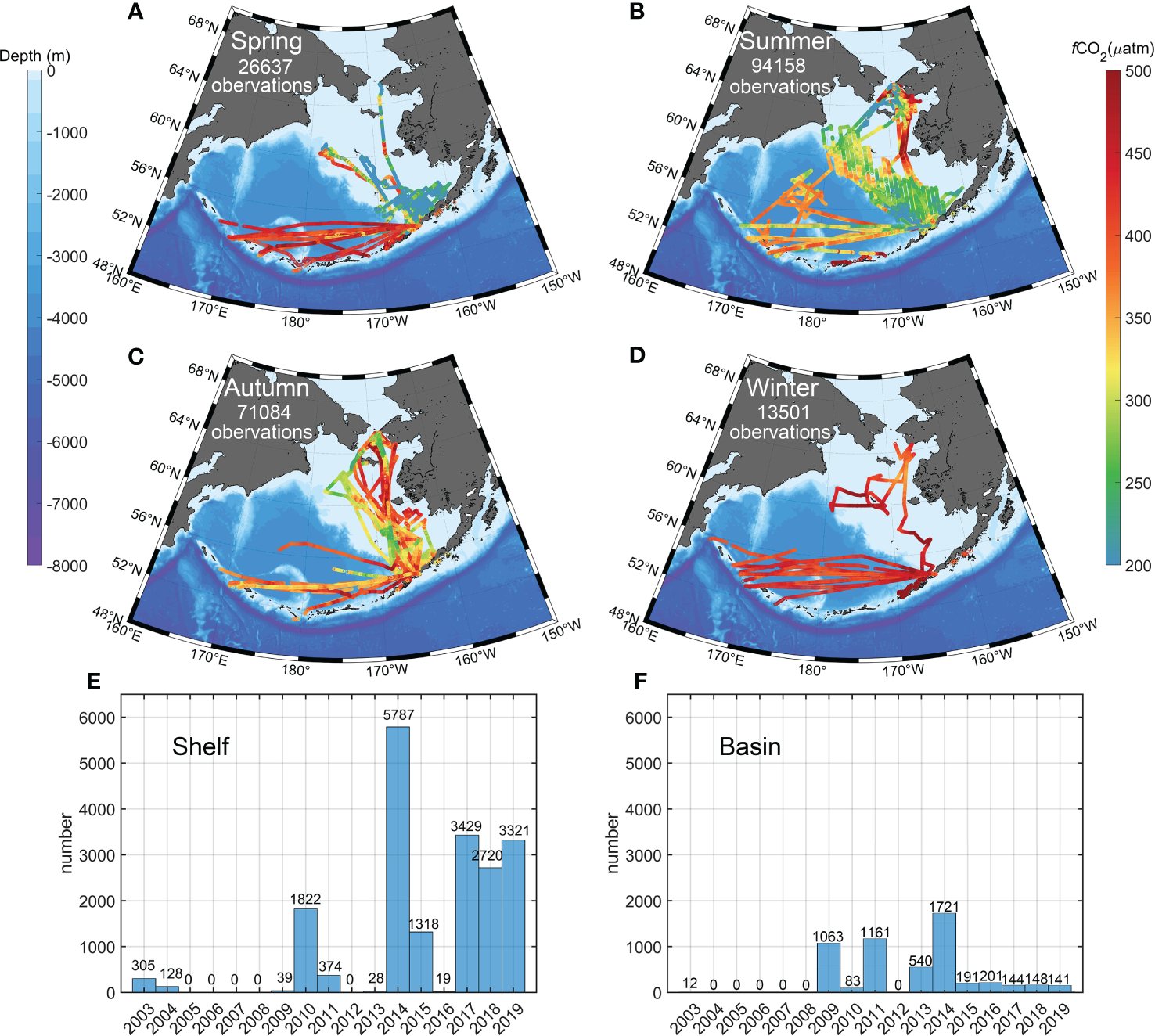
Spatial distribution of SOCAT data in the Bering Sea during 2003 to 2019 in different seasons: (A) March to May, (B) June to August, (C) September to November, and (D) December to February. The measured year of SOCAT data in the Bering Sea from 2003 to 2019 in the (E) shelf and (F) basin.
Following the 4-km grid of the observed data, we matched a variety of environmental parameters to construct matched datasets for training and testing of the retrieved model. Although the spatial and temporal resolutions of these parameters are different, we used the nearest neighbor interpolation method to adjust the spatial resolution to a standard monthly 4-km resolution grid in this study.
Sea surface temperatures were downloaded from the National Oceanic and Atmospheric Administration (NOAA). We used the 1/4° Daily Optimum Interpolation Sea Surface Temperature (OI-SST), which is a long-term climate data record that incorporates observations from different platforms (satellites, ships, buoys, and Argo floats) into a regular global grid, in this research (available at https://www.ncei.noaa.gov/products/optimum-interpolation-sst) (Reynolds et al., 2007; Banzon et al., 2016; Huang et al., 2021). The associated chlorophyll a (Chla) concentrations were taken from a global 4-km-resolution monthly data product compiled by NASA’s MODIS Ocean Science Team (Nasa Goddard Space Flight Cente, 2014), which was calculated using an empirical relationship derived from in situ measurements of Chla and blue-to-green band ratios of in situ remote-sensing reflectance (Carder et al., 2004). The sea surface height (SSH) and mixed-layer depth (MLD) were extracted monthly from the Global Ocean Physics Reanalysis Glorys12V1 (PHYS 001-030) products at a resolution of 1/12° (~8 km) from the Copernicus Marine Environment Monitoring Service (CMEMS) (https://doi.org/10.48670/moi-00021). We extracted the dry air mole fractions of CO2 (xCO2) from CarbonTracker (version 2019B; https://doi.org/10.25925/20201008), which is a modeling system developed by NOAA that provides global estimates of surface atmosphere fluxes and four-dimensional CO2 data (Jacobson et al., 2020). The bathymetry was extracted from the global ETOPO1 database (from NOAA, 2022) (Amante and Eakins, 2009). The list of all products used in the calculations is summarized in Table 1.
Table 1
| Predictor | Dataset | Resolution | Reference |
|---|---|---|---|
| SST | OISST | 0.25°, daily | Huang et al. (2021) |
| Chla | MODIS | 0.0417°, monthly | Carder et al. (2004) |
| MLD | CMEMS | 0.083°, daily | |
| SSH | CMEMS | 0.083°, daily | |
| xCO2 | CarbonTracker | 3° × 2°, daily | Jacobson et al. (2020) |
| Bathymetry | ETOPO1 | 0.017° | Amante et al. (2009) |
Environmental dataset used for pCO2 retrieval.
In the process of calculating the flux, we added extra parameters to estimate the air–sea CO2 flux, including sea surface 10-m wind and atmospheric pressure. Sea surface 10-m wind data were from the cross-calibrated multiplatform (CCMP) vector wind analysis dataset Mears et al., 2022, which combines satellite measurements, in situ measurements, and a background wind field into complete maps of ocean winds every 6 h with biases lower (by almost 0.5 m/s) than those of buoys (Mears et al., 2019). We also compared many satellite and reanalysis wind speed products and finally chose the CCMP wind speed product due to its suitable temporal coverage and accurate characterization. Atmospheric pressure data were from the European Centre for Medium-Range Weather Forecasts Reanalysis v5 reanalysis (ERA5) dataset, which embodies a detailed record of the global atmosphere, land surface, and ocean waves from 1950 onward, providing an hourly output throughout with 37 pressure levels (Hersbach et al., 2020). We used the sea surface pressure from a 0.25° square latitude–longitude grid. The sea ice concentration (SIC) data were obtained from the National Snow and Ice Data Center (NSIDC) Climate Data Record at a spatial resolution of 25 km and a monthly temporal resolution (Meier et al., 2013).
2.3 Air–sea CO2 flux calculation and algorithm performance index
The global air–sea CO2 flux is often estimated by a bulk method in which in situ pCO2 measurements in seawater are combined with a wind-speed-dependent gas transfer velocity (Weiss, 1974b; Wanninkhof, 2014):
where (mol m−2 yr−1) is the air–sea CO2 flux; is the gas transfer velocity; is the solubility of CO2 in seawater (mol m−3 µatm−1); (µatm) and (µatm) are the partial pressure of surface ocean CO2 and atmospheric CO2, respectively, in the marine boundary layer; is the sea ice concentration of ocean area covered by sea ice; is the wind speed 10 m above sea level; and denotes the Schmidt number calculated from SST and sea surface salinity (SSS). We used SIC in this study because sea ice, an imperfect barrier to gas exchange, has an important effect on air-sea CO2 flux (Long et al., 2011; Loose et al., 2014; Butterworth and Miller, 2016). However, whether the effect of sea ice on gas exchange is nonlinear (Loose et al., 2009; Loose et al., 2014) or linear (Butterworth and Miller, 2016; Prytherch et al., 2017) is still under debate, and for simplicity, only linear ice corrections were used in this work. In addition, we used 99% when the SIC was greater than 99% to allow for air-sea CO2 exchange through fracture, lead, and brine channels (Semiletov et al., 2004). All data used here can be sourced in Section 2.2. The sink–source pattern of CO2 flux was determined by the difference between ocean pCO2 and atmospheric pCO2 (ΔpCO2); that is, a positive value of ΔpCO2 corresponds to a CO2 source, while a negative value corresponds to a CO2 sink.
The carbon sink in a total area is usually conducted by the area integral of air-sea CO2 flux. In the Bering Sea, we summed the results of multiplying each grid flux by the area of each grid of three parts (the basin, the shelf and the area of the Aleutian Islands coast). The net CO2 flux in a subregion was estimated by multiplying the mean CO2 flux density among the available pixels and normalizing to the total area. In addition, the high-latitude pCO2 is missing due to the unavailable Chla. In the processing of ocean color satellite data, atmospheric correction usually fails under high solar zenith angles with weak sunlight signals, which usually occurs in winter in high-latitude areas. Therefore, there are large blank areas of missing Chla and corresponding reconstructed pCO2 and flux in Jan. and Dec. To reduce the effect of this vacancy on the area integral of air-sea CO2 flux estimation, we used the seasonal average, which is calculated through adjacent months at the same location, to replace the vacancy.
The root-mean-square error (RMSE) and correlation coefficient (R2) were used as the standard statistical metrics to measure model performance in this study. The RMSE was calculated for the dataset as follows:
where is the index of the samples, are the observation measurements, and are estimates from the model.
2.4 Seasonal difference calculation of pCO2
The seasonal difference calculation of pCO2 was calculated by using the following four steps. First, a third-order polynomial (to account for trends) and fourth-order harmonic function (to reproduce the seasonality) were fitted to all grid data to reproduce the full seasonal cycle (Graven et al., 2013).
where is time in years and is the period, chosen here as 1 yr. Second, we recreate the seasonal cycle of a certain year by fitting equation (4) to every full analysis year, including the year before and after that, to create a three-year running time series. 2003 and 2019 are reconstructed using the two following or preceding years. Third, from the resulting harmonic function f(t) segments, the mean of the months January, February and March was used as the winter average and July, August and September as the summer average. Then, we calculated winter minus summer for a certain year as the seasonal difference. Finally, the trends in these seasonal differences are calculated from the slope of the linear regression line fit to the 17-year time series.
3 pCO2 algorithm and validation
3.1 Machine learning algorithms
Based on the large match-up dataset, we tried various machine learning methods, including support vector machine, eXtreme gradient boosting, Gaussian-process-based kernel machine learning approach (GPR), and random forest. Among them, the GPR method was found to have optimal results in the retrieval of pCO2 in the Bering Sea (the comparison of algorithm performance can be found in the Table 2).
Table 2
| Training | Testing | |||||
|---|---|---|---|---|---|---|
| RMSE | r2 | MAE | RMSE | r2 | MAE | |
| (μatm) | (μatm) | (μatm) | (μatm) | |||
| Random forest | 29.25 | 0.87 | 16.28 | 26.65 | 0.88 | 10.17 |
| Support vector machine | 44.86 | 0.69 | 28.93 | 44.51 | 0.61 | 24.45 |
| Neural network | 39.68 | 0.76 | 29.05 | 39.21 | 0.69 | 32.9 |
| Multiple linear regression | 60.51 | 0.43 | 47.78 | 59.51 | 0.35 | 56.44 |
| e-Xtreme gradient boosting | 42.09 | 0.74 | 31.98 | 44.59 | 0.71 | 30.42 |
| Gaussian process regression (GPR) | 19.18 | 0.93 | 14.86 | 21.82 | 0.91 | 10.04 |
Comparison of algorithm performance of various machine learning methods.
Bold indicates the algorithms used in this study.
The GPR approach allows handling the model selection issue within a Bayesian framework in a completely automatic way, thus offering the potential advantage of avoiding the traditional empirical and tricky tuning of the free parameters of the model (Pasolli et al., 2010). GPRs are usually highly flexible and accurate for prediction over new inputs closer to training data points, and recent studies have demonstrated the effectiveness of GPR for time-series gap-filling applications (Mateo-Sanchis et al., 2018; Pipia et al., 2019; Belda et al., 2020). Furthermore, GPR has exhibited robust performance in some sea surface biophysical retrieval approaches and therefore has outperformed other machine learning regression algorithms, such as random forest and artificial neural networks, especially in retrieving biophysical parameters from satellite data (Verrelst et al., 2012; Verrelst et al., 2015; Rivera-Caicedo et al., 2017). Pipia et al. (2021) proposed a GPR-based gap-filling strategy and generation of multi-orbit cloud-free green leaf area index maps with an unprecedented level of detail. Svendsen et al. (2020) used a Gaussian process to estimate the chlorophyll content, colored dissolved matter, and inorganic suspended matter from multispectral data acquired by the Sentinel-3 OLCI sensor. Blix et al. (2018) used the GPR machine learning model to estimate the complex waters against in situ measurements over Lake Balaton in 2017 based on the Ocean and Land Color Instrument (OLCI) onboard the Sentinel 3A satellite. The effectiveness of this approach in the context of estimation of biophysical parameters offers a new alternative to state-of-the-art regression methods such as those based on artificial neural networks and support vector machines (Pasolli et al., 2010). Based on the characteristics of the Bering Sea and the previous research, we inferred that the strengths of GPR on biophysical environmental parameters (Verrelst et al., 2012; Verrelst et al., 2015; Rivera-Caicedo et al., 2017) and the advantages in learning from small samples (Ly et al., 2021) can help the algorithm to reconstruct sea surface pCO2 well in the Bering Sea. Thus, we chose to use the GPR method to retrieve pCO2 in the Bering Sea.
3.2 GPR method for pCO2 in the Bering Sea
We used time and location data from in situ pCO2 measurements to identify a set of pCO2 values with matched environmental parameters. These gridded monthly standard products were used in the pCO2 model development. The predictor variables of the model were a set of environmental parameters associated with the Bering Sea carbonate system based on some previous studies (Song et al., 2016; Chau et al., 2022), including SST, Chla, MLD, SSH, xCO2, and bathymetry.
In many other studies, these parameters represent physical, chemical, and biological proxies determining the distribution of sea surface pCO2. Here, both SST and MLD were used in the model to account for the influence of thermodynamic and DIC variation in pCO2 (Landschützer et al., 2013). Meanwhile, Chla is commonly used as a “tuning” parameter to emphasize biological activity and primary productivity (Chen and Hu, 2017). SSH, however, was used to characterize the horizontal current flows and to capture the mixing and convergence of water masses at the ocean surface (Chau et al., 2022). In addition, bathymetry was collected to identify the two different carbonate systems: the ocean basin and the shelf.
We tried to incorporate sea surface salinity into the input data. Due to the large uncertainty of various salinity datasets in the Bering Sea, the input data produced low-quality results, so we removed the salinity parameter. The SSH usually contains contributions from high- and low-frequency changes in steric (temperature and salinity) signals and ocean circulation (Meyssignac and Cazenave, 2012; Zhou et al., 2012; Volkov et al., 2022). Here, we used SSH to relatively optimize the performance of our algorithm in the lack of high-quality salinity data. Remote sensing reflectance has been used as input in other studies; however, in the Bering Sea, the model performance with remote-sensing reflectance as inputs was not satisfactory and may form a redundancy of input quantities similar to chlorophyll, as chlorophyll products are usually retrieved from remotely sensed reflectance data. Thus, after trying various combinations, we finally chose six independent environmental predictors: SST, SSH, MLD, Chla, xCO2, and bathymetry in the pCO2 model development; details of the datasets are given in Section 2.2.
3.3 Model training and validation
We divided the underway pCO2 match-up dataset into three parts. First, to ensure the final independent validation, we selected data from the two longest cruises: One was from a cruise in the Bering Basin in October 2009, and the other was from a cruise in the continental shelf sea in July and August 2019 (Figure 3A). These are the longest cruises in each of the two regions to ensure the enough data number and spatial coverage, and we used them as a third completely independent data to validate the algorithm performance, beyond the training dataset and testing data. These cruise-based observations were used for an extra-validation, which put a higher demand on the robustness of the algorithm. To verify that the two cruises are not special, we randomly chose random sets of cruises covering the basin and shelf for independent validation and developed a model with the same parameters and methods. The accuracy of the four models is very close to that of the original model, demonstrating that our modeling is stable with changes in the independent validation (four cases of the model validation results from different random selections of independent cruises can be found in the Supplemental Material).
Figure 3

Location sites of the (A) independent validation dataset, (B) training dataset, and (C) testing dataset. The validation dataset includes two independent cruises measured in October 2009 in the basin and in July and August 2019 over the continental shelf. Comparison of training pCO2 in the (D) basin and (E) continental shelf with the observations. Comparison of testing pCO2 in the (F) basin and (G) continental shelf with the observations. Colors indicate the amount of data within each grid, and red lines are one-by-one lines.
Then, we derived a relationship between the pCO2 field and environmental predictors based on a GPR method, with 75% of the remaining gridded pCO2 (produced from SOCAT v2022 cruise data, see more details in Section 2.2) used as the training dataset and 25% as the model testing dataset (Figures 3B, C). We therefore could establish nonlinear relationships between six independent environmental predictors (SST, SSH, MLD, Chla, xCO2, and bathymetry) and pCO2. The reconstructed pCO2 field matches the SOCAT data well. In both the basin and continental shelf, a high agreement between the training pCO2 and the gridded SOCAT v2022 data is demonstrated, with an overall mean R2 of 0.93 and RMSE ~ 19.18 µatm (based on 16,985 observations) (Figures 3D, E). This good fit can also be found in the testing, with an RMSE = 12.56 μatm in the basin and 23.08 μatm in the shelf (Figures 3F, G).
In independent validation, we obtained a mean R2 of 0.94 and RMSE ~ 23.49 µatm (based on 1424 observations) (Figure 4). Although there are some errors in regions of extreme gradient variations, we were still able to capture the correct trends in these rapidly changing regions (Figures 4A, B). The validation indicated that the GPR method can accurately reconstruct pCO2 in the Bering Sea (Figure 4C). However, because of the lack of in situ measurements, our estimates along the western coast of the Bering Sea (e.g., the Gulf of Anadyr) are tentative extrapolations without sufficient validation. We note that there is no in situ data in the self of the Bering Sea during 2005-2008 and no data available in the basin before 2008, and these data gap may induce the uncertainty of time series analysis. We try to develop satellite retrieval algorithm and to reconstruct the satellite-based pCO2 from 2003 to 2019, but we will also emphasis such uncertainty and discuss the time series from 2009 to 2019.
Figure 4

Comparison of reconstructed pCO2 with two independent validation cruise datasets over (A) the basin and (B) the continental shelf. (C) Comparison of validation pCO2 in the Bering Sea with the observations.
4 Results
4.1 Seasonal variation in pCO2 and air–sea CO2 flux
Based on a novel GPR method with multisource remote-sensing data, we generated monthly 1/24° (~4 km) resolution pCO2 and reconstructed the air–sea CO2 flux during the period from January 2003 to December 2019. The 17-year climatological monthly pCO2 data exhibit marked seasonal and spatial variation (ranging from 250–450 µatm) in the Bering Sea (Figure 5). In the Bering Sea basin, sea surface pCO2 decreases continuously from April to July and reaches its annual minimum (326.2 μatm) in August and rises from September to November, eventually reaching a peak (441.2 μatm) in December; a similar pattern can be found in the shelf area where sea surface pCO2 reaches its annual minimum (291.6 μatm) in May with a peak (416.3 μatm) in January. Although both the continental shelf and the ocean basin exhibit typical subpolar pCO2 seasonal patterns, with low pCO2 in summer and high pCO2 in winter and spring, the pCO2 in the shelf region declines 2–3 months earlier than that in the ocean basin area and remains at lower values for longer periods. Our reconstructed dataset reconstructs the large summer gradient in pCO2 between the basin and shelf well (Figure 5), and this phenomenon is also confirmed by the measured data (Figure 2). The coastal region of Alaska has experienced extremely high pCO2 in the summer. The seasonal amplitude of seawater pCO2 is almost a factor of 3–4 greater than that of the atmospheric pCO2 (Figure 6A).
Figure 5
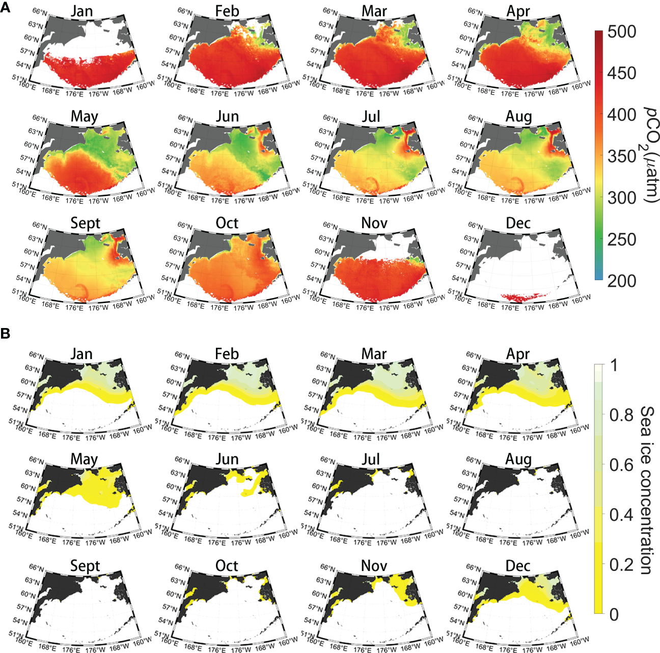
(A) Climatological monthly sea surface pCO2 in the Bering Sea during 2003-2019. (B) Climatological monthly mean sea ice concentrations (SICs) in the Bering Sea during 2003-2019.
Figure 6
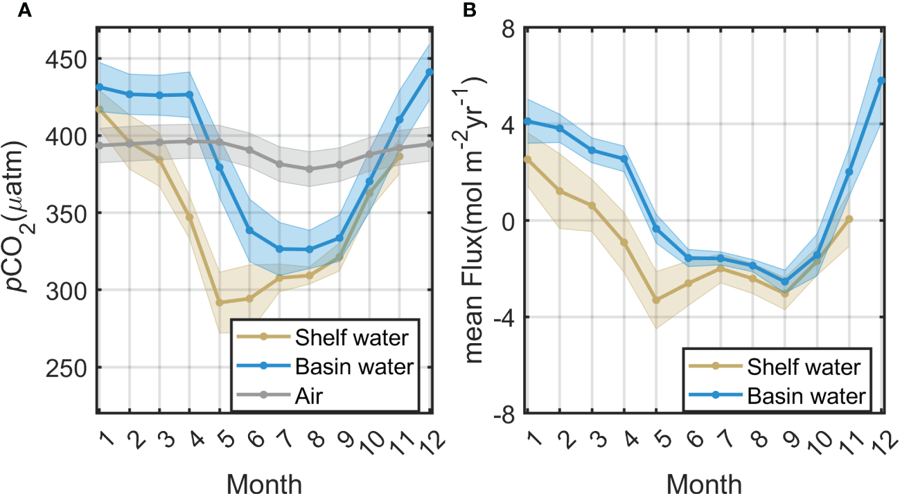
Mean seasonal variability in (A)pCO2 and (B) air–sea CO2 flux in the Bering Sea basin and shelf from 2003 to 2019. Shadows of the curve represent the statistical standard deviation.
Based on the satellite-derived pCO2, sea surface wind speed, xCO2, and SST, we estimated the long-time-series air–sea CO2 flux in the Bering Sea from 2003 to 2019. The seasonal variation in air–sea CO2 fluxes in the Bering Sea is closely related to the seawater pCO2 pattern, with a mean air-sea CO2 flux of approximately ± 0.7 mol m−2 mon−1 (Figure 7). The Bering Sea basin exhibits dramatic seasonal amplitudes, with sea water releasing CO2 to the atmosphere from November to April and becoming a sink during June to October (Figure 6B). The continental shelf, however, continues to behave as a sink for the atmosphere and reaches its maximum absorption in spring (Figure 6B), except along the Alaskan coast, which exhibits a weak source in summer, especially from June to August. In addition, seawater in the southern Bering Sea (coastal Aleutian Islands) is a total source to the atmosphere, with the strongest emission occurring in spring. As mentioned in Section 2.3, remote-sensing reflectance data and Chla products under high solar zenith angles are usually invalid in winter in high-latitude areas. Therefore, there are large blank areas of missing Chla and corresponding reconstructed pCO2 and flux in Jan. and Dec. in Figures 5, 6, which would lead to uncertainty in the estimation.
Figure 7
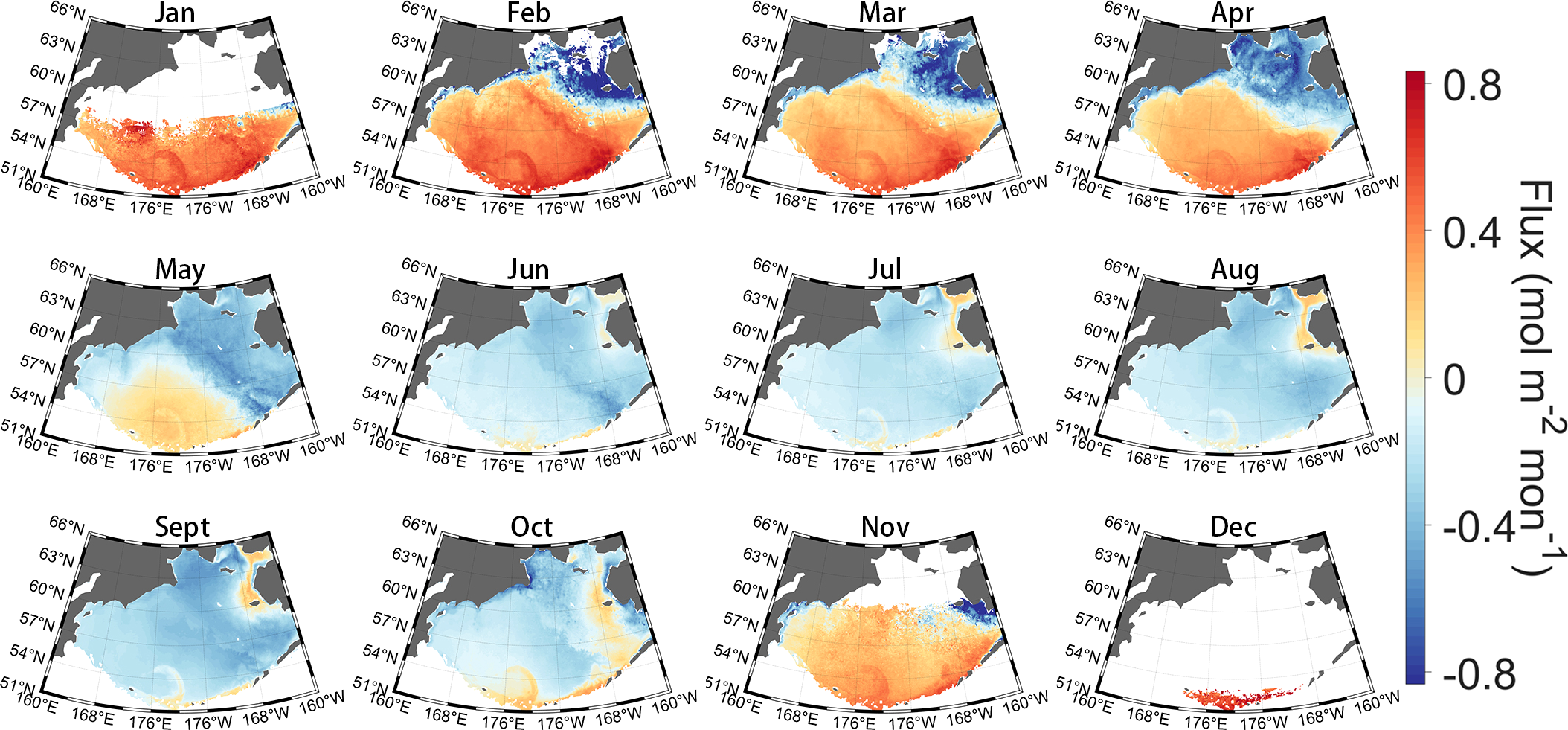
Climatological monthly air–sea CO2 flux in the Bering Sea during 2003-2019. That flux calculation is related to the sea ice concentration (SIC) (Eq. 1); please see Figure 5B for the climatological monthly mean SIC.
4.2 Long-time-series variation in air–sea CO2 flux
We averaged the valid pCO2 data for each month and then calculated the annual average based on the monthly average results. From 2003 to 2019, atmospheric pCO2 in the Bering Sea increased steadily (2.13 ± 0.09 μatm yr−1, P< 0.01). Meanwhile, sea surface pCO2 in the basin area increased more rapidly than that in the atmosphere (2.82 ± 0.63 μatm yr−1 in 2003-2019 and 2.95 ± 0.57 μatm yr−1 in 2009-2019, P< 0.01). However, there is no clear trend on the continental shelf, where sea surface pCO2 fluctuates in the range of 347 ± 12 μatm, consistently maintaining a low value of<360 μatm with seasonal fluctuations of ±63 μatm (Figure 8A). As a result, the trend of the annual mean air–sea pCO2 difference (ΔpCO2) in the basin area rises at a slow rate, while it declines rapidly in the shelf area. Small variations occurred in ΔpCO2 during 2003-2008, which might contain some uncertainty as the in-situ data are unavailable during this period. During 2009-2019, the decreasing rate of ΔpCO2 (4.37 μatm yr-1) in the shelf is approximately three times that of the increasing rate in the basin; against the background of continuously increasing atmospheric CO2, sea surface pCO2 exhibited insignificant changes in continental shelf, which also exacerbated the air-sea ΔpCO2 (Figure 8C). Thus, the Bering Sea basin was a slowly developing CO2 source, while the carbon sink in the Bering Sea shelf area has been increasing significantly. Meanwhile, the annual mean wind speed in the Bering Sea changed little during the study period, and the mean wind speed in the sea basin was always 1 m s−1 greater than that on the shelf (Figure 8B). Note that in 2008-2019, the mean wind speed exhibited a slight increasing trend: 0.052 m s-1 yr-1 (shelf, P = 0.013) and 0.043 m s-1 yr-1 (basin, P = 0.038). Then, we analyzed the annual variation of sea surface pCO2 and atmospheric pCO2 in each month to check if the trends are various in season (Figures 8D, E). During 2003-2019, the atmospheric pCO2 increased at a similar rate (2.19 ± 0.02 μatm yr-1) in all months (Figure 8B), while sea surface pCO2 exhibited different trends in different months. In general, except April-June, the growth rates of sea surface pCO2 were around 1.63 ± 0.98 μatm yr-1, p-value< 0.05). However, the growth rates were not significant in April-June (p-value > 0.05), indicating that sea surface pCO2 fluctuated within a certain range without significant annual trends in these months. This may be due to the strong photosynthesis and high primary productivity during May to August and the biological effects facilitate the carbonate buffering system to some extent. When weakened productivity and deep DIC upwelling occur simultaneously, large growth rates occurred in October (2.6 μatm yr-1) and November (2.5 μatm yr-1), which even higher than the atmospheric growth rate (Figure 8F).
Figure 8
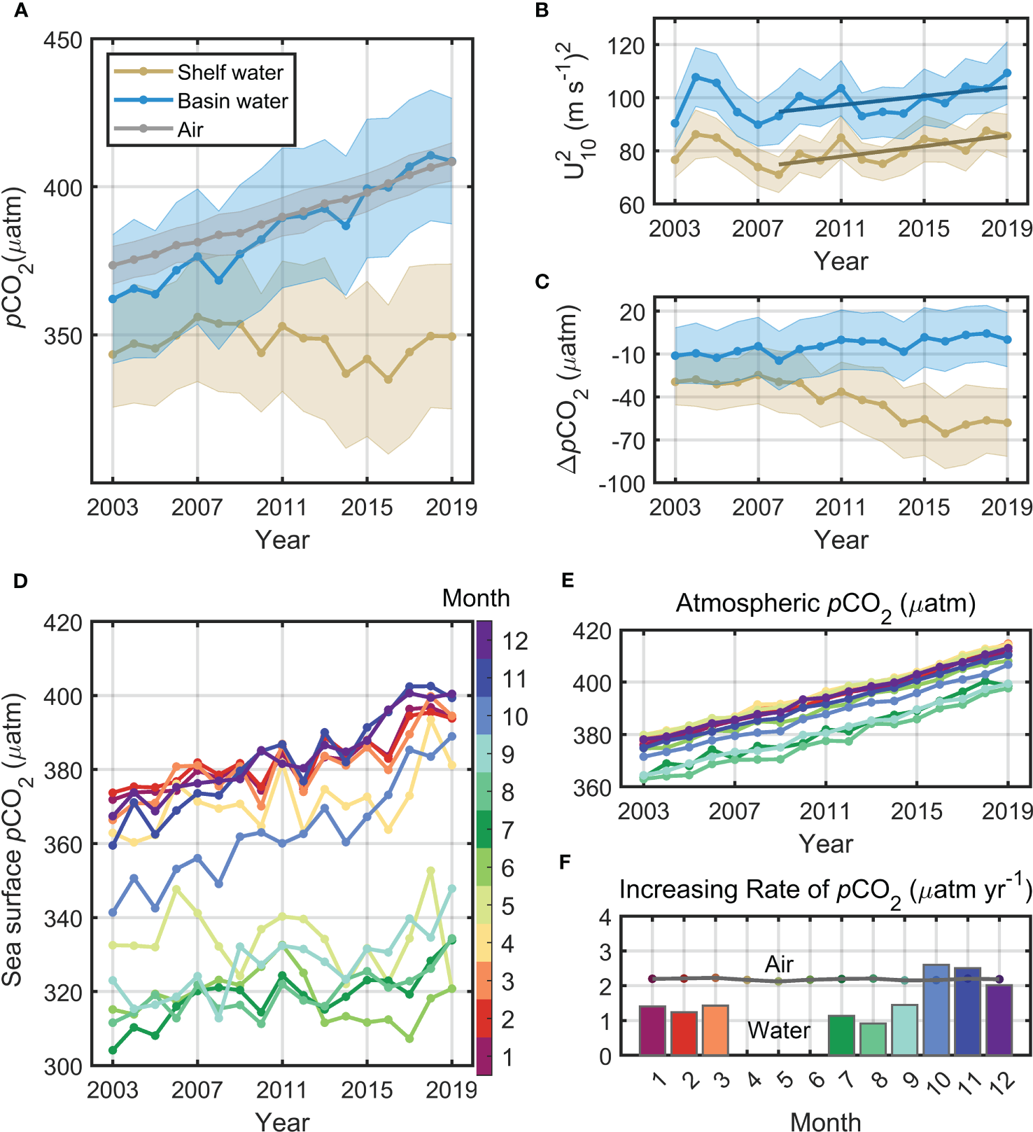
Time series of annual (A)pCO2, (B) square of the 10-m wind speed on the sea surface , and (C) air–sea pCO2 difference (ΔpCO2) over the basin and shelf from 2003 to 2019. The dark lines in (B) are the regression lines during 2008-2019. Shadows of the curve represent the statistical standard deviation. Time series of the annual variation of (D) sea surface pCO2, (E) atmospheric pCO2 and (F) growth rates. In Figure F, bars are growth rates for sea water and polylines for atmosphere in specific months from 2003 to 2019, and the growth rate of sea surface pCO2 in Apr. to Jun. was not shown, because they failed in the significance tests (p-value > 0.05). Figs D, E and F share the same color bar which indicate the months.
We estimated the annual absorption of the sea basin, continental shelf, and whole Bering Sea (Figure 9) with the area integral of the air-sea CO2 flux. Note here that the total CO2 uptake does not exactly match the trend of the mean air–sea CO2 flux because CO2 uptake is the integral of the gridded flux with respect to the gridded area. Consequently, southern grids will produce greater CO2 uptake or release than those in the north under the same carbon flux. As a result, the whole Bering Sea exhibited an increasing carbon sink with an integral increase in air-sea CO2 fluxes from 6 to 19 TgC over 17 years. The variation of total air-sea carbon flux was insignificant in 2003-2008, and consistently increased from 2011 to 2015, maintaining at 15-19 TgC since 2015. However, due to the insufficient observations for the continental shelf in 2003-2009, we cannot confirm whether the GPR algorithm underestimates air-sea CO2 sink, which may have contributed to the rapid increase in 2011-2015. Although the Bering Sea is generally characterized as an important carbon sink with an average air–sea CO2 flux of 8.87 TgC yr−1, this absorption is almost entirely driven by the on-shelf regions and the green belt. The deep basin, in contrast, is a high-nutrient, low-chlorophyll region with increasing sea surface pCO2 and acts as a CO2 source with increasing CO2 emissions during the study time period. The upwelling along the coastal Aleutian Islands contributed to the regional high pCO2 (Kelley and Hood, 1973; Sapozhnikov et al., 2011), whereas this upwelling-induced CO2 emission did not exhibit a significant trend over the study period from 2003 to 2019. The increased wind speed from 2008-2019 also contributed to a larger air–sea CO2 flux. In conclusion, the carbonate systems in the basin and continental shelf of the Bering Sea evolved in different directions under the background of the continuous rise in atmospheric pCO2.
Figure 9
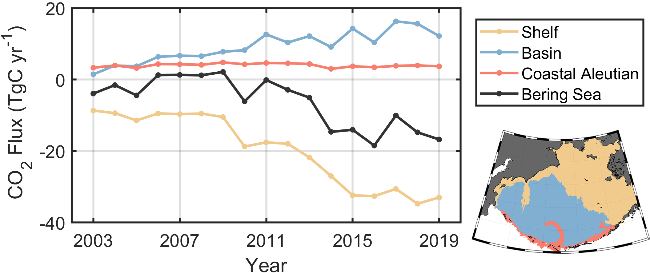
Time series of the annual mean air–sea CO2 flux sink in different subregions of the Bering Sea from 2003 to 2019. The lower right panel is a schematic representation of the subregions; the zoning is based on the 200-m isobath.
5 Discussion
5.1 Seasonal pCO2 control mechanisms
To explore the drivers of air–sea CO2 fluxes in the Bering Sea, we used a method similar to that developed by Takahashi et al. (2002) and calculated the effects of temperature (T) and all other non-temperature processes (nonT) on the sea surface pCO2 differences. We used temperature-normalized pCO2 to remove the temperature control; this can be expressed as follows:
where the quantity is the temperature-normalized pCO2; is the sea surface temperature; and is the climatological annual mean calculated from the optimum interpolation sea surface temperature during 2003–2019, as (∂ln pCO2/∂T) is +4.23% °C−1 (Takahashi et al., 1993). Therefore, the effects of temperature (T) and all other non-temperature processes on the sea surface pCO2 differences can be estimated as follows:
where represents the impact of temperature (temperature effect) and weights the impact of all other processes, such as the biological effect, upwelling and other mixing processes. is atmospheric pCO2. The sum of temperature and non-temperature pCO2 components is equal to the seasonal variability at any given time under the assumption that the annual mean pCO2 should be well represented (Takahashi et al., 2002; Cross et al., 2014). Because we aim at the mechanisms affecting seasonal air-sea CO2 fluxes, the atmospheric pCO2 was selected as a reference when calculating (Wang et al., 2022). Hence, the sum of and is equal to ΔpCO2(= ) at any given time in this study.
Based on Eqs. (5) and (6), we estimated the effects of temperature and non-temperature effects in the Bering Sea from pCO2 data estimated from satellite data. Figure 10 shows that the spatial distributions of and differ. Bates et al. (2011) indicated that the biological effect, that is, the balance of photosynthesis and respiration, is the most dominant process driving variability in non-temperature processes on the continental shelf in the Bering Sea. Our findings also suggested that non-temperature effects, including biological contributions, upwelling and seasonal mixing, together dominate the surface pCO2. As and . have opposite effects, and the non-temperature effect is a factor of ~2–4 greater than the temperature effect. The mean temperature effect of pCO2 is 12.7 μatm, whereas the mean non-temperature effect is −51.8 μatm. This difference is consistent with the previous conclusion that temperature is not the primary control mechanism in the Bering Sea (Takahashi et al., 2002; Song et al., 2016). In addition, the effect of temperature on pCO2 is positive, and the strongest temperature effects occur within the Norton Sound (>40 μatm) (Figure 10A). In contrast, the effect of the non-temperature component is negative and more widespread, with thmost impacted area being in the Gulf of Anadyr (<-100 μatm) (Figure 10B).
Figure 10
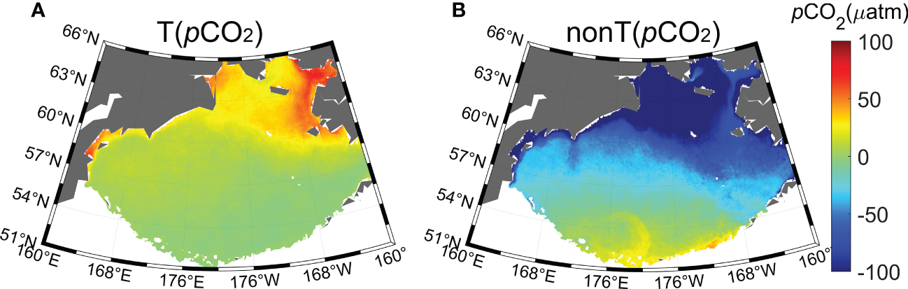
Climatological distribution of (A) temperature effect and (B) non- temperature effect in the Bering Sea.
5.2 Water mass variation and the influence on pCO2
To analyze the pCO2 distributions in more detail, we classified water masses in the Bering Sea with respect to the subregions (see Figure 1A). Based on the previous method of water mass classification in the Bering Sea, we discuss the characteristics of six water masses in the Bering Sea: basin winter water (BWW), basin summer water (BSW), shelf winter water (SWW), shelf summer water (SSW), melt water (MW), and Alaskan coastal water (ACW) (Schumacher et al., 1979; Coachman, 1986; Clement et al., 2005; Jinping et al., 2006; Danielson et al., 2017; Lin et al., 2019; Yamashita et al., 2019; Abe et al., 2021; Hirawake et al., 2021; Wang et al., 2022). The classified boundaries of temperature and salinity are given in Table 3. The Bering Sea basin and shelf water bodies can be distinguished from summer and winter by a boundary of 4°C. Salinity can be used to distinguish among the sea basin, shelf, and coast. Low-salinity water near the coast has two sources: melt ice and riverine input, which can be distinguished by temperature. Due to the mixing of MW and ACW, we classified the mixing water masses as either MW or ACW according to their temperature. Due to the lack of cruise data in the nearshore area, we cannot distinguish the mixing of MW with river water. During thermodynamic dominance, pCO2 increases with higher temperature. However, in subpolar regions, pCO2 increases in winter when the seasonal mixed-layer depth is deepening, with DIC-rich water from deep upwelling to the sea surface (Sarmiento, 2013; Fay and Mckinley, 2017; Gallego et al., 2018). In addition, the vertical mixing of high-DIC subsurface waters results in sea surface pCO2 increasing. We also found that the pCO2 in the basin was significantly higher in winter (BWW) than in summer (BSW), suggesting that the Bering Sea basin is not a region of dominant temperature effect on pCO2 (Figure 11). Similar seasonal variations occurred in the shelf and basin with lower pCO2 in summer water than in winter water (Figures 11C, F). Meanwhile, this seasonal difference is more significant in the shelf, which may be because phytoplankton production is higher in the shelf area than in the high-nutrient low-chlorophyll basin. The pCO2 coastal region of Alaska is much more strongly influenced by the low-salinity MW and ACW; however, different types of changes are generated. The MW diluted the seawater, resulting in a lower pCO2 (Figure 11C). In the river plume area, pCO2 is often at a low level because of the photosynthesis of phytoplankton. However, the estuarine areas and nearshore areas are also affected by a large amount of riverine humic and other organic matter from the catchment basin, and strong respiration, mineralization and degradation processes lead to high pCO2 in rivers and estuarine areas. Nishimura et al. (2012) observed high concentrations of dissolved Fe and humic-type fluorescence intensity in a nearly peak river water discharge period in the northern Bering Sea shelf (Yukon River estuary region and St. Lawrence Island polynya region). Strong mineralization and degradation of high concentrations of terrestrial organic matter will lead to high pCO2 in estuaries and offshore areas. Murata (2006) also indicated that coccolithophorid Emiliania huxleyi blooms occurred in coastal Alaska simultaneously in summer with CO2 changes (increase in CO2). During the growth of coccoliths when the calcium carbonate shell is formed, CO2 is released at the same time, resulting in an increase in sea water pCO2. It is different from diatom blooms with CO2 drawdown (Murata, 2006).
Table 3
| Water masses | Salinity | Temperature | |
|---|---|---|---|
| Basin winter water | BWW | >32.5 | >0, ≤ 4 |
| Basin summer water | BSW | >32.5 | >4 |
| Shelf winter water | SWW | >30.5, ≤ 32.5 | >0, ≤ 4 |
| Shelf summer water | SSW | >30.5, ≤ 32.5 | >4 |
| Melted water | MW | ≤ 30.5 | ≤ 0 |
| Alaskan coastal water | ACW | ≤ 30.5 | >0 |
Primary water masses in the Bering Sea.
Figure 11

Carbonate chemistry characteristics of the water mass in the Bering Sea, showing T/S characteristics (A, D), location of the water masses (B, E), and pCO2(C, F). In the T/S diagrams, the dashed line is the freezing line. Water mass designations follow those of Table 3: BWW = basin winter water, BSW = basin summer water, SWW = shelf winter water, SSW = shelf summer water, MW = melted water and ACW = Alaskan coastal water.
We also calculated the temperature and non-temperature effects on pCO2 in each of the six typical water masses (Figure 12). The opposite trend between temperature and non-temperature effects is evident in the Bering Sea basin and the continental shelf, with temperature providing positive values and negative values from non-temperature effects in summer and vice versa in winter. However, regardless of the seasonal change, the non-temperature effect always outweighs the temperature effect, becoming the most dominant control mechanism in the Bering Sea, which can usually be considered a result of seasonal variations in DIC (Takahashi et al., 2009; Gallego et al., 2018). In addition, this non-temperature effect reaches a maximum in the summer over the continental shelf, which may be due to the combined effect of low DIC resulting from the high net community productivity (primary productivity – community respiration) produced and low DIC diluted by high summer river runoff (Mathis et al., 2010; Mathis et al., 2011; Cross et al., 2012).
Figure 12
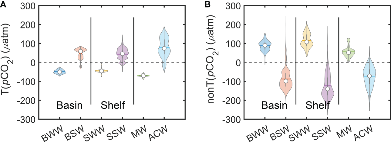
Violin plots of (A) temperature effects T(pCO2) and (B) non-temperature effects nonT(pCO2) of the typical water masses. Note that the width of the violin curve corresponds with the kernel density of the data. Statistical results shape each colored symbol, that is, the inside hollow circles indicate the median, the horizontal lines indicate the mean, and the external shapes indicate the frequency.
5.3 Strengthening of pCO2 seasonal variations
Many studies have found that the amplitude of pCO2 seasonal differences have been increasing substantially in recent decades based on observed data or model-based predictions. Landschützer et al. (2018) indicated that the seasonal differences increase at a rate of 1.5 ± 1.1 μatm per decade observed at the Hydrostation ‘S’/Bermuda Atlantic time-series study site and at the Hawaiian Ocean time-series station, which was 3.8 ± 2.4 μatm per decade. Furthermore, model-based predictions also support the increasing seasonal difference in pCO2 in the South Atlantic, Pacific, and North Atlantic (Doney et al., 2009; Hauck and Völker, 2015; Mcneil and Sasse, 2016).
In the Bering Sea basin, the satellite-derived pCO2 reveals no remarkable change in the seasonal amplitude (1.3 μatm per decade); however, it has been rapidly increasing on the continental shelf from 2003 to 2019, approaching 14 μatm per decade (the calculation method can be found in the supplemental materials). Although a considerable amount of winter data is missing in the shelf of the Bering Sea from our reconstructed pCO2 dataset (which both resulted from the failure of satellite processing at the large zenith angle in high latitudes in winter and the inability to observe water signals due to ice cover), there is some uncertainty in the time-series trend estimation. We regarded that such missing data might be systematic, and the trend estimated from satellite products could be referable, as Landschützer et al. (2018) also showed the average increasing rate at 55°N can be ~8 μatm per decade. In addition, the seasonal cycle in high-latitude areas has a maximum in winter, leading to a positive winter-minus-summer difference in pCO2. Whether in the sea basin or on the shelf, Chla is relatively stable in autumn and winter, while the peak caused by blooms in spring and summer fluctuates (1.5-2.3 μg/L in the continental shelf and 2.5-3.0 μg/L in the basin) with significant interannual variation (Figure 13A). The temperature shows a large seasonal amplitude (Figure 13B). The sea surface height of the basin increases throughout the study time period, while there is no significant trend in the shelf (Figure 13C). In addition, the mixed-layer depth shows the most complex interannual variability, with an abrupt decrease in the mixed-layer depth occurring in the basin (since 2013), while at the same time, the shelf area is increasing with a smaller trend (Figure 13D). Compared to the Bering Sea basin, the greater seasonal amplitude of pCO2 in the continental Bering Sea is mainly the result of decreasing pCO2 in summer (Figure 13E), combined with the stable growth of atmospheric xCO2. The final interannual variation in ΔpCO2 is shown in Figure 13F.
Figure 13
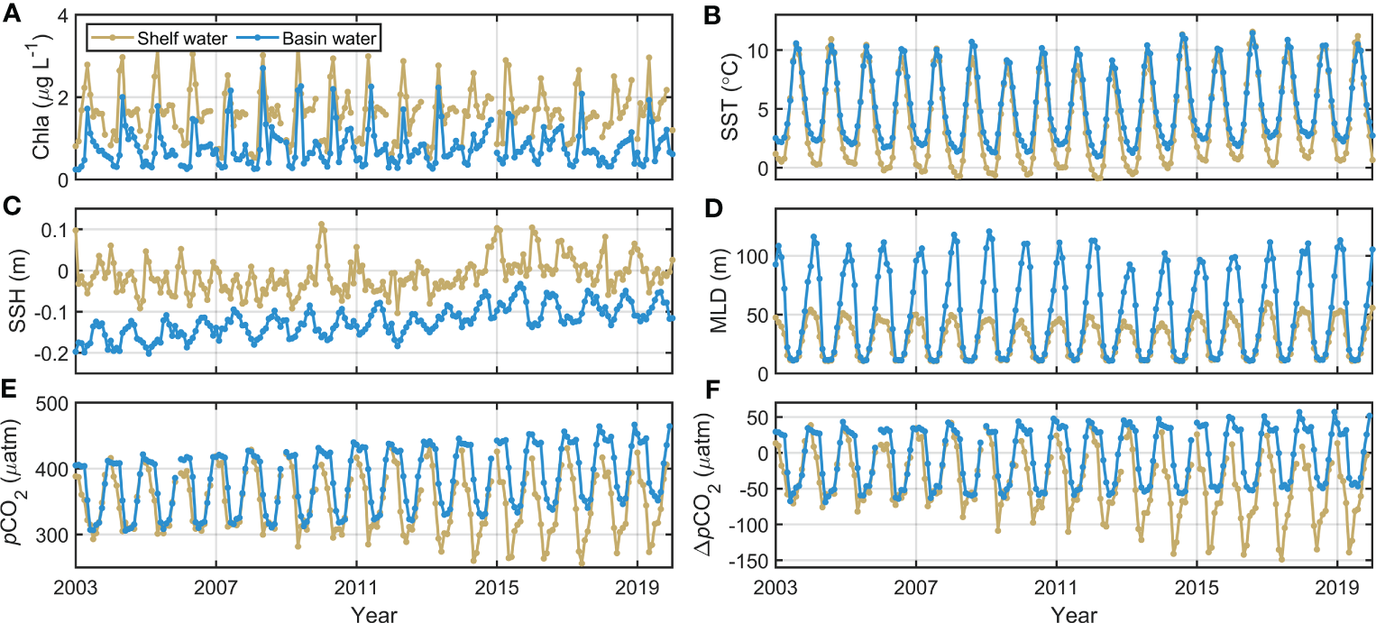
Long-time-series monthly mean Bering Sea (A) Chla, (B) SST, (C) SSH, (D) MLD, (E)pCO2, and (F) ΔpCO2 from 2003 to 2019.
Previous studies have identified two possible mechanisms that may drive the increase in seasonal differences: the long-term increase in the mean concentration of CO2 in the surface ocean and the reaction of the added CO2 with the carbonate ions in seawater (Landschützer et al., 2018). Taking these hypotheses into consideration, we analyzed the mechanisms in the continental Bering Sea. First and foremost, because sea surface pCO2 increases, the pCO2 variation with temperature also increases; thus, even the same seasonal temperature difference can strengthen the seasonal pCO2 amplitude. This effect is more applicable to explain the variation in seasonal amplitude in the basin. The continental Bering Sea remained at 348 ± 12 μatm during 2003–2019, exhibiting an unclear trend. Second, the reaction of the continuously added CO2 with the carbonate ions in continental seawater results in a reduction in the capacity of the surface ocean CO2 system. Hauck et al. (2015) showed that the seasonal drawdown of carbon by biological production contributes an even larger share to the total CO2 uptake as the Revelle factor increases in this century in the Southern Ocean and other regions governed by strong seasonality (Hauck et al., 2015). In other words, the same amount of biological production will lead to stronger CO2 uptake over the course of the century. The strong seasonal decrease in DIC might increase the uptake of CO2 in the Bering Sea. Furthermore, this is particularly vital in systems with strong seasonality, such as at high latitudes, where darkness inhibits biological production in winter. Increased seasonal variability in sea surface pCO2 largely enhances the influence of ocean acidification on marine organisms by exposing them earlier to higher levels of ocean acidification (Doney et al., 2009; Bates et al., 2014; Lauvset et al., 2015). This leads to transitions that cross critical thresholds harmful to marine ecosystems and fisheries, such as hypercapnia and low saturation regarding calcium carbonate (Gruber et al., 2012; Lauvset et al., 2015; Mcneil and Sasse, 2016).
6 Conclusion
Along with increasing atmospheric CO2, the total amount of ocean absorption has also been increasing annually, which impacts the ocean carbon sink and biogeochemical processes. The Bering Sea, a vital passage for North Pacific Ocean water to enter the Arctic, will also be deeply affected.
We developed a sea surface pCO2 model based on the GPR method in the Bering Sea and reconstructed the monthly average pCO2 with high spatial resolution over a long time series during 2003-2019 using a set of SST, SSH, MLD, Chla, xCO2, and bathymetry data as input data. We obtained a mean R2 of 0.94 with an RMSE of ~ 23.49 µatm in the independent validation.
On a background of the continuous rise in atmospheric pCO2 (2.1 μatm yr−1), the carbon sink in the basin and continental shelf of the Bering Sea evolved in different directions. From 2003 to 2019, sea surface pCO2 in the basin area increased rapidly (2.8 μatm yr−1); thus, the CO2 emissions from the basin increased. However, there is no clear trend on the continental shelf, which consistently maintains a low value of<360 μatm (with seasonal fluctuations of ±63 μatm) and is a significant carbon sink in the Bering Sea shelf. This is the first long-time-series estimation of the annual CO2 flux for the whole Bering Sea. The results show that the Bering Sea is generally a rising carbon sink and that the main control mechanism here is not the temperature effect. Additionally, extensive biological activity and high primary productivity occur in the shelf of the Bering Sea, which contribute to the annually increasing uptake of atmospheric pCO2. Hence, the total Bering Sea can be deemed an increasing carbon sink. However, the seasonal amplitude in the shelf is also increasing significantly because of the change in the carbonate system, which may reduce the time required for the Bering Sea shelf to reach its upper limit of absorption, and it is worth considering whether the Bering Sea can continue to consume large amounts of atmospheric CO2 in the future.
Statements
Data availability statement
The raw data supporting the conclusions of this article will be made available by the authors, without undue reservation.
Author contributions
SZ, YB, and DP contributed to the conception and analysis of the study; SZ and XH contributed to manuscript preparation; FG, ZJ, TL, and SY helped perform the data processing and participated in constructive discussions. All authors contributed to the article and approved the submitted version.
Funding
This study was supported by the National Natural Science Foundation of China (# 42176177 and 41825014), the Key R&D Program of Zhejiang (# 2023C03011) and the Zhejiang Provincial Natural Science Foundation of China (# 2017R52001 and LR18D060001).
Acknowledgments
We thank NOAA, NASA, CMEMS, GML, ECMWF, NSIDC, and CCMP for providing valuable datasets, and we also thank SOCAT for collecting and processing the released carbonate products. We thank the SOED/SIO/MNR satellite ground station, satellite data processing and sharing center, and the marine satellite data online analysis platform (SatCO2) for their help with data collection and processing.
Conflict of interest
The authors declare that the research was conducted in the absence of any commercial or financial relationships that could be construed as a potential conflict of interest.
Publisher’s note
All claims expressed in this article are solely those of the authors and do not necessarily represent those of their affiliated organizations, or those of the publisher, the editors and the reviewers. Any product that may be evaluated in this article, or claim that may be made by its manufacturer, is not guaranteed or endorsed by the publisher.
Supplementary material
The Supplementary Material for this article can be found online at: https://www.frontiersin.org/articles/10.3389/fmars.2023.1099916/full#supplementary-material
References
1
Abe H. Nomura D. Hirawake T. (2021). Salinity regime of the northwestern Bering Sea shelf. Prog. In Oceanog.198, 102675. doi: 10.1016/J.Pocean.2021.102675
2
Amante C. Eakins B. W. (2009) Etopo1 arc-minute global relief model: procedures, data sources and analysis. Available at: Https://Www.Ncei.Noaa.Gov/Products/Etopo-Global-Relief-Model.
3
Askren D. R. (1972). Holocene Stratigraphic framework, southern Bering Sea continental shelf (Seattle: University Of Washington).
4
Bakker D. C. Pfeil B. Landa C. S. Metzl N. O'brien K. M. Olsen A. et al . (2016). A multi-decade record of high-quality fco 2 data in version 3 of the surface ocean Co 2 atlas (Socat). Earth Sys. Sci. Data8, 383–413. doi: 10.1594/Pangaea.849770
5
Banzon V. Smith T. M. Chin T. M. Liu C. Hankins W. (2016). A long-term record of blended satellite and In situ Sea-surface temperature for climate monitoring, modeling and environmental studies. Earth Sys. Sci. Data8, 165–176. doi: 10.5194/Essd-8-165-2016
6
Bates N. R. Astor Y. M. Church M. J. Currie K. Dore J. E. González-Dávila M. et al . (2014). A time-series view of changing surface ocean chemistry due to ocean uptake of anthropogenic Co2 and ocean acidification. Oceanography27, 126–141. doi: 10.5670/oceanog.2014.16
7
Bates N. Mathis J. Jeffries M. (2011). Air-Sea Co 2 fluxes on the Bering Sea shelf. Biogeosciences8, 1237–1253. doi: 10.5194/Bg-8-1237-2011
8
Belda S. Pipia L. Morcillo-Pallarés P. Rivera-Caicedo J. P. Amin E. De Grave C. et al . (2020). Datimes: a machine learning time series gui toolbox for gap-filling and vegetation phenology trends detection. Environ. Model. Soft.127, 104666. doi: 10.1016/J.Envsoft.2020.104666
9
Blix K. Pálffy K. R. Tóth V. Eltoft T. (2018). Remote sensing of water quality parameters over lake balaton by using sentinel-3 olci. Water10, 1428. doi: 10.3390/W10101428
10
Butterworth B. J. Miller S. D. (2016). Air-Sea exchange of carbon dioxide in the southern ocean and Antarctic marginal ice zone. Geophys. Res. Lett.43, 7223–7230. doi: 10.1002/2016gl069581
11
Cai W.-J. (2011). Estuarine and coastal ocean carbon paradox: Co2 sinks or sites of terrestrial carbon incineration? Annu. Rev. Of Mar. Sci.3, 123–145. doi: 10.1146/Annurev-Marine-120709-142723
12
Carder K. L. Chen F. Cannizzaro J. Campbell J. Mitchell B. (2004). Performance of the modis semi-analytical ocean color algorithm for chlorophyll-a. Adv. In Space Res.33, 1152–1159. doi: 10.1016/S0273-1177(03)00365-X
13
Chau T. T. T. Gehlen M. Chevallier F. (2022). A seamless ensemble-based reconstruction of surface ocean pco 2 and air–Sea Co 2 fluxes over the global coastal and open oceans. Biogeosciences19, 1087–1109. doi: 10.5194/Bg-19-1087-2022
14
Chen C.-T. A. (1985). Preliminary observations of oxygen and carbon dioxide of the wintertime Bering Sea marginal ice zone. Continental Shelf Res.4, 465–483. doi: 10.1016/0278-4343(85)90005-6
15
Chen C. T.A. (1993). Carbonate chemistry of the wintertime Bering Sea marginal ice zone. Cont. Shelf Res.13(1), 67–87. doi: 10.1016/0278-4343(93)90036-W
16
Chen L. Gao Z. Wang W. Yang X. (2004). Characteristics of p Co 2 in surface water of the Bering abyssal plain and their effects on carbon cycle in the. Sci. In China Ser. D: Earth Sci.47, 1035–1044. doi: 10.1360/03yd0010
17
Chen S. Hu C. (2017). Estimating Sea surface salinity in the northern gulf of Mexico from satellite ocean color measurements. Remote Sens. Of Environ.201, 115–132. doi: 10.1016/J.Rse.2017.09.004
18
Clement J. Maslowski W. Cooper L. Grebmeier J. Walczowski W. (2005). Ocean circulation and exchanges through the northern Bering Sea—1979–2001 model results. Deep Sea Res. Part Ii: Top. Stud. In Oceanog.52, 3509–3540. doi: 10.1016/J.Dsr2.2005.09.010
19
Coachman L. (1986). Circulation, water masses, and fluxes on the southeastern Bering Sea shelf. Continental Shelf Res.5, 23–108. doi: 10.1016/0278-4343(86)90011-7
20
Cross J. N. Mathis J. T. Bates N. R. (2012). Hydrographic controls on net community production and total organic carbon distributions in the Eastern Bering Sea. Deep Sea Res. Part Ii: Top. Stud. In Oceanog.65, 98–109. doi: 10.1016/J.Dsr2.2012.02.003
21
Cross J. N. Mathis J. T. Frey K. E. Cosca C. E. Danielson S. L. Bates N. R. et al . (2014). Annual Sea-air Co2 fluxes in the Bering Sea: insights from new autumn and winter observations of a seasonally ice-covered continental shelf. J. Of Geophys. Res.: Oceans119, 6693–6708. doi: 10.1002/2013jc009579
22
Dai M. Su J. Zhao Y. Hofmann E. E. Cao Z. Cai W.-J. et al . (2022). Carbon fluxes in the coastal ocean: synthesis, boundary processes and future trends. Annu. Rev. Of Earth And Planet. Sci.50. doi: 10.1146/Annurev-Earth-032320-090746
23
Danielson S. L. Eisner L. Ladd C. Mordy C. Sousa L. Weingartner T. J. (2017). A comparison between late summer 2012 and 2013 water masses, macronutrients, and phytoplankton standing crops in the northern Bering and chukchi seas. Deep Sea Res. Part Ii: Top. Stud. In Oceanog.135, 7–26. doi: 10.1016/J.Dsr2.2016.05.024
24
Delille B. Harlay J. Zondervan I. Jacquet S. Chou L. Wollast R. et al . (2005). Response of primary production and calcification to changes of Pco2 during experimental blooms of the coccolithophorid emiliania huxleyi. Global Biogeochem. Cycles19. doi: 10.1029/2004gb002318
25
Denvil-Sommer A. Gehlen M. Vrac M. Mejia C. (2019). Lsce-Ffnn-V1: a two-step neural network model for the reconstruction of surface ocean pco 2 over the global ocean. Geoscientific Model. Dev.12, 2091–2105. doi: 10.5194/Gmd-12-2091-2019
26
Doney S. C. (2010). The growing human footprint on coastal and open-ocean biogeochemistry. Science328, 1512–1516. doi: 10.1126/Science.1185198
27
Doney S. C. Fabry V. J. Feely R. A. Kleypas J. A. (2009). Ocean acidification: the other Co2 problem. Annu. Rev. Of Mar. Sci.1, 169–192. doi: 10.1146/Annurev.Marine.010908.163834
28
Fabry V. J. Mcclintock J. B. Mathis J. T. Grebmeier J. M. (2009). Ocean acidification At high latitudes: the bellwether. Oceanography22, 160–171. doi: 10.5670/oceanog.2009.105
29
Fay A. R. Mckinley G. A. (2017). Correlations of surface ocean Pco2 to satellite chlorophyll on monthly to interannual timescales. Global Biogeochem. Cycles31, 436–455. doi: 10.1002/2016gb005563
30
Fissel B. E. Dalton M. Felthoven R. G. Garber-Yonts B. E. Haynie A. Himes-Cornell A. H. et al . (2016) Stock assestment and fishery evaluation report for the groundfishes fisheries of the gulf of Alaska and Bering Sea/Aleutian island area: economic status of the groundfish fisheries off Alaska, 2015. Available at: Https://Repository.Library.Noaa.Gov/View/Noaa/18816.
31
Friedlingstein P. Jones M. W. O'sullivan M. Andrew R. M. Bakker D. C. Hauck J. et al . (2022). Global carbon budget 2021. Earth Sys. Sci. Data14, 1917–2005. doi: 10.5194/Essd-14-1917-2022
32
Gallego M. Timmermann A. Friedrich T. Zeebe R. E. (2018). Drivers of future seasonal cycle changes in oceanic pco 2. Biogeosciences15, 5315–5327. doi: 10.5194/Bg-15-5315-2018
33
Graven H. Keeling R. Piper S. Patra P. Stephens B. Wofsy S. et al . (2013). Enhanced seasonal exchange of Co2 by northern ecosystems since 1960. Science341, 1085–1089. doi: 10.1126/Science.1239207
34
Gruber N. (2015). Carbon At the coastal interface. Nature517, 148–149. doi: 10.1038/Nature14082
35
Gruber N. Clement D. Carter B. R. Feely R. A. Van Heuven S. Hoppema M. et al . (2019). The oceanic sink for anthropogenic Co2 from 1994 to 2007. Science363, 1193–1199. doi: 10.1126/Science.Aau5153
36
Gruber N. Hauri C. Lachkar Z. Loher D. Frölicher T. L. Plattner G.-K. (2012). Rapid progression of ocean acidification in the California current system. Science337, 220–223. doi: 10.1126/Science.1216773
37
Hauck J. Völker C. (2015). Rising atmospheric Co2 leads to Large impact of biology on southern ocean Co2 uptake Via changes of the revelle factor. Geophys. Res. Lett.42, 1459–1464. doi: 10.1002/2015gl063070
38
Hauck J. Völker C. Wolf-Gladrow D. A. Laufkötter C. Vogt M. Aumont O. et al . (2015). On the southern ocean Co2 uptake and the role of the biological carbon pump in the 21st century. Global Biogeochem. Cycles29, 1451–1470. doi: 10.1002/2015gb005140
39
Hersbach H. Bell B. Berrisford P. Hirahara S. Horányi A. Muñoz-Sabater J. et al . (2020). The Era5 global reanalysis. Q. J. Of R. Meteorol. Soc.146, 1999–2049. doi: 10.1002/Qj.3803
40
Hirawake T. Oida J. Yamashita Y. Waga H. Abe H. Nishioka J. et al . (2021). Water mass distribution in the northern Bering and southern chukchi seas using light absorption of chromophoric dissolved organic matter. Prog. In Oceanog.197, 102641. doi: 10.1016/J.Pocean.2021.102641
41
Huang B. Liu C. Freeman E. Graham G. Smith T. Zhang H.-M. (2021). Assessment and intercomparison of noaa daily optimum interpolation Sea surface temperature (Doisst) version 2.1. J. Of Climate34, 7421–7441. doi: 10.1175/Jcli-D-21-0001.1
42
Jacobson A. R. Schuldt K. N. Miller J. B. Oda T. Tans P. Andrews A. et al . (2020). Carbontracker documentation Ct2019 release (Global Monitoring Laboratory-Carbon Cycle Greenhouse Gases). Available at: Https://Gml.Noaa.Gov/Ccgg/Carbontracker/Ct2019/Ct2019_Doc.Pdf.
43
Jinping Z. Jiuxin S. Guoping G. Yutian J. Hongxin Z. (2006). Water mass of the northward throughflow in the Bering strait in the summer of 2003. Acta Oceanol. Sin.25, 25–32.
44
Kachel N. Hunt G. Jr. Salo S. Schumacher J. Stabeno P. Whitledge T. (2002). Characteristics and variability of the inner front of the southeastern Bering Sea. Deep Sea Res. Part Ii: Top. Stud. In Oceanog.49, 5889–5909. doi: 10.1016/S0967-0645(02)00324-7
45
Kelley J. Hood D. (1971). Carbon dioxide in the surface water of the ice-covered Bering Sea. Nature229, 37–39. doi: 10.1038/229037b0
46
Kelley J. Hood D. (1973). Upwelling in the Bering Sea near the Aleutian islands (Second Conference, Marseille: Analysis Of Upwelling Sys Tems), 28–30.
47
Khatiwala S. Primeau F. Hall T. (2009). Reconstruction of the history of anthropogenic Co2 concentrations in the ocean. Nature462, 346–349. doi: 10.1038/Nature08526
48
Körtzinger A. (1999). Methods of seawater analysis, chap. Determinat. Of Carbon Dioxide Partial Pressure (Pco2), 149–158. doi: 10.1002/9783527613984.ch9
49
Landschützer P. Gruber N. Bakker D. C. Schuster U. (2014). Recent variability of the global ocean carbon sink. Global Biogeochem. Cycles28, 927–949. doi: 10.1002/2014gb004853
50
Landschützer P. Gruber N. Bakker D. C. Schuster U. Nakaoka S.-I. Payne M. R. et al . (2013). A neural network-based estimate of the seasonal to inter-annual variability of the Atlantic ocean carbon sink. Biogeosciences10, 7793–7815. doi: 10.5194/Bg-10-7793-2013
51
Landschützer P. Gruber N. Bakker D. C. Stemmler I. Six K. D. (2018). Strengthening seasonal marine Co2 variations due to increasing atmospheric Co2. Nat. Climate Change8, 146–150. doi: 10.1038/S41558-017-0057-X
52
Laruelle G. G. Landschützer P. Gruber N. Tison J.-L. Delille B. Regnier P. (2017). Global high-resolution monthly pco 2 climatology for the coastal ocean derived from neural network interpolation. Biogeosciences14, 4545–4561. doi: 10.5194/Bg-14-4545-2017
53
Lauvset S. K. Gruber N. Landschützer P. Olsen A. Tjiputra J. (2015). Trends and drivers in global surface ocean ph over the past 3 decades. Biogeosciences12, 1285–1298. doi: 10.3929/Ethz-B-000094280
54
Leblanc K. Hare C. Boyd P. Bruland K. Sohst B. Pickmere S. et al . (2005). Fe and zn effects on the Si cycle and diatom community structure in two contrasting high and low-silicate hnlc areas. Deep Sea Res. Part I: Oceanographic Res. Papers52, 1842–1864. doi: 10.1016/J.Dsr.2005.06.005
55
Lin P. Pickart R. S. Moore G. Spall M. A. Hu J. (2019). Characteristics and dynamics of wind-driven upwelling in the alaskan Beaufort Sea based on six years of mooring data. Deep Sea Res. Part Ii: Top. Stud. In Oceanog.162, 79–92. doi: 10.1016/J.Dsr2.2018.01.002
56
Long M. C. Dunbar R. B. Tortell P. D. Smith W. O. Mucciarone D. A. Ditullio G. R. (2011). Vertical structure, seasonal drawdown, and net community production in the Ross Sea, Antarctica. J. Of Geophys. Res.: Oceans116. doi: 10.1029/2009jc005954
57
Loose B. Mcgillis W. R. Perovich D. Zappa C. J. Schlosser P. (2014). A parameter model of gas exchange for the seasonal Sea ice zone. Ocean Sci.10, 17–28. doi: 10.5194/Os-10-17-2014
58
Loose B. Mcgillis W. Schlosser P. Perovich D. Takahashi T. (2009). Effects of freezing, growth, and ice cover on gas transport processes in laboratory seawater experiments. Geophys. Res. Lett.36. doi: 10.1029/2008gl036318
59
Ly H.-B. Nguyen T.-A. Pham B. T. (2021). Estimation of soil cohesion using machine learning method: a random forest approach. Adv. In Civil Eng.2021. doi: 10.1155/2021/8873993
60
Manizza M. Menemenlis D. Zhang H. Miller C. E. (2019). Modeling the recent changes in the Arctic ocean Co2 sink (2006–2013). Global Biogeochem. Cycles33, 420–438. doi: 10.1029/2018gb006070
61
Mateo-Sanchis A. Muñoz-Marí J. Campos-Taberner M. García-Haro J. Camps-Valls G. (2018). Gap filling of biophysical parameter time series with multi-output Gaussian processes, in IGARSS 2018 - 2018 IEEE International Geoscience and Remote Sensing Symposium, Valencia, Spain. IEEE4039–4042. doi: 10.1109/Igarss.2018.8519254
62
Mathis J. T. Cross J. N. Bates N. R. (2011). Coupling primary production and terrestrial runoff to ocean acidification and carbonate mineral suppression in the Eastern Bering Sea. J. Of Geophys. Res.: Oceans116. doi: 10.1029/2010jc006453
63
Mathis J. Cross J. Bates N. Bradley Moran S. Lomas M. Mordy C. et al . (2010). Seasonal distribution of dissolved inorganic carbon and net community production on the Bering Sea shelf. Biogeosciences7, 1769–1787. doi: 10.5194/Bg-7-1769-2010
64
Mckinley G. A. Fay A. R. Lovenduski N. S. Pilcher D. J. (2017). Natural variability and anthropogenic trends in the ocean carbon sink. Annu. Rev. Of Mar. Sci.9, 125–150. doi: 10.1146/Annurev-Marine-010816-060529
65
Mcneil B. I. Sasse T. P. (2016). Future ocean hypercapnia driven by anthropogenic amplification of the natural Co2 cycle. Nature529, 383–386. doi: 10.1038/Nature16156
66
Mears C. Lee T. Ricciardulli L. Wang X. Wentz F. (2022). Rss cross-calibrated multi-platform (Ccmp) 6-hourly ocean vector wind analysis on 0.25 deg grid, version 3.0. Remote Sens. Syst. doi: 10.56236/Rss-Uv6h30
67
Mears C. A. Scott J. Wentz F. J. Ricciardulli L. Leidner S. M. Hoffman R. et al . (2019). A near-Real-Time version of the cross-calibrated multiplatform (Ccmp) ocean surface wind velocity data set. J. Of Geophys. Res.: Oceans124, 6997–7010. doi: 10.1029/2019jc015367
68
Meier W. N. Gallaher D. Campbell G. (2013). New estimates of Arctic and Antarctic Sea ice extent during September 1964 from recovered nimbus I satellite imagery. Cryosphere7, 699–705. doi: 10.5194/Tc-7-699-2013
69
Meyssignac B. Cazenave A. (2012). Sea Level: a review of present-day and recent-past changes and variability. J. Of Geodynam.58, 96–109. doi: 10.1016/J.Jog.2012.03.005
70
Miura T. Suga T. Hanawa K. (2002). Winter mixed layer and formation of dichothermal water in the Bering Sea. J. Of Oceanog.58, 815–823. doi: 10.1023/A:1022871112946
71
Mizobata K. Saitoh S. Shiomoto A. Miyamura T. Shiga N. Imai K. et al . (2002). Bering Sea Cyclonic and anticyclonic eddies observed during summer 2000 and 2001. Prog. In Oceanog.55, 65–75. doi: 10.1016/S0079-6611(02)00070-8
72
Murata A. (2006). Increased surface seawater Pco2 in the Eastern Bering Sea shelf: an effect of blooms of coccolithophorid emiliania huxleyi? Global Biogeochem. Cycles20. doi: 10.1029/2005gb002615
73
Nasa Goddard Space Flight Center, Ocean Ecology Laboratory, Ocean Biology Processing Group (2014a). Modis-Terra ocean color data; nasa Goddard space flight center, ocean ecology laboratory (Ocean Biology Processing Group). doi: 10.5067/Terra/Modis_Oc.2014.0
74
Nasa Goddard Space Flight Center, Ocean Ecology Laboratory, Ocean Biology Processing Group (2014b). Modis-aqua ocean color data; nasa Goddard space flight center, ocean ecology laboratory (Ocean Biology Processing Group). Available at: Http://Dx.Doi.Org/10.5067/Aqua/Modis_Oc.2014.0.
75
Nishimura S. Kuma K. Ishikawa S. Omata A. Saitoh S.-I. (2012). Iron, nutrients, and humic-type fluorescent dissolved organic matter in the northern Bering Sea shelf, Bering strait, and chukchi Sea. J. Of Geophys. Res.: Oceans117. doi: 10.1029/2011jc007355
76
Noaa National Centers For Environmental Information (2022). Arc-second global relief model. noaa national centers for environmental information. doi: 10.25921/Fd45-Gt74
77
Orr J. C. Fabry V. J. Aumont O. Bopp L. Doney S. C. Feely R. A. et al . (2005). Anthropogenic ocean acidification over the twenty-first century and its impact on calcifying organisms. Nature437, 681–686. doi: 10.1038/Nature04095
78
Pasolli L. Melgani F. Blanzieri E. (2010). Gaussian Process regression for estimating chlorophyll concentration in subsurface waters from remote sensing data. IEEE Geosci. And Remote Sens. Lett.7, 464–468. doi: 10.1109/Lgrs.2009.2039191
79
Pfeil B. Olsen A. Bakker D. C. Hankin S. Koyuk H. Kozyr A. et al . (2013). A uniform, quality controlled surface ocean Co 2 atlas (Socat). Earth Sys. Sci. Data5, 125–143. doi: 10.5194/Essd-5-125-2013
80
Pipia L. Amin E. Belda S. Salinero-Delgado M. Verrelst J. (2021). Green lai mapping and cloud gap-filling using Gaussian process regression in Google earth engine. Remote Sens.13, 403. doi: 10.3390/Rs13030403
81
Pipia L. Muñoz-Marí J. Amin E. Belda S. Camps-Valls G. Verrelst J. (2019). Fusing optical and sar time series for lai gap filling with multioutput Gaussian processes. Remote Sens. Of Environ.235, 111452. doi: 10.1016/J.Rse.2019.111452
82
Prytherch J. Brooks I. M. Crill P. M. Thornton B. F. Salisbury D. J. Tjernström M. et al . (2017). Direct determination of the air-Sea Co2 gas transfer velocity in Arctic Sea ice regions. Geophys. Res. Lett.44, 3770–3778. doi: 10.1002/2017gl073593
83
Regnier P. Friedlingstein P. Ciais P. Mackenzie F. T. Gruber N. Janssens I. A. et al . (2013). Anthropogenic perturbation of the carbon fluxes from land to ocean. Nat. Geosci.6, 597–607. doi: 10.1038/Ngeo1830
84
Reynolds R. W. Smith T. M. Liu C. Chelton D. B. Casey K. S. Schlax M. G. (2007). Daily high-Resolution-Blended analyses for Sea surface temperature. J. Of Climate20, 5473–5496. doi: 10.1175/2007jcli1824.1
85
Rho T. Whitledge T. E. (2007). Characteristics of seasonal and spatial variations of primary production over the southeastern Bering Sea shelf. Continental Shelf Res.27, 2556–2569. doi: 10.1016/J.Csr.2007.07.006
86
Rivera-Caicedo J. P. Verrelst J. Muñoz-Marí J. Camps-Valls G. Moreno J. (2017). Hyperspectral dimensionality reduction for biophysical variable statistical retrieval. Isprs J. Of Photogrammet. And Remote Sens.132, 88–101. doi: 10.1016/J.Isprsjprs.2017.08.012
87
Rödenbeck C. Bakker D. C. Gruber N. Iida Y. Jacobson A. R. Jones S. et al . (2015). Data-based estimates of the ocean carbon sink variability–first results of the surface ocean pco 2 mapping intercomparison (Socom). Biogeosciences12, 7251–7278. doi: 10.5194/Bgd-12-14049-2015
88
Rödenbeck C. Bakker D. C. E. Metzl N. Olsen A. Sabine C. Cassar N. et al . (2014). Interannual Sea–air Co<Sub>2</Sub> flux variability from an observation-driven ocean mixed-layer scheme. Biogeosciences11. doi: 10.5194/Bg-11-4599-2014
89
Rodgers K. B. Sarmiento J. L. Aumont O. Crevoisier C. De Boyer Montégut C. Metzl N. (2008). A wintertime uptake window for anthropogenic Co2 in the north pacific. Global Biogeochem. Cycles22. doi: 10.1029/2006gb002920
90
Sabine C. L. Hankin S. Koyuk H. Bakker D. C. Pfeil B. Olsen A. et al . (2013). Surface ocean Co 2 atlas (Socat) gridded data products. Earth Sys. Sci. Data5, 145–153. doi: 10.5194/Essd-5-145-2013
91
Sapozhnikov V. Ivanova O. Mordasova N. (2011). Identification of local upwelling zones in the Bering Sea using hydrochemical parameters. Oceanology51, 247–254. doi: 10.1134/S0001437011020135
92
Sarmiento J. L. (2013). Ocean biogeochemical dynamics. ocean biogeochemical dynamics (United States: Princeton University Press). doi: 10.1515/9781400849079
93
Schumacher J. Kinder T. Pashinski D. Charnell R. (1979). A structural front over the continental shelf of the Eastern Bering Sea. J. Of Phys. Oceanog.9, 79–87. doi: 10.1175/1520-0485(1979)009<0079:Asfotc>2.0.Co;2
94
Semiletov I. Makshtas A. Akasofu S. I. L Andreas E. (2004). Atmospheric Co2 balance: the role of Arctic Sea ice. Geophys. Res. Lett.31. doi: 10.1029/2003gl017996
95
Sigler M. F. Stabeno P. J. Eisner L. B. Napp J. M. Mueter F. J. (2014). Spring and fall phytoplankton blooms in a productive subarctic ecosystem, the Eastern Bering Sea, during 1995–2011. Deep Sea Res. Part Ii: Top. Stud. In Oceanog.109, 71–83. doi: 10.1016/J.Dsr2.2013.12.007
96
Song X. Bai Y. Cai W.-J. Chen C.-T. A. Pan D. He X. et al . (2016). Remote sensing of Sea surface p Co2 in the Bering Sea in summer based on a mechanistic semi-analytical algorithm (Mesaa). Remote Sens.8, 558. doi: 10.3390/Rs8070558
97
Springer A. M. Mcroy C. P. Flint M. V. (1996). The Bering Sea green belt: shelf-edge processes and ecosystem production. Fish. Oceanog.5, 205–223. doi: 10.1111/J.1365-2419.1996.Tb00118.X
98
Stabeno P. J. Bell S. W. (2019). Extreme conditions in the Bering Sea (2017–2018): record-breaking low Sea-ice extent. Geophys. Res. Lett.46, 8952–8959. doi: 10.1029/2019gl083816
99
Stabeno P. Reed R. (1994). Circulation in the Bering Sea basin observed by satellite-tracked drifters: 1986–1993. J. Of Phys. Oceanog.24, 848–854. doi: 10.1175/1520-0485(1994)024<0848:Citbsb>2.0.Co;2
100
Stabeno P. Schumacher J. Davis R. Napp J. (1998). Under-ice observations of water column temperature, salinity and spring phytoplankton dynamics: Eastern Bering Sea shelf. J. Of Mar. Res.56, 239–255. doi: 10.1357/002224098321836172
101
Stabeno P. J. Schumacher J. D. Ohtani K. (1999). The physical oceanography of the Bering Sea. Dynam. Of Bering Sea, 1–28. doi: 10.1357/002224098321836172
102
Steinacher M. Joos F. Frölicher T. Bopp L. Cadule P. Cocco V. et al . (2010). Projected 21st century decrease in marine productivity: a multi-model analysis. Biogeosciences7, 979–1005. doi: 10.5194/Bg-7-979-2010
103
Sugie K. Endo H. Suzuki K. Nishioka J. Kiyosawa H. Yoshimura T. (2013). Synergistic effects of pco 2 and iron availability on nutrient consumption ratio of the Bering Sea phytoplankton community. Biogeosciences10, 6309–6321. doi: 10.5194/Bg-10-6309-2013
104
Sun H. Gao Z. Qi D. Shan Chen B. Chen L. Cai W.-J. (2020). Surface seawater partial pressure of Co2 variability and air-Sea Co2 fluxes in the Bering Sea in July 2010. Continental Shelf Res.193, 104031. doi: 10.1016/J.Csr.2019.104031
105
Svendsen D. H. Morales-Álvarez P. Ruescas A. B. Molina R. Camps-Valls G. (2020). Deep Gaussian processes for biogeophysical parameter retrieval and model inversion. Isprs J. Of Photogrammet. And Remote Sens.166, 68–81. doi: 10.1016/J.Isprsjprs.2020.04.014
106
Takahashi T. Olafsson J. Goddard J. G. Chipman D. W. Sutherland S. (1993). Seasonal variation of Co2 and nutrients in the high-latitude surface oceans: a comparative study. Global Biogeochem. Cycles7, 843–878. doi: 10.1029/93gb02263
107
Takahashi T. Sutherland S. C. Sweeney C. Poisson A. Metzl N. Tilbrook B. et al . (2002). Global Sea–air Co2 flux based on climatological surface ocean Pco2, and seasonal biological and temperature effects. Deep Sea Res. Part Ii: Top. Stud. In Oceanog.49, 1601–1622. doi: 10.1016/S0967-0645(02)00003-6
108
Takahashi T. Sutherland S. C. Wanninkhof R. Sweeney C. Feely R. A. Chipman D. W. et al . (2009). Climatological mean and decadal change in surface ocean Pco2, and net Sea–air Co2 flux over the global oceans. Deep Sea Res. Part Ii: Top. Stud. In Oceanog.56, 554–577. doi: 10.1016/J.Dsr2.2008.12.009
109
Verrelst J. Muñoz J. Alonso L. Delegido J. Rivera J. P. Camps-Valls G. et al . (2012). Machine learning regression algorithms for biophysical parameter retrieval: opportunities for sentinel-2 and-3. Remote Sens. Of Environ.118, 127–139. doi: 10.1016/J.Rse.2011.11.002
110
Verrelst J. Rivera J. P. Veroustraete F. Muñoz-Marí J. Clevers J. G. Camps-Valls G. et al . (2015). Experimental sentinel-2 lai estimation using parametric, non-parametric and physical retrieval methods–a comparison. Isprs J. Of Photogrammet. And Remote Sens.108, 260–272. doi: 10.1016/J.Isprsjprs.2015.04.013
111
Volkov D. L. Schmid C. Chomiak L. Germineaud C. Dong S. Goes M. (2022). Interannual to decadal Sea level variability in the subpolar north Atlantic: the role of propagating signals. Ocean Sci.18, 1741–1762. doi: 10.5194/Os-18-1741-2022
112
Walsh J. J. Dieterle D. A. (1994). CO2 cycling in the coastal ocean. I–A numerical analysis of the southeastern Bering Sea with applications to the Chukchi Sea and the northern Gulf of Mexico. Prog. in Oceanogr.34 (4), 335–392. doi: 10.1016/0079-6611(94)90019-1
113
Wang H. Lin P. Pickart R. S. Cross J. N. (2022). Summer surface Co2 dynamics on the Bering Sea and Eastern chukchi Sea shelves from 1989 to 2019. J. Of Geophys. Res.: Oceans127, E2021jc017424. doi: 10.1029/2021jc017424
114
Wanninkhof R. (2014). Relationship between wind speed and gas exchange over the ocean revisited. Limnol. And Oceanog.: Methods12, 351–362. doi: 10.4319/Lom.2014.12.351
115
Weiss H. R. (1974a). Control of myocardial oxygenation–effect of atrial pacing. Microvascul. Res.8, 362–376. doi: 10.1016/S0026-2862(74)80010-5
116
Weiss R. F. (1974b). Carbon dioxide in water and seawater: the solubility of a non-ideal gas. Mar. Chem.2, 203–215. doi: 10.1016/0304-4203(74)90015-2
117
Yamashita Y. Yagi Y. Ueno H. Ooki A. Hirawake T. (2019). Characterization of the water masses in the shelf region of the Bering and chukchi seas with fluorescent organic matter. J. Of Geophys. Res.: Oceans124, 7545–7556. doi: 10.1029/2019jc015476
118
Yasunaka S. Siswanto E. Olsen A. Hoppema M. Watanabe E. Fransson A. et al . (2018). Arctic Ocean Co 2 uptake: an improved multiyear estimate of the air–Sea Co 2 flux incorporating chlorophyll a concentrations. Biogeosciences15, 1643–1661. doi: 10.5194/Bg-15-1643-2018
119
Zhou J. Li P. Yu H. (2012). Characteristics and mechanisms of Sea surface height in the south China Sea. Global And Planet. Change88-89, 20–31. doi: 10.1016/J.Gloplacha.2012.03.001
Summary
Keywords
Bering Sea, carbon sink, seasonal amplitude, remote sensing, long-time-series variation
Citation
Zhang S, Bai Y, He X, Jiang Z, Li T, Gong F, Yu S and Pan D (2023) Spatial and temporal variations in sea surface pCO2 and air-sea flux of CO2 in the Bering Sea revealed by satellite-based data during 2003–2019. Front. Mar. Sci. 10:1099916. doi: 10.3389/fmars.2023.1099916
Received
16 November 2022
Accepted
15 May 2023
Published
14 June 2023
Volume
10 - 2023
Edited by
Benjamin Rabe, Alfred Wegener Institute Helmholtz Centre for Polar and Marine Research (AWI), Germany
Reviewed by
Daiki Nomura, Hokkaido University, Japan; Linquan Mu, University of Rhode Island, United States
Updates
Copyright
© 2023 Zhang, Bai, He, Jiang, Li, Gong, Yu and Pan.
This is an open-access article distributed under the terms of the Creative Commons Attribution License (CC BY). The use, distribution or reproduction in other forums is permitted, provided the original author(s) and the copyright owner(s) are credited and that the original publication in this journal is cited, in accordance with accepted academic practice. No use, distribution or reproduction is permitted which does not comply with these terms.
*Correspondence: Yan Bai, baiyan@sio.org.cn
Disclaimer
All claims expressed in this article are solely those of the authors and do not necessarily represent those of their affiliated organizations, or those of the publisher, the editors and the reviewers. Any product that may be evaluated in this article or claim that may be made by its manufacturer is not guaranteed or endorsed by the publisher.