A framework for estuarine future sea-level scenarios: Response of the industrialised Elbe estuary to projected mean sea level rise and internal variability

1 Introduction

The scientific community has developed a consistent picture of the modalities of climate change–driven mean sea level (MSL) rise in the global ocean and major oceanic basins (e.g., Fox-Kemper et al., 2021). Using large ensembles of coupled ocean–atmosphere general circulation models (GCMs), the CMIP5 and CMIP6 initiatives have quantified expected ranges of sea level variability and the related response of the thermo-haline dynamics under the different representative concentration pathways (Taylor et al., 2012; Eyring et al., 2016; Lyu et al., 2020; Ferrero et al., 2021). The information from the GCM simulations has been combined with the estimates of future land-based ice mass loss, projections of changes in land-water storage and other factors to derive local estimates of future sea level rise both on- and off-shore (e.g. Kopp et al., 2014; Jackson and Jevrejeva, 2016; Palmer et al., 2018; Palmer et al., 2020). It is, however, rather unclear how the projected changes in the coastal ocean are transformed from semi-enclosed basins and coastal regions towards connected estuaries with converging or complex geometry. The answer to this question depends on feedbacks between regional climate conditions, basin geometry and hydrological forcing (Khojasteh et al., 2021). Here, we strive to answer this question for the area of the Elbe estuary, one of the largest estuaries connecting to the North Sea.

Although estuaries are important environments for human settlement, development and economy, they are not resolved by global climate models. Estuaries like the Elbe estuary typically have a converging geometry inducing vigorous vertical and horizontal tidal motions. Estuarine flows may reach several metres per second locally, but the flow speed is spatially highly variable and may differ by one or two orders of magnitude within hundreds or even tens of metres. Human intervention into the natural system has further amplified the estuarine response to marine forcing. Measures such as channel regulation and diking have reduced friction on the one hand and inter-tidal storage capacities on the other hand (“coastal squeeze”) yet increasing the sensitivity of estuaries to sea level rise and flooding risks as well as the uncertainties and stakes for estuarine management (Sterr, 2008).

To derive climate projections for estuaries, realistic offshore boundary conditions must be determined or simulated, i.e. a climate projection for the coastal ocean must be generated that is capable to resolve the tidal scales of vertical and horizontal water motions. It is the first objective of this study to solve this issue by exploiting the information provided by a regional climate model (RCM) optimally. Such work can provide local communities and decision makers with much-needed quantitative estimates of future estuarine dynamics in the context of holistic climate scenarios (Khojasteh et al., 2021). Several previous studies addressed the estuarine response to fixed increments of sea level rise (Jiang et al., 2020; Rasquin et al., 2020). Knowledge gaps exist regarding the estuarine response to sea level change and the quantification of uncertainties arising from the spread of projected global sea level rise on the one hand and the uncertainty due to internal variability on the other. The former information is provided by the projections of global MSL rise that is known as the single dominant driver of coastal flooding (Arns et al., 2017). It was, however, argued that static approaches do not accurately quantify the effects of sea level rise on the estuarine hydrodynamics (“bathtub method”, see Khojasteh et al., 2021). To include the interactions of hydrodynamics, topography and meteorology into the local projection, a preferred method is the dynamic downscaling of GCM/RCM using single-model initial-condition large ensembles. Here, we use this specific form of climate projection as a boundary condition to benefit from its central feature, which is the representation of internal variability. The internal variability is considered part of the natural variability of the climate system. It is important for the interpretation of climate projections because it will modulate the climate change signals and tend to dominate on interannual-to-decadal timescales (IPCC, 2021). The RCM simulations used herein represent internal variability because the coupled modelling of the complex chaotic system of oceanic and atmospheric dynamics leads to significantly different trajectories of state variables such as the water level and temperature depending on slightly different initial conditions (Maher et al., 2020). This leads to a scattering between the individual runs of an ensemble that manifests itself, for example, in different annual cycles of the water level and temperature. The dynamical downscaling of GCM/RCM simulations ensures physical consistency and allows for a full control of the transformation of the forcing signal between the open boundaries and the study area. This might, in particular, impact estuarine projections owing to the large variability of estuarine horizontal freshwater fluxes interacting with the mean water level (MWL) and tides making the boundary between “the estuary” and “the ocean” highly dynamic. Through dynamic downscaling, it is possible to bridge the topographic and scale boundaries to provide estuary managers with the necessary dynamic knowledge that includes not only the estimates of MSL but also water movement and mass distribution (Feizabadi et al., 2022). All of this is of relevance for the estuarine management to plan not only for future coastal defences but also for taking care of the ecological system, sediment dynamics and morphology (Khojasteh et al., 2021).

In this study, the Elbe estuary in the German Bight of the North Sea (see the map in Figure 1A) serves as the prototype of a deepened mesotidal estuary whose natural physics have been transformed by hydraulic engineering and that is located in a region of accelerated sea level rise of 1.8 mm y^-1 as of 2021¹. With its history of human intervention, the Elbe estuary shares the fate of many estuaries around the globe. Systematic channel deepening and maintenance started in the second half of the 19th century (Rohde, 1971) increasing tidal volume fluxes into the inland river delta that, since medieval times, hosts the port of Hamburg. The channel network of the inland delta was also simplified through engineering over the centuries and consists of two major branches today, both of which route tides, freshwater and ship traffic. Between 1958 and 1960, a tidal weir was built at km 586 (see Figure 1B) limiting tidal influence upstream and acting as a total reflector of tides and surges propagating further upstream (Sohrt et al., 2021). A major deepening campaign that concluded in 1970 established a design depth of 12 m downstream of the port of Hamburg. This measure led to a characteristic step in the axial depth profile of the Elbe estuary (see Figure 1C), which results in a local maximum of the tidal range and partial reflection of the tidal wave, thus partially decoupling the upper shallow estuary from the deepened reach (Sohrt et al., 2021). Further deepening campaigns, concluding in 2000 and 2020 (Weilbeer et al., 2021), respectively, increased the design depth of the navigational channel and thus increased the depth difference between the upper estuary and the deepened middle reaches.

FIGURE 1

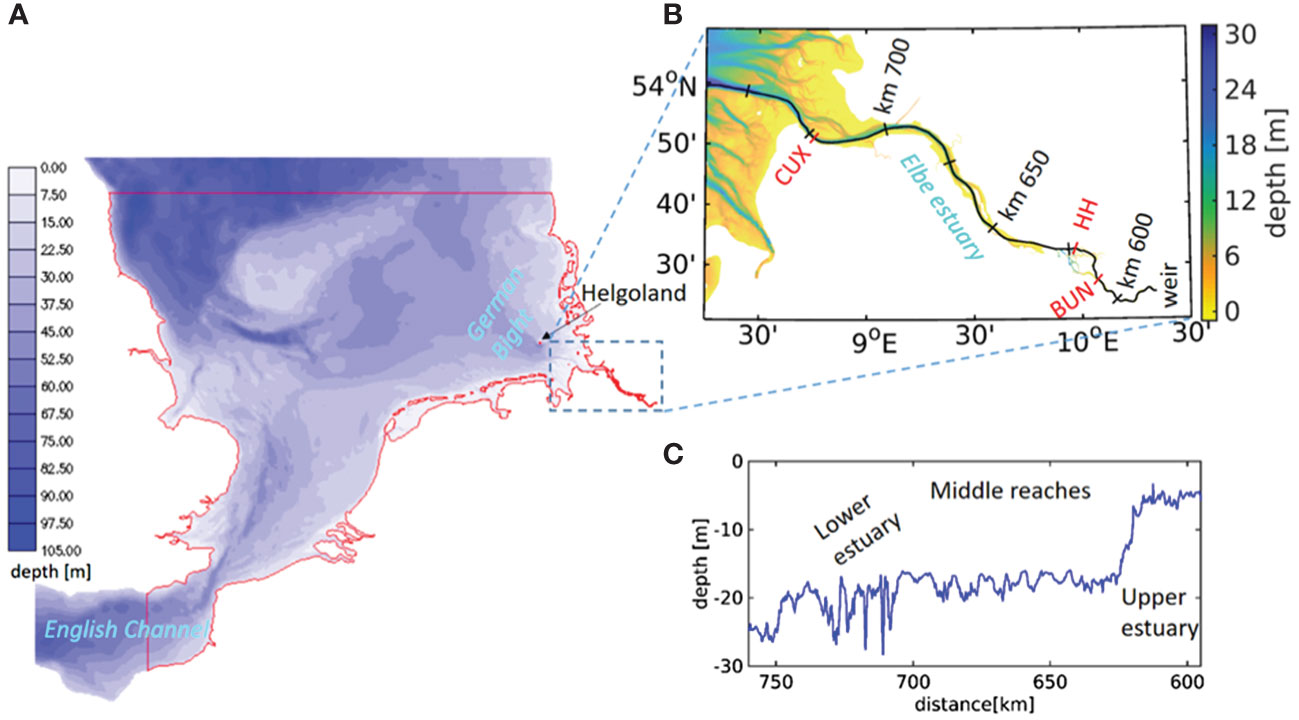
Figure 1 (A) Model domain of the southern North Sea with a three-dimensional (3D) domain marked by a solid red line; (B) the focal area of the Elbe estuary with bathymetric depth given as a background. Black bars indicate the official axial reference frame (kilometres from the Elbe river source). Red bars and labels indicate geographic locations used for dynamical analysis with labels indicating the station name (Cuxhaven: “CUX”, Hamburg St. Pauli: “HH” and Bunthaus: “BUN”); (C) the axial depth profile of Elbe estuary with the names of the axial compartment.

Human inventions transformed the former inland delta into a tidally dominated estuarine freshwater reach prone to hydrodynamic extremes. Not long after the construction of the tidal weir – but before the major deepening campaign of 1969/1970 – the Elbe estuary was ravaged by a catastrophic storm surge in February 1962 breaking dikes all along the estuary and up to the south-eastern part of the bifurcation area where numbers of casualties reached 222 in a single city district². After the disaster, dikes were moved closer to the estuarine channel and dike heights increased such that areas behind the dike line became safe but inter-tidal storage area was reduced. The modern Elbe estuary has hard-protected shorelines due to its role as a major waterway for large container vessels. Channel convergence at the mouth and in the middle reaches amplify the semi-diurnal tides (Winterwerp et al., 2013). The propagating tidal wave becomes a standing wave close to the bathymetric jump that functions as a partial reflector (Hein et al., 2021; Sohrt et al., 2021). This area is flood-dominated manifesting the estuarine maxima of the tidal range and turbidity due to fine and organic material (Pein et al., 2021). Downstream, the channel becomes ebb-current-dominated allowing for the export of particulates given that river runoff is high enough to flush the port region. Kerner (2007) reported a marked response of turbidity and oxygen levels to the comparatively modest channel deepening in 1999/2000. In the years after, a major river flood in June 2013 runoff has been low and turbidity in this area has increased (Weilbeer et al., 2021). This situation requires increased maintenance dredging, which is economically and ecologically costly. In summer 2022, dredging has been ordered to come to a halt after fish dying in the turbid and low-oxygen waters of the tidal freshwater reach. The modern Elbe estuary is, thus, in an unsustainable state, and the pressure for transformation is high. Global warming and MSL rise bring additional pressures, and, therefore, a local projection of future hydrodynamics including the quantification of scenario spread is a crucial step forward to inform effective adaptation planning.

In the present study, we use a cross-scale numerical model of the southern North Sea and Elbe estuary to dynamically derive the sea level, currents and associated variability of physical scalars in the Elbe estuary during 2090–2099 under the RCP8.5 scenario (Meinshausen et al., 2011). RCP8.5 assumes the growth of greenhouse gas emissions throughout the 21st century that results in a global surface temperature increase of 2.6°C–4.8°C for the 2081–2100 average, relative to 1986–2005 (Collins et al., 2013). While the likelihood of this emission pathway has been questioned (Hausfather and Peters, 2020), it remains scientifically useful for the high signal-to-noise ratio and is used here to characterize the emergent climate change signals. The aim of this study is to quantify the range of the hydrodynamic response to the end-of-century projected climate variability in the estuarine environment under an upper-end warming scenario. This includes the fact that a special focus is given to the scenario spread representing the climate variability. Here, we use the ensemble simulations to pinpoint the impact on the estuarine dynamics of the spread of global sea level rise vs. the one due to the internal variability of the climate system.

2 Methods

2.1 Downscaling concept

The RCM outputs based on the MPIOM-REMO model are available in hourly resolution for sea level and meteorological fields (Mayer et al., 2022b). MPIOM-REMO is a coupled framework of the Max-Planck-Institute for Meteorology ocean model and the REgional atmosphere MOdel (Elizalde et al., 2014). The model outputs of currents, salinity and water temperature are available at the monthly scale. For this reason, it is not feasible to directly drive the three-dimensional model of the southern North Sea and Elbe estuary (SNSE) with the outputs of the RCM ensemble simulations. Previous downscaling studies solved the issue by using a tidal model to drive vertical and horizontal tides at the model open boundary (e.g. Hermans et al., 2020). Here, we set up the coupling directly at the tidal time scale by first running a two-dimensional (2D) simulation of the southern North Sea (SNS) driven by the MSL, vertical tides and wind only to retrieve hourly barotropic horizontal velocities (see the workflow in Figure 2C). This intermediate step ensures a consistent representation of the propagation of the tidal wave into the child model and facilitates adding MSL change at the barotropic processing level. The horizontal mesh of the 2D simulation is mostly identical to the three-dimensional (3D) mesh, but the Elbe estuary has been cut off, and the open boundaries locate 150 km further to the West in the English Channel and 50 km further to the North in the central North Sea (Figure 2A). MSL change from the probabilistic projection is added to the bias-corrected hourly sea level variations from RCM at the open boundaries of the 2D domain. The MSL time series of the global MSL projection (Figure 2B) has annual resolution and is interpolated to hourly time steps. In order to preserve the hydrodynamics prescribed by the RCM, MSL change is imposed uniformly at the open boundary. The 2D model of SNS forced by MSL plus hourly sea level and wind fields from the RCM is integrated for 10 years. During model integration, the outputs of the sea level and barotropic currents are saved every hour to serve for the forcing of the 3D run. They are sampled along the open boundaries of the 3D domain (Figures 2A, C). At each vertical level, the horizontal velocities correspond to the sum of the hourly barotropic currents and the monthly depth-dependent currents. The latter have been sampled directly from the RCM and interpolated to hourly time steps before adding them to the hourly barotropic velocities. Lateral boundary data for temperature and salinity are sampled from the RCM outputs and interpolated onto the child model open boundary. In addition, salinity and temperature are forced in a 50-km-wide sponge layer with relaxation constants tending to zero towards the inner (landward) boundary of the sponge layer.

FIGURE 2

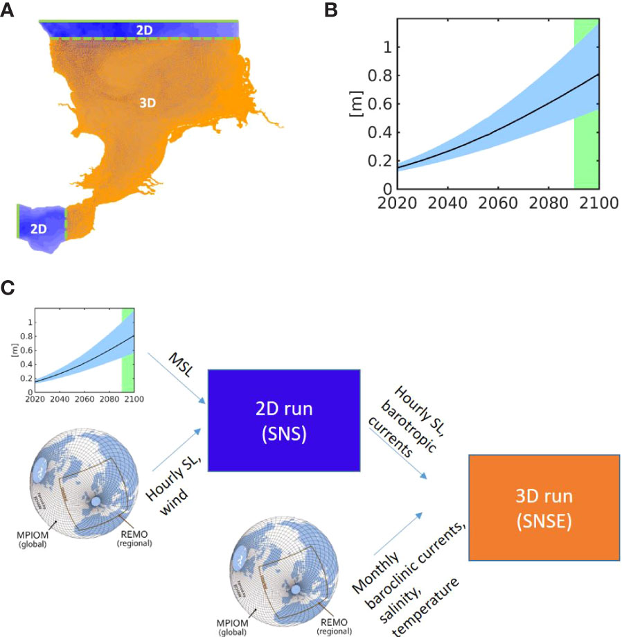
Figure 2 (A) Distribution of the two-dimensional (2D) and 3D domains. (B) Projected global mean sea-level rise under RCP8.5 regionalised for southern North Sea (Palmer et al., 2018) where the black solid line represents the median of projected mean sea-level rise at the model open boundaries and the blue-shaded area gives the spread between the 5th and 95th percentiles of projected global mean sea level (MSL) rise. The green-shaded area marks the period of model integration. (C) Workflow, whereas “SNS” refers to the 2D model covering the southern North Sea only, and “SNSE” refers to the 3D model covering the southern North Sea plus Elbe Estuary.

2.2 The estuarine model

For the simulation of the estuarine physics under climate change, we use the Semi-implicit Cross-scale Hydroscience Integrated System Model (SCHISM, Zhang et al., 2016). The SCHISM solves the Reynolds-averaged Navier–Stokes equation on an unstructured grid and has been successfully applied in numerous hydrodynamic and cross-scale studies (see, for example, Ye et al., 2020; Huang et al., 2022). Here, we rely on the modelling capacities developed for the area of the German Bight and its estuaries (Stanev et al., 2019). Building on the model mesh developed for the Elbe estuary (Pein et al., 2021), we have complemented the model area by a coarse representation of the adjacent SNS to better resolve non-linearities and feedbacks between the estuary and the shallow SNS (Figure 1A). The nominal horizontal resolution in SNS is 5 km and reduces to 1 km in the German Bight. The vertical mesh is the same as in Pein et al. (2021), which means that most of SNS is resolved by 21 sigma levels vertically except for the shallow Wadden Sea. The time step has been increased from 60 to 80 s because it is not critical for pure hydrodynamic simulation. Adding the SNS area to the Elbe estuary model facilitates the downscaling of the ocean and atmospheric variability over the SNS assuring both the downscaling and the upscaling of physical processes between the coastal ocean and the estuary in the area of the Elbe region of freshwater influence (i.e. the German Bight). The topography remains unchanged during model integration and represents the morphologic state in 2016. We assume that, during the current century, the shorelines remain protected by dikes and no flooding beyond the current dike line will occur. We note, however, that, unlike previous works (for example, Pelling and Green, 2014), this model experiment allows for the flooding and drying of the shallows in front of the dike line.

2.3 Global climate scenarios

The dynamical drivers in this study are 1) global MSL change and 2) coupled ocean–atmosphere variability. Global MSL rise is driven by the thermosteric expansion, the melting of polar ice caps and glaciers and the gravitational responses induced by the ice masses becoming liquid (Church et al., 2013; Golledge, 2020). Global MSL rise may be regionally exacerbated or mitigated by vertical land movements like postglacial isostatic rebound. For the prescription of MSL rise, here, we use probabilistic estimates under the RCP8.5 scenario from the UKCP18 project (Palmer et al., 2018; Palmer et al., 2020).

The coupled ocean–atmosphere dynamics have been sampled from regionalised simulations of the Max-Planck-Institute Earth System Model Low Resolution (MPI-ESM-LR) ensemble runs under the RCP8.5 scenario, where the downscaling of the global climate ensemble was performed by a regionally coupled climate system model with a nominal resolution of the hydrodynamic model of 5 km in the SNS (MPIOM-REMO, see Mikolajewicz et al., 2005; Mathis et al., 2015; Lang and Mikolajewicz, 2020; Mayer et al., 2022a). The resolution of the atmospheric module REMO is approximately ~24 km, and this model predicts, in addition to atmospheric variables, daily surface runoff, which serves as river input here. The ensemble simulation dataset represents changes in ocean density and currents as well as meteorological conditions including atmospheric water transport due to the enhanced radiative forcing under climate change. The ensemble is created by starting the global model from different historical states of the years 1950–1959 of three previous simulations with the same model system (Mathis and Mikolajewicz, 2020). For the downscaling of the global simulations, its 6-hourly outputs serve as a forcing for the MPIOM-REMO regional climate modelling framework, which, in turn, provides the boundary forcing for the SCHISM simulations analysed in this study. These ensemble simulations enable exploring the internal variability of the climate system by the variation of the initial states over the 30 ensemble members. They, however, do not include MSL rise, which is why it is added here in addition to the forcing data using the probabilistic estimates (Palmer et al., 2018; Palmer et al., 2020).

For the focus of this study on scenario spread, it is important to keep in mind that the spread of MSL roots in the variability of the global climate system while ensemble spread is due to internal variability due to local synergies and feedbacks between geometry, density distribution, wind and tidal forcing.

2.4 Model calibration and choice of ensemble members

For the scope of this exercise, an integration period of 10 years for one simulation is feasible. In order to represent the internal variability of the climate system, it is necessary to downscale at least a couple of ensemble members from the large ensemble. Out of 30 realisations provided by Mayer et al. (2022a), we have identified three runs representative of the 5th, 50th and 95th percentiles of monthly sea level variability at Cuxhaven that is located at the mouth of the Elbe estuary (Figure 1). The identification of representative ensemble runs involved two major steps. First, the time series of the 5th, 50th and 95th percentiles of monthly sea level at Cuxhaven was compiled from the complete set of ensemble RCM simulations. In the second step, the root-mean-squared distances between any ensemble run and each of the three compiled time series were calculated and the three ensemble runs with the smallest differences from any of the three compiled time series were selected. This subset of the three runs constitutes the model forcing, and the forced runs are indexed r1, r2 and r3 throughout this paper, representing the 5th, 50th and 95th percentiles of monthly MSL variability, respectively. The time series of the monthly sea level during 2090–2099 given by the RCM simulations and the choice of representative trajectories are illustrated in Supplementary Figure S1. The MSL at the open boundaries has been calibrated in such a way that during one year (1997) in the historical simulation period of the RCM (1950–2005, see Mayer et al., 2022a), the ensemble run representing the median (r2) matches the water level data at Cuxhaven, i.e. the sea level at the open boundary is bias-corrected at the 2D processing level, and the increment is used for the bias correction of the projection model runs. The observed MSL from 1997 to 2019 at Cuxhaven gauge serves as a general vertical reference setting the baseline for MSL rise from 2020 to 2100 (Figure 2B). The median ensemble run (r2) is also used for the calibration of the bottom drag coefficient in the region between the open boundaries and the Elbe estuary mouth. The child model is repeatedly run for 1 year of the historical period of the RCM simulation (1997) until the drag coefficient is such that the historical observed M2 tidal amplitude at Cuxhaven is reproduced by the model. Upstream from Cuxhaven, the parametrization of bottom drag is identical to Pein et al. (2021). By this means, it is assured that the projected estuarine dynamics under future climate forcing are consistent with the estuarine dynamics under historic conditions. However, we do not aim to provide a systematic evaluation of future vs. historic dynamics or a prediction of the future conditions. Rather, our goal is to construct reasonable dynamical projections that span a range of estuarine responses to future MSL change and internal climate variability.

2.5 Model experiments

Simulation runs are divided into two modelling experiment series (Table 1). One uses the median of regionalised for SNS global MSL rise (black solid line in Figure 2B) in combination with three realisations of the RCM ensemble simulations. The three ensemble members represent the 5th, 50th and 95th percentiles of monthly sea level variability at Cuxhaven in the mouth of the Elbe estuary in the RCM simulations (see map in Figures 1, S1). The second modelling experiment series comprises the median run from the first modelling experiment series plus two additional runs using the 5th and 95th percentiles of regionalised for SNS global MSL rise with the median RCM realisation. The three trajectories represent the 5th, 50th and 95th percentiles of regionalised global MSL change under the RCP8.5 (see Palmer et al., 2018) and serve to simulate the effect of the spread of projected global MSL change. The 5th–95th percentile range is equivalent to the likely range sea level projections presented in the last two IPCC Working Group I assessment reports (Church et al., 2013; Fox-Kemper et al., 2021). The sea level projections used here are similar to those present in the latest IPCC assessment report (see Weeks et al., 2023). The analyses are based on hourly model output data. For the tidal analysis and the computation of residual flows, the UTide package (Codiga, 2011) has been used. In the following, we first present the response in the area of the SNS to frame the associated estuarine dynamics elucidated in the following results section. We refer to the sea level or MSL/MSL outside the estuary and water level/MWL inside the estuary owing to its character of a land–sea transition zone. Throughout the study, the averaging and stipulation of maxima refer to the monthly mean or maximum values if not otherwise stated. Spread refers to the difference between the 5th and 95th percentiles of MSL change and the RCM ensemble runs, respectively.

TABLE 1

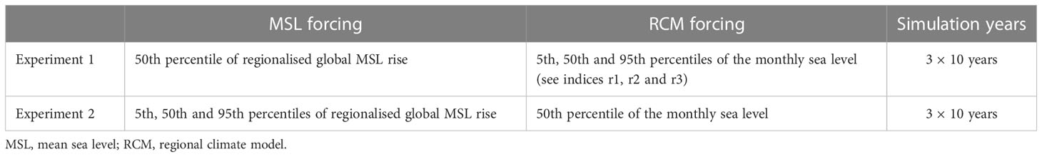
Table 1 Summary of model experiments that are defined by combining different representative trajectories of the projected mean sea level and regional climate model simulations.

3 Results

3.1 Dynamical downscaling towards the Elbe estuary

The MSL and seasonal and tidal variability in the Elbe estuary are governed by respective dynamics in the North Sea and German Bight. The expectation is that these signals become amplified by the funnel-shaped geometry and horizontal buoyancy gradients of the German Bight and the Elbe estuary. It is, however, unclear, if the variability and trends manifesting at the borders of the southern North Sea reach the German Bight in a spatially coherent manner and what the magnitude of the response in the Elbe estuary region is.

Figures 3A–D show the climatologies of the monthly sea level, M2 tidal amplitude, sea surface salinity and temperature at the model open boundary in the English Channel (see Figure 2A) for each of the three ensemble members. The annual range of the monthly sea level attains 0.17 m, whereas the annual cycle is fairly similar in the three realisations (Figure 3A). The ensemble spread of the M2 amplitude is comparatively small both in comparison with its annual range and with the ensemble spread of the monthly sea level (Figure 3B). The monthly sea level and M2 amplitude are weakly anti-correlated. Surface salinity demonstrates freshening during the spring and summer following loosely the variations of the monthly sea level (Figures 3A, C). Unlike surface salinity, the spread of sea surface temperature is small and the seasonal cycle is similar to the one of the M2 amplitudes. At Cuxhaven, the monthly sea level, tidal amplitude, surface salinity and temperature show mostly positive correlations with respective variations at the English Channel open boundary (Figures 3E–H). Enhanced vertical excursion of scatter points indicates the amplification of monthly sea level variations between the open boundary and the estuary (Figure 3E). The variability of the monthly M2 tidal amplitude is also increased, although average amplitudes are smaller owing to frictional control in the shallow waters (Figure 3F). Elbe mouth surface salinity demonstrates large excursions revealing the variations of freshwater fluxes (Figure 3G). The upper-end realisation manifests a distinct cluster of high salinities in the Elbe estuary mouth associated with relatively low salinities at the open boundary (see “r3” with 12–22 g kg^-1 over 34.2–34.3 g kg^-1, Figure 3G). Surface temperature follows a hysteresis-like pattern indicative of a phase lag during the warming and cooling of the coastal strip with larger (smaller) ensemble spread during winter and summer (spring and autumn) (Figure 3H). Thus, in a first simple approximation, the hydrodynamic response at the mouth of the Elbe estuary is a linear function of variability at the western open boundary. The range of the near-mouth response is high for salinity and the M2 amplitude revealing the importance of local processes and internal variability.

FIGURE 3

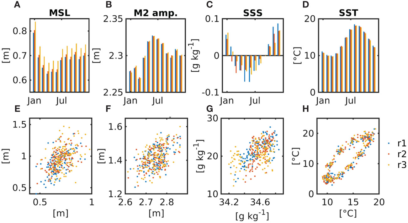
Figure 3 Monthly climatology of (A) the mean sea level (“MSL”), (B) the M2 tidal amplitude of the water level, (C) the anomaly of sea surface salinity (“SSS”) and (D) sea surface temperature (“SST”) in the English Channel. The scatter plots in the second line represent the relationship between the daily averages of the MSL, u, SSS and SST at the mouth of the Elbe estuary (Cuxhaven, see Figure 1B) relative to the English Channel variability. The three colours of the bars in (A–D) and dots in (E–H) refer to the three downscaled RCM ensemble realisations that are indexed r1, r2 and r3 in this study.

The ensemble-averaged MSL during 2090–2099 shows a strong zonal gradient in the northern part of the model domain between the Dogger bank and the North Frisian coast where water is piling up to an average level of ~0.88 m (Figure 4A). There is a similar, however, much-smaller set-up of water at the Dutch and East Frisian coast that increases towards the mouth of the Elbe estuary. The zonal pattern of surface elevation has been revealed by previous climate projection downscaling exercises (Hermans et al., 2020) and is explained by zonal winds driving water masses into the German Bight where they pile up in the area of Cuxhaven (Dangendorf et al., 2013a). Our simulations add further details to previous modelling efforts in particular along the Wadden Sea coasts where flooding and drying lead to a slightly reduced elevation near off-shore and enhanced sea level gradients locally (Figure 4A). The simulated pattern of tidal range during 2090–2099 is very similar to well-known historic dynamics (Figure 4B, see, for example, Stanev and Ricker, 2020). The maximum tidal range occurs in the English Channel and reduces steeply downstream of Dover Strait towards the amphidrome between East Anglia and the Dutch coast. A second region with weak tides is located off the Danish coast. On the English coast and in the German Bight, the tidal range rises sharply and reaches meso- or even macro-tidal levels.

FIGURE 4

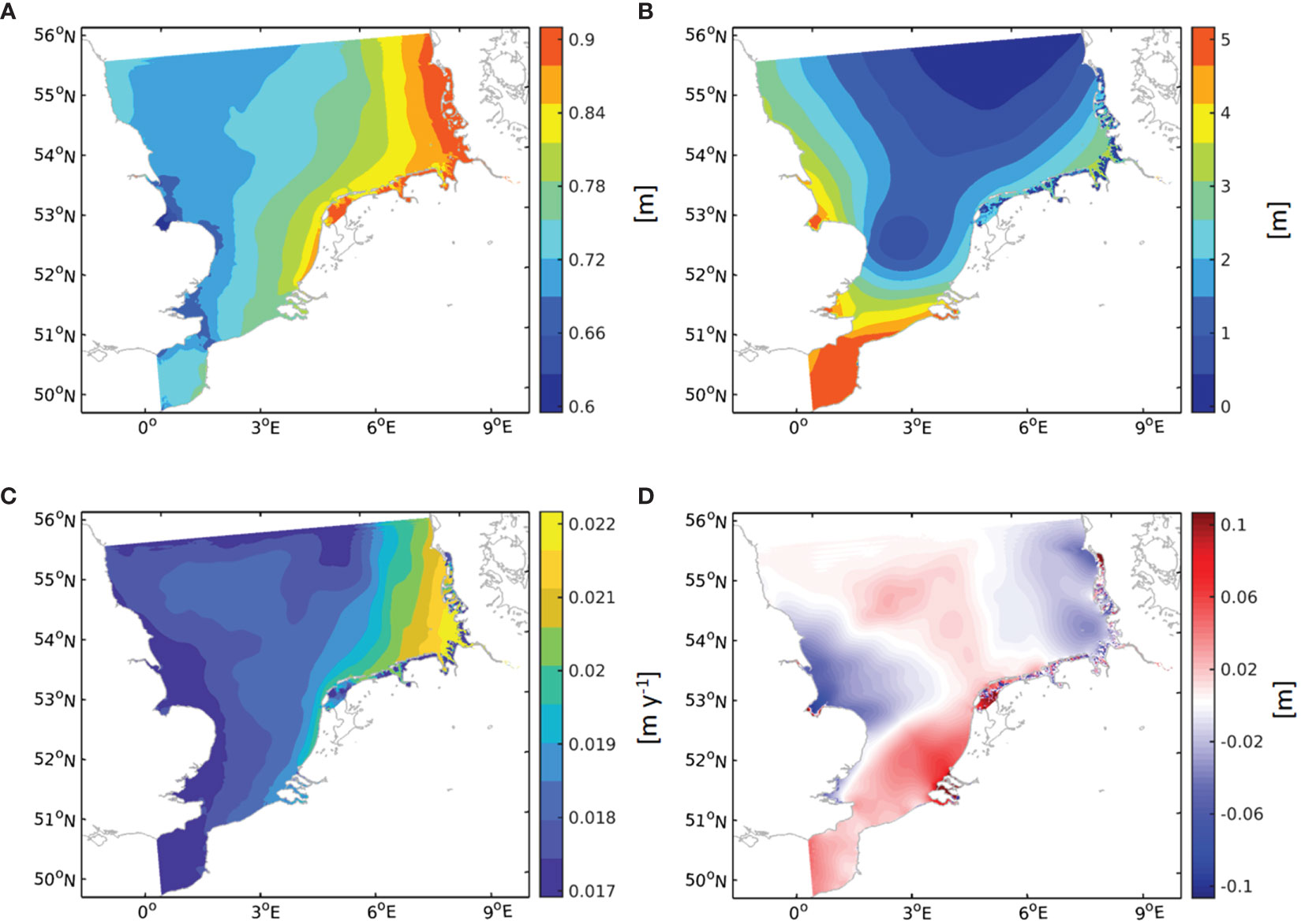
Figure 4 Simulated ensemble-averaged (A) MSL, (B) mean tidal range, (C) annual change of the MSL and (D) spread of tidal range due to the spread of MSL rise during the simulation period 2090–2099.

The trend pattern of MSL change partially replicates the pattern of MSL proper with maximum rates of ~22 mm y^-1 at the Elbe estuary mouth and background rates of ~18 mm y^-1 in central SNS (Figures 4A, C). Above-average MSL rise also occurs at the Dutch coast (19–20 mm y^-1), while the smallest rates manifest in the English Channel and at the East Anglian coast. Figure 4D shows the spread of the tidal range associated with the difference between the 5th and 95th percentiles of MSL change (see projected MSL change and spread in Figure 2B, Experiment 2 in Table 1). The mean surface elevation difference within the ensemble simulations of 0.56 m induces a relatively subtle response of ~ 0.05 m on the average of tidal range (Experiment 1 in Table 1, see Supplementary Figures S2C, D vs. Figures 2B, 4D). Under the upper-end MSL rise trajectory, tidal range increases in the area of the English Channel and in the area of Dogger Bank while decreasing north of East Anglia and in the German Bight. The simulated pattern is similar to the one presented by Schindelegger et al. (2018) for an MSL rise of 0.5 m with differences in the German Bight and in the north of the English Channel. The reduction of the tidal range in the north-eastern German Bight was also found by another modelling study applying a sea level rise of 0.8 m (Rasquin et al., 2020). Apart from this major difference with the changes reported by Schindelegger et al. (2018), the magnitude of changes is comparable with their study, which are both in the range of a couple of centimetres. Supplementary Figure S3A gives an overview about the vertical referencing of the scenario simulations in terms of MSL and tidal range in relation to the local bathymetry as well as a simple comparison between a supplementary simulation for a historic period and historic observations of the sea level at Cuxhaven station (Figure 1B).

Dynamical downscaling of the climate scenario shows that the Elbe estuary is located in a region of enhanced sea surface elevation demonstrating above-average rates of MSL rise (Figures 4A, C). The combination of rising sea levels, strong tides and a high local spread of projected sea level measures motivates a more detailed study of the hydrodynamic response inside the Elbe estuary to the applied climate projection forcing, which is the subject of the remainder of this paper.

3.2 Response of estuarine water levels to future mean sea level change and tidal forcing

In the Elbe estuary, ensemble-averaged MWLs increase from the mouth of the estuary in the upstream direction perpetuating the zonal gradient at the west coast of the German Bight (Figures 5A, 4A). Increase is gentle and linear up to km 615 to rise steeply upstream in the area of the shallow upper estuary. In Figure 5, the range of the estuarine response related to the spread of MSL change (Figure 2B) and ensemble spread (Figure S1) are given as the root-mean-squared differences between the ensemble runs representative of respective 5th and 95th percentiles, respectively. Spread by MSL rise dominates the range of projected MWLs in the outer estuary and middle reaches until km 615 (Figure 5A). Upstream, spread by internal variability becomes more important overtaking the impact of MSL rise–related bandwidth at the tidal weir. Thus, mean water elevation and permanent flooding depend overwhelmingly on the course of MSL change in a warming climate. In the shallow upper reach, factors driven by internal variability, for example, river runoff, gain importance and are responsible for the increasing internal variability impact in the shallow upper reach.

FIGURE 5

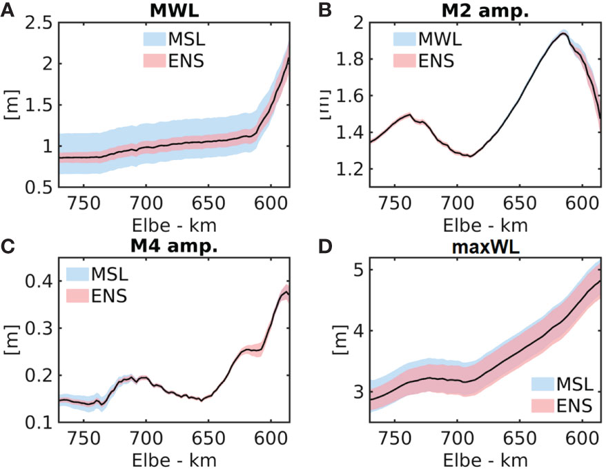
Figure 5 Axial profiles of the mean water level (MWL; black solid line) and model spread representing the difference between the 5th and 95th percentiles of MSL rise (“MSL”, bluish area) and the difference between the highest- and lowest ensemble members (reddish area, “ENS”), respectively, are given for the estuarine (A) MWL, (B) mean M2 amplitude, (C) mean M4 amplitude and (D) monthly maximum water level (maxWL).

The bandwidth of the projected M2 tidal amplitude is an order smaller than the one of the estuarine MWL and spread reaching merely 0.05 m the shallow upper estuary (Figure 5B). Under the future climate forcing, the along-channel profile of the M2 amplitude remains largely identical to the historic one showing two maxima, one near the estuarine mouth and one in the area of the port of Hamburg (see, for example, Stanev et al., 2019; Hein et al., 2021; for locations, see the map in Figure 1B). The bimodal axial profile of the M2 tidal amplitude is likely due to the axial variance of channel convergence (Winterwerp et al., 2013) and constitutes an important benchmark for the simulation of tides in the Elbe estuary. Upstream from Hamburg, the main lunar tide is drastically reduced due to both the friction and partial reflection of the tidal wave at the transition from the deepened middle reaches to the shallow upper estuary (Figure 5B; Sohrt et al., 2021). In the upper 20 km of the channel, ensemble spread overtakes the bandwidth engendered by the spread of MSL rise and the range of the projected M2 tidal amplitude becomes comparable to the range of projected MWLs (Figures 5A, B). The amplitude of M4 overtide reveals a similar response, but it is dominantly controlled by the spread of MSL in the lower estuary and internal variability in the upper estuary, respectively (Figure 5C). Since M4 is known to shape tidal asymmetry, a preliminary conclusion is that the bandwidth of the future of tidal asymmetry in the upper estuary and port area is rather controlled by internal variability than by the uncertainty of the projected MSL rise.

Extreme estuarine water levels during the 2090–2099 simulation period are represented by the time-averaged and ensemble-averaged monthly maximum water levels (maxWLs) (Figure 5D). The axial profile of the monthly maxWLs follows the one of the M2 amplitude in the lower estuary. Upstream from the port of Hamburg, however, the maxWLs are not attenuated in the same fashion as semi-diurnal tides but they continue to rise steeply by ~ 0.012 m km^-1 towards the tidal weir. Although, herein, we do not intend to make quantitative comparisons between the past and the future, a compilation of long-term mean and mean monthly maxWLs from gauge observations along the Elbe estuary demonstrates very similar historical along-channel profiles as the future simulations. This underlines the decisive role of the geometry in shaping the estuarine response to marine forcing (see Supplementary Figure S3B). According to the simulations, in the lower estuary, the ensemble spread of the monthly maxWLs attains 84% of the bandwidth related to MSL spread, e.g. at Cuxhaven, the 10-year average range of monthly maxWLs is 0.46 and 0.55 m due to the internal variability and spread of projected MSL, respectively. In the shallow upper estuary, ensemble spread becomes even more important reaching 102% of the bandwidth of uncertainty of MSL at Bunthaus. This means that the uncertainty of extreme water levels is approximately equally controlled by projected MSL and internal variability. Thus, internal variability may produce extreme trajectories that possibly exacerbate the upper-end scenario of MSL rise. Furthermore, the local range of estuarine extreme monthly water levels exceeds the spread of MSL applied at the model open boundaries illustrating the value of numerical downscaling in comparison with the ‘bathtub method’.

Having assessed the projected mean axial profiles and scenario spread of estuarine mean water elevation, tides and extreme water levels, the emerging question is how the estuarine response forms over time at different characteristic locations along the estuary, like the mouth (Cuxhaven), port area (Hamburg) and beginning of the shallow upper reach (Bunthaus) (locations see Figure 1B). Following the ratio of Figures 3E, F or even the ‘bathtub method’, the expectation is that all of them are positively correlated with the decadal trend of the MSL change of +12.1 mm y^-1 that is imposed at the open boundary (Figure 2B) and that increases towards the German Bight (Figure 4C). Results show the averaged rates of increasing MWL at the four stations between 18.7 and 22.5 mm y^-1 exceeding rates in the central and eastern SNS (Table 2, for locations, see Figure 1A). The time series of MWL change at the four stations are illustrated in Figures 6A–D. They demonstrate the spread of global MSL rise dominating the spread of projected future MWLs. In the upstream stations of Hamburg and Bunthaus, however, the ensemble spread reaches more than 47% (Hamburg) and up to 66% (Bunthaus) of the projected MSL-related bandwidth (Figures 6C, D). At the same stations, MWL change is far from constant but stagnates or even decreases during 2090–2094 to rise quickly between 2095 and 2099. This result emphasizes the value of long-term observations (assessing past MSL change) and simulations to detect inter-annual variations in response to climatic change and decadal variability. M2 tidal amplitudes increase moderately at the off-shore station Helgoland growing more rapidly within the estuary and, in particular, at the upstream stations (Table 2 and Figures 6E–H). The increase is partially due to the variations of the M2 amplitude with the nodal tide, which is on the increase during 2089–2098, whereas the nodal increase at Cuxhaven is approximately 4 mm y^-1 in the RCM simulations (not shown). At Hamburg and Bunthaus stations, the quick increase of the M2 amplitude occurs during the period of stagnating or retreating mean surface elevation, whereas, during fast MWL rise after 2095, the increase of the M2 amplitude slows down (Figures 6G, H). This antagonism between the response of the M2 amplitude and the MWL is most obvious at the Bunthaus station. The same location also reveals the largest bandwidth of the projected M2 amplitude, which is overwhelmingly dominated by the spread of global MSL rise until 2097 (Figure 6H). At Helgoland and Cuxhaven stations, the ensemble spread of the M2 amplitude is more significant than upstream showing similar (Helgoland) or greater (Cuxhaven) breadth as spread due to the uncertainty of projected MSL rise (Figures 6E, F). We note here that the different evolution of the trends of MWL and M2 amplitude (or tidal range) in the upper estuary is not a new revelation, but historical observations showed an analogous response of the tidal amplitude and high water (increase) vs. the MWL and low water (decrease) following channel deepening (Weilbeer, 2014).

TABLE 2

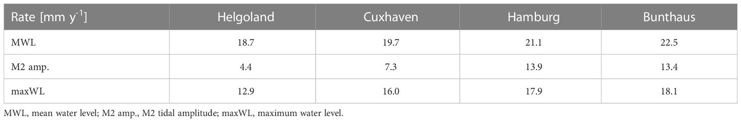
Table 2 Decadal ensemble-averaged rates of change of the annual mean water level, monthly M2 tidal amplitude and monthly maximum water level at four stations off-shore and within the Elbe Estuary.

FIGURE 6

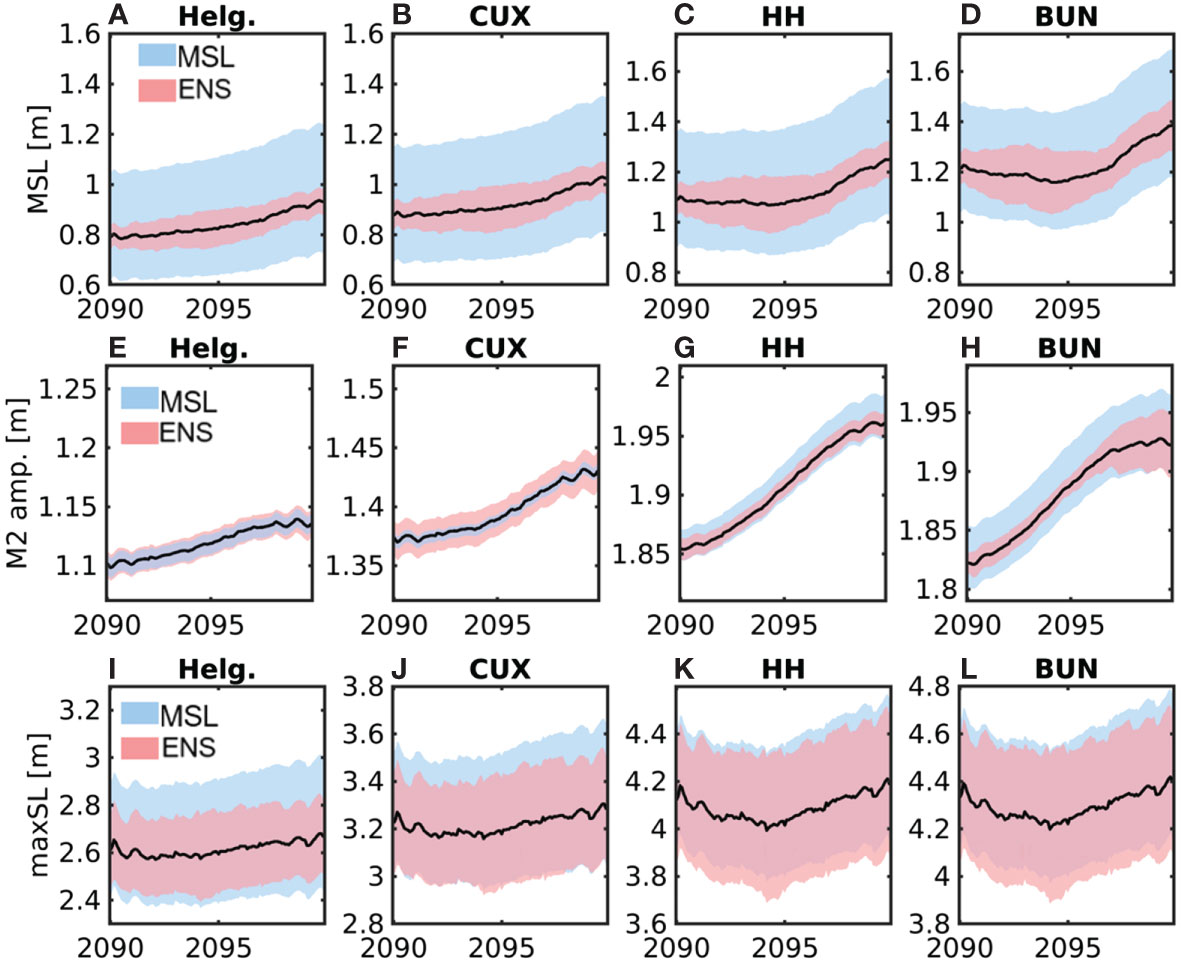
Figure 6 Time series of the median trajectory and the spread representing the difference between the 5th and 95th percentiles of MSL rise (bluish area, “MSL”) and the difference between the lower- and higher-end ensemble runs (reddish area, “ENS”), respectively, are given at four stations for (A–D) the MWL, (E–H) mean M2 tidal amplitude and (I–L) monthly maxWL. The time series have been smoothed using a moving average window of 48 months for greater clarity.

The axial trend of monthly maxWLs intensifies in an upstream direction same as MWLs (Table 2). Increase is steady at all stations (Figures 6I–L), which implies that extreme water levels follow either the rise of mean water elevation or increasing tidal range but neither do stagnate nor reduce (Figures 6C, D, K, L). In the lower estuary, the spread of maxWLs related to the spread of projected MSL rise is larger than spread of MWLs (Table 2 and Figures 6B–D, J–L). The range becomes larger at all four stations in the second half of the decade, replicating the trend manifestation in MWLs (Figures 6A–D, I–L). Ensemble spread is particularly important at the two upstream stations (Figures 6K, L). The conclusion is that tides, mean and extreme water levels overall get amplified by global MSL rise, but the local trajectories of the tidal amplitude and MWL accelerate at different times demonstrating opposite trend changes in particular close to the head of the estuary. The range of projected monthly maxWLs exceeds not only the one of the tidal amplitude but also MWLs with significant bandwidth related to internal variability in particular in an upstream direction. These locations are prone to the most extreme water levels while demonstrating large spread both due to the uncertainty of future sea levels and internal variability.

3.3 Internal variability and extreme water levels

The large spread of the extreme water levels related to internal variability motivates a closer look at the timing and location of extreme events and how they are associated with average monthly water levels and tides. An overview of respective dynamics in the three ensemble simulations is given in the supplementary material (Supplementary Material Figure S4) whereas ensemble-averaged seasonal ranges are represented in Figure 7. The Hovmoeller plots of the anomalies of monthly MWLs, monthly M2 tidal amplitude and monthly maxWLs show that seasonal variability dominates the subtidal dynamics, including the variations of the M2 amplitude in the lower and middle reaches (see location in Figure 1). Along this channel section, anomalies fluctuate synchronously. Upstream, i.e. in the shallow upper estuary with reduced channel depth and diameter, dynamics change drastically with the range of monthly MWLs increasing from ~0.6 m to more than 1 m at the tidal weir (Figure 7 and Supplementary Figures S4A, D, G). The oscillations of the M2 amplitude also become more vigorous in this region (Figure 7 and Supplementary Figures S4B, E, J). Similar to the inter-annual trends at the Bunthaus station (Figures 6D, H), the monthly M2 amplitude is anti-correlated with the monthly MWL while the monthly maxWLs are mostly positively correlated with the monthly MWL (Supplementary Figure S4, see also next sub-section 3.4). The most extreme water levels occur at the tidal weir (Figure 7), and the Hovmoeller presentation indicates that they propagate seaward in time. Approximately once a year and in each of the three runs (Experiment 1, see Table 1), the extreme water levels occur for the whole estuary synchronously, while the timing is different between realisations.

FIGURE 7

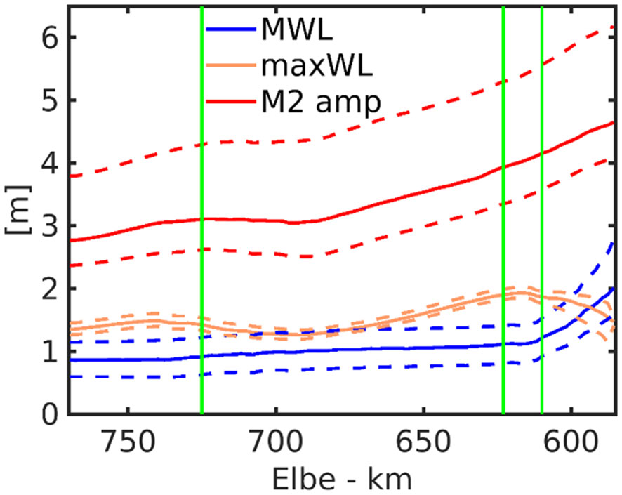
Figure 7 Axial seasonal ranges of monthly mean (MWL, dashed blue lines) and monthly maximum (maxWL, dashed blue lines) water levels and the monthly M2 amplitude (dashed orange lines), whereas the lower (upper) dashed lines represent the ensemble-averaged 5th (95th) percentiles, respectively. The thick solid lines show the ensemble-averaged median, whereas the thin green lines mark the axial positions of Cuxhaven, Hamburg and Bunthaus stations, respectively.

For a better understanding of timing and magnitude, the time series of monthly MWLs, the monthly M2 amplitude and monthly maxWLs have been sampled at Cuxhaven and Bunthaus stations (Figure 8, see geographic locations in Figure 1). The time series sampled at the mouth of the estuary illustrates the variability of monthly mean water elevation and the monthly M2 amplitude (Figures 8A, E). High winter monthly water levels are associated with a low M2 amplitude, whereas often extreme maxWLs coincide with high monthly water levels (Figures 8A, B). An exemplary extreme event happens at the end of 2091 in the lower-end ensemble run that is related to a maximum of monthly westerly wind magnitude (see the blue triangle for timing, Figures 8B, F). This extreme event occurs at both stations and represents the absolute maximum of the realisation (r1) with the peak water level exceeding 6 m at the Bunthaus station (Figure 8D). An exemplary extreme event from the median realization (r2) happens at the end of 2098, when the extreme water level at both stations coincides with a high monthly water level and a peak of monthly zonal winds (see the red triangle for the timing, Figures 8B, D, F). Finally, an exemplary extreme event from the third ensemble realization (r3) occurs in early 2099 with the water level in the Bunthaus station reaching 5.1 m (Figure 8D), while the water level at the Cuxhaven station remains moderate attaining merely 3.55 m (Figure 8B). At the time of the extreme water levels at both stations, the M2 amplitude has a pronounced minimum at the Bunthaus station (Figure 8G) while river Elbe discharge, monthly westerly wind magnitude and monthly MWLs have maxima, respectively (Figures 8H, F, C). The coincidence between a high monthly water level and a maxWL suggests an important role of monthly MWLs representing a “seasonal baseline” for monthly extreme water levels playing a role comparable to global MSL rise (the “global baseline”). Wind magnitude is an important driver of extreme water levels up to the shallow upper estuary. In the upper estuary, high river discharge damps the M2 magnitude while positively interacting with increased wind speed from westerly directions such that extreme compound events may occur locally.

FIGURE 8

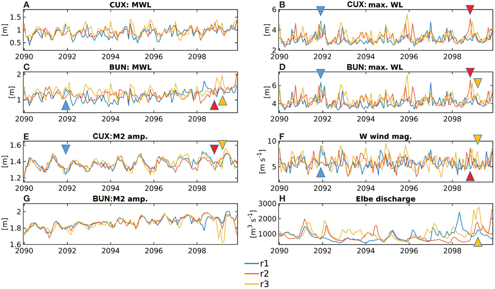
Figure 8 Time series (A, C) monthly MWLs, (E, G) M2 tidal amplitude, (B, D) monthly maximum water levels at (A, B, E) the Cuxhaven station (“CUX”, Figure 1B) and (B, C, D) Bunthaus station (“BUN”, Figure 1B). (F) shows monthly mean westerly wind magnitude at Helgoland (Figure 1A) and (H) gives monthly averaged of river discharge at the tidal weir. The coloured triangles mark the timing of an exemplary extreme event in the respective ensemble run (realisations r1, r2 and r3 are color-coded).

3.4 Signal response relationships under fast mean sea level rise

The monthly maxWLs at the Bunthaus station respond both to sea-born storm surges and river flood, while underlying seasonal water levels seem to anticipate extreme water levels. We may ask if these relationships respond to fast decadal MSL rise and if the estuarine response reveals the interference of the global tendency with internal variability. A scatter plot shows that higher monthly water levels associate with a lower M2 amplitude at the Bunthaus station (Figure 9A), confirming the general impression given by Figures 8C, G. Linear regression over the three ensemble simulations for the period of 2090–2094 and 2095–2099 demonstrates a weak linear anti-correlation of the M2 amplitude and monthly water levels (Figure 9A). This means that, under a rising sea level, the inversely proportional relationship between the semi-diurnal tide and seasonal water level variations becomes slightly more systematic. The monthly maxWLs, on the other hand, reveal a positive correlation with the monthly MWL at the Bunthaus station with the correlation coefficient R ~ 0.64 (Figure 9B). The regression line becomes less steep for the second half of the decade indicating that seasonal variations – that are subject to large spread by internal variability – tend to lose control of extreme water levels by MSL rise. Figures 9C, D illustrate the control of MWLs and extreme water levels by monthly westerly winds, with R = 0.64 and R = 0.68, respectively, during 2090–2094. The decrease of linear correlation for the period 2095–2099 implicates the weakening of the linear relationship between zonal winds and estuarine water levels. Since wind variability is a function of large-scale atmospheric pressure differences, which, in turn, depend on long-period processes such as the North Atlantic Oscillation, the weakening of the influence of zonal winds on estuarine water levels may indicate the reduced importance of internal variability during progressing climate change. However, significantly longer simulation times are required to substantiate this statement.

FIGURE 9

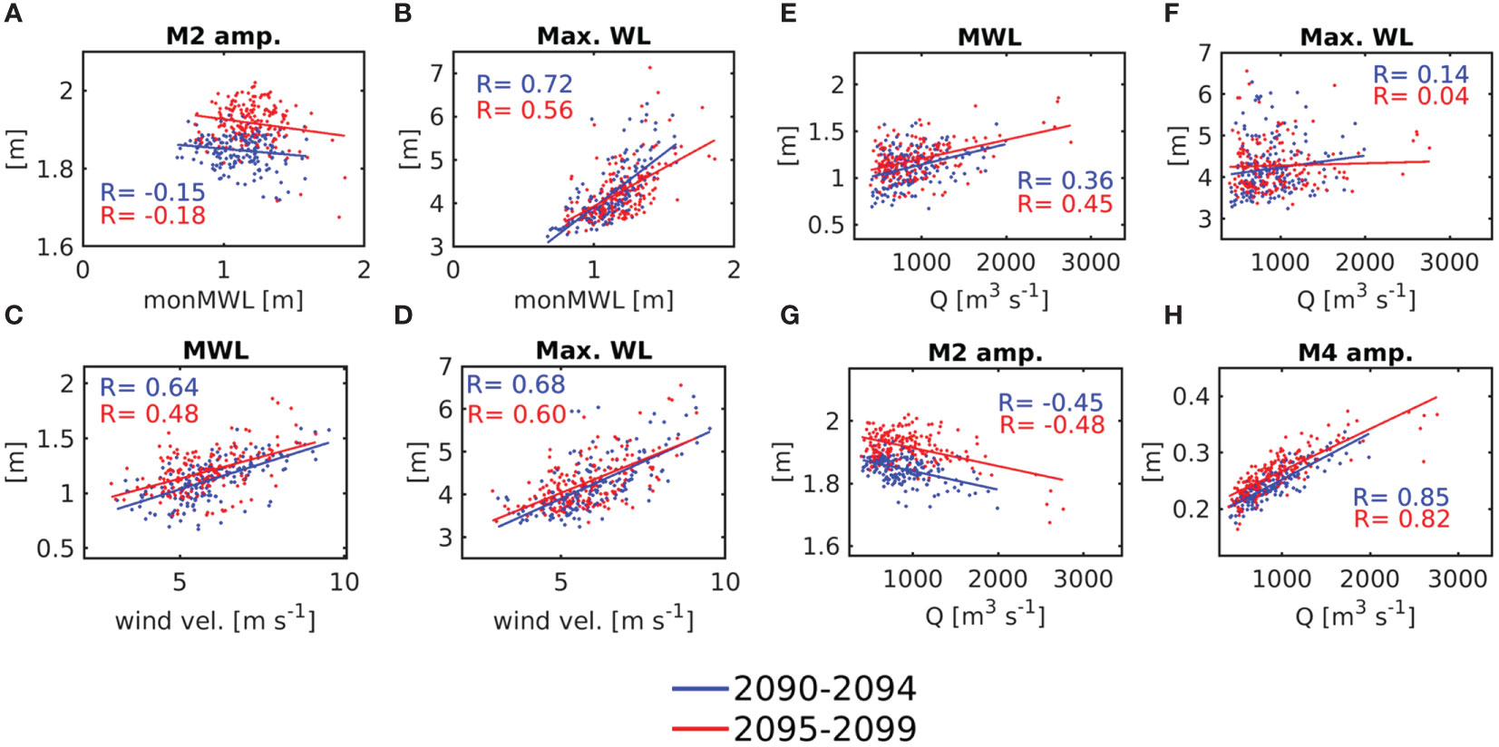
Figure 9 Scatter plots and linear regression illustrating the change at the Bunthaus station between the first and second half of the simulation period of the relationship (A) M2 tidal amplitude over the monthly MWL, (B) the monthly maximum water level (Max. WL) over the monthly MWL, (C) the monthly MWL over monthly westerly wind magnitude, (D) the monthly max. WL over monthly westerly wind magnitude, (E) the monthly MWL over monthly river discharge, (F) the monthly max. WL over river discharge, (G) monthly M2 tidal amplitude over monthly river discharge and (H) monthly M4 tidal amplitude over monthly river discharge.

While it is well-known that wind is the dominant driver of both monthly MWLs and surges, especially in the lower and middle estuarine reaches, Figures 8D, H give an example of extreme water levels occurring at the Bunthaus station during high monthly river discharge. Indeed, river discharge controls the water level in the upper estuary including the Bunthaus station and their positive linear relationship tends to reinforce during the decadal simulations (Figure 9E) decoupling from background MSL rise. The impact of runoff on maximum monthly water levels is not as clear (Figure 9F). Regression demonstrates a slightly positive correlation, but linear correlation coefficients are small indicating the insignificance of the linear relation (R < 0.15, Figure 9F). However, scatter points cluster both at very low and very high river discharge and a preliminary interpretation is that high river discharge can lead to a surge at Bunthaus, but the surge may also happen at particularly low river discharge. At moderate river runoff, monthly maxWLs appear to be less extreme. High river discharge tends to dampen the M2 tidal amplitude while enhancing the M4 amplitude in the shallow upper estuary (Figures 8G, H, 9G, H). The dampening of the M2 tide occurs not only during high river discharge at the upstream station but also during seasonally high MWLs at the mouth of the estuary (Figures 8A, E). This implies that other drivers than river flow disperse tidal energy. Dangendorf et al. (2013b) showed that seasonal MSL variability in the German Bight is mainly driven by atmospheric variability with increasing wintertime zonal wind activity enhancing seasonal MSL maximum. Additional forcing of the tidal currents by wind leads to higher bottom stresses outweighing the reduced effect of bottom friction due to higher water levels (Jones and Davies, 2008). This process can explain the coincidence of seasonally high mean and maximum monthly water levels and wind speed with a weakened M2 tidal amplitude. Indeed, we find a subtle linear anti-correlation between the local M2 amplitude and the zonal wind magnitude of R = - 0.3 at Bunthaus during 2095–2099 (not shown).

3.5 Response of currents, salinity and vertical mixing

The results and analysis presented in sections 3.3 and 3.4 addressed the drivers of the variability of the projected sea level and the magnitude and timing of simulated extreme events. The shallow upper estuary demonstrated volatile and extreme average and monthly maxWLs with the bandwidth of extreme water levels dominated by ensemble spread, i.e. the internal variability of the climate system. Even if the effect of internal variability of the climate system attenuates during fast decadal MSL rise under a high-emission scenario (Figure 2B), it may still contribute to coastal hazards in particular in combination with a high emissions/warming scenario of global MSL change (Figure 2B). A tentative conclusion is that, as MSL rise is progressing along the upper-end trajectory, extreme water levels do not necessarily increase but they still become more likely.

Coastal defence structures are the more visible part of the estuarine geometry, but they affect hydrodynamics only at the peak of extreme events. For the shaping of the estuarine response and the on-set of extreme events, the geometry below sea level is crucial, i.e. the width and depth of the channel, convergence and any constrictions that may lead to the amplification or damping of flows. The development and control of the estuarine response are subject to hydraulic engineering measures, morphological development, sediment management and possibly biological feedback effects. Although no coupled modelling was carried out for this study, we will briefly discuss the range of the estuarine response in the water column as this provides initial implications for pressures on sedimentary and biological subsystems. The knowledge and understanding of the internal response, i.e. baroclinic and other high-order processes, are crucial for the development of adaptation strategies to MSL rise. These processes, in particular, govern the transport of particulates and vertical mixing of dissolved substances such as nutrients and oxygen.

An important boundary condition to the oceanic and estuarine transport of particulates is given by the tidal current asymmetry. A rule of thumb is that the direction of tidal current asymmetry, flood or ebb domination controls the direction of transport of particulates. The tidal asymmetries respond both to MSL change and the internal variability of the climate system (not shown). The Elbe estuary was typically ebb-dominated in historic times. According to the modelling experiments (Table 1), the estuarine axial pattern of tidal current asymmetry is quite insensitive to the spread of MSL rise or internal variability (Figure 10). At km 660, simulated spread is such that the magnitude of the ratio of maximum flood to maximum ebb currents could change from below to above unity or vice versa. At these locations, the direction of tidal current asymmetry may thus change signs under climate change or due to internal variability. Compared to the seasonal range of tidal current asymmetry, these changes appear small and, by far, not indicative of a regime shift (Figure 10). Still, even subtle shifts of tidal current asymmetry may affect the sedimentary and biological subsystems at longer time scales. These issues require coupled modelling and will be addressed in a follow-up study.

FIGURE 10

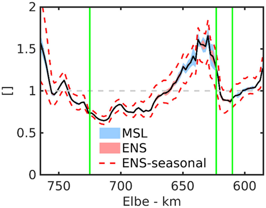
Figure 10 Ratio of maximum flood currents to maximum ebb currents (tidal current asymmetry) along the Elbe estuary, where the black solid line represents the ensemble average and the blue (red)-shaded areas represent spread under different rates of MSL rise (ensemble spread, i.e. internal variability). The dashed red lines represent the seasonal spread of tidal current asymmetry in terms of the ensemble-averaged 5th and 95th percentiles of the monthly time series of the current ratio along the estuarine channel. The solid green lines mark the axial positions of Cuxhaven, Hamburg and Bunthaus (Figure 1B).

The water column response to MSL rise and internal variability is systematic and provides further insight into potentially compensating trends induced by the two forcing signals (MSL rise vs. internal variability). Ensemble-averaged and time-averaged horizontal current velocity magnitude |u| reveals the most vigorous flows in the lower estuary, between km 670 and km 740, where average surface flows reach ≥ 1 m s^-1 (Figure 11A). Upstream, average flow speed diminishes reaching an estuarine minimum close to the bathymetric jump (Figure 11A). In the shallow upper estuary, average flow speed reaches levels comparable to the lower estuary. The vertical shear of the horizontal velocities is most pronounced downstream of km 670 marking the average position of the salinity front and of the two-layer exchange flow (Figure 12A and Supplementary Figure S5A). The response of the estuarine currents to the imposed MSL rise appears straightforward, demonstrating average positive rates of change over the entire estuarine channel (Figures 11B). This effect could be both due to MSL rise enhancing the speed of the tidal wave or due to the ensemble-averaged increase of river runoff in the ensemble simulations (see Figures 8H, 2B and Supplementary Material Table 1).

FIGURE 11

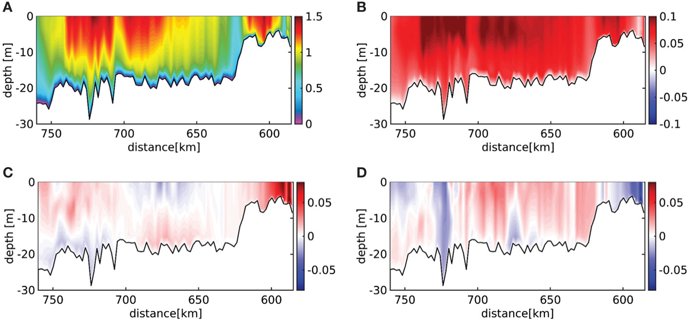
Figure 11 (A) Ensemble-averaged and time-averaged horizontal velocity current magnitude [m s^-1], (B) the ensemble-averaged annual change of current velocity magnitude [m s^-1 y^-1], (C) the difference in velocity magnitude between the upper-end and lower-end ensemble runs [m s^-1], (D) the difference in velocity magnitude between fast and slow rates of MSL rise [m s^-1] (see Figure 2B) along the Elbe estuary main (northern) channel during 2090–2099.

FIGURE 12

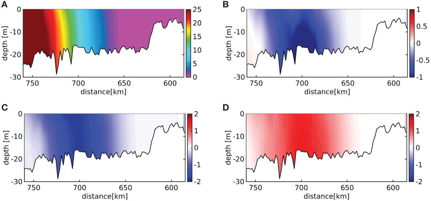
Figure 12 (A) Ensemble-averaged and time-averaged salinity [g kg^-1], (B) the ensemble-averaged annual change of salinity [g kg^-1 y^-1], (C) the difference in salinity concentration between the upper-end and lower-end ensemble runs [g kg^-1], (D) the difference in salinity concentration [g kg^-1] between fast and slow rates of mean sea-level rise (see Figure 2B) along the Elbe estuary main (northern) channel during 2090–2099.

Freshening in the lower estuary between km 670 and km 740 reveals increasing river discharge (Figures 8H, 12B and Supplementary Material Table 1) that tend to locally cancel out estuarine circulation (Supplementary Figure S5B). The pattern of reducing salinity in the lower estuary is repeated by the ensemble spread of salinity, i.e. the difference between the lower-end and upper-end ensemble members with the latter featuring 187 m³ s^-1 higher discharge on average (Figure 12C and Supplementary material Table 1). The corresponding ensemble spread of current magnitudes reveal clear positive differences only close to the tidal weir, while, in middle reaches, near-surface flows even reduce in the upper-end realisation, i.e. in the 95th percentile ensemble run vs. the 5th percentile ensemble run (Figure 11C). This shows that, in the main estuarine water body, the dampening of the flood currents due to the higher river runoff outweighs the strengthening of the flood flow due to rising MSL. The spread pattern of current magnitude due to different rates of MSL rise demonstrates vertically sheared differences in the outer estuary up to km 725 indicative of changing baroclinic flows under the upper-end MSL trajectory (Figure 11D). From km 710 up to the beginning of the shallow, upper estuary differences are mostly positive. This identifies sea level rise as the main driver of a largely uniform increase in current velocity magnitude along the entire estuary, while factors related to internal variability, such as river discharge, lead to locally differing changes. A special case is residual flow, which can be amplified by both higher sea level and aspects of internal variability – such as differences in the flow regime (see spread patterns in Supplementary Figures S5C, D).

The response of turbulent diffusivities to the imposed MSL rise and regional climate simulations is similar to that of current velocities, demonstrating an almost uniform increase along the estuarine channel (Figures 12B, 13B). The trend is locally enhanced in the deepened middle reaches that also demonstrate the highest average turbulent diffusivities (Figures 13A, B). In the same area, ensemble spread reveals the largest positive differences (Figure 13C), which can be partly attributed to the retreat of the salinity front in the upper-end ensemble run (Figure 12B and Supplementary Material Table 1). The increase of freshwater input would also explain the reduction of diffusivities in mouth of the estuary downstream of km 720 that becomes the centre of the salinity front attenuating turbulence production (Figures 12B, C, 13B, C). Spread under different rates of MSL rise shows approximately the inverse pattern of ensemble spread of diffusivities (Figures 13D, C). This results from the amplification of the salinity intrusion under higher MSL leading to the damping of turbulence at the downstream end of the freshwater reach between km 630 and km 680 (Figures 2B, 13D, 12D). Outside this region, higher MSL is associated with enhanced turbulent diffusivities (Figure 13D). However, it is important to note that spread due to internal variability is locally a multiple of spread under different MSLs (Figures 13C, D). This means that mixing in the water column is locally largely controlled by internal variability, which, thus, maybe interpreted as a source of uncertainty. The conclusion is that the management of subsystems such as sediment dynamics and biology controlled by vertical mixing needs to take into account the variability inherent to ocean–atmosphere interactions.

FIGURE 13

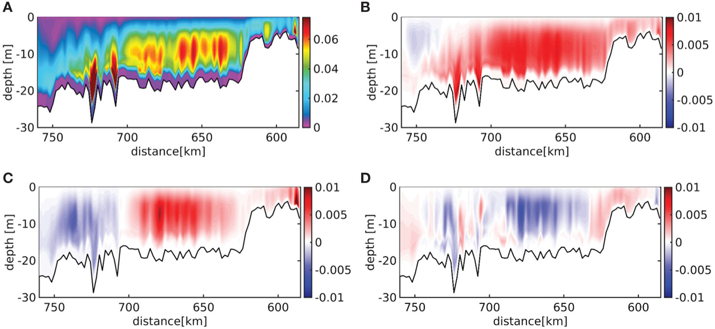
Figure 13 (A) Ensemble-averaged and time-averaged vertical eddy diffusivity [m² s^-1], (B) the ensemble-averaged annual change of eddy diffusivity [m² s^-1 y^-1], (C) the difference in eddy diffusivity between the upper-end and lower-end ensemble runs [m² s^-1], (D) the difference in eddy diffusivity concentration [m² s^-1] between fast and slow rates of mean sea-level rise (see Figure 2B) along the Elbe estuary main (northern) channel during 2090–2099.

4 Discussion

The ensemble simulations resulted in regionalised for the SNS estimates of MSL, MSL change and mean (change) of the M2 tidal amplitude during 2090–2099 that set the boundary conditions for the projected estuarine response that was presented with a focus on ensemble mean, ensemble spread and time evolution. In the Elbe estuary, the MWL rose upstream with the spread of ~0.5 m dominated by the extreme percentiles of MSL rise. The ensemble spread became important only in the shallow upper estuary, attaining 0.20 m at Bunthaus. The shallow upper reach also revealed a steep increase of MWLs towards the tidal weir. The along-channel profile of the M2 tidal amplitude was very similar to historic conditions, and the spread reached merely a couple of centimetres indicating the dominance of the bathymetric (frictional) control. The dynamical response of the M2 amplitude to the decadal trends of the MSL and M2 tidal amplitude was more pronounced showing an increase of ~7 mm y^-1 at the mouth and by ~14 mm y^-1 in the area of the port of Hamburg. In this area, the M2 tidal amplitude further demonstrated an opposite adjustment of its trend in comparison with the MWL. During the period of strong increase of the tidal amplitude, the MWL stagnated or even reduced while increasing quickly, when the rates of increase of the tidal amplitude attenuated. An increase in the tidal range that is compensated by decreasing MWLs has also been found as a result of the deepening of estuaries (e.g. Helaire et al., 2019) indicating that these two water level parameters should be considered in combination if no robust simulation of extreme events is available. Here, the hourly time resolution of the model output allowed a joint interpretation of average mean and average instantaneous extreme water levels that revealed both tides and the MWL as underlying drivers or predictors of the extreme water levels. Furthermore, the study also demonstrated considerable range of projected extreme water levels in the Elbe estuary, which was up to 0.57 m (Bunthaus), slightly exceeding the spread of MSL imposed at the open boundary. Ensemble spread was even larger reaching 0.58 m at the same station in the upper estuary. Still, the analysis of the seasonal mean and maxWLs revealed ranges of 0.6 and 1.95 m, respectively, at the Hamburg station emphasizing the pronounced seasonality of extreme events in this area. Absolute maxWLs with a median of 4.82 m occurred at the tidal weir, and synchronous extreme water levels were mainly recorded in the upper reach. The examination of the timing and magnitude of extreme water levels revealed a close relationship between monthly mean and monthly maxWLs in the shallow upper estuary. At the Bunthaus station, the correlation of monthly maximum and monthly MWLs weakened during the decadal simulations, reducing from R = 0.72 (2090–2094) to R = 0.56 (2095–2099). This location experienced a strong decadal increase of the M2 tidal amplitude and MWLs, respectively, and became affected by both storm and river surges. Monthly MWLs showed a moderate relationship of positive correlations with river discharge with R = 0.36 during 2090–2094 and R = 0.45 during 2095–2099, respectively. The positive correlation between river discharge and the M4 amplitude strengthened during the decadal simulations. The monthly maxWL was weakly anti-correlated with the monthly M2 tidal amplitude (R ~ -0.3), and the relationship slightly strengthened in the second half of the decade. This reveals an important insight because it clarifies that the tidal range is not a suitable predictor for extreme surges in this part of the estuary and potential adaptation measure cannot be assessed based on solely their ability to control the tidal range. The scatter of maximum monthly water levels over river discharge was large, and extreme surges happened at both low runoff below 500 m³ s^-1 and high runoff beyond 2,000 m³ s^-1. This result implicates that the management of river discharge, such as for example active weir control, could play a decisive role in mitigating extreme water levels in this region. Overall, the Bunthaus station appeared as a location responding to both climatic change from the sea and from the land side. This was evidenced, for example, by an increase of the spread of monthly maxWLs with MSL rise when ensemble spread, representing internal climate variability, became smaller.

In the water column, imposed decadal changes enhanced the average current velocity magnitude and turbulent diffusivities. MSL rise, represented by the spread between its projected 5th and 95th percentiles, increased salinity intrusion, while ensemble spread tended to reverse the salinity intrusion due to the high average freshwater discharge predicted by the upper-end ensemble run. The differences between lower- and higher-end ensemble runs also revealed opposite trends to the effects of MSL rise, showing the attenuation of horizontal velocities and turbulent diffusivities locally. The ensemble spread of turbulent diffusivities locally reached 0.01 m² s^-1 several times exceeding spread due to the projected MSL that reached approximately 0.0025 m² s^-1. This result demonstrates that the impact of the internal variability of the ocean–atmosphere system on vertical mixing (and related along-channel dispersion) may surpass the relevance of the spread of projected MSL and underlying climate uncertainty. Furthermore, the finding indicates that the transient evolution of sub-systems like sediment dynamics and ecology that are controlled by vertical mixing may be dominantly affected by internal variability on the decadal timescale. The conclusion is that the projections of estuarine hydrodynamics and even more so the coupled modelling and design of adaptation measures should not ignore the potential effects of internal variability.

This study contributes to the developing literature on regional climate projections that investigate the response of semi-enclosed basins and connected estuaries to the aspects of climatic change. The originality of this work consists of the combination of dynamical MSL and RCM simulations for the forcing of the shelf and estuary dynamics in a consistent future scenario focusing on mean states, trends and projected ranges relating to the type of climatic forcing. The approach is different from the studies that apply a fix increment of MSL change at the open boundary to compare simulations with and without the fix increment, respectively (Jiang et al., 2020; Feizabadi et al., 2022). It is also different from studies accomplishing a dynamical downscaling by applying forcing time series condensed from a much-longer simulation period (of a GCM or RCM), potentially blurring inter-annual, seasonal and short-scale variability (e.g. Khangaonkar et al., 2019). The advantage of our approach is that relevant bandwidths of water level parameters and other hydrodynamic parameters can be derived in a dynamically consistent manner for future-oriented planning while keeping the full dynamical information from tidal to decadal time scales. Simplified approaches that are still frequently used neglect e.g. correlations between sea level rise and decadal changes, which means that possible amplifications or compensations are not recorded. Due to the simulation time of 10 years, however, the present model study cannot be used to assess climate change in the proper sense, even though the selection of ensemble members from the regional climate simulations allows a fairly robust estimation of decadal change under the conditions of intensive climatic change. For a conclusive quantification of estuarine climate change, longer simulation times are necessary, covering as a minimum one nodal tide period for a historic and future time slice.

In comparison with climate change literature, our work demonstrated good agreement with previous works that studied the estuarine or shelf sea dynamics of climatic change from a different viewpoint. This regards, for example, the effect of several decimetres of increase of MSL on M2 tides in the SNS where numerical simulations produced a change pattern and a magnitude of change very similar to Schindelegger et al. (2018) in the central and south-western North Sea or Rasquin et al. (2020) in the German Bight. In the area of the Elbe estuary, the isolated effect of a higher MSL was enhancing the salinity intrusion, which conforms, for example, with the results of Feizabadi et al. (2022) simulating the impact of sea level rise on the Hudson–Raritan estuary. Downscaling the effect of a fix increment of MSL change to the Elbe estuary, Rasquin et al. (2020) reported that 0.8 m of MSL rise leads to an increase of the M2 tidal amplitude by a couple of centimetres in the middle reaches and up to 10 cm in area of the port of Hamburg. Studying the difference between tides forced by the 5th and 95th percentiles of projected MSL rise, we came to a similar conclusion showing that the spread resulting from using the different rates of global MSL rise was no larger than a couple of centimetres. The response to dynamical sea level rise in combination with the tidal forcing by the RCM was more pronounced revealing a ~ 10 cm/decade increase of the M2 tidal amplitude during the decadal MSL rise of 0.12 m. A likely explanation is that, firstly, the coupling of vertical and horizontal tides with RCM output at the open boundary more completely defines propagating into model area tides under RCP8.5 than other methods like the use of a tidal model, including the nodal tide that is not output by standard tidal models (e.g. Lyard et al., 2021). Secondly, progressive decadal climatic change in the RCM correlates with progressing MSL rise leading to higher inputs of momentum into the child model at the open boundary. These are the natural advantages of the dynamical downscaling of the original GCM/RCM simulations in comparison to experimental set-ups where historic forcing data are enhanced by some constant increment of MSL and/or salinity, temperature etc. In the estuary, the effects of dynamical coupling at the open boundary get further amplified by channel convergence and buoyancy gradient, which was demonstrated in this work by increasing the magnitude and range of projected monthly extreme water levels.

The results of this study are representative for estuaries in the area of the northwestern shelf of the Atlantic region with similar geometric characteristics including channel convergence and a shallow upper reach and that are subject to similar environmental conditions like river discharge. Typical candidates would be the meso- to macro-tidal systems like the Scheldt estuary, the Ems estuary and the Loire estuary (see Winterwerp et al., 2013). In these systems, strong tidal forcing poses an adaptation pressure to vigorous water movements, which means that the banks along these estuaries are usually well protected increasing, however, the coastal squeeze and convergence of the estuarine geometry. This may cause the amplification of extreme events when a surge is confined by dikes close to the river bed eventually exerting high pressure on the coastal defences. For this reason, it is important to know the range of water level parameters due to internal variability and underlying climatic variations in order to provide reliable information for the long-term development of the estuarine space. Although these are system specific, we have shown here that they do matter in an estuary of moderate length and depth and subject to moderate mean river discharge.

In this exercise, the bathymetry was assumed to be constant, which is a reasonable assumption for a managed system like the Elbe estuary. Without the permanent maintenance dredging, the region of the port of Hamburg would silt up at high rates, inevitably changing resonance characteristics, tidal currents and estuarine water levels. Future studies taking into account further climate feedbacks, including socio-economic ones, might argue that the regional policy will adapt to climatic change and its consequences by refraining from ecologically and economically costly maintenance dredging. Such a study design would require taking into account morphodynamic feedbacks that occur in meso- and macro-tidal systems (Figueroa et al., 2022). Significant morphodynamic changes are to be expected in the German Bight and the Wadden Sea, especially over longer periods of time. However, there is no indication that these will principally alter the tidal forcing of the Elbe estuary. In this respect, Supplementary Figure S3A gives an example of the shift of the inter-tidal zone from a historical simulation period (1997–2006) to the timeslice covered by the simulations shown in this study (2090–2099). The figure highlights that historical high waters are confined by an abrupt steepening of the bathymetry while future high waters meet a flattening bathymetry. The “kink” overcome by the rising tide during late flood phase in the future simulations could, in reality, be modified by the accretion of sediments in the non-managed Wadden Sea, re-establishing the steeper wall confining historical rising tides. However, it is beyond the scope of this study to address the morphodynamic response in the German Bight during the decadal simulations. In a follow-up study, we plan to investigate the estuarine morphodynamic responses to climate change and human interventions such as adaptation measures in more detail.

5 Conclusions

This study presented a modelling framework to derive future estuarine dynamics based on global and regional climate projections using the SCHISM unstructured numerical modelling software. Illustrating the practical utility of the framework, decadal MSL change and regional climate variability were downscaled to the Elbe estuary. The analysis of the results focused on temporal and spatial scales of sea level variability and on the projected spread, its time evolution and spatial patterns. Decadal MSL change and regional climatic change, represented by regionalised global MSL projections and a subset of RCM ensemble simulations, respectively, induced a pronounced estuarine response demonstrating the particular sensitivity of estuarine hydrodynamics to the applied forcing. The sensitivity was evidenced by 1) upstream rising MWLs inside the estuary (Cuxhaven: 0.91 m, Hamburg: 1.10 m), 2) upstream increasing amplification of extreme water levels (Cuxhaven: 3.22 m, Hamburg: 4.07 m), 3) a wide range of extreme water levels under the applied high-emission scenario of ~0.55 m, 4) high rates of increase of MWLs (Cuxhaven: 19.7 mm y^-1, Hamburg: 21.1 mm y^-1) and 5) increasing extreme water levels (Cuxhaven: 16.0 mm y^-1 and Hamburg: 17.9 mm y^-1). These rates constitute a multiple of currently observed MSL change, which currently equals 1.8 mm y^-1 at Cuxhaven at the mouth of the estuary. The dynamic downscaling exercise also revealed crucial information for the understanding and management of the estuary transient trends such as the non-linear response of the MWL and M2 tidal amplitude to the applied decadal climatic forcing in the area of the transition between the deepened freshwater reach and the shallow upper estuary. This involved MWLs reducing locally while the tidal amplitude increased steeply in the same area. Moreover, in the shallow upper estuary, decadal climatic change and long-period tidal forcing impacted on the relationships of the M2 tidal amplitude to the mean monthly water level and maximum monthly water level to the mean monthly water level. Regardless of the estuarine response to marine forcing, river discharge demonstrated stable positive feedback on monthly MWLs in the shallow upper estuary. MSL rise and internal variability, represented by the global projections and RCM ensemble spread, respectively, also affected dynamics in the water column stimulating partially opposing trends. During the decadal MSL rise, current magnitude and turbulent diffusivities increased throughout the estuary. Internal variability, via different trajectories of average water levels, wind speed and river discharge, partially led to opposite effects, reducing currents and mixing locally.

The study highlighted the range and potential inter-annual-to-decadal trends of the estuarine response to forced climatic changes that impacted both the water surface variability and processes in the water column. It became clear that future sustainable estuarine management must take into account many interrelated aspects of hydrodynamics. For example, adaptation studies envisioning future extreme water levels (but that cannot resolve the necessary scales) must account for changes in both the MWL and tidal range. In the shallow upper estuary, these two variables showed spatially varying compensating trends but with different ranges of variability. As both have been shown to be responsible for changes in extreme water levels, with clear trends in response to sea level rise, a key conclusion is that adaptation measures to control extreme water levels must start at the estuarine geometry below the MWL. Only if the maladaptations that made the upper estuary susceptible to extreme floods can be identified will it be possible to responsibly design measures such as increasing inter-tidal areas and removing narrow coastal defences. Our results show that a focus on the reduction of the tidal amplitude alone is not sufficient to tackle the mitigation of extreme water levels. The response of turbulent diffusivities to climatic forcing showed locally different trends due to a higher MWL and internal variability. Overall, considered herein decadal climatic change enhanced vertical mixing suggesting far-reaching effects on dependent variables such as turbidity. To substantiate this thesis, it is necessary to perform coupled simulations under a similar scenario, which will be the subject of a follow-up study. It is also important to extend the simulation period as far as possible in order to achieve a robust quantification of local climate change through the consistent application of numerical downscaling.

Data availability statement

The raw data supporting the conclusions of this article will be made available by the authors, without undue reservation.

Author contributions

JP generated the data set, performed the data analysis and wrote the first manuscript draft. BM and MP provided model boundary conditions. JS and CS advised on the numerical modelling and data analysis. All authors contributed to the article and approved the submitted version.

Funding

This project is a contribution to theme “C3: Sustainable Adaption Scenarios for Coastal Systems” of the Cluster of Excellence EXC 2037 ‘CLICCS - Climate, Climatic Change, and Society’ – Project Number: 390683824 funded by the Deutsche Forschungsgemeinschaft (DFG, German Research Foundation) under Germany’s Excellence Strategy. This contribution was funded by the Helmholtz-Gemeinschaft Deutscher Forschungszentren (HGF) in the framework of the CLICCS-HGF networking project. JP acknowledges funding from the BMBF in the framework of the KÜNO project “Blue Estuaries”(FKZ 03V01565). MP was supported by the Met Office Hadley Centre Climate Programme funded by BEIS. JS acknowledges EU Green Deal Project REST-COAST “Large scale restoration of coastal ecosystems through rivers to sea connectivity” (Grant Agreement 101037097).

Acknowledgments

We are grateful to Dr. Moritz Mathis and Dr. Ralf Weisse (both Hereon) and Dr. Thomas Pohlmann (University of Hamburg) for fruitful discussions. Further, we thank the teams of DKRZ, Hereon and Juelich clusters for their technical support and advice.

Conflict of interest

The authors declare that the research was conducted in the absence of any commercial or financial relationships that could be construed as a potential conflict of interest.

Publisher’s note

All claims expressed in this article are solely those of the authors and do not necessarily represent those of their affiliated organizations, or those of the publisher, the editors and the reviewers. Any product that may be evaluated in this article, or claim that may be made by its manufacturer, is not guaranteed or endorsed by the publisher.

Supplementary material

The Supplementary Material for this article can be found online at: https://www.frontiersin.org/articles/10.3389/fmars.2023.1102485/full#supplementary-material

Footnotes

1. ^ https://meeresspiegel-monitor.de/cuxhaven/trend/index.php.de.
2. ^ Herr der Flut. In: Der Spiegel. Nr. 10, 1962, S. 26 (https://www.spiegel.de/politik/herr-der-flut-a-db48b7a5-0002-0001-0000-000032655070).

References

Arns A., Dangendorf S., Jensen J., Talke S., Bender J., Pattiaratchi C. (2017). Sea-Level rise induced amplification of coastal protection design heights. Sci. Rep. 7 (1), 1–9. doi: 10.1038/srep40171

PubMed Abstract | CrossRef Full Text | Google Scholar

Church J. A., Clark P. U., Cazenave A., Gregory J. M., Jevrejeva S., Levermann A., et al. (2013). “'Sea level change',” in Climate change 2013: The physical science basis. contribution of working group I to the fifth assessment report of the intergovernmental panel on climate change. Eds. Stocker T. F., Qin D., Plattner G.-K. (Cambridge; New York: Cambridge University Press), 1137–1216. Available at: http://www.climatechange2013.org/images/report/WG1AR5_Chapter13_FINAL.pdf.

Google Scholar

Codiga D. L. (2011). “Unified tidal analysis and prediction using the UTide Matlab functions. technical report 2011-01,” in Graduate school of oceanography (Narragansett, RI: University of Rhode Island), 59pp. doi: 10.13140/RG.2.1.3761.2008

CrossRef Full Text | Google Scholar

Collins M. ,. R., Knutti J., Arblaster J.-L., Dufresne T., Fichefet P., Friedlingstein X., et al. (2013). “Long-term climate change: Projections, commitments and irreversibility,” in Climate change 2013: The physical science basis. contribution of working group I to the fifth assessment report of the intergovernmental panel on climate change. Eds. Stocker T. F. D., Qin G.-K., Plattner M., Tignor S. K., Allen J., Boschung A., Nauels Y., Xia V. (Cambridge, United Kingdom and New York, NY, USA: Cambridge University Press).

Google Scholar

Dangendorf S., Mudersbach C., Wahl T., Jensen J. (2013b). Characteristics of intra-, inter-annual and decadal sea-level variability and the role of meteorological forcing: the long record of Cuxhaven. Ocean Dynamics 63, 209–224. doi: 10.1007/s10236-013-0598-0

CrossRef Full Text | Google Scholar

Dangendorf S., Wahl T., Mudersbach C., Jensen J. (2013a). “The seasonal mean Sea level cycle in the southeastern north Sea,” [in special issue: International Coastal Symposium Volume 2] Journal of Coastal Research, 65, 1915–1920. doi: 10.2112/SI65-324.1

CrossRef Full Text | Google Scholar

Elizalde A., Groeger M., Mathis M., Mikolajewicz U., Bülow K., Hüttl-Kabus S., et al. (2014). MPIOM-REMO a coupled regional model for the north Sea. KLIWAS Schriftenreihe, Bundesanstalt für Gewässerkunde, Koblenz, Germany, 58/2014. doi: 10.5675/Kliwas_58/2014_MPIOM-REMO

CrossRef Full Text | Google Scholar

Eyring V., Bony S., Meehl G. A., Senior C. A., Stevens B., Stouffer R. J., et al. (2016). Overview of the coupled model intercomparison project phase 6 (CMIP6) experimental design and organization. Geoscientific Model. Dev. 9 (5), 1937–1958. doi: 10.5194/gmd-9-1937-2016

CrossRef Full Text | Google Scholar

Feizabadi S., Rafati Y., Ghodsian M., Akbar Salehi Neyshabouri A., Abdolahpour M., Mazyak A. R. (2022). Potential sea-level rise effects on the hydrodynamics and transport processes in Hudson–raritan estuary, NY–NJ. Ocean Dynamics 72 (6), 421–442. doi: 10.1007/s10236-022-01512-0

CrossRef Full Text | Google Scholar

Ferrero B., Tonelli M., Marcello F., Wainer I. (2021). Long-term regional dynamic sea level changes from CMIP6 projections. Adv. Atmospheric Sci. 38 (2), 157–167. doi: 10.1007/s00376-020-0178-4

CrossRef Full Text | Google Scholar

Figueroa S. M., Son M., Lee G. H. (2022). Effect of estuarine dam location and discharge interval on estuarine hydrodynamics, sediment dynamics, and morphodynamics. Front. Mar. Sci. 9, 2168. doi: 10.3389/fmars.2022.1035501

CrossRef Full Text | Google Scholar

Fox-Kemper B., Hewitt H. T., Xiao C., Aðalgeirsdóttir G., Drijfhout S. S., Edwards T. L., et al. (2021). “Ocean, cryosphere and Sea level change,” in Climate change 2021: The physical science basis. contribution of working group I to the sixth assessment report of the intergovernmental panel on climate change. Eds. Masson-Delmotte V. ,. P., Zhai A., Pirani S. L., Connors C., Péan S., Berger N., Caud Y., Chen L., Goldfarb M. I., Gomis M., Huang K., Leitzell E., Lonnoy J. B. R. (Cambridge, United Kingdom and New York, NY, USA: Cambridge University Press), 1211–1362. doi: 10.1017/9781009157896.011

CrossRef Full Text | Google Scholar

Golledge N. R. (2020). Long-term projections of sea-level rise from ice sheets. Wiley Interdiscip. Reviews: Climate Change 11 (2), e634. doi: 10.1002/wcc.634

CrossRef Full Text | Google Scholar

Hausfather Z., Peters G. P. (2020). Emissions - the 'business as usual' story is misleading. Nature 577 (7792), 618–620. doi: 10.1038/d41586-020-00177-3

PubMed Abstract | CrossRef Full Text | Google Scholar

Hein S. S., Sohrt V., Nehlsen E., Strotmann T., Fröhle P. (2021). Tidal oscillation and resonance in semi-closed estuaries–empirical analyses from the Elbe estuary, north Sea. Water 13 (6), 848. doi: 10.3390/w13060848

CrossRef Full Text | Google Scholar

Helaire L. T., Talke S. A., Jay D. A., Mahedy D. (2019). Historical changes in lower Columbia river and estuary floods: A numerical study. J. Geophysical Research: Oceans 124 (11), 7926–7946. doi: 10.1029/2019JC015055

CrossRef Full Text | Google Scholar

Hermans T. H., Tinker J., Palmer M. D., Katsman C. A., Vermeersen B. L., Slangen A. (2020). Improving sea-level projections on the northwestern European shelf using dynamical downscaling. Climate Dynamics 54 (3), 1987–2011. doi: 10.1007/s00382-019-05104-5

CrossRef Full Text | Google Scholar

Huang W., Zhang Y. J., Wang Z., Ye F., Moghimi S., Myers E., et al. (2022). Tidal simulation revisited. Ocean Dynamics 72 (3), 187–205. doi: 10.1007/s10236-022-01498-9

CrossRef Full Text | Google Scholar

IPCC (2021). “Summary for policymakers,” in Climate change 2021: The physical science basis. contribution of working group I to the sixth assessment report of the intergovernmental panel on climate change. Eds. Masson-Delmotte V. ,. P., Zhai A., Pirani S. L., Connors C., Péan S., Berger N. (Cambridge, United Kingdom and New York, NY, USA: Cambridge University Press), 3–32. doi: 10.1017/9781009157896.001

CrossRef Full Text | Google Scholar

Jackson L. P., Jevrejeva S. (2016). A probabilistic approach to 21st century regional sea-level projections using RCP and upper-end scenarios. Global Planetary Change 146, 179–189. doi: 10.1016/j.gloplacha.2016.10.006

CrossRef Full Text | Google Scholar

Jiang L., Gerkema T., Idier D., Slangen A., Soetaert K. (2020). Effects of sea-level rise on tides and sediment dynamics in a Dutch tidal bay. Ocean Sci. 16 (2), 307–321. doi: 10.5194/os-16-307-2020

CrossRef Full Text | Google Scholar

Jones J. E., Davies A. M. (2008). On the modification of tides in shallow water regions by wind effects. J. Geophysical Research: Oceans 113, C05014. doi: 10.1029/2007JC004310

CrossRef Full Text | Google Scholar

Kerner M. (2007). Effects of deepening the Elbe estuary on sediment regime and water quality. Estuarine Coast. shelf Sci. 75 (4), 492–500. doi: 10.1016/j.ecss.2007.05.033

CrossRef Full Text | Google Scholar

Khangaonkar T., Nugraha A., Xu W., Balaguru K. (2019). Salish Sea response to global climate change, sea level rise, and future nutrient loads. J. Geophysical Research: Oceans 124 (6), 3876–3904. doi: 10.1029/2018JC014670

CrossRef Full Text | Google Scholar

Khojasteh D., Glamore W., Heimhuber V., Felder S. (2021). Sea Level rise impacts on estuarine dynamics: A review. Sci. Total Environ. 780, 146470. doi: 10.1016/j.scitotenv.2021.146470

PubMed Abstract | CrossRef Full Text | Google Scholar

Kopp R. E., Horton R. M., Little C. M., Mitrovica J. X., Oppenheimer M., Rasmussen D. J., et al. (2014). Probabilistic 21st and 22nd century sea-level projections at a global network of tide-gauge sites. Earth's Future 2, 383–406. doi: 10.1002/2014EF000239

CrossRef Full Text | Google Scholar

Lang A., Mikolajewicz U. (2020). Rising extreme sea levels in the German bight under enhanced CO2 levels: A regionalised large ensemble approach for the north Sea. Clim Dyn 55, 1829–1842. doi: 10.1007/s00382-020-05357-5

CrossRef Full Text | Google Scholar

Lyard F. H., Allain D. J., Cancet M., Carrère L., Picot N. (2021). FES2014 global ocean tide atlas: design and performance. Ocean Sci. 17 (3), 615–649. doi: 10.5194/os-17-615-2021

CrossRef Full Text | Google Scholar

Lyu K., Zhang X., Church J. A. (2020). Regional dynamic sea level simulated in the CMIP5 and CMIP6 models: Mean biases, future projections, and their linkages. J. Climate 33 (15), 6377–6398. doi: 10.1175/JCLI-D-19-1029.1

CrossRef Full Text | Google Scholar

Maher N., Lehner F., Marotzke J. (2020). Quantifying the role of internal variability in the temperature we expect to observe in the coming decades. Environ. Res. Lett. 15 (5), 054014. doi: 10.1088/1748-9326/ab7d02

CrossRef Full Text | Google Scholar

Mathis M., Elizalde A., Mikolajewicz U., Pohlmann T. (2015). Variability patterns of the general circulation and sea water temperature in the north Sea. Prog. Oceanography 135, 91–112. doi: 10.1016/j.pocean.2015.04.009

CrossRef Full Text | Google Scholar

Mathis M., Mikolajewicz U. (2020). The impact of meltwater discharge from the Greenland ice sheet on the Atlantic nutrient supply to the northwest European shelf. Ocean Sci. 16 (1), 167–193. doi: 10.5194/os-16-167-2020

CrossRef Full Text | Google Scholar

Mayer B., Mathis M., Mikolajewicz U., Pohlmann T. (2022a). RCP8.5-projected changes in German Bight storm surge characteristics from regionalized ensemble simulations for the end of the twenty-first century. Frontiers in Climate, 4, 1-18, 25 November 2022, Sec. Predictions and Projections. doi: 10.3389/fclim.2022.992119

CrossRef Full Text | Google Scholar

Mayer B., Mathis M., Pohlmann T. (2022b). Effects of climate change on extreme sea levels in the North Sea (ECCES): Regionalized MPIOM-REMO climate ensemble. World Data Center for Climate (WDCC) at DKRZ. doi: 10.26050/WDCC/ECCES_MPIOM-REMO

CrossRef Full Text | Google Scholar

Meinshausen M., Smith S. J., Calvin K., Daniel J. S., Kainuma M. L.T., Lamarque J-F., et al. (2011). The RCP greenhouse gas concentrations and their extensions from 1765 to 2300. Climatic Change 109, 213. doi: 10.1007/s10584-011-0156-z

CrossRef Full Text | Google Scholar

Mikolajewicz U., Sein D. V., Jacob D., Königk T., Podzun R., Semmler T. (2005). Simulating Arctic sea ice variability with a coupled regional atmosphere-ocean-sea ice model. Meteorologische Z. 14 (6), 793–800. doi: 10.1127/0941-2948/2005/0083

CrossRef Full Text | Google Scholar

Palmer M. D., Gregory J. M., Bagge M., Calvert D., Hagedoorn J. M., Howard T., et al. (2020). Exploring the drivers of global and local sea-level change over the 21st century and beyond. Earth's Future 8, e2019EF001413. doi: 10.1029/2019EF001413

CrossRef Full Text | Google Scholar

Palmer M., Howard T., Tinker J., Lowe J., Bricheno L., Calvert D., et al. (2018). UKCP18 marine report. Met Office Hadley Centre, Exeter, United Kingdom, 133pp.

Google Scholar

Pein J., Eisele A., Sanders T., Daewel U., Stanev E. V., Van Beusekom J. E., et al. (2021). Seasonal stratification and biogeochemical turnover in the freshwater reach of a partially mixed dredged estuary. Front. Mar. Sci. 8. doi: 10.3389/fmars.2021.623714

CrossRef Full Text | Google Scholar

Pelling H. E., Green J. M. (2014). Impact of flood defences and sea-level rise on the European shelf tidal regime. Continental Shelf Res. 85, 96–105. doi: 10.1016/j.csr.2014.04.011

CrossRef Full Text | Google Scholar

Rasquin C., Seiffert R., Wachler B., Winkel N. (2020). The significance of coastal bathymetry representation for modelling the tidal response to mean sea level rise in the German bight. Ocean Sci. 16, 31–44. doi: 10.5194/os-16-31-2020

CrossRef Full Text | Google Scholar

Rohde H. (1971). “Eine studie über die entwicklung der Elbe als schiffahrtsstrasse (in german). Dissertation,” in Mitteilungen des franzius-instituts für grund- und wasserbau der technischen universität hannover (Hannover, Germany: University of Hannover), vol. 36.1971.

Google Scholar

Schindelegger M., Green J. A. M., Wilmes S. B., Haigh I. D. (2018). Can we model the effect of observed sea level rise on tides? J. Geophysical Research: Oceans 123 (7), 4593–4609. doi: 10.1029/2018JC013959

CrossRef Full Text | Google Scholar

Sohrt V., Hein S. S., Nehlsen E., Strotmann T., Fröhle P. (2021). Model based assessment of the reflection behavior of tidal waves at bathymetric changes in estuaries. Water 13 (4), 489. doi: 10.3390/w13040489

CrossRef Full Text | Google Scholar

Stanev E. V., Jacob B., Pein J. (2019). German Bight estuaries: An inter-comparison on the basis of numerical modeling. Continental Shelf Res. 174, 48–65. doi: 10.1016/j.csr.2019.01.001

CrossRef Full Text | Google Scholar

Stanev E. V., Ricker M. (2020). Interactions between barotropic tides and mesoscale processes in deep ocean and shelf regions. Ocean Dynamics 70, 713–728. doi: 10.1007/s10236-020-01348-6

CrossRef Full Text | Google Scholar

Sterr H. (2008). Assessment of vulnerability and adaptation to sea-level rise for the coastal zone of Germany. J. Coast. Res. 24 (2), 380–393. doi: 10.2112/07A-0011.1

CrossRef Full Text | Google Scholar

Taylor K. E., Stouffer R. J., Meehl G. A. (2012). An overview of CMIP5 and the experiment design. Bull. Am. meteorological Soc. 93 (4), 485–498. doi: 10.1175/BAMS-D-11-00094.1

CrossRef Full Text | Google Scholar

Weeks J. H., Fung F., Harrison B. J., Palmer M. D. (2023). The evolution of UK sea-level projections. Environ. Res. Commun. in press. doi: 10.1088/2515-7620/acc020

CrossRef Full Text | Google Scholar

Weilbeer H. (2014). Sediment transport and sediment management in the Elbe estuary (in German). Die Küste 81 Model. 81), 409–426. Available at: https://hdl.handle.net/20.500.11970/101703.

Google Scholar

Weilbeer H., Winterscheid A., Strotmann T., Entelmann I., Shaikh S., Vaessen B. (2021). “Analyse der hydrologischen und morphologischen entwicklung in der tideelbe für den zeitraum von 2013 bis 2018 (in German),” in Die Küste Karlsruhe, Germany: Bundesanstalt für wasserbau 89, 57–129. doi: 10.18171/1.089104

CrossRef Full Text | Google Scholar

Winterwerp J. C., Wang Z. B., van Braeckel A., van Holland G., Kösters F. (2013). Man-induced regime shifts in small estuaries–II: A comparison of rivers. Ocean Dynamics 63, 1293–1306. doi: 10.1007/s10236-013-0663-8

CrossRef Full Text | Google Scholar

Ye F., Zhang Y. J., Yu H., Sun W., Moghimi S., Myers E., et al. (2020). Simulating storm surge and compound flooding events with a creek-to-ocean model: Importance of baroclinic effects. Ocean Model. 145, 101526. doi: 10.1016/j.ocemod.2019.101526

CrossRef Full Text | Google Scholar

Zhang Y. J., Ye F., Stanev E. V., Grashorn S. (2016). Seamless cross-scale modeling with SCHISM. Ocean Model. 102, 64–81. doi: 10.1016/j.ocemod.2016.05.002

CrossRef Full Text | Google Scholar