Abstract
In this study, the effects of fully coupling the atmosphere, waves, and ocean compared with two-way-coupled simulations of either atmosphere and waves or atmosphere and ocean are analyzed. Two-year-long simulations (2017 and 2018) are conducted using the atmosphere–ocean–wave (AOW) coupled system consisting of the atmosphere model CCLM, the wave model WAM, and the ocean model NEMO. Furthermore, simulations with either CCLM and WAM or CCLM and NEMO are done in order to estimate the impacts of including waves or the ocean into the system. For the North Sea area, it is assessed whether the influence of the coupling of waves and ocean on the atmosphere varies throughout the year and whether the waves or the ocean have the dominant effect on the atmospheric model. It is found that the effects of adding the waves into the system already consisting of atmosphere and ocean model or adding the ocean to the system of atmosphere and wave model vary throughout the year. Which component has a dominant effect and whether the effects enhance or diminish each other depends on the season and variable considered. For the wind speed, during the storm season, adding the waves has the dominant effect on the atmosphere, whereas during summer, adding the ocean has a larger impact. In summer, the waves and the ocean have similar influences on mean sea level pressure (MSLP). However, during the winter months, they have the opposite effect. For the air temperature at 2 m height (T_2m), adding the ocean impacts the atmosphere all year around, whereas adding the waves mainly influences the atmosphere during summer. This influence, however, is not a straight feedback by the waves to the atmosphere, but the waves affect the ocean surface temperature, which then also feedbacks to the atmosphere. Therefore, in this study we identified a season where the atmosphere is affected by the interaction between the waves and the ocean. Hence, in the AOW-coupled simulation with all three components involved, processes can be represented that uncoupled models or model systems consisting of only two models cannot depict.
1 Introduction
The coupling between the atmospheric model and the ocean model is already commonly used to better describe the air–sea interaction at the interface of the two earth system components. By coupling the two models, the processes at the interface of the models can be explicitly simulated instead of being prescribed, parametrized, or even neglected, which in turn increases the models degrees of freedom (Gröger et al., 2021). Due to this interactive exchange of atmosphere and ocean parameters, the skill of the atmospheric model can be enhanced (Van Pham et al., 2014; Ho-Hagemann et al., 2015; Ho-Hagemann et al., 2017; Van Pham et al., 2018; Kelemen et al., 2019). Van Pham et al. (2014) showed an improvement of simulating the 2-m air temperature in a coupled system consisting of COSMO-CLM (CCLM) and NEMO compared with a stand-alone simulation of CCLM. In areas that are strongly influenced by the North and Baltic Sea (i.e., downwind of those regions), this improvement is more pronounced. In addition, Van Pham et al. (2018) illustrated that in decadal forecasts the predictive skill in 2-m air temperature is enhanced in the coupled system compared with the uncoupled system. In century-long simulations, Kelemen et al. (2019) found that the precipitation is even more influenced by the coupling of CCLM to NEMO than the 2-m air temperature. Ho-Hagemann et al. (2015, 2017) indicated that the coupled model COSTRICE improved the low-level large-scale moisture convergence over the North Atlantic and the moisture transport toward Central Europe. As a result, the simulated summer heavy rainfall improved compared with the stand-alone atmospheric model CCLM. For a specific storm event in the North Sea area, Ho-Hagemann et al. (2020) showed that the coupled system outperforms the stand-alone atmospheric model, especially by reducing the internal model variability in the coupled ensemble compared with the uncoupled ensemble.
Since ocean surface waves, hereafter called waves, are right at the interface of the atmosphere and the ocean, they determine the exchange of energy, heat, mass, and momentum between the two media (Cavaleri et al., 2012; Staneva et al., 2014). Previous studies have already shown that the waves impact the atmosphere (e.g., Wahle et al., 2017; Wiese et al., 2019; Wiese et al., 2020), as well as the ocean (e.g., Alari et al., 2016; Staneva et al., 2017; Bonaduce et al., 2020; Staneva et al., 2021).
In an atmosphere-only model, the roughness length of the ocean surface can be parameterized based on wind speed near the ground. When using a coupled atmosphere–wave model, the roughness length is calculated from wave parameters and is then passed to the atmospheric model. This feedback significantly influences the atmospheric model results, leading to a reduction in wind speed and a better agreement with observations, especially during extreme events (Wahle et al., 2017; Wiese et al., 2019; Wiese et al., 2020) but also during 1-year-long simulations (Varlas et al., 2020). Furthermore, the uncertainty of the atmospheric model can be reduced when coupling the two models (Wiese et al., 2020). In addition, the coupling of the wave model to the ocean model enhances the skill of the ocean model, especially during storm events (Staneva et al., 2017; Staneva et al., 2021). In the coupled model, the wave model gives the ocean model the Stokes–Coriolis forcing, as well as the momentum and energy fluxes depending on the current sea-state. In return, the ocean model sends the wave model a better estimate of the sea level. This coupling, on the one hand, affects the sea level estimate of the ocean model, especially during storm surge events, leading to a better agreement with observations (Staneva et al., 2017). On the other hand, the coupling of the wave model to the ocean model leads to changes in sea surface temperature (SST). Breivik et al. (2015) as well as Alari et al. (2016) found a warming in SST in the summer months in the extratropical region and the Baltic Sea, respectively. They showed that the mixing of the upper ocean is smaller when the wave model WAM is coupled to the ocean model NEMO, which they attributed to NEMO overdoing the mixing in the stand-alone standard setup.
Still, wave models are only rarely incorporated into coupled earth system models (Cavaleri et al., 2012; Schrum, 2017). However, some previous studies with model systems, consisting of atmosphere, wave, and ocean models, have already been carried out. They suggest that the inclusion of a wave model can be beneficial for the skill of all three models. Most of these studies, however, focus on short-term atmospheric events like hurricanes (Chen et al., 2007; Olabarrieta et al., 2012; Zambon et al., 2014; Pant and Prakash, 2020) or cold air outbreaks (Carniel et al., 2016). Wu et al. (2019) found a significant impact of the AOW coupling in the coastal areas in 2-month-long simulations (January and July 2015) due to the high-resolution model capturing coastal effects such as upwelling and their impact on the atmosphere. Recently, Gentile et al. (2021) investigated the sensitivity of extreme surface wind speeds to air–sea interactions in the Met Office’s UK Regional Coupled Environmental Prediction system consisting of atmosphere, waves, and ocean. They found an impact of coupling the ocean model to the atmospheric model on the SST. Also, they showed an impact of the inclusion of the wave model in the system already consisting of atmosphere and ocean on the wind speed, especially during extratropical cyclones. Furthermore, Gentile et al. (2022) used a convective-scale ensemble prediction system with dynamical atmosphere–ocean–wave coupling to simulate storm Ciara in February 2020 and showed that the coupling has a consistent impact across the 18 ensemble members. They hinted that the impacts of the coupling are comparable in size to that of adding perturbations to the initial conditions and lateral boundary conditions, as well as stochastic physics perturbations to the uncoupled atmosphere-only ensemble simulation, which implies that the coupling of ocean and wave to the atmosphere is an important aspect of model uncertainty.
Due to the results of the abovementioned studies, it can be expected that the effects of the wave model on the ocean model within the North and Baltic Sea can also affect the atmosphere. This can only become visible in a setup where all three models are coupled and exchange their parameters at the interface between the ocean and atmosphere through the waves. To evaluate those effects is the aim of the study presented here.
For that, we use the Geesthacht COAstal model SysTem (GCOAST) including the atmospheric model CCLM, the wave model WAM, and the ocean model NEMO. The aim of this study is to assess the impacts of the AOW coupling on the atmospheric model, especially the mean sea level pressure (MSLP), the 10-m wind speed (ff_10m), and the 2-m air temperature (T_2m). In simulations covering 2 years (2017 and 2018) with the AOW-coupled system as well as two-way coupling between atmosphere and waves or atmosphere and ocean, it is assessed whether the effects of the waves and the ocean on the atmosphere rather cancel each other out or enhance one another. Furthermore, it is investigated whether the influence of the coupling on the atmospheric model varies throughout the year and whether the inclusion of the waves or the ocean into the system has the dominant effect on the atmospheric model. Also, as mentioned above, since the direct influences of the waves and the ocean on the atmosphere are already studied with two-way-coupled simulations, we want to identify situations in which the atmospheric model is influenced by the feedback between the wave and the ocean model. Lastly, the results are compared with observations.
In the following, first, the models and observational data used in this study are presented (Section 2), which is followed by the introduction of the experimental setup for this study (Section 3). The results are presented in Sections 4, starting with the impacts on the monthly mean over the North Sea, followed by the evaluation of the indirect impacts of the wave model on the atmospheric model through the ocean model, and then a more in-depth analysis of two individual events and a comparison with observational data. The paper is warped up with Discussion and Conclusions in Section 5.
2 Numerical models and observations
2.1 Numerical models
In this study, numerical models for the atmosphere, ocean surface waves, and the ocean circulation are used. The atmospheric model utilized is the regional climate model of the COnsortium for Small-scale MOdeling (COSMO) in CLimate Mode (CLM) (CCLM) (Rockel et al., 2008; Doms and Baldauf, 2013). CCLM is the community model of the German regional climate research community. CCLM has already been used in previous studies, in a coupled mode to either a wave model (Wahle et al., 2017; Wiese et al., 2019; Li et al., 2020; Wiese et al., 2020; Li et al., 2021) or an ocean model (e.g., Van Pham et al., 2014; Ho-Hagemann et al., 2015; Ho-Hagemann et al., 2017; Will et al., 2017; Van Pham et al., 2018; Kelemen et al., 2019; Ho-Hagemann et al., 2020). CCLM is a non-hydrostatic limited area regional climate model. The primitive thermo-hydrodynamical equations describing a compressible flow in a moist atmosphere are solved on a rotated geographical Arakawa C grid using generalized terrain following height coordinates (Rockel et al., 2008; Doms and Baldauf, 2013). For the calculation of heat fluxes, CCLM uses the ‘TKE-based surface transfer scheme’. This study applied the CCLM version 5.0 with the coupling interface developed based on the unified OASIS interface of the CCLM version 4.8 (see Will et al., 2017).
For modelling the ocean surface waves, we applied the WAve Model WAM (WAMDI Group, 1988; ECMWF, 2019). This wave model has been used previously coupled to CCLM (Wahle et al., 2017; Wiese et al., 2019; Li et al., 2020; Wiese et al., 2020; Li et al., 2021), as well as an ocean model (Breivik et al., 2015; Staneva et al., 2017; Staneva et al., 2021). WAM is a spectral wave model (WAMDI Group, 1988; ECMWF, 2019) which contains parameterizations for shallow water, depth refraction, and wave breaking, which makes it applicable for the study area. The 2D wave spectra are computed on a polar grid using 24 directional 15° sectors and 30 frequencies logarithmically spaced from 0.042 to 0.66 Hz.
As the ocean component, the circulation model NEMO (Nucleus for European Modelling of the Ocean) is used (Madec and the NEMO team, 2008), which is a framework of ocean-related computing engines. NEMO has already been used for coupled studies with CCLM (e.g., Van Pham et al., 2014; Will et al., 2017; Van Pham et al., 2018; Kelemen et al., 2019; Ho-Hagemann et al., 2020) and WAM (Breivik et al., 2015; Staneva et al., 2017; Staneva et al., 2021). For this study, the OPA package for ocean dynamics and thermodynamics as well as the LIM3 package for the calculation of sea-ice dynamics and thermodynamics are used. In the OPA package, the primitive equations for the momentum balance, the hydrostatic equilibrium, the incompressibility equation, the heat and salt conservation equations, and an equation of state are solved. In the horizontal, the Arakawa C grid is utilized. Hybrid z–s coordinates with 50 levels and a tangential stretching below a depth of 200 m are used in the vertical (Madec and the NEMO team, 2008). The minimal water depth of the model is 8 m, and the maximum depth is 6,300 m. This grid configuration results in a minimum-level thickness of 0.16 m at the surface and a maximum-level thickness of 755 m at the bottom. For the calculation of heat fluxes, NEMO uses the ‘CORE bulk formulation’. NEMO version 3.6 is used in this study to couple with CCLM and WAM. The three models are coupled via the coupler OASIS3-Model Coupling Toolkit (MCT) version 2.0 (Valcke et al., 2013).
2.2 Observations
In order to evaluate the agreement of the model simulations with observations, in situ data from the Climate Data Center of the German Weather Service (Deutscher Wetterdienst, DWD) and from the Global Telecommunication System (GTS) as well as remote sensing data from Jason-3 are used.
From the Climate Data Center of the DWD, observations in the northern part of Germany are downloaded for the study period in order to compare with the model results. The parameters used for this study are the 10-m wind speed (DWD Climate Data Center (CDC), 2022a), the 2-m air temperature (DWD Climate Data Center (CDC), 2022b), and the mean sea level pressure (DWD Climate Data Center (CDC), 2022c). The data of the GTS are obtained by and archived at ECMWF (Bidlot and Holt, 2006). Also, the ECMWF gathered data as part of the Joint Technical Commission for Oceanography and Marine Meteorology (JCOMM) wave forecast verification project (Bidlot et al., 2002). The measurements are taken either by instruments mounted on platforms or rigs managed by the oil and gas industry or by moored wave buoys anchored at fixed locations to serve national forecasting needs. As in Wiese et al. (2018), the wind speed measurements have to be interpolated to a height of 10 m above the surface first. The satellite Jason-3 was launched in January 2016 and is the successor of Jason-2 (Bignalet-Cazalet et al., 2021). Jason-3 has a repeat cycle of 10 days. The Poseidon-3 altimeter is the main instrument on board Jason-3 and measures sea surface height, significant wave height, and wind speed. The observations are collocated with the model data using the nearest grid points, after undergoing a visual inspection removing obviously erroneous measurements. The locations of in situ observations and satellite tracks are shown in Figure 1.
Figure 1
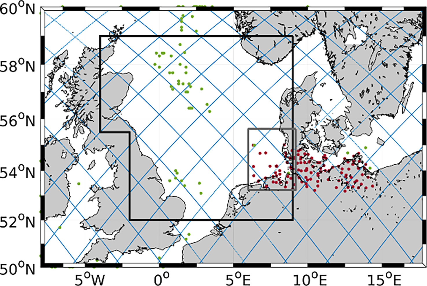
Positions of the observational data. Red dots are the DWD stations, green dots indicate the GTS stations, and the blue lines are the Jason-3 tracks. The grey box indicates the area of the German Bight and black box the area of the North Sea.
The ocean model data are compared with CMEMS in situ data TAC products of temperature and salinity (Copernicus Marine In Situ Tac Data Management Team, 2021). The original data set is quality controlled, but as an additional quality control, we apply a series of statistical and logical tests to the data set to detect and remove artifacts and/or measurement errors. These tests are based on the statistical characteristics (standard deviation, running mean, temporal gradients, etc.) of the observed data set and are completely independent of the simulation results. The remaining observations are temporally/spatially collocated with the 6-hourly simulation results.
3 Experimental design
The area covered in all the simulations is the North and Baltic Sea, as well as parts of the eastern North Atlantic Ocean (Figure 2). The chosen lateral boundary forcing for NEMO in this study is only available at the south edge of the grey box. The area coupled to CCLM but the same for NEMO and WAM in order to be more consistent and have as less disturbances as possible for CCLM. The horizontal resolution of the bathymetry is 0.06° in the longitudinal direction and 0.03° in the latitudinal direction. The CCLM area is just large enough to cover the wave model area. CCLM has a horizontal grid resolution of 0.0625° and 40 vertical grid levels. CCLM runs with a time step of 60 s, WAMs with a time step of 30 s, and NEMO with a time step of 90 s.
Figure 2
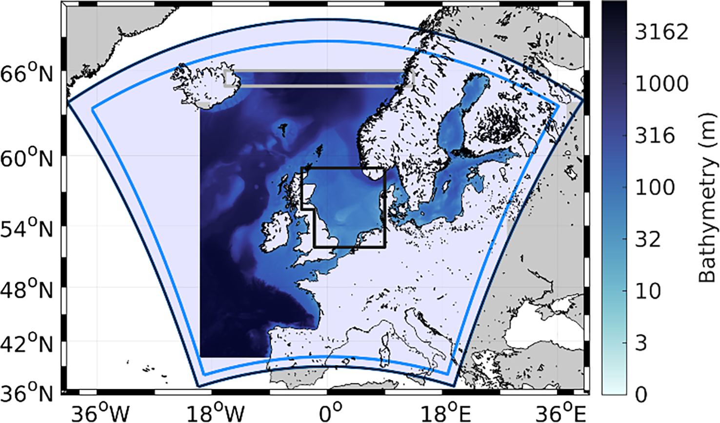
Bathymetry of the wave model WAM (shaded) and domain of the CCLM regional climate model (dark blue box). The area between the dark and light blue boxes is regarded as the buffer zone and is neglected in the analysis. The black box indicates the area of the North Sea. The grey box indicates the area, which is part of the WAM bathymetry but not the NEMO bathymetry.
As boundary and initial conditions for the atmospheric model, ECMWF Reanalysis Version 5 (ERA5) data are used (Hersbach et al., 2020). In all simulations, spectral nudging at the top of the atmosphere is used in order to keep the uncertainty due to the internal model variability low (von Storch et al., 2000; Weisse and Feser, 2003). The boundary conditions for the wave model stem from a simulation with a coarser model, which covers the whole North Atlantic ocean driven by ERA5 winds. The spectral resolution of the coarser wave model is the same as for the fine model used in this study and has a spatial horizontal resolution of 0.25°. The wave model performs a cold start in the beginning of December 2016. For the lateral boundary conditions of the ocean model, hourly CMEMS FOAM AMM7 model output (O´Dea et al., 2012) is used. For that, the NEMO ‘BDY’ standard is used. For the tracers (temperature and salinity), the boundary condition vertical profiles using the flow relaxation scheme (FRS) (Davies, 1976; Engedahl, 1995) are applied derived from the AMM7 model output and interpolated to the model grid. For water levels and currents, the boundary forcing is split into three components: a tidal harmonic signal, a barotropic signal, and a baroclinic anomaly profile. The tidal harmonic forcing is derived from the TPXOv8 model (OSU-OTIS; Egbert and Erofeeva, 2002). It is reconstructed for each model time-step from the tidal constituents M2, S2, N2, K2, K1, O1, Q1, P1, and M4. The barotropic forcing uses the Flather radiation scheme (Flather, 1994) at the first model lateral boundary bin, which is also used for the tidal harmonic forcing, and is derived from hourly CMEMS FOAM AMM7 model output consisting of the tidal averaged sea surface elevation and depth mean currents. The anomaly of the CMEMS FOAM AMM7 current profile with respect to the combined tidal and barotropic signal is used as the baroclinic forcing, which uses the FRS scheme. Furthermore, a tidal potential forcing with the same tidal constituents is applied over the whole model domain in addition to the lateral tidal forcing. The initial conditions for NEMO are taken from an uncoupled model simulations initialized in 2010.
The parameters exchanged between the three models are shown in Figure 3. CCLM and WAM exchange the u- and v-wind components at 10-m height as well as the roughness length. The 10-m u- and v-wind components are given from CCLM to WAM. In return, WAM sends the roughness length calculated from wave parameters back to CCLM. This exchange is likewise used in Wahle et al. (2017) and Wiese et al. (2019, 2020). The coupling time step between these two models is 300 s. In simulations coupling WAM and NEMO, WAM sends the Stokes–Coriolis forcing, momentum and energy fluxes, significant wave height, and wave period to NEMO and in return receives from NEMO the water level and sea ice fraction. This coupling has a time interval of 360 s. The coupling between WAM and NEMO is similar to that applied in Staneva et al. (2017, 2021). The coupling method between CCLM and NEMO has been used also by Ho-Hagemann et al. (2020). The coupling time step between these two models is 3,600 s. The parameters given from CCLM to NEMO are 10-m u- and v-wind components (only, if NEMO does not receive the momentum flux from WAM), short- and long-wave radiation, 2-m temperature, 2-m specific humidity, rain, snow, MSLP, momentum fluxes, and latent and sensible heat fluxes. NEMO then gives back the SST, sea ice parameters such as ice fraction and albedo, and the heat fluxes. Therefore, there is a mutual exchange of heat fluxes amongst the three model compartments. Within each model, the arithmetic mean of the internally calculated heat fluxes and the received heat fluxes is used. The goal of this mutual exchange is to keep the consistence of the heat fluxes, and thus the heat exchange. In order to estimate the impacts of the AOW coupling compared with the two-way-coupled model setup, three simulations are carried out, which are summarized in Table 1. In AOW, the full exchange between all models is enabled, whereas in AO, WAM does not send any information to the other two models. That way, the impact of the inclusion of the wave model into the system of atmosphere and ocean model can be examined. Furthermore, to compare the impacts of the wave and ocean model in magnitude and sign on the atmospheric model, a simulation where the ocean model is not included and the only exchange is between WAM and CCLM is performed, which is called AW. All three model simulations are initialized in the beginning of December 2016 and run until the end of December 2018.
Figure 3
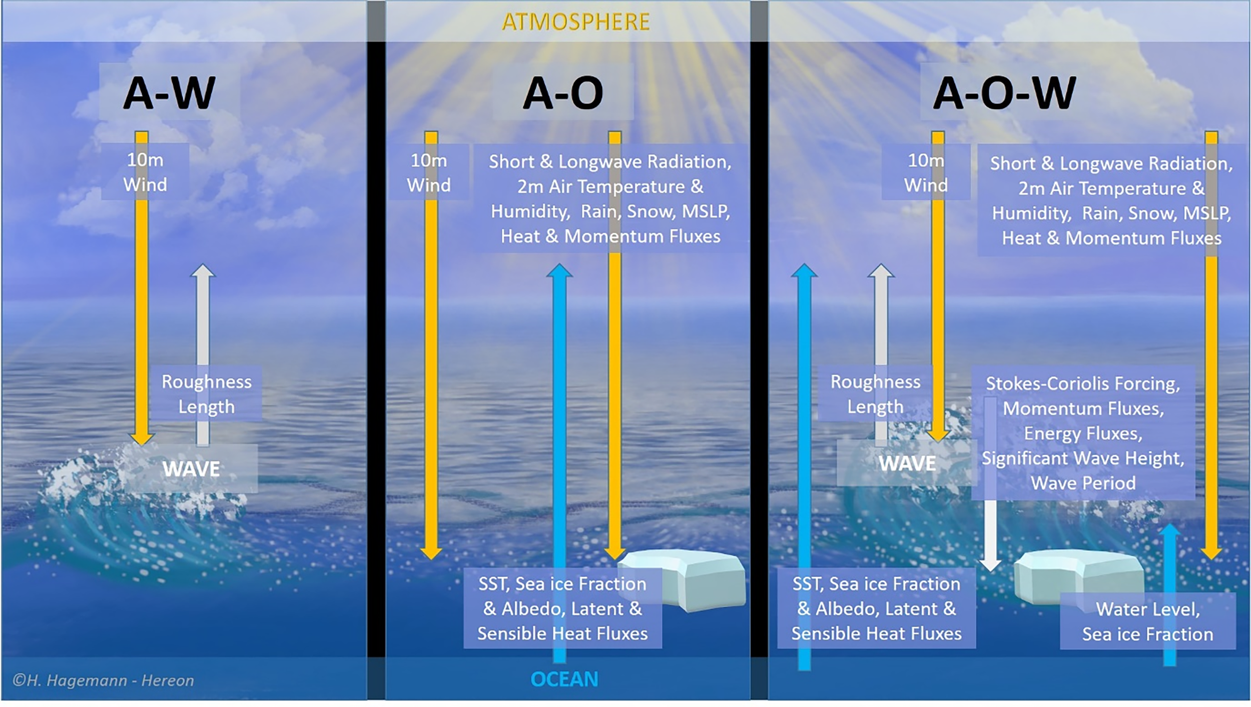
Exchanged parameters between atmosphere–wave (AW); atmosphere–ocean (AO); and atmosphere–ocean–wave (AOW).
Table 1
| Name | CCLM | WAM | NEMO | |||
|---|---|---|---|---|---|---|
| Send | Receive | Send | Receive | Send | Receive | |
| AOW | All | All | All | All | All | All |
| AO | All | NEMO | Not included | Wind/Ice | All | CCLM |
| AW | WAM | WAM | CCLM | CCLM | Not included | |
| AWT | All | All | CCLM | All | All | All |
Simulations.
4 Results
4.1 Influence on monthly mean values
Firstly, we compare monthly mean time series of MSPL, ff_10m, T_2m, roughness length (Z0), and SST averaged over the North Sea area of the three simulations (Figures 4A, C, E, G on left column) as well as the differences of AO and AW with respect to AOW. In Figures 4B, D, F, H in the right column, a rather clear seasonal cycle with two main peaks in winter and summer months can be seen, not only in the mean of the considered variables but also in the differences.
Figure 4
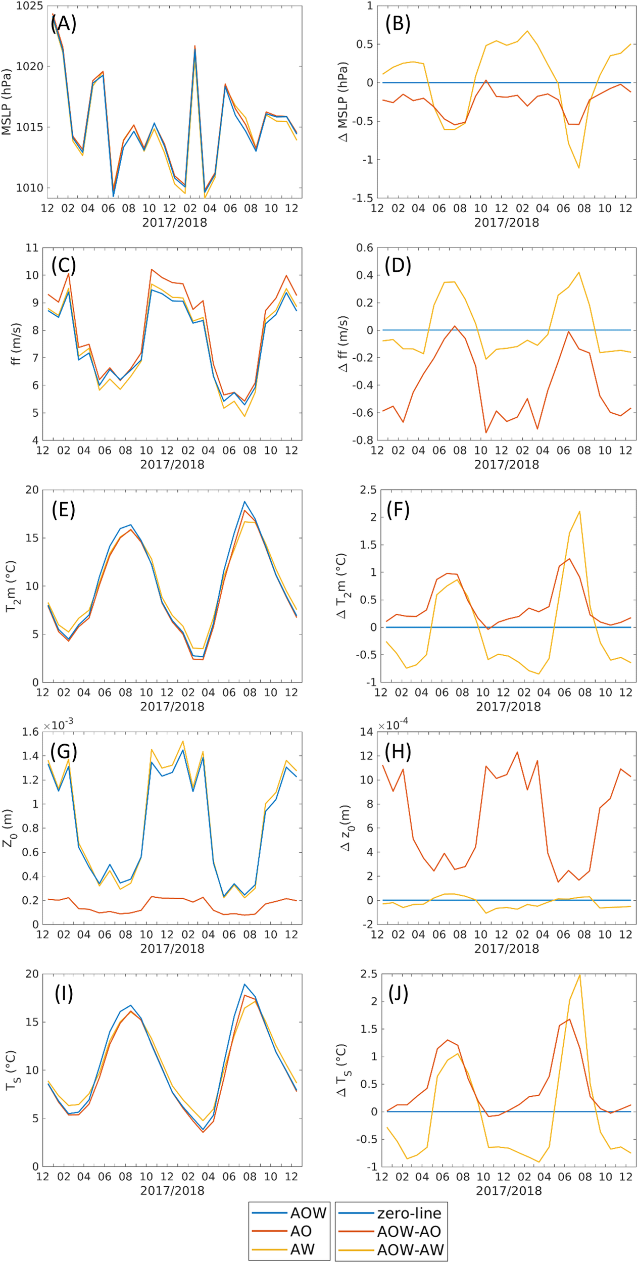
Time series of monthly mean of mean sea level pressure (A), 10-m wind speed (C), 2-m air temperature (E), roughness length (G), and surface temperature (I) within the North Sea area for all three simulations as well as the differences with respect to AOW, which is represented by the zero line (B, D, F, H, J). The time series represent equally weighted averages.
Figure 4 left column shows that in general, over the North Sea, MSLP, ff_10m, and Z0 have the high peak in winter and the low peak in summer. It is the opposite for T_2m and SST, meaning coldest in winter and warmest in summer.
Figure 4 right column displays the deviations of AOW from AO (AOW-AO, red line) and of AOW from AW (AOW-AW, orange line) to investigate the waves and the ocean coupling impacts, respectively. We analyze these impacts in the winter and summer seasons as following:
Winter
-
Waves effect: AOW-AO (red lines) shows that including waves does not affect much MSLP, T_2m, and SST but reduces ff_10m of around 0.6 m/s and increases Z0 of around 11 × 10-4 m. The enhancement of the roughness length due to the coupling with the waves is corresponding to a dominant reduction of the wind speed (Figures 4D, H).
-
Ocean effect: the waves coupling is in both AOW and AW experiments; therefore, the ff_10m and Z0 in AOW are not much different compared with those in AW (see AOW-AW, orange line). However, coupling to an ocean increases MSLP of around 0.5 hPa and reduces T_2m and SST around 1 degree (Figures 4B, F, J). During the winter months, the SST coming from NEMO (in AOW or AO) is colder than the one of ERA5 seen by CCLM if not coupled with NEMO (AW), so the coupling with the ocean cools the atmosphere.
Summer
-
Waves effect: including waves does not affect much ff_10m and Z0 (Figures 4D, H) due to a fact that the absolute values of ff_10m and Z0 are rather small in this season (Figures 4C, G). However, the waves coupling causes a reduction of MSLP (ca. 0.5 hPa), and an increase of T_2m (ca. 1°C) and SST (ca. 1.5°C). Therefore, in the AOW-coupled system, the wave models impact on the MSLP, T_2m and SST is more pronounced in the summer months than in the winter months.
-
Ocean effect: including ocean also reduces MSLP (ca. 0.5–1 hPa) and increases T_2m (ca. 1–2°C) and SST (ca. 1–2.5°C), similar to the case of including waves, although the magnitudes of modification are larger when ocean is coupled. Moreover, including ocean increases ff_10m (ca. 0.4 m/s), whereas not much modification of ff_10m is found in the case of AOW-AO. One can interpret here that the change of wind speed at the 10-m height in summer is due to the interaction between atmosphere and ocean.
During the summer months, T_2m is very similar in AO and AW, whereas AOW deviates (Figures 4E, F), which indicates that both models, the wave and the ocean, are needed to affect T_2m during summer. This is similarly seen in the SST (Figures 4I, J). The combination of all three components in AOW lets the waves affect the sea surface temperature in the ocean model, which in return also affects the 2-m air temperature. Hence, the differences in the 2-m air temperature resemble the differences in the surface temperature, which allows us to assume that the warming of the atmosphere is strongly related to the warmer SST.
This warming impact of the wave model on the SST has already been discussed in previous publications. Breivik et al. (2015) found this warming of SST in summer for the extratropical region and attributed the colder SST in the uncoupled NEMO setup to a too vigorous mixing. Zhang et al. (2011, 2012) also noted that in an uncoupled coastal ocean circulation model, considering surface wave breaking parameterization greatly enhances turbulent mixing and deepens the surface boundary layer of the temperature, and therefore, cools down the SST in the Yellow Sea in summer. Alari et al. (2016) discussed a warming in SST for the Baltic Sea and found that this is partly due to a too high wave breaking parameter in the uncoupled NEMO and partly due to taking the wave-dependent momentum flux into account in the coupled NEMO-WAM setup. Therefore, the warming of SST due to the inclusion of the waves into the coupled system in the present study is in line with earlier publications. This warming of SST then in return also affects the atmosphere lying aloft. The abovementioned studies indicated that the too vigorous mixing in the ocean model led to the colder SST in summer. This is also confirmed in the present study. For example, Figure 5 shows the difference in simulated mixed layer depth between AOW and AO NEMO for the winter (December, January, February, DJF) and summer (June, July, August; JJA) months of 2017 and 2018. In winter (Figure 5A), the estimates are similar for most parts of the North Sea, although differences of more than +/- 6 m are observed in some small areas. During the summer month (Figure 5B), it is clear that the depth of the mixed layer estimated by AO NEMO is systematically 1–3 m deeper than in the AOW run. This explains for the warmer SST in summer in AOW compared with the one in AO.
Figure 5
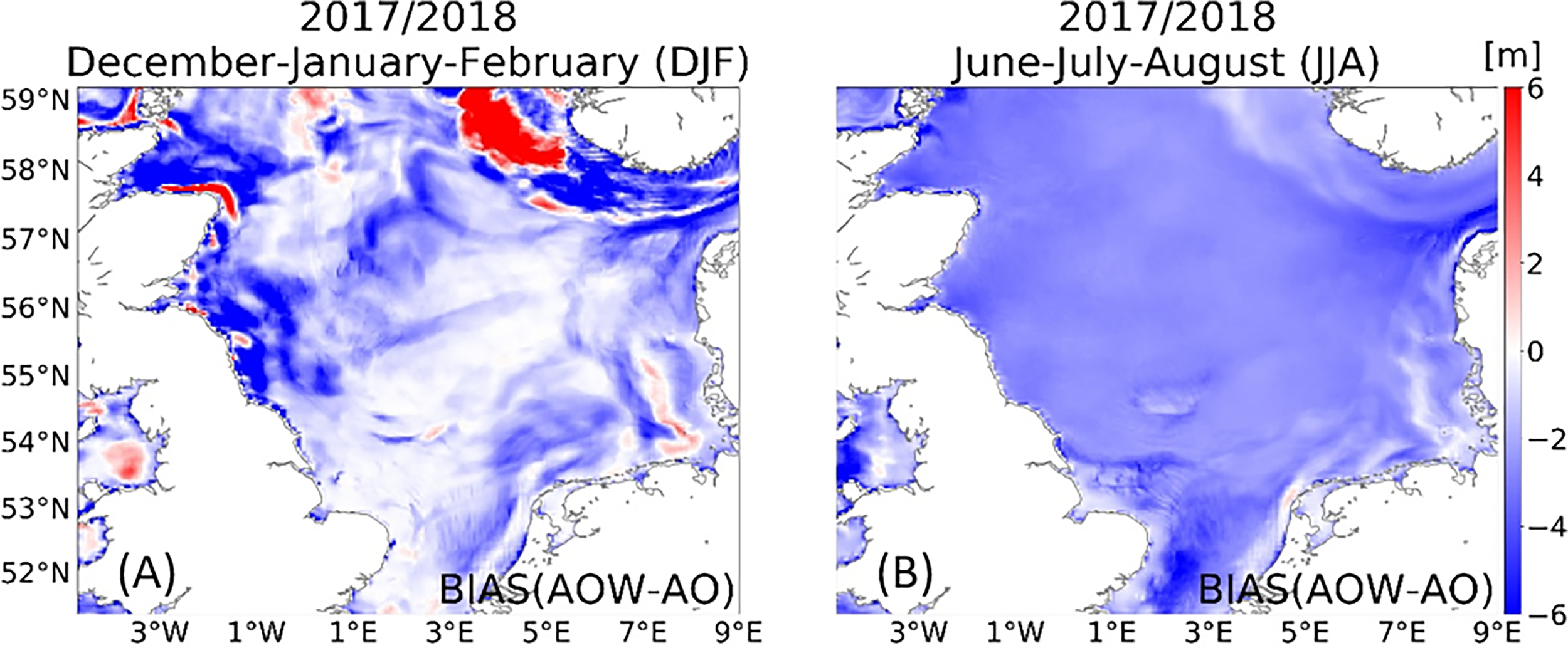
Bias of simulated mixed layer depth between AOW and AO for the winter months (A; December, January, February; DJF) and summer months (B; June, July, August; JJA) of 2017 and 2018.
To evaluate how far the impact of the waves on the system consisting of atmosphere and ocean spreads vertically, Hovmöller diagrams are shown for the monthly mean averaged over the North Sea area (Figure 6). The Hovmöller diagrams are shown for the differences between AOW and AO in order to illustrate the impacts the wave model has, when adding it to a system already consisting of atmosphere and ocean. Here, it can be seen that the impacts have the largest magnitude near the surface, but the changes due to the inclusion of the wave model can still be detected at higher levels of the atmosphere. Especially in air pressure and air temperature, the differences between AOW and AO reach quite far upward even in the monthly mean averaged over the entire North Sea area. Also during summer, where the impacts at the surface are larger than during the rest of the year, the impacts reach further upward. Furthermore, the magnitude of the impacts decreases with altitude, with a slight increase again with the opposite sign. Therefore, the inclusion of WAM impacts not only the surface layers of the atmospheric model but also the interior of the atmosphere.
Figure 6
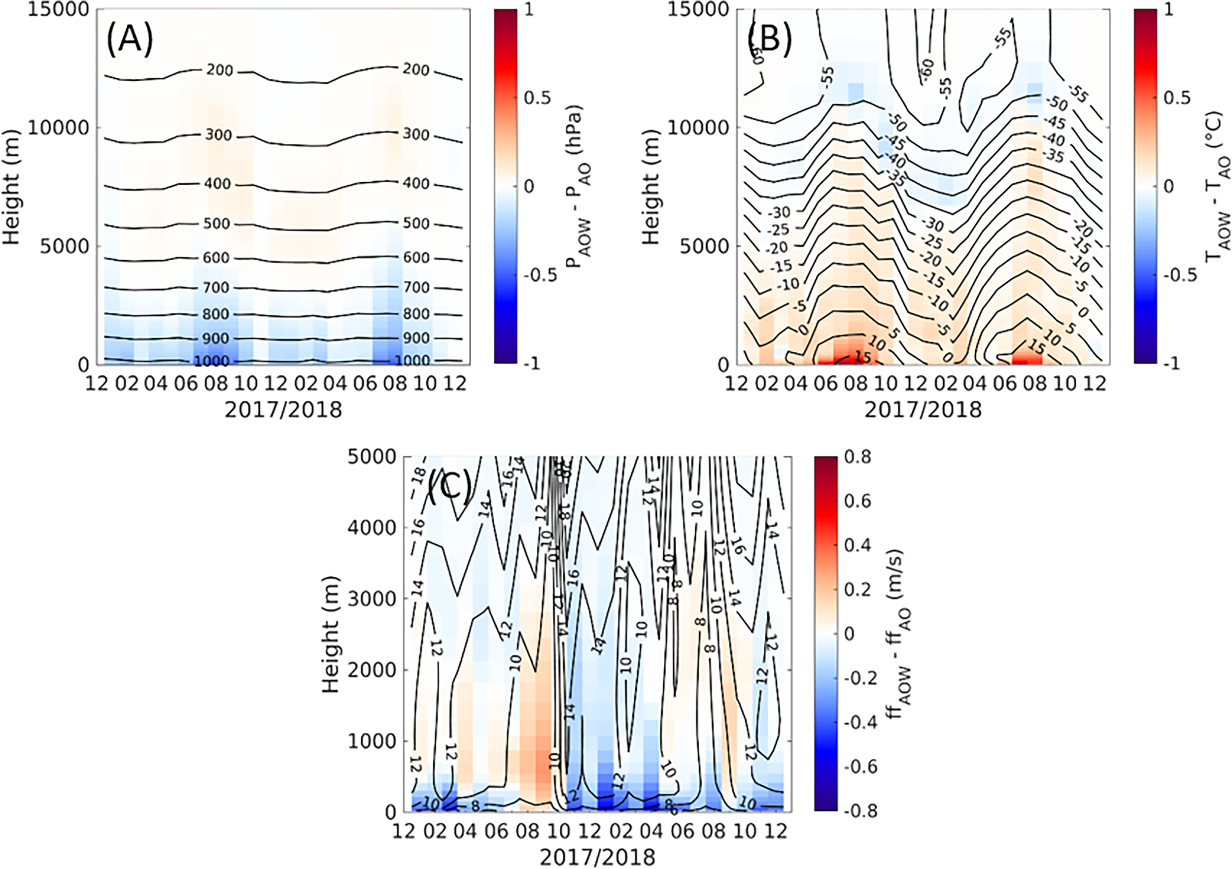
Hovmöller diagrams of air pressure (A), air temperature (B), and wind speed (C) in AOW (contour) as well as the difference between AOW and AO (shaded) within the North Sea area.
Hence, the direct impact of the waves on the roughness length and then the wind speed is largest during the winter months, where the storms and high wind speeds occur. This effect has already been discussed in publications using a coupled system of CCLM and WAM (e.g., Wahle et al., 2017; Wiese et al., 2019; Wiese et al., 2020). Hence, this study now focuses on the summer months, where the wave model influences the atmosphere by affecting the ocean. The indirect influence of waves on the atmosphere, which is composed of their direct influence on the ocean simulation and the exchange between ocean and atmosphere, is greater in the summer months and is particularly visible in the changes in air temperature. We will focus on this indirect impact of waves in the next section.
4.2 Indirect impacts of waves on the atmosphere by affecting theocean during summer
The impact the wave processes have on the AOW-coupled system on the atmosphere is studied in more detail for the summer months. During this time of the year, the changes in roughness length due to the coupling with the waves are rather limited compared with the winter. Therefore, the waves have to affect the atmosphere through other ways rather than the direct effects due to the changed roughness length. One option is to change the simulation of the ocean and thus the parameters passed from the ocean model to the atmospheric model.
In order to get a better idea of the impacts in summer, time series of differences of MSLP, 2-m air temperature, surface temperature, sensible heat flux (ASHFL), and latent heat flux (ALHFL) over the water points of the North Sea area for the summers of 2017 (Figure 7) and 2018 (Figure 8) are evaluated. During both summers, the mean impact of adding the wave model to the system is a reduction of MSLP within the North Sea area. Throughout the season, events occur, where the impact is particularly large. These events usually are during times with relatively lower MSLP. Hence, the low-pressure systems tend to get deepened, when the wave interaction is added to the system (Figures 7A, B, 8A, B). During the shown two periods, adding the ocean to a coupled system of atmosphere and waves acts into the same direction as adding the wave interaction to the system of atmosphere and ocean reducing the MSLP, but the magnitudes of the differences are larger, when adding the ocean model than when modifying the ocean model by wave–ocean interactions.
Figure 7
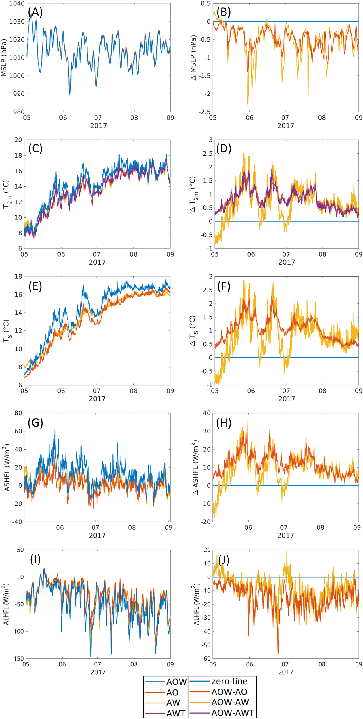
Time series of hourly values (left side) as well as differences with respect to AOW, which is represented by the zero line, (right side) of MSLP (A, B), 2-m air temperature (C, D), surface temperature (E, F), sensible heat flux (G, H), and latent heat flux (I, J) in the North Sea for summer 2017. Sensible and latent heat fluxes are positive downward. The time series represent equally weighted averages.
Figure 8
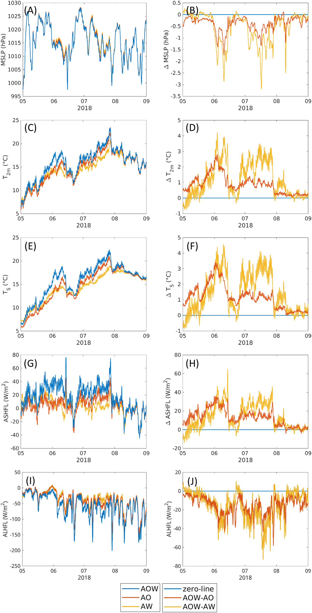
Time series of hourly values (left side) as well as differences with respect to AOW, which is represented by the zero line, (right side) of MSLP (A, B), 2-m air temperature (C, D), surface temperature (E, F), sensible heat flux (G, H), and latent heat flux (I, J) in the North Sea for summer 2018. Sensible and latent heat fluxes are positive downward. The time series represent equally weighted averages.
During the summer months, the overall impact of adding the waves to the coupled system is a warming of the air over the North Sea (Figures 7C, D, 8C, D). The strength of this warming varies with time and has some peaks, where it is particularly strong. The warming in air temperature is resembled in the surface temperature (Figures 7E, F, 8E, F). Here, one can guess that when including the wave model, the ocean is warmer and then warms up the atmosphere above. However, Figures 7G and 8G show positive values of ASHFL most of the time in the two summers. In the CCLM model, sensible and latent heat fluxes are defined positive downward. Thus, the positive ASHFL values mean the atmosphere transfers sensible heat to the ocean. In both cases of AOW-AO and AOW-AW, the positive differences of ASHFL are often seen (Figures 7H, 8H). This explains why SST of AOW is warmer than AO and AW in these summer days. The August of 2018 has negative ASHFL, but during this month, the three experiments (AOW, AO, AW) have a very small difference in ASHFL.
If the sensible heat flux in summer is not from ocean to the atmosphere, how is the atmosphere warmed up, not only near the sea surface but also upward to high levels interior of the atmosphere (Figure 6B)? Our speculation is that near the sea surface, due to the warmer SST in AOW than in AO and AW, the longwave upward radiation from the sea surface to the atmosphere in AOW is higher, and due to that fact, the near surface air temperature is warmed up in AOW more than in the other two experiments. At higher levels in the atmosphere, the increase of air temperature could partly be explained by the upward propagation of the near surface warm air or partly be attributed to the increase of the latent heat flux from the ocean to the atmosphere. Figures 7I and 8I show large latent heat fluxes in summer in all three experiments. AOW has the larger ALHFL than AO and AW, except in some few days (Figures 7J, 8J). This means that when the wave model is coupled to both atmospheric and ocean models, the SST is warmer, causing more evaporation from the sea surface; therefore, larger latent heat flux is transferred from ocean to the atmosphere. This certainly leads to a somewhat cooling down of SST. However, the latent heat flux sent to the atmosphere also means that the humidity of the atmosphere increases due to the evaporation. The vapor will condense somewhere inside the atmosphere and release energy to the atmosphere. This moistening, and then warming, makes the air buoyant, driving low-level baroclinicity and atmospheric convection, deepening the MSLP (Figures 7B, 8B). This process may explain for the warming upward into the high levels of atmosphere (Figure 6B). In addition, when the atmosphere is warmed up, which is much faster than the warming up of the sea surface, the temperature vertical gradient between the atmosphere and the ocean also increases, leading to the positive ASHFL, and therefore, a warmer SST.
To underline the assumption that the warming is due to the coupling between the wave and ocean model, an experiment where the feedback from WAM to NEMO is disabled has been carried out for the summer of 2017 (AWT). The results of that experiment are very close to the results of AO. This implies that the warming indeed is due to the coupling of the wave to the ocean model, which then feedbacks to the atmosphere. Hence, the warming of the ocean surface due to the inclusion of the wave interaction into the system has an influence on the air temperature and by that further processes within the atmosphere, also changing the MSLP. Another point standing out, when analyzing the time series of MSLP, temperatures and sensible heat flux, is that the two two-way coupled simulations AW and AO yield quite similar results during summer, whereas the coupled simulations including all three components stands out from the other two, which again indicates that both models are essential for impacting the air temperature in this case (Figures 7C, D).
Some of the peaks in changes in air temperature correspond to peaks in decreased MSLP (May 2017). Other peaks in air temperature rise are a couple of days prior to the drop in MSLP (June 2018). This is investigated in more detail in the next section.
4.3 Case studies
4.3.1 Event with the origin of changes outside the North Sea area
In the end of May 2017, an event with large differences in MSLP, temperature, and wind speed within the North Sea occurred (Figure 9). For this event, the large differences in MSLP and temperature are around the same time. At that time, the center of the low was positioned in the Iceland area with a warm front (occluded front) across the North Sea. This front varies in the exact position between the model simulations and can be detected best in the 850-hPa temperature (Figure 9D). Also, where the front is embedded into the low-pressure system varies between the experiments and, hence, the structure of the low is changed (Figure 9A). Due to the differing structure of the lows in the two experiments, the wind speed especially along the front is changed as well (Figure 9E).
Figure 9
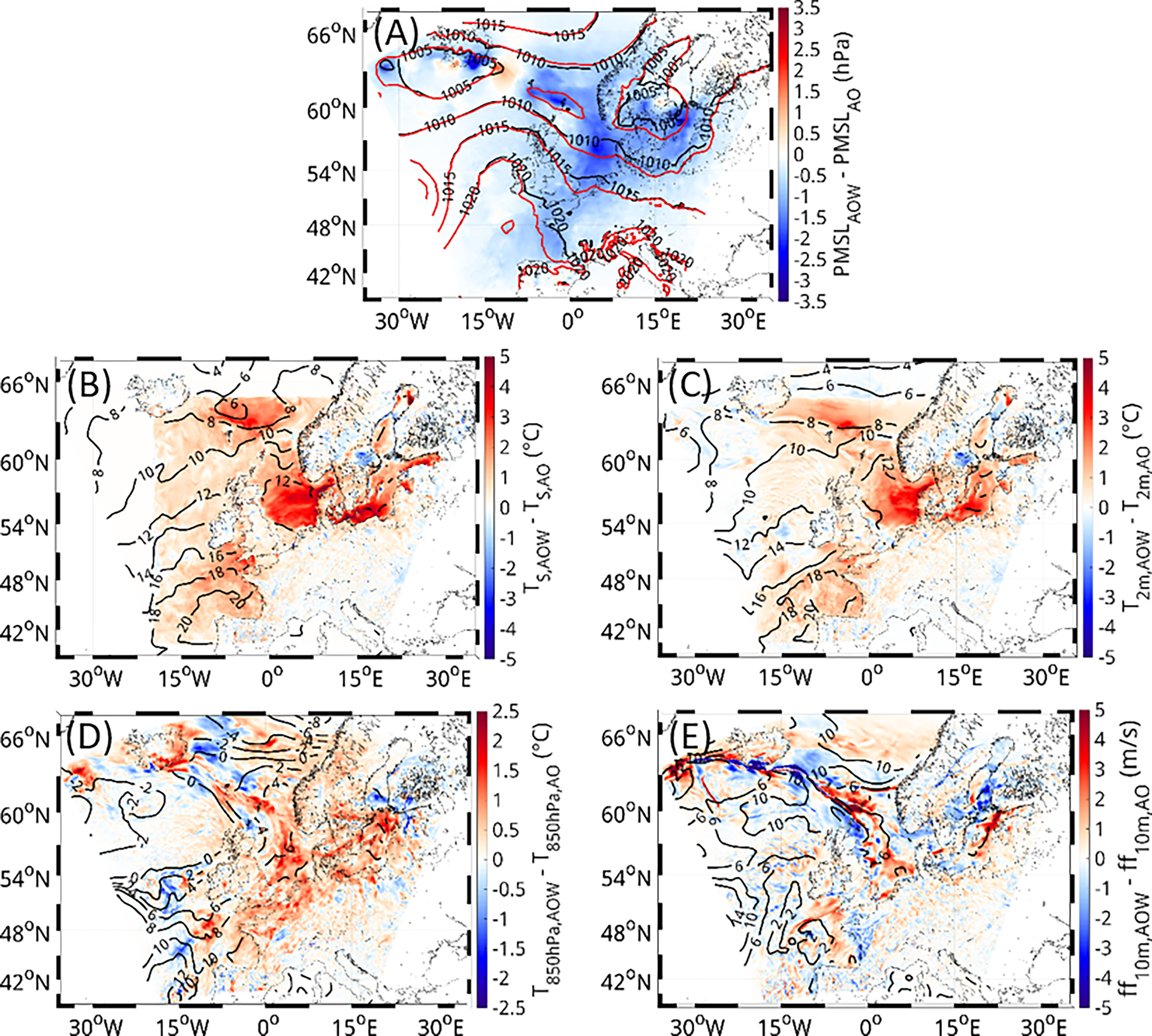
MSLP (A), surface temperature (B), 2-m air temperature (C), 850-hPa air temperature (D) and wind speed (E) on 30.05.2017 18UTC in AOW (contour plot) and the differences (shaded) between AOW and AO. The AOW data shown in the contour plots were smoothed with a window of 100 km.
These differences have their origin in the Bay of Biscay, located on the west coast of France and the north coast of Spain, a couple of days earlier (Figure 10) and can be related to the change in vertical temperature profile, as presented in Figure 6B. Due to the inclusion of WAM, the surface temperature is increased. This leads to an increase in air temperature near the surface, which penetrates also to the 850-hPa height and even higher to around 300 hPa, the position of the jet stream. The warming induces the air to rise and, hence, the MSLP to decrease. With the front approaching, this perturbation is spread along the front and transported further east to the North Sea area. The event with large changes in all three variables in the middle of May (14.05.2017) developed in a similar way.
Figure 10
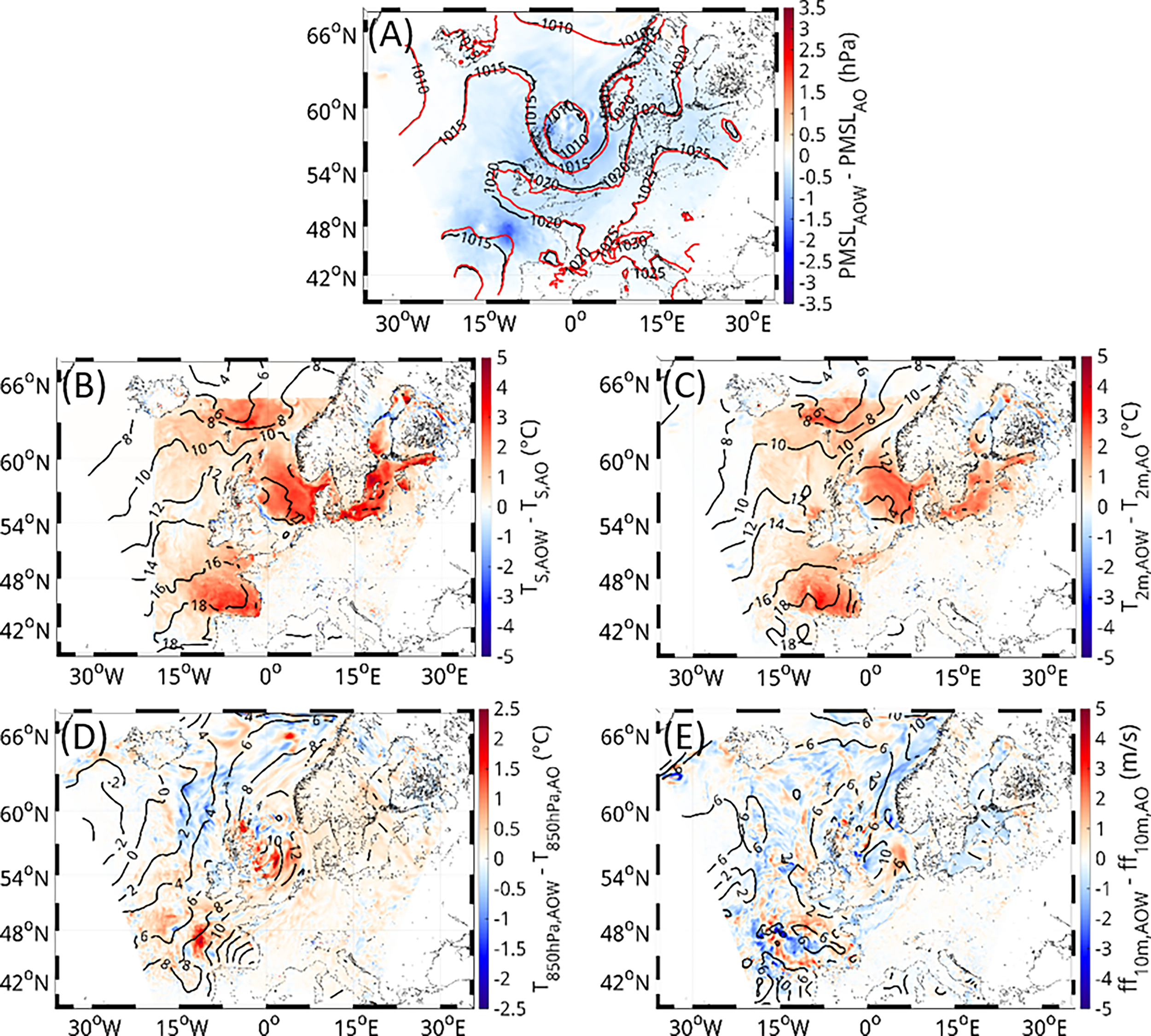
MSLP (A), surface temperature (B), 2-m air temperature (C), 850-hPa air temperature (D) and wind speed (E) on 28.05.2017 00UTC in AOW (contour plot) and the differences (shaded) between AOW and AO. The AOW data shown in the contour plots were smoothed with a window of 100 km.
4.3.2 Event with the origin of changes within the North Sea area
On June 10, 2018, an event with low pressure in AOW and AO within the North Sea area occurred (Figure 11). At that time, a very shallow low pressure system was situated over the North Sea, which is deeper in AOW than AO (Figure 11A). Unlike the changes in May 2017, which originated in the Bay of Biscay, the changes during this event originate within the North Sea. This might also be the reason why the peak in temperature change is prior to the peak in MSLP changes. The SST is warmer in AOW than in AO (Figure 11B) due to the inclusion of the wave interactions into the system. The warming in SST leads to a warming in the 2-m air temperature (Figure 11C). The warming of the air near the surface enhances the rising of the air in the center of the low, which results in the deepening of the low.
Figure 11
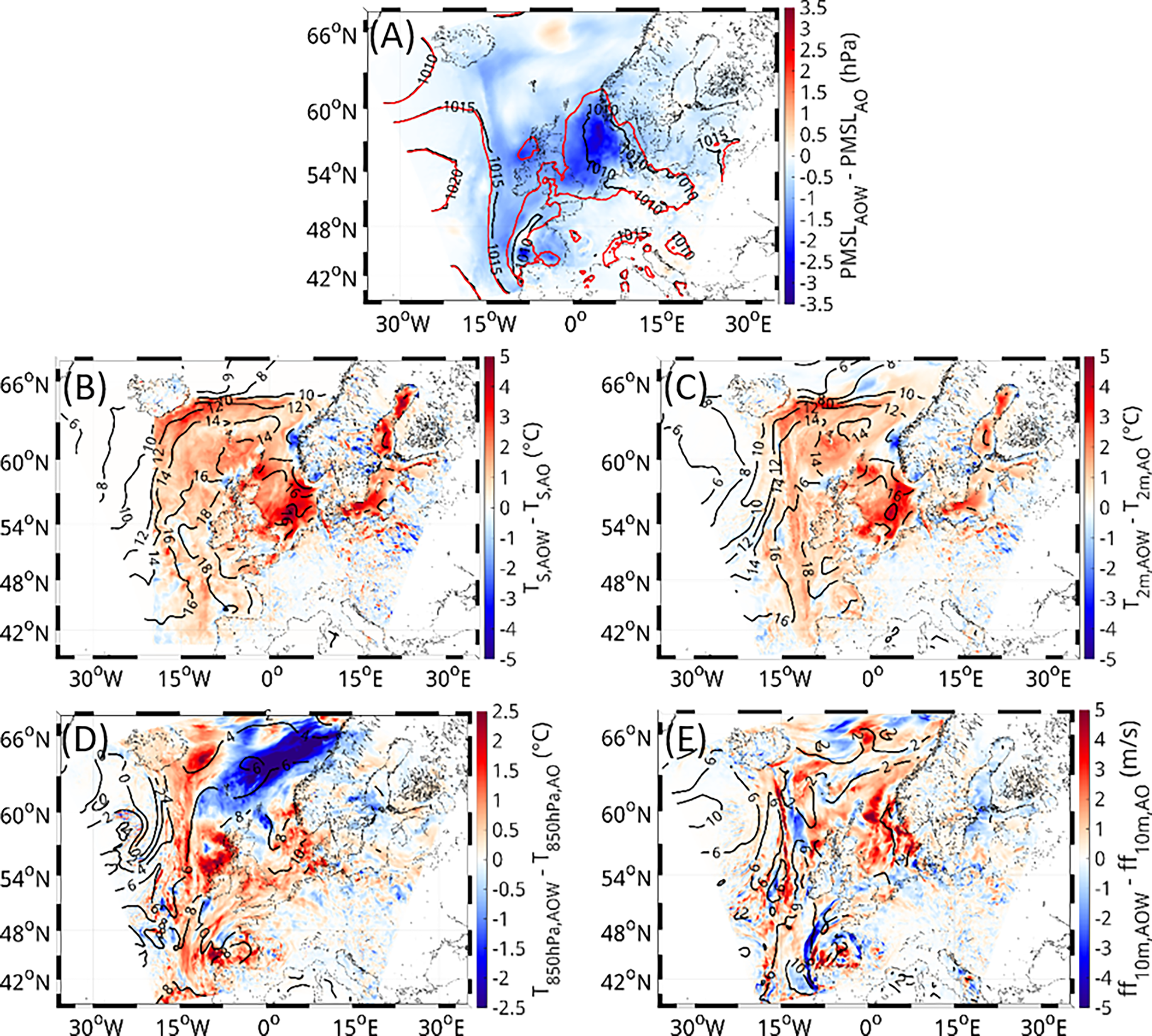
MSLP (A), surface temperature (B), 2-m air temperature (C), 850-hPa air temperature (D) and wind speed (E) on 10.06.2018 06UTC in AOW (contour plot) and the differences (shaded) between AOW and AO. The AOW data shown in the contour plots were smoothed with a window of 100 km.
4.4 Comparison with observations
In order to evaluate how these changes due to the full coupling impact the realism of the simulations, the model results are compared with observations. The general agreement of the model simulations with the data is good, with only small variations between the three simulations. (Scatter plots comparing DWD observational data with simulated 10m wind speed, 2m air temperature, and MSLP are included in the Supplementary Material. When comparing the time series of stations within the German Bight area for the month of May 2017, differences between the simulation results become more visible. Especially, for the event at the end of May, AOW has the best agreement with the observations concerning the MSLP. The temperature and wind speed, however, are over- and underestimated, respectively (Figure 12). However, the differences between the simulations in general are quite small and only become visible for events, where AOW really differs from the other simulations. In all three parameters, events occur where AOW performs better than the other configurations, but also events where the other configurations perform better than AOW.
Figure 12
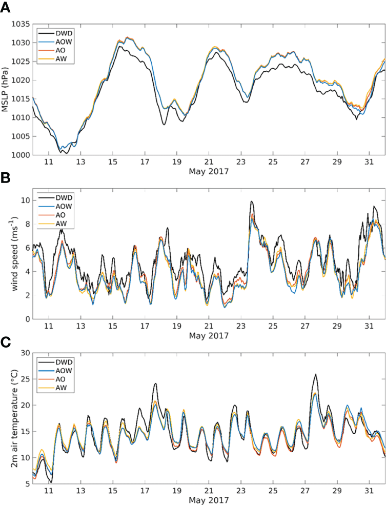
Time series of the MSLP (A), 10-m wind speed (B), and 2-m air temperature (C) averaged over the DWD stations in the German Bight.
The largest changes in the overall performance of the model system become visible in the wind speed and, hence, in the significant wave height (Figures 13A, C, E). When comparing the simulated wind speed to GTS and Jason-3 measurements within the North Sea area, the two simulations including the wave–atmosphere exchange perform better than AO. AO overestimates the wind speed, especially the high wind speeds, which is gone in AOW and AW. AOW and AW, however, slightly underestimate the extreme events (Figures 13A, C). Still, AOW and AW have better bias, SI and RMSE than AO. This is straight resembled in the significant wave height in WAM (Figures 13B, D, F). Both simulations where the wave model sends data to the atmospheric model perform better than AO, especially the overestimation of the extremes, is gone.
Figure 13
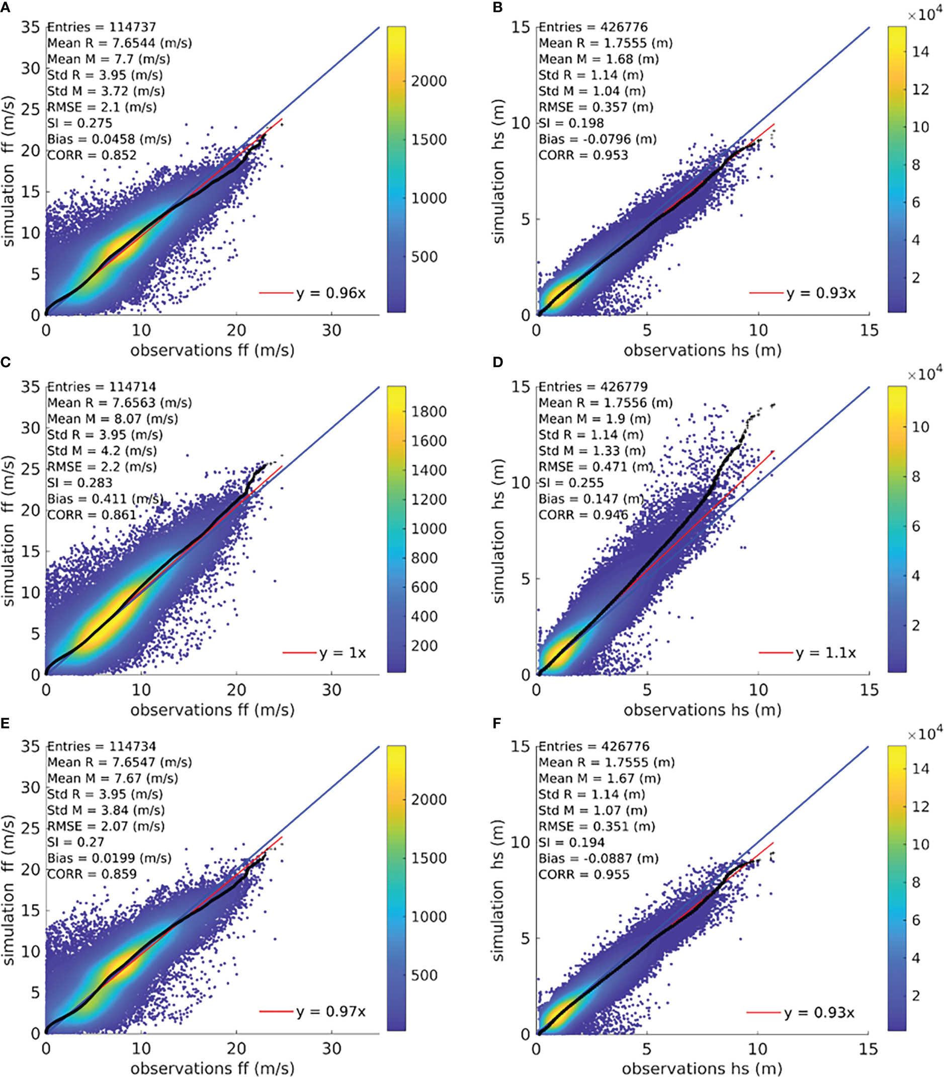
Q–Q scatter plots for the measured (GTS, J3) (reference, R) and modelled (M) wind speeds (left side) and significant wave height (right side) in the North Sea for AOW (A, B), AO (C, D), and AW (E, F). The Q–Q plot is shown as black crosses, the 45° reference line is indicated by the blue line, and the least squares line with the best fit is the red line.
When comparing AOW and AO with ocean observations for temperature and salinity, the model agreement with the observations is really good in both cases, here shown exemplary for the NsbII station (Figure 14). The images show the simulated data as Hovmöller diagrams in the shaded background and the collocated observations as colored dots in the foreground. The color coding is the same for both data sets. The warmer temperatures of AOW (Figure 14A) in summer, when the North Sea starts to heat up, can be seen in those comparisons as well. This warmer temperature generally results in a better agreement with the observations. Especially, the events in the beginning of June 2018, where the ocean temperature is warmer in AOW than AO, are present in the observations as well, with AOW having the better agreement. However, at times, especially during the cooling phase in autumn and early winter, AO can also have a better agreement with the observations. There are some rapid temporal changes of 1°C to 2°C in the cold or cooling period (February–March 2017, September–October 2017, and November–December 2018) of the temperature observations shown that are not reproduced in any of the simulations. It is uncertain whether these signals are erroneous or reliable measurements. In our opinion, we cannot be 100% certain that these changes are not caused by lateral warm/cold water intrusion, and they have been retained in the images for consistency. For the salinity, both simulations perform similarly (Figures 14C, D). At times AOW is closer to the observations and at other times AO. During those 2 years, AOW is closer to the observations during winter, whereas AO performs better in spring.
Figure 14
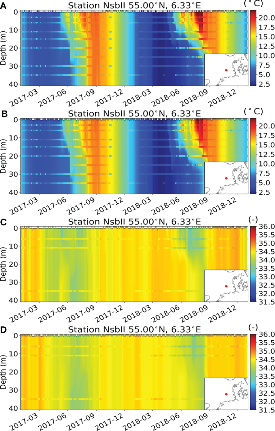
Comparison between model and observational data at NsbII for AOW and AO for ocean temperature (A, B) and salinity (C, D), respectively. The images show the simulated data as Hovmöller diagrams in the shaded background and the collocated observations as colored dots in the foreground. The color coding is the same for both data sets.
5 Discussion and conclusions
In this study, the effects of full coupling of atmosphere, waves, and ocean compared with two-way-coupled simulations of either atmosphere and wave or atmosphere and ocean models are analyzed. The effects of including the waves into the system consisting of atmosphere and ocean model, or including the ocean into the system consisting of atmosphere and wave model on the MSLP, ff_10m, and T_2m, vary throughout the year. The largest effect on the wind speed has the inclusion of the wave model into the system during the winter months. When the wind speeds are high, the wind speed reduction due to the roughness length being estimated from wave parameters instead of wind is the largest. This has also been found in previous studies using coupled wave–atmosphere models (Wahle et al., 2017; Wu et al., 2017; Wiese et al., 2019; Varlas et al., 2020; Wiese et al., 2020) and in a study by Gentile et al. (2021) using an AOW-coupled model, where they concluded that under high wind conditions, the wave models’ impact on the 10-m wind speed is much larger than the ocean models’ impact. During the summer months, however, the effect of the waves on the wind speed becomes quite small. During that time, the ocean has a larger effect with an enhancement of the wind speed within the North Sea area. Hence, whereas the wave models effect on wind speed is large during the storm season, the ocean models’ impact is larger during summer, the wave and the ocean model take turns in having the dominant effect on the atmosphere.
The effect on T_S and, hence, on T_2m in summer is a warming regardless of adding the waves or the ocean into the system. This warming is due to the interaction of the waves and the ocean, enhancing the SST in AOW, whereas AO and AW have similar surface temperatures. The warming of the SST due to the interaction of wave and ocean models has already been found in previous studies using coupled wave and ocean models (Breivik et al., 2015; Alari et al., 2016). During winter, however, the waves’ impact on the temperature is fairly small, whereas NEMO has a colder SST than the SST from the forcing data and, hence, cools the atmosphere.
For the MSLP, again both models are needed to reduce the MSLP over the North Sea during the summer months, which is in line with the warming during that time. During the winter, however, the two models have opposing effects on the atmosphere. While the cooling of the ocean model leads to a slight increase in MSLP, the inclusion of the wave model leads to a slight reduction of the MSLP.
The effects of the wave and the ocean model on the atmosphere vary throughout the year in a similar way in both years simulated in this study. Furthermore, which model has the dominant effect on the atmosphere varies by season and variable considered. In conclusion, to affect the T_2m air temperature during the summer months, in this case, the full coupling between all three models is needed, since the interaction between the wave and ocean model is essential to affecting the SST and in consequence also the air temperature. These impacts also spread into higher parts of the atmosphere.
Note that the described effects of including a wave model in the coupled system consisting of an atmosphere and an ocean model can only be understood by considering the parameterizations of the models, the coupling approach, and the experimental setup. Wu et al. (2019) conducted a study with AOW-coupled experiments for the North Sea area. While they concentrated on the effects of the coupling during 2-month-long simulations of January and July 2015, we conducted 2-year-long simulations, showing that the impacts of the coupling are similar during both years. Wu et al. (2019), however, found in their study some opposing results to ours, with a cooling of the SST in summer and a warming of the SST during the winter months due to the coupling between the wave and ocean model. This opposing result is the case, since in their model setup, consisting of the Weather Research and Forecasting (WRF) Model as an atmospheric model, WaveWatch-III as the wave model, and NEMO as the ocean model, the upper ocean mixing is enhanced, when the wave model is coupled to the ocean model. Furthermore, Gronholz et al. (2017) used the coupled ocean–atmosphere wave sediment transport system (COAWST) consisting of the atmospheric model WRF, the Simulating Waves Nearshore (SWAN), and the Regional Ocean Modeling System (ROMS) for the simulation of a storm event in the North Sea. Their results also indicated that including estimates from the wave model increases vertical mixing in the ocean model. However, due to the complexity of comparing different experimental designs, the authors would not in this study. Another example is that in the present study we only couple the roughness length from the wave model to the atmospheric model. Zou et al. (2019) showed that the wave coherent stress exerted by surface waves can account a larger portion of total wind stress, whereas the roughness length of wave-based parameterization only depicts the turbulent stress. We will consider sending the momentum/stress from either the wave or ocean model to the atmospheric model and investigate their effects on the coupling in our next study.
Our present study shows that for simulating some processes, the whole system consisting of atmosphere, waves, and ocean has to be used in order to account for the proper feedback. Here, especially the ocean temperature is affected by the waves, which in turn also affects the overlying atmosphere. In a next step, it has to be analyzed in more detail what the effects on the ocean and on the waves are. Also, as in the study of Gentile et al. (2022) on a convective scale, ensembles can be used to estimate the uncertainty of the fully coupled system on the mesoscale, as it has already been shown that the coupling between CCLM and NEMO as well as CCLM and WAM reduce the internal model variability of CCLM (Ho-Hagemann et al., 2020; Wiese et al., 2020). The inclusion of the wave model into the system consisting of the atmospheric model and the ocean model especially reduces errors in the wind speed representation of the atmospheric model over the North Sea and, hence, also in the significant wave height of the wave model. This can be important for forecasts for the offshore energy sector as well as shipping. Also, the more precise representation of processes at the interface of the ocean and atmosphere through the waves could become a crucial part for impact studies in future scenario simulations.
Statements
Data availability statement
The raw data supporting the conclusions of this article will be made available by the authors, without undue reservation.
Author contributions
Conceptualization: JS, SG, and AW; Data curation: SG and AW; Model development: SG and HTMH-H; Coupling development: SG and HTMH-H; Formal analysis: AW; Methodology: JS and SG; Project Supervision: JS; Validation and Visualization: AW and SG; Writing: All. All authors contributed to the article and approved the submitted version.
Funding
Project under the German Marine Research (DAM) research contract “CoastalFutures - Future scenarios to promote sustainable use of marine areas”, funded by the German Federal Ministry of Education and Research (BMBF) under grant number 03F0911A. JS acknowledges the EU H2020 and was supported by funding from the European Green Deal project “Large scale RESToration of COASTal ecosystems through rivers to sea connectivity” (REST-COAST). SG received funding from the German Marine Research Alliance (DAM) project “CoastalFutures - Future scenarios to promote sustainable use of marine areas” and from the H2020 project IMMERSE. AW was funded by the project “CoastalFutures - Future scenarios to promote the sustainable use of marine areas” of the German Marine Research Alliance (DAM). HTMH-H was supported by funding from the German REKLIM project.
Acknowledgments
The authors would like to thank Wolfgang Koch for his assistance with implementing the coupling between CCLM, WAM, and NEMO. Thanks are given to Arno Behrens for providing the boundary forcing for WAM. Furthermore, we thank Jean Bidlot from ECMWF for making the GTS data available as well as Marcel Riecker for providing Jason-3 altimeter data. The altimeter products were produced and distributed by Aviso+ (https://www.aviso.altimetry.fr/), as part of the SSALTO ground processing segment. We would also like to thank the DWD for making the observational data available through the Climate Data Centre (https://www.dwd.de/DE/klimaumwelt/cdc/cdc_node.html), as well as Copernicus for making the Ocean observations available. Thanks are also given to ECMWF and Copernicus for making ERA5 and AMM7 data available, respectively. AW and SG acknowledge Cluster of Excellence EXC 2037 “Climate, Climatic Change, and Society” (CLICCS) (project no. 390683824). The production of the results presented in this study used computational resources of the MISTRAL cluster system of the Deutsches Klimarechenzentrum (DKRZ) granted by its Scientific Steering Committee (WLA) under project ID bu1213. The responsibility for the content of this publication lies with the author.
Conflict of interest
The authors declare that the research was conducted in the absence of any commercial or financial relationships that could be construed as a potential conflict of interest.
Publisher’s note
All claims expressed in this article are solely those of the authors and do not necessarily represent those of their affiliated organizations, or those of the publisher, the editors and the reviewers. Any product that may be evaluated in this article, or claim that may be made by its manufacturer, is not guaranteed or endorsed by the publisher.
Supplementary material
The Supplementary Material for this article can be found online at: https://www.frontiersin.org/articles/10.3389/fmars.2023.1104027/full#supplementary-material
References
1
Alari V. Staneva J. Breivik Ø. Bidlot J. R. Mogensen K. Janssen P. (2016). Surface wave effects on water temperature in the Baltic Sea: Simulations with the coupled NEMO-WAM model. Ocean Dynamics66 (8), 917–930. doi: 10.1007/s10236-016-0963-x
2
Bidlot J. R. Holmes D. J. Wittmann P. A. Lalbeharry R. Chen H. S. (2002). Intercomparison of the performance of operational ocean wave forecasting systems with buoy data. Weather Forecasting17 (2), 287–310. doi: 10.1175/1520-0434(2002)017<0287:IOTPOO>2.0.CO;2
3
Bidlot J. Holt M. (2006). Verification of operational global and regional wave forecasting systems against measurements from moored buoys (Geneva: WMO & IOC).
4
Bignalet-Cazalet F. Picot N. Desai S. Scharroo R. Egido A. (2021) Jason-3 products handbook. Available at: https://www.aviso.altimetry.fr/fileadmin/documents/data/tools/hdbk_j3.pdf (Accessed 29.06.2022).
5
Bonaduce A. Staneva J. Grayek S. Bidlot J. R. Breivik Ø. (2020). Sea-State contributions to sea-level variability in the European seas. Ocean Dynamics70, 1547–1569. doi: 10.1007/s10236-020-01404-1
6
Breivik Ø. Mogensen K. Bidlot J. R. Balmaseda M. A. Janssen P. A. E. M. (2015). Surface wave effects in the NEMO ocean model: Forced and coupled experiments. J. Geophys. Res. Oceans120, 2973–2992. doi: 10.1002/2014JC010565
7
Carniel S. Benetazzo A. Bonaldo D. Falcieri F. M. Miglietta M. M. Ricchi A. et al . (2016). Scratching beneath the surface while coupling atmosphere, ocean and waves: Analysis of a dense water formation event. Ocean Model.101, 101–112. doi: 10.1016/j.ocemod.2016.03.007
8
Cavaleri L. Fox-Kemper B. Hemer M. (2012). Wind waves in the coupled climate system. Bull. Am. Meteorol. Soc.93, 1651–1661. doi: 10.1175/Bams-d-11-00170.1
9
Chen S. S. Price J. F. Zhao W. Donelan M. A. Walsh E. J. (2007). The CBLAST-hurricane program and the next-generation fully coupled atmosphere–wave–ocean models for hurricane research and prediction. Bull. Am. Meteorol. Soc.88 (3), 311–317. doi: 10.1175/BAMS-88-3-311
10
Copernicus Marine In Situ Tac Data Management Team (2021). Product user manual for multiparameter Copernicus In situ TAC (PUM). doi: 10.13155/43494
11
Davies H. (1976). A lateral boundary formulation for multi-level prediction models. Q. J. R. Meteorological Soc.102 (432), 405–418.
12
Doms G. Baldauf M. (2013). A description of the nonhydrostatic regional COSMO model. part I: Dynamics and numerics (Offenbach: Deutscher Wetterdienst).
13
DWD Climate Data Center (CDC) (2022a) Hourly station observations of wind velocity ca. 10 m above ground in m/s for Germany (Accessed 19.04.2022).
14
DWD Climate Data Center (CDC) (2022b) Hourly station observations of air temperature at 2 m above ground in °C for Germany (Accessed 19.04.2022).
15
DWD Climate Data Center (CDC) (2022c) Hourly station observations of air pressure at mean sea level in hPa for Germany (Accessed 19.04.2022).
16
ECMWF (2019). “IFS documentation CY46R1 - Part VII: ECMWF wave model.” in IFS documentation CY46R1, vol. 7 (Reading: ECMWF). doi: 10.21957/21g1hoiuo
17
Egbert G. D. Erofeeva S. Y. (2002). Efficient inverse modeling of barotropic ocean tides. J. Atmospheric Oceanic Technol.19 (2), 183–204.
18
Engedahl H. (1995). Use of the flow relaxation scheme in a three-dimensional baroclinic ocean model with realistic topography. Tellus A47 (3), 365–382.
19
Flather R. A. (1994). A storm surge prediction model for the northern bay of Bengal with application to the cyclone disaster in April 1991. J. Phys. Oceanogr.24 (1), 172–190.
20
Gentile E. S. Gray S. L. Barlow J. F. Lewis H. W. Edwards J. M. (2021). The impact of atmosphere–ocean–wave coupling on the near-surface wind speed in forecasts of extratropical cyclones. Boundary Layer Meteorol.180 (1), 105–129. doi: 10.1007/s10546-021-00614-4
21
Gentile E. S. Gray S. L. Lewis H. W. (2022). The sensitivity of probabilistic convective-scale forecasts of an extratropical cyclone to atmosphere–ocean–wave coupling. Q. J. R. Meteorol. Soc.148 (743), 685–710. doi: 10.1002/qj.4225
22
Gröger M. Dieterich C. Haapala J. Ho-Hagemann H. T. M. Hagemann S. Jakacki J. et al . (2021). Coupled regional earth system modeling in the Baltic Sea region. Earth Syst. Dynam.12, 939–973. doi: 10.5194/esd-12-939-2021
23
Gronholz A. Gräwe U. Paul A. Schulz M. (2017). Investigating the effects of a summer storm on the north Sea stratification using a regional coupled ocean-atmosphere model. Ocean Dynamics67, 211–235. doi: 10.1007/s10236-016-1023-2
24
Hersbach H. Bell B. Berrisford P. Hirahara S. Horányi A. Muñoz-Sabater J. et al . (2020). The ERA5 global reanalysis. Q. J. R. Meteorol. Soc.146 (730), 1999–2049. doi: 10.1002/qj.3803
25
Ho-Hagemann H. T. M. Gröger M. Rockel B. Zahn M. Geyer B. Meier H. E. M. (2017). Effects of air-sea coupling over the north Sea and the Baltic Sea on simulated summer precipitation over central Europe. Clim. Dyn.49, 3851–3876. doi: 10.1007/s00382-017-3546-8
26
Ho-Hagemann H. T. M. Hagemann S. Grayek S. Petrik R. Rockel B. Staneva J. et al . (2020). Internal model variability of the regional coupled system model GCOAST-AHOI. Atmosphere11 (3), 227. doi: 10.3390/atmos11030227
27
Ho-Hagemann H. T. M. Hagemann S. Rockel B. (2015). On the role of soil moisture in the generation of heavy rainfall during the oder flood event in July 1997. Tellus A67, 28661. doi: 10.3402/tellusa.v67.28661
28
Kelemen F. D. Primo C. Feldmann H. Ahrens B. (2019). Added value of atmosphere-ocean coupling in a century-long regional climate simulation. Atmosphere10 (9), 537. doi: 10.3390/atmos10090537
29
Li D. Staneva J. Bidlot J. R. Grayek S. Zhu Y. Yin B. (2021). Improving regional model skills during typhoon events: A case study for super typhoon lingling over the northwest pacific ocean. Front. Mar. Sci.8. doi: 10.3389/fmars.2021.613913
30
Li D. Staneva J. Grayek S. Behrens A. Feng J. Yin B. (2020). Skill assessment of an atmosphere–wave regional coupled model over the East China Sea with a focus on typhoons. Atmosphere11 (3), 252. doi: 10.3390/atmos11030252
31
Madec G. NEMO team (2008). NEMO ocean engine Vol. 27 (France: Note du Pôle de modélisation, Institut Pierre-Simon Laplace (IPSL), 1288–1619.
32
O’Dea E. J. Arnold A. K. Edwards K. P. Furner R. Hyder P. Martin M. J. et al . (2012). An operational ocean forecast system incorporating NEMO and SST data assimilation for the tidally driven European north-West shelf. J. Operational Oceanography5:1, 3–17. doi: 10.1080/1755876X.2012.11020128
33
Olabarrieta M. Warner J. C. Armstrong B. Zambon J. B. He R. (2012). Ocean– atmosphere dynamics during hurricane Ida and Nor’Ida: An application of the coupled ocean–atmosphere–wave–sediment transport (COAWST) modeling system. Ocean Model.43-44, 112–137. doi: 10.1016/j.ocemod.2011.12.008
34
Pant V. Prakash K. R. (2020). Response of air–Sea fluxes and oceanic features to the coupling of ocean–Atmosphere–Wave during the passage of a tropical cyclone. Pure Appl. Geophys.177, 3999–4023. doi: 10.1007/s00024-020-02441-z
35
Rockel B. Will A. Hense A. (2008). The regional climate model COSMO-CLM (CCLM). Meteorol. Zeitschr.17, 347–348. doi: 10.1127/0941-2948/2008/0309
36
Schrum C. (2017). “Regional climate modeling and air-sea coupling.” in Oxford Research Encyclopedia of Climate Science (Oxford: Oxford University Press). doi: 10.1093/acrefore/9780190228620.013.3
37
Staneva J. Alari V. Breivik Ø. Bidlot J. R. Mogensen K. (2017). Effects of wave-induced forcing on a circulation model of the north Sea. Ocean Dynamics67 (1), 81–101. doi: 10.1007/s10236-016-1009-0
38
Staneva J. Behrens A. Groll N. (2014). “Recent advances in wave modelling for the North Sea and german bight,” in Die küste, vol. 81 Modelling (Karlsruhe: Bundesanstalt für Wasserbau), 233–254. 81
39
Staneva J. Grayek S. Behrens A. Günther H. (2021). GCOAST: Skill assessments of coupling wave and circulation models (NEMO-WAM). J. Physics: Conf. Ser.1730 (1), 012071. doi: 10.1088/1742-6596/1730/1/012071
40
Valcke S. Craig T. Coquart L. (2013). “OASIS3-MCT user guide (OASIS3-MCT 2.0).” in CERFACS technical report No1875, TR/CMGC/13/17 (Toulouse: CERFACS), 46.
41
Van Pham T. Brauch J. Dieterich C. Frueh B. Ahrens B. (2014). New coupled atmosphere-ocean-ice system COSMO-CLM/NEMO: Assessing air temperature sensitivity over the north and Baltic seas. Oceanologia56 (2), 167–189. doi: 10.5697/oc.56-2.167
42
Van Pham T. Brauch J. Früh B. Ahrens B. (2018). Added decadal prediction skill with the coupled regional climate model COSMO-CLM/NEMO. Meteorologische Z.27 (5), 391–399. doi: 10.1127/metz/2018/0872
43
Varlas G. Spyrou C. Papadopoulos A. Korres G. Katsafados P. (2020). One-year assessment of the CHAOS two-way coupled atmosphere-ocean wave modelling system over the Mediterranean and black seas. Mediterr. Mar. Sci.21, 372–385. doi: 10.12681/mms.21344
44
von Storch H. Langenberg H. Feser F. (2000). A spectral nudging technique for dynamical downscaling purposes. Mon. Weather Rev.128, 3664–3673. doi: 10.1175/1520-0493(2000)128<3664:ASNTFD>2.0.CO;2
45
Wahle K. Staneva J. Koch W. Fenoglio-Marc L. Ho-Hagemann H. T. M. Stanev E. V. (2017). An atmosphere–wave regional coupled model: improving predictions of wave heights and surface winds in the southern north Sea. Ocean Sci.13, 289–301. doi: 10.5194/os-13-289-2017
46
WAMDI Group (1988). The WAM model–a third generation ocean wave prediction model. J. Phys. Oceanogr.18, 1775–1810. doi: 10.1175/1520-0485(1988)018<1775:TWMTGO>2.0.CO;2
47
Weisse R. Feser F. (2003). Evaluation of a method to reduce uncertainty in wind hindcasts performed with regional atmosphere models. Coast. Eng.48, 211–225. doi: 10.1016/S0378-3839(03)00027-9
48
Wiese A. Stanev E. Koch W. Behrens A. Geyer B. Staneva J. (2019). The impact of the two-way coupling between wind wave and atmospheric models on the lower atmosphere over the north Sea. Atmosphere10 (7), 386. doi: 10.3390/atmos10070386
49
Wiese A. Staneva J. Ho-Hagemann H. T. M. Grayek S. Koch W. Schrum C. (2020). Internal model variability of ensemble simulations with a regional coupled wave-atmosphere model GCOAST. Front. Mar. Sci.7. doi: 10.3389/fmars.2020.596843
50
Wiese A. Staneva J. Schulz-Stellenfleth J. Behrens A. Fenoglio-Marc L. Bidlot J. R. (2018). Synergy of wind wave model simulations and satellite observations during extreme events. Ocean Sci.14, 1503–1521. doi: 10.5194/os-14-1503-2018
51
Will A. Akhtar N. Brauch J. Breil M. Davin E. Ho-Hagemann H. T. M. et al . (2017). The COSMO-CLM 4.8 regional climate model coupled to regional ocean, land surface and global earth system models using OASIS3-MCT: Description and performance. Geosci. Model. Dev.10, 1549–1586. doi: 10.5194/gmd-10-1549-2017
52
Wu L. Breivik Ø. Rutgersson A. (2019). Ocean-Wave-Atmosphere interaction processes in a fully coupled modeling system. J. Adv. Model. Earth Syst.11, 3852–3874. doi: 10.1029/2019MS001761
53
Wu L. Sproson D. Sahlée E. Rutgersson A. (2017). Surface wave impact when simulating midlatitude storm development. J. Atmos. Oceanic Technol.34, 233–248. doi: 10.1175/JTECH-D-16-0070.1
54
Zambon J. B. He R. Warner J. C. (2014). Investigation of hurricane Ivan using the coupled ocean–atmosphere–wave–sediment transport (COAWST) model. Ocean Dynamics64, 1535–1554. doi: 10.1007/s10236-014-0777-7
55
Zhang X. Han G. Wang D. Deng Z. Li W. (2012). Summer surface layer thermal response to surface gravity waves in the yellow Sea. Ocean Dynamics62, 983–1000. doi: 10.1007/s10236-012-0547-3
56
Zhang X. Han G. Wang D. Deng Z. Li W. He Z. (2011). Effect of surface wave breaking on the surface boundary layer of temperature in the yellow Sea in summer. Ocean Model.38 (3-4), 267–279. doi: 10.1016/j.ocemod.2011.04.006
57
Zou Z. Song J. Li P. Huang J. Zhang J. A. Wan Z. et al . (2019). Effects of swell waves on atmospheric boundary layer turbulence: A low wind field study. J. Geophysical Res.: Oceans124 (8), 5671–5685.
Summary
Keywords
fully-coupled atmosphere-ocean-wave, air-sea interaction, regional coupled system model, North Sea, sea surface wave impact
Citation
Grayek S, Wiese A, Ho-Hagemann HTM and Staneva J (2023) Added value of including waves into a coupled atmosphere–ocean model system within the North Sea area. Front. Mar. Sci. 10:1104027. doi: 10.3389/fmars.2023.1104027
Received
21 November 2022
Accepted
14 March 2023
Published
30 March 2023
Volume
10 - 2023
Edited by
John Wilkin, Rutgers, The State University of New Jersey, United States
Reviewed by
Dongxiao Wang, South China Sea Institute of Oceanology (CAS), China; Matjaz Licer, National Institute of Biology (NIB), Slovenia
Updates
Copyright
© 2023 Grayek, Wiese, Ho-Hagemann and Staneva.
This is an open-access article distributed under the terms of the Creative Commons Attribution License (CC BY). The use, distribution or reproduction in other forums is permitted, provided the original author(s) and the copyright owner(s) are credited and that the original publication in this journal is cited, in accordance with accepted academic practice. No use, distribution or reproduction is permitted which does not comply with these terms.
*Correspondence: Sebastian Grayek, sebastian.grayek@hereon.de
This article was submitted to Ocean Observation, a section of the journal Frontiers in Marine Science
Disclaimer
All claims expressed in this article are solely those of the authors and do not necessarily represent those of their affiliated organizations, or those of the publisher, the editors and the reviewers. Any product that may be evaluated in this article or claim that may be made by its manufacturer is not guaranteed or endorsed by the publisher.