Subtidal secondary circulation induced by eddy viscosity-velocity shear covariance in a predominantly well-mixed tidal inlet

1 Introduction

In coastal areas (e.g., estuaries, inlets, straits), dozens of hydrodynamic studies have focused on flow properties in the cross-channel direction. As an elongated channel typically has a small aspect ratio (i.e. width is much smaller than length), cross-channel flow typically is one order of magnitude smaller than the streamwise flow, and, therefore, is considered a secondary circulation. In coastal areas, secondary circulation is generally perpendicular to the channel orientation (Lerczak and Geyer, 2004; Basdurak et al., 2013; Zhu et al., 2017). It is alternatively defined as the flow that is normal to the main along-channel flow (Geyer, 1993; Chant and Wilson, 1997; Chant, 2010) or to the streamwise direction (Haid et al., 2020). However, since the streamwise direction does not necessarily coincide with the main channel orientation, the lateral flows on a cross-channel transect may differ from the flow that is normal to the streamwise direction. Considering these different definitions, in this study, secondary (lateral) circulation is interpreted as the current flowing in the plane perpendicular to the principal axis of a selected cross-section. The orientation of the principal axis is determined such that during spring tide the tidally averaged transverse net water transport integrated over the entire cross-section is minimized. Thus in subtidal scales, secondary circulation is much smaller than the streamwise residual flow.

Secondary circulation has been widely observed and investigated in estuaries and tidal inlets (Kalkwijk and Booij, 1986; Geyer, 1993; Buijsman and Ridderinkhof, 2008; Cui et al., 2018). The occurrence of secondary circulation in these environments can be attributed to different physical processes: a cross channel density gradient, the differential advection of along-channel flow (Huzzey and Brubaker, 1988; Nunes Vaz and Simpson, 1994), Coriolis deflection of the along-channel flow (Ott and Garrett, 1998; Lerczak and Geyer, 2004; Winant, 2008), and nonlinear advection in the cross-channel direction (Huijts et al., 2009; Valle-Levinson et al., 2018). Moreover, secondary flows can be generated by channel curvature (Geyer, 1993; Chant and Wilson, 1997; Pein et al., 2018), wind (Chen et al., 2009), tidal straining (Burchard et al., 2011), and along-channel convergence (Burchard et al., 2014).

The secondary circulation structure, which arises from the relative importance of multiple processes, usually varies with spring to neap changes in stratification (Huijts et al., 2009; Huijts et al., 2011; Zhu et al., 2017). Moreover, stratification hampers vertical mixing in the water column and thus influences the velocity vertical shear (Lerczak and Geyer, 2004). An observational study along a transect in a predominantly well-mixed tidal inlet of the Wadden Sea, revealed that, despite similar vertical stratification properties at spring tide and neap tide, the secondary flows at the surface of the main channel exhibited flow patterns with opposite signs (Valle-Levinson et al., 2018). Thus, the question that arises in our present modeling study, is how secondary flows reverse from neap tide to spring tide.

Earlier studies have demonstrated the importance of the along-channel dynamics in the interactions between tidally varying turbulent mixing (quantified by the vertical eddy viscosity) and tidally varying velocity shear (Jay and Musiak, 1994; Stacey et al., 2008; Burchard et al., 2011; Cheng et al., 2011; Cheng et al., 2013; Dijkstra et al., 2017; Chen and de Swart, 2018; Cheng et al., 2020). In a predominantly well-mixed system, the eddy viscosity-shear covariance (ESCO) mechanism contributes to exchange flows with a structure similar to that of the flow driven by the density gradient, but this mechanism appears to be more important than other contributing factors. Cheng et al. (2013) quantified the characteristics of the longitudinal ESCO flow in narrow estuaries under different stratification conditions. Cheng (2014) further extended the decomposition method of the residual circulation into individual components corresponding to different forcing mechanisms at any cross-estuary section; however, that study focused on the methodology and is valid for a straight estuary with idealized bathymetry. Regarding the Otzumer Balje tidal inlet, a recent study by Becherer et al. (2015), based on in-situ data analysis, revealed curvature and baroclinicity to be important sources in driving tidal lateral circulation, which leads to ESCO (defined as ‘internal friction’ in their work) in the longitudinal estuarine circulation.

The objective of the study is to identify the physical processes driving secondary circulation and explain the reversal of circulation cells from neap tide to spring tide in a predominantly well-mixed tidal inlet. The study analyzes and quantifies the ESCO mechanism of the secondary circulation in a realistic coastal system to understand its general role in contributing to lateral flows. The paper is organized as follows: details of the model (model grid, initial and boundary conditions) and the field data for the model validation are presented in the next section, which also describes the methods applied to analyze the lateral momentum balance and subtidal secondary flow decomposition. The results are presented in Section 3, followed by a discussion in Section 4. Finally, Section 5 contains the conclusions.

2 Methodology

2.1 Study site and observations

The Otzumer Balje embayment (Figure 1), which is located in the mesotidal southern German Bight (North Sea), is used as an example. There are three major sources of river runoff, the Ems to the west and the Weser and Elbe to the east. Moreover, terrestrial fresh water enters the Wadden Sea from the south via four floodgates at a rate of 80×10⁶ m³ a^-1 (Rupert et al., 2004) at the surface and via groundwater flows in an unknown amount. The largest freshwater contributor to the Otzumer Balje system is the flood gate Neuharlinger Siel located on the coast opposite the island of Spiekeroog (Kölsch et al., 2003). Therefore, a horizontal salinity gradient stretches along the tidal channel toward the open ocean in the north.

FIGURE 1

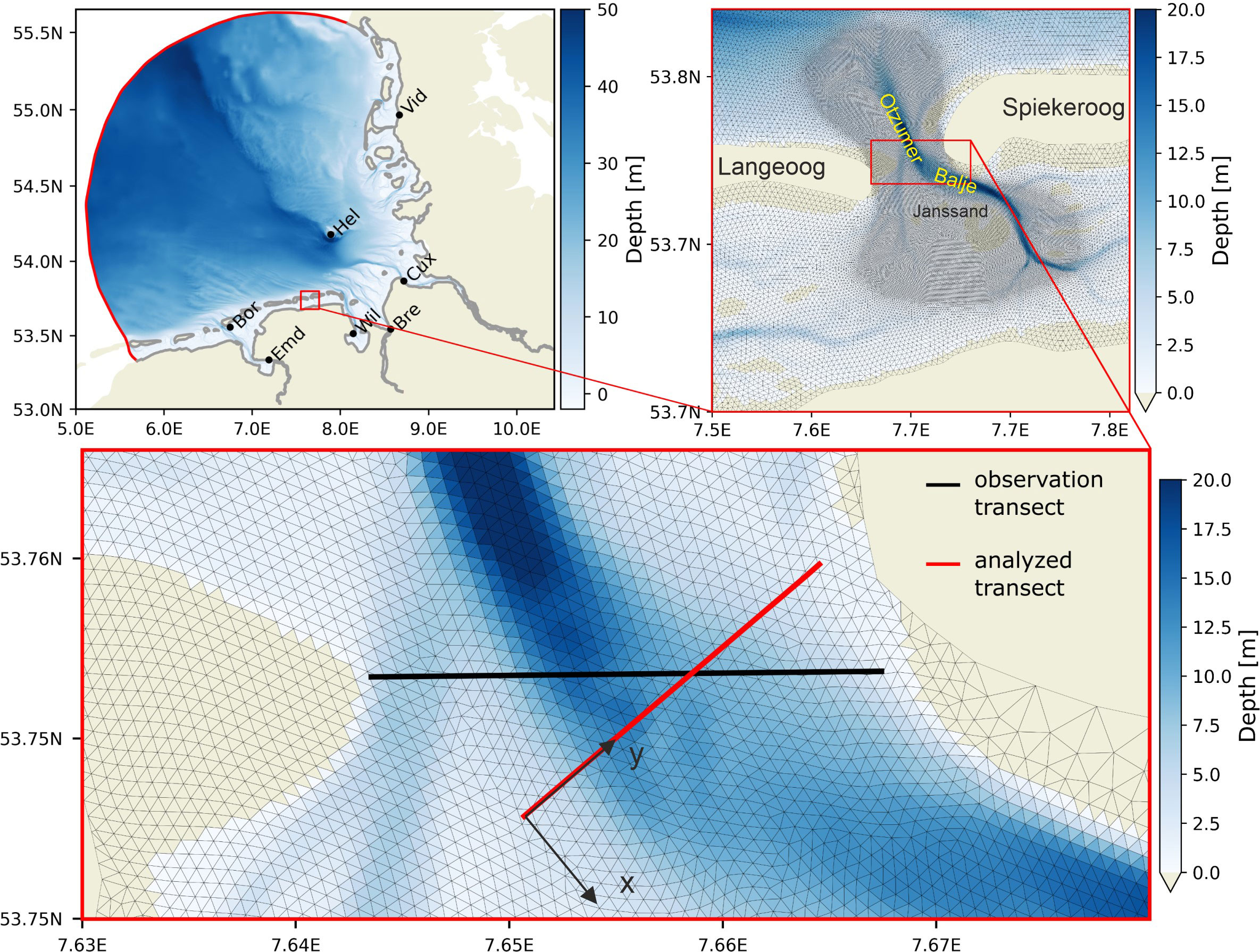
Figure 1 Model domain and bathymetry (left) and the magnified box showing the study site Otzumer Balje (right, red box (left)) and the transect location (bottom, red box (right)). The extent of the oceanward domain is indicated by the red line (left). Black dots depict locations of the tide gauge stations. The increased model resolution in the inlet is indicated by the overlayed mesh (right, the dense region corresponds to 50 m). In the magnified plot of the inlet (bottom); the black line marks the transect sampled by the ADCP, and the red line the orthogonal transect of the channel, along which the secondary circulation is investigated.

Acoustic Doppler current profiler (ADCP) measurements in a cross-section of Otzumer Balje (Valle-Levinson et al. (2018), see their figure 7 are used to validate the numerical model that studies the mechanism responsible for the secondary circulation. The measurements were collected in 2011 along a ~5 km-long transect between Janssand and Spiekeroog (Otzumer Balje, see Figure 1) during neap tide on May 11 and 12 (three tidal cycles), and during spring tide between May 17 and May 19. In total, R/V Otzum traversed the inlet 245 times (136 times during neap tide and 209 times during spring tide), maneuvering at speeds between 2 and 2.5 m s^-1 while a downward-pointing 1200 kHz Teledyne RD Instruments ADCP recorded a velocity profile every 0.8 s. Ensemble averages were taken every 9 profiles, yielding a mean horizontal resolution of ~ m; with a bin size of 0.25 m (Valle-Levinson et al., 2018).

2.2 Model

Hydrodynamic simulations are carried out for the area of the German Bight (Figure 1) from January 1 to July 11, 2011, using the Semi-implicit Cross-scale Hydroscience Integrated System Model (SCHISM) (Zhang et al., 2016), which is a derivative product of the Semi-implicit Eulerian-Lagrangian Finite Element (SELFE) model (Zhang and Baptista, 2008) that solves the Reynolds-averaged Navier–Stokes equations on an unstructured grid under the application of the hydrostatic and Boussinesq approximations. The semi-implicit time step allows numerical stability and efficiency. Moreover, the use of a higher-order Eulerian-Lagrangian method (ELM) to compute the momentum advection reduces constraints on numerical stability. Tracer transport, e.g., salinity, is solved with a 2nd-order total Variation diminishing (TVD) scheme.

The turbulence closure model follows the generic length scale (GLS) formulation of Umlauf and Burchard (2003) as expressed in the k–ϵ parameterization. The parametrization was chosen due to its widespread use and because it was among the most tested closure models. A deeper analysis of the simulated quantities such as turbulent kinetic energy (TKE), dissipation and velocity shears (not shown here) illustrates a reasonable performance. This is further supported indirectly by a suspended sediment modeling study (Stanev et al., 2019), which relies on the performance of the closure model. An important consideration for this study involving the shallow Wadden Sea is the natural treatment of wetting and drying areas. Since most of the Wadden Sea area (such as the tidal basin of the studied channel cross-section) is subject to periodic inundation and drying throughout the tidal cycle, capturing these processes is particularly important for the replication of nonlinear tidal transformations. This was demonstrated in detail by Stanev et al. (2003) for the East Frisian Wadden Sea.

The model setup for the German Bight is based on the model that was presented and validated in Stanev et al. (2019). The mesh size is scaled up to 200 m near the shore of the inlet and the resolution increases up to 50 m in the area inside Otzumer Balje. The horizontal mesh consists of 438k nodes connected within approximately 1 million triangles, while the vertical dimension is resolved with 21 terrain-following sigma coordinates. To facilitate a comparison with the ADCP observations in Otzumer Balje, the model results are mapped from the nodes of the triangular grid cells onto the corresponding transect using inverse distance-weighted horizontal interpolation.

The initial forcing and hydrodynamic open boundary forcing of the German Bight model are interpolated from the 3.6 km Hereon operational Geesthacht Coupled Coastal Model System 35 (GCOAST35)-Nucleus for European Modeling of the Ocean (NEMO) model setup for the northwest European Shelf [for the application and validation of GCOAST, see, e.g., Bonaduce et al. (2020) and Staneva et al. (2021)]. The forcing encompasses sea surface height, three-dimensional velocities, and temperature and salinity at temporal resolutions of one, three, and six hours, respectively.

The atmospheric forcing is derived from the German Weather Service (DWD) Consortium for Small-scale Modeling (COSMO)-Europe (EU) model with an hourly resolution for the atmospheric pressure, 10 m wind, 2 m air temperature, specific humidity and solar radiation (https://opendata.dwd.de/). River discharge is applied for the Ems, Weser and Elbe Rivers from daily observations provided by the German Waterways and Navigation Administration (WSV) (https://www.kuestendaten.de/DE/Startseite/StartseiteKuestendatennode.html). The smaller Eider River is introduced with its annual mean discharge.

2.3 Lateral momentum balance and flow decomposition

To quantify the dominant forcing of the secondary circulation at subtidal timescales, the tidally averaged momentum equation is analyzed in the lateral direction, as has been done in other studies (Geyer, 1993; Lacy and Monismith, 2001; Nidzieko et al., 2008; Zhu et al., 2017; Cui et al., 2018; Chen et al., 2019). In this study, we computed each forcing term for the transect across the tidal inlet (the red line in Figure 1) with the expression given in sigma coordinates (Cheng, 2014):

$\begin{array}{ll}\begin{array}{l}\underset{\text{friction}}{\underbrace{\overline{Z}\frac{\partial }{\partial \sigma }(\overline{A_v}\frac{\partial \overline{v}}{\partial \sigma })}}\underset{\text{local derivative}}{\underbrace{-\frac{\overline{\partial v}}{\partial t}}}\underset{\text{Coriolis}}{\underbrace{-f\overline{u}}}\underset{\text{CFA}}{\underbrace{+\frac{\overline{u^2}}{R}}}\underset{\text{baroclinicity}}{\underbrace{-\frac{g}{{\rho }_0}[\frac{\partial }{\partial y}(\overline{D{\displaystyle {\int }_0^{\sigma }\rho \text{d}\tilde{\sigma }}})+\overline{\rho \sigma \frac{\partial D}{\partial y}}]}}\hfill \\ \underset{\text{advection}}{\underbrace{-(\overline{u\frac{\partial v}{\partial x}}+\overline{v\frac{\partial v}{\partial y}}+\overline{\frac{w}{D}\frac{\partial v}{\partial \sigma }})}}\hfill \\ \underset{\text{ESCO}}{\underbrace{+[\overline{Z}\frac{\partial }{\partial \sigma }(\overline{A_v^{\text{'}}\frac{\partial v^{\prime }}{\partial \sigma }})+\overline{Z^{\prime }\frac{\partial }{\partial \sigma }(A_v^{\text{'}}\frac{\partial v^{\prime }}{\partial \sigma })}+\overline{Z^{\prime }\frac{\partial }{\partial \sigma }(\overline{A_v}\frac{\partial v^{\prime }}{\partial \sigma })}+\overline{Z^{\prime }\frac{\partial }{\partial \sigma }(A_v^{\text{'}}\frac{\partial v^{¯}}{\partial \sigma })}]}}=\underset{\text{barotropic}\text{pres}\text{.}}{\underbrace{g\frac{\partial \overline{\eta }}{\partial y}}}\hfill \end{array}& (1)\end{array}$

Here, the relative depth is σ=(z-η)/D in which D = H + η is the total depth, H is the absolute value of local tidal mean depth and η is the free water surface that deviates from the tidal mean. The variables u and v are the longitudinal (x) and lateral (y) velocity components, respectively, in the σ-coordinates (Figure 1). The positive x-axis is directed in the landward flood direction, the positive y-axis is directed to Spiekeroog, the positive σ-axis is directed upward with the origin at the water surface. The vertical velocity component w(m s^-1) is defined as w = Ddσ/dt with t denoting time. The overbar ($\overline{·}$) and prime (${·}^{\prime }$) denote the tidal mean and tidally varying part of a variable, respectively. Note that $\overline{Z}=1/H^2$ and Z' = 2η/H³ are obtained by estimating 1/D² to the first-order, using Taylor expansion. The Coriolis parameter is f = 10^-4 s^-1, and the gravitational constant of acceleration is g = 9.8 m s^-2. The water density is ρ and has a reference value of ρ₀ = 1000 kg m^-3. In baroclinicity term, $\tilde{\sigma }$ is a dummy variable. The radius of curvature, R was a magnitude of approximately 4 km, with the sign changing from positive (when the bend turns to the positive transverse direction) during flood tide to negative during ebb tide because of the S-shape of the tidal inlet Becherer et al. (2015). The coefficient A_v denotes the vertical eddy viscosity, which is obtained from the k–ϵ model output.

On the left-hand side of Eq. 1, the first term is the friction term. This term is the response of the fluid to the local derivative of inertia, the Coriolis acceleration and other accelerations represented by the remaining terms on the left-hand side of the equation: the centrifugal acceleration (CFA), the baroclinic pressure gradient, nonlinear advection, and eddy viscosity-shear covariance (ESCO). Note that the tidally averaged local acceleration remains in Eq. 1 due to asymmetric tidal currents of flood and ebb. The right-hand side of Eq. 1 represents the barotropic (surface slope-driven) pressure gradient, which balances the terms on the left-hand side of the equation.

The next step is to derive the equations that govern residual currents induced by individual forces. The method follows that of Cheng (2014) and Chen and de Swart (2018), but with a focus on the across-channel direction. The tidally averaged conservation of mass is

$\begin{array}{ll}\frac{\partial }{\partial x}\underset{-1}{\overset{0}{\text{∫}}}\overline{Du}\text{d}\sigma +\frac{\partial }{\partial y}\underset{-1}{\overset{0}{\text{∫}}}\overline{Dv}\text{d}\sigma =0.& (2)\end{array}$

The barotropic residual flow is denoted as ${\overline{v}}_{\text{BT}}$, while the non-barotropic is decomposed into four constituents: the flow due to Coriolis deflection of longitudinal residual current (${\overline{v}}_{\text{C}}$), the baroclinic (density-driven) flow (${\overline{v}}_{\text{D}}$) the ESCO-induced flow (${\overline{v}}_{\text{ESCO}}$) and the advection-induced flow (${\overline{v}}_{\text{ADV}}$). The inertia term is usually negligible (which will be clear in the next section), and thus not included in the non-barotropic constituents. Therefore, the residual currents and the corresponding residual water elevations read

$\begin{array}{ll}\overline{v}={\overline{v}}_{\text{BT}}+{\overline{v}}_{\text{C}}+{\overline{v}}_{\text{D}}+{\overline{v}}_{\text{CFA}}+{\overline{v}}_{\text{ESCO}}+{\overline{v}}_{\text{ADV}},& \text{(3a)}\end{array}$

$\begin{array}{ll}\overline{\eta }={\overline{\eta }}_{\text{BT}}+{\overline{\eta }}_{\text{C}}+{\overline{\eta }}_{\text{D}}+{\overline{\eta }}_{\text{CFA}}+{\overline{\eta }}_{\text{ESCO}}+{\overline{\eta }}_{\text{ADV}}& \text{(3b)}\end{array}$

Substitution of Eq. 3 into Eq. 1 and Eq. 2 yields the equations for the across-channel residual current due to individual forces:

$\begin{array}{ll}\overline{Z}\frac{\partial }{\partial \sigma }(\overline{A_{\nu }}\frac{\partial v_i}{\partial \sigma })-g\frac{\partial {\eta }_i}{\partial y}+F_i=0.& (4)\end{array}$

Here, the subscript i represents an individual component of the residual flow. Integrating Eq. 4 vertically twice and applying zero stress at the free surface and no-slip bottom condition yields

$\begin{array}{ll}{v}_i=\frac{\partial {\eta }_i}{\partial y}{p}_1-p_i,& (5)\end{array}$

with

$\begin{array}{ll}{p}_1=\frac{g}{\overline{Z}}{\displaystyle {\int }_{-1}^0\frac{\sigma }{\overline{A_{\nu }}}\text{d}\sigma .}& (6)\end{array}$

In the across-channel direction, it is considered that the net water transports are barotropic, i.e., F_BT=0. Thus, integrating Eq. 2 across the section from the side boundary (–B) yields the barotropic transport, which can be computed numerically from the model output:

$\begin{array}{ll}{\displaystyle {\int }_{-1}^{0}H{\overline{v}}_{\text{BT}}\text{d}\sigma =-\frac{\partial }{\partial x}{\displaystyle {\int }_{-B}^y{\displaystyle {\int }_{-1}^0\overline{Dud}\sigma \text{d}y+}}}{\displaystyle {\int }_{-1}^0\overline{Dvd}\sigma {|}_{y=-B}}={\displaystyle {\int }_{-1}^{0}H{\overline{v}}^{*}\text{d}\sigma ,}& (7)\end{array}$

where ${\overline{v}}^{*}$ is the tidally averaged across-channel velocity prescribed from the model at each grid point. Substitution of Eq. 5 into Eq. 7 yields the lateral barotropic water-level slope

$\begin{array}{ll}\frac{\partial {\eta }_{BT}}{\partial y}={\displaystyle {\int }_{-1}^{0}H{\overline{v}}^{*}\text{d}\sigma /{\displaystyle {\int }_{-1}^{0}H{p}_1\text{d}\sigma .}}& (8)\end{array}$

Considering that the ratio of width to length of the tidal inlet (Figure 1) is small, the continuity equation regarding flow components due to non-barotropic forces is simplified as (Cheng, 2014)

$\begin{array}{ll}{\displaystyle {\int }_{-1}^{0}H{\overline{v}}_i\text{d}\sigma =0.}& (9)\end{array}$

Hence, applying boundary conditions at the surface and the bottom to the corresponding reduced momentum equations (Eq. 4) and the continuity equations (Eq. 9), the expressions p_i corresponding to Coriolis (“C”), density gradient (“D”), curvature (“CFA”), ESCO mechanism (“ESCO”) and the advection (“ADV”) are

$\begin{array}{ll}{p}_{\text{C}}=\frac{1}{\overline{Z}}{\displaystyle {\int }_{-1}^{\sigma }\frac{{\displaystyle {\int }_{\tilde{\sigma }}^0<f\overline{u}>\text{d}{\tilde{\sigma }}_1}}{\overline{A_v}}}\text{d}\tilde{\sigma }& \text{(10a)}\end{array}$

$\begin{array}{ll}{p}_{\text{D}}=\frac{1}{\overline{Z}}{\displaystyle {\int }_{-1}^{\sigma }\frac{{\displaystyle {\int }_{\tilde{\sigma }}^0\frac{g}{{\rho }_0}\langle \frac{\partial }{{\partial }_y}(D{\displaystyle {\int }_{{\tilde{\sigma }}_1}^0\rho d{\tilde{\sigma }}_2})+\overline{\rho {\tilde{\sigma }}_1\frac{\partial D}{\partial v}}\rangle }d{\tilde{\sigma }}_1}{\overline{A_v}}}d\tilde{\sigma }& \text{(10b)}\end{array}$

$\begin{array}{ll}{p}_{\text{CFA}}=-\frac{1}{Z}{\displaystyle {\int }_{-1}^0\frac{1}{\overline{A_v}}{\displaystyle {\int }_{\tilde{\sigma }}^0<\frac{\overline{u{\text{'}}^2}}{R}>}}\text{d}{\tilde{\sigma }}_1\text{d}\tilde{\sigma }& \text{(10c)}\end{array}$

$\begin{array}{ll}\begin{array}{l}{p}_{\text{ESCO}}={\displaystyle {\int }_{-1}^{\sigma }\frac{1}{\overline{A_v}}}\langle A_v^{\text{'}}\frac{\partial \overline{v}}{\partial {\tilde{\sigma }}_1}\rangle d\tilde{\sigma }-{\displaystyle {\int }_{-1}^{\sigma }\frac{1}{\overline{A_v}}}{\displaystyle {\int }_{\tilde{\sigma }}^0\langle \overline{\frac{Z^{\prime }}{\overline{Z}}\frac{\partial }{\partial {\tilde{\sigma }}_1}(A_v^{\text{'}}\frac{\partial \overline{v}}{\partial {\tilde{\sigma }}_1})}\rangle }d{\tilde{\sigma }}_{1}d\tilde{\sigma }-\\ {\displaystyle {\int }_{-1}^{\sigma }\frac{1}{\overline{A_v}}}{\displaystyle {\int }_{\tilde{\sigma }}^0\langle \overline{\frac{Z^{\prime }}{\overline{Z}}\frac{\partial }{\partial {\tilde{\sigma }}_1}(\overline{A_v}\frac{\partial v^{\prime }}{\partial {\tilde{\sigma }}_1})}\rangle }d{\tilde{\sigma }}_{1}d\tilde{\sigma }-{\displaystyle {\int }_{-1}^0\frac{1}{\overline{A_v}}{\displaystyle {\int }_{\tilde{\sigma }}^0\langle \overline{\frac{Z^{\prime }}{\overline{Z}}\frac{\partial }{\partial {\tilde{\sigma }}_1}(A_v^{\text{'}}\frac{\partial \overline{v}}{\partial {\tilde{\sigma }}_1})}\rangle }}d{\tilde{\sigma }}_{1}d\tilde{\sigma }\end{array}& \text{(10d)}\end{array}$

$\begin{array}{ll}{p}_{\text{ADV}}=\frac{1}{\overline{Z}}{\displaystyle {\int }_{-1}^{\sigma }\frac{1}{\overline{A_v}}{\displaystyle {\int }_{\tilde{\sigma }}^0\langle \overline{u\frac{\partial v}{\partial x}}+\overline{v\frac{\partial v}{\partial y}}+\overline{\frac{w}{D}\frac{\partial v}{\partial {\tilde{\sigma }}_1}}\rangle }}d{\tilde{\sigma }}_{1}d\tilde{\sigma }& \text{(10e)}\end{array}$

where "< · >" denotes taking vertical variation of the forces.

3 Results

3.1 Model validation

The model has been extensively validated in Stanev et al. (2019) at the scale of the German Bight. Hence for the model validation, the observation transect (see Figure 1 for the location) is taken to compare the modeled residual currents with observations. As shown in Figure 2, the spatial patterns of the observed streamwise residual current are well represented by the model. In both neap tide and spring tide, the residual current is inward (from the North Sea to the Wadden Sea) with a maximum of 6 cm s^-1 in the middle of the transect and outward near the edge of the western and eastern shoals. The direction change occurs at approximately 0.4 km and 0.9 km from the western boundary. However, differences exist between measurements and the simulation. The maximum inflow is observed inside the water column near the deep trough of the channel, at ~0.7 m from the western boundary, while the model predicts the maximum current at the water surface near ~0.5 m. Moreover, the model overestimates the outflow, especially over the western shoal from 0 to 0.3 km.

FIGURE 2

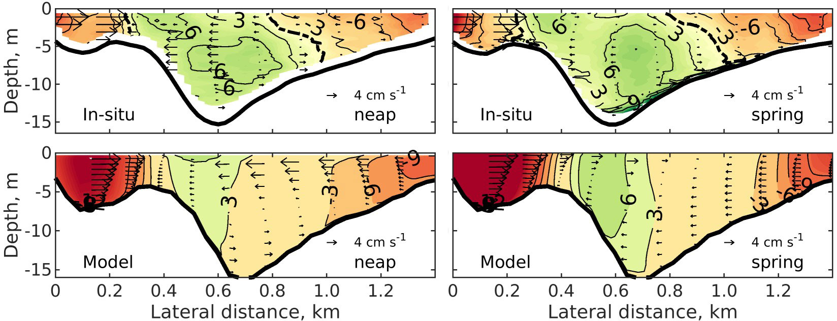
Figure 2 (In-situ) measured and (model) simulated residual currents at neap and spring tides along the observed transect. Here, in-situ measurements are adapted from Figure 7 of Valle-Levinson et al. (2018). Contours denote longitudinal currents that are perpendicular to the transect and arrows represent the lateral currents. In the longitudinal direction, positive values (in green contours) indicate inflow (when looking seaward). Units of the currents are cm s⁻¹. Dashed lines illustrate the 0 cm s⁻¹ longitudinal current contours.

For the lateral component, the model is able to represent major features of the observations of the transect. In neap tide, a two-layer current is observed in the main channel of the transect, i.e., the lateral distance between 0.6 km and 1.0 km (Figure 2). The lateral flow is mainly to the left (looking seaward) at 0.6 km, showing a maximum in the middle of the water column. Leftward flow converges with rightward flow at approximately 0.3 km (Figure 2, upper left), where the longitudinal current reverses direction. In spring tide, convergence of lateral flow is found at the same place. However, east of this location, from 0.3 to 1.0 km, the surface lateral flow reverses to rightward. These features are captured by the model. Regarding model-data differences, in neap tide model shows a larger leftward current near the surface of the right side of the transect (0.6~1.4). The observed leftward currents are 2~3 m s^-1 while the model flows are 4 ∼ 6 cm s^-1. During spring tide, the modeled rightward current near the water surface is larger than the in-situ data and extends deeper in the water column. The measurement shows a rightward current with a magnitude of 1 - 2 cm s^-1 hear the bed on the right shoal (0.8 ~ 0 km), while the modeled current is leftward. Moreover, the currents over the slope near the right-hand boundary (1.0 ~ 0.4 km) are overestimated by the model.

Considering the subtidal secondary circulation is on a scale of 2~3 m s^-1 validating the model performance in the cross-channel plain is a challenge. Minor errors in, e.g., bathymetry and measured velocities, may cause differences. Despite the model and observations differences, the basic patterns in both neap and spring tides remain similar. This comparison demonstrates the reliability of the model to study lateral dynamics over the “analyzed transect” (the red transect in Figure 1), which maximized the longitudinal flows following the principal axis (perpendicular to the “analyzed transect”).

3.2 Stratification and secondary circulation

To quantify the degree of stratification, the potential energy anomaly (Θ) is computed across the analyzed transect:

$\begin{array}{ll}\text{Θ}=D\underset{-1}{\overset{0}{\int }}g\sigma (\widehat{\rho }-\rho )\text{d}\sigma ,& (11)\end{array}$

where $\widehat{\rho }$ denotes the vertical mean water density. Figure 3 suggested that destratification is stronger during spring tide than during neap tide. Stratification is strongest at the end of neap ebb tide. During spring tide, the water column is mostly well-mixed. A short period of stratification is observed (with Θ being approximately 1~5 J m^-3 toward the end of flood, when the cross-channel current is close to zero at high water. The late flood straining observed in the model is consistent with that reported by Becherer et al. (2015), who applied a time-dependent dynamic equation to the potential energy anomaly (Burchard and Hofmeister, 2008). The overall stratification at the Otzumer Balje inlet transect is weak, with a maximum Θ of 4 J m^-3 during neap tide and a maximum of 2 J m^-3 during spring tide.

FIGURE 3

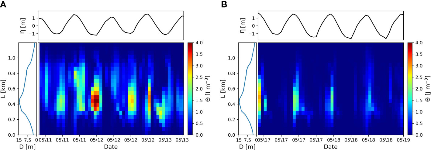
Figure 3 Potential energy anomaly (Θ) over time and along the transect during the neap (A) and spring (B) tides. Curves on top show the tidal elevation (η) in the center of the transect (black). The axis to the left shows the depth (D) along the lateral distance (L) of the transect.

Figure 4 shows the along- and cross-channel transect velocities on the analyzed transect at four phases of a tidal cycle during neap and spring tides. The largest along-channel tidal currents (the peaks of both flood tide and ebb tide) occur at the surface on the right side (looking seaward) of the thalweg. Phase differences are also observed between the currents at shoals and those in the deep channel (e.g., end of the ebb and flood during neap tide), as well as at the surface and bottom (end of the flood tide during spring tide).

Different spatial patterns arise in the cross-channel flow at different tidal stages from neap to spring tides. For example, at the end of ebb during neap tide, a two-layer secondary flow develops in the deep channel, with currents directed toward the left shoal near the surface and a return flow at the bottom (Figure 4A). At peak flood, the tidal current diverges at approximately 0.45 km (Figure 4B). On the right shoal the maximum cross-channel current is located near the bottom and decreases toward the surface. At the end of the flood tide, the current near the surface of the right shoal reverses, while the current in the lower layers remain toward the right (Figure 4C). A anti-clockwise rotation develops akin to that at the end of ebb tide. Later, in the ebb phase, the tidal current flows from the left side (looking seaward) and converges with the leftward current from the right shoal at 0.45 km. The current structure at the ebb peak reverses compared to that at the flood peak (Figure 4D).

FIGURE 4

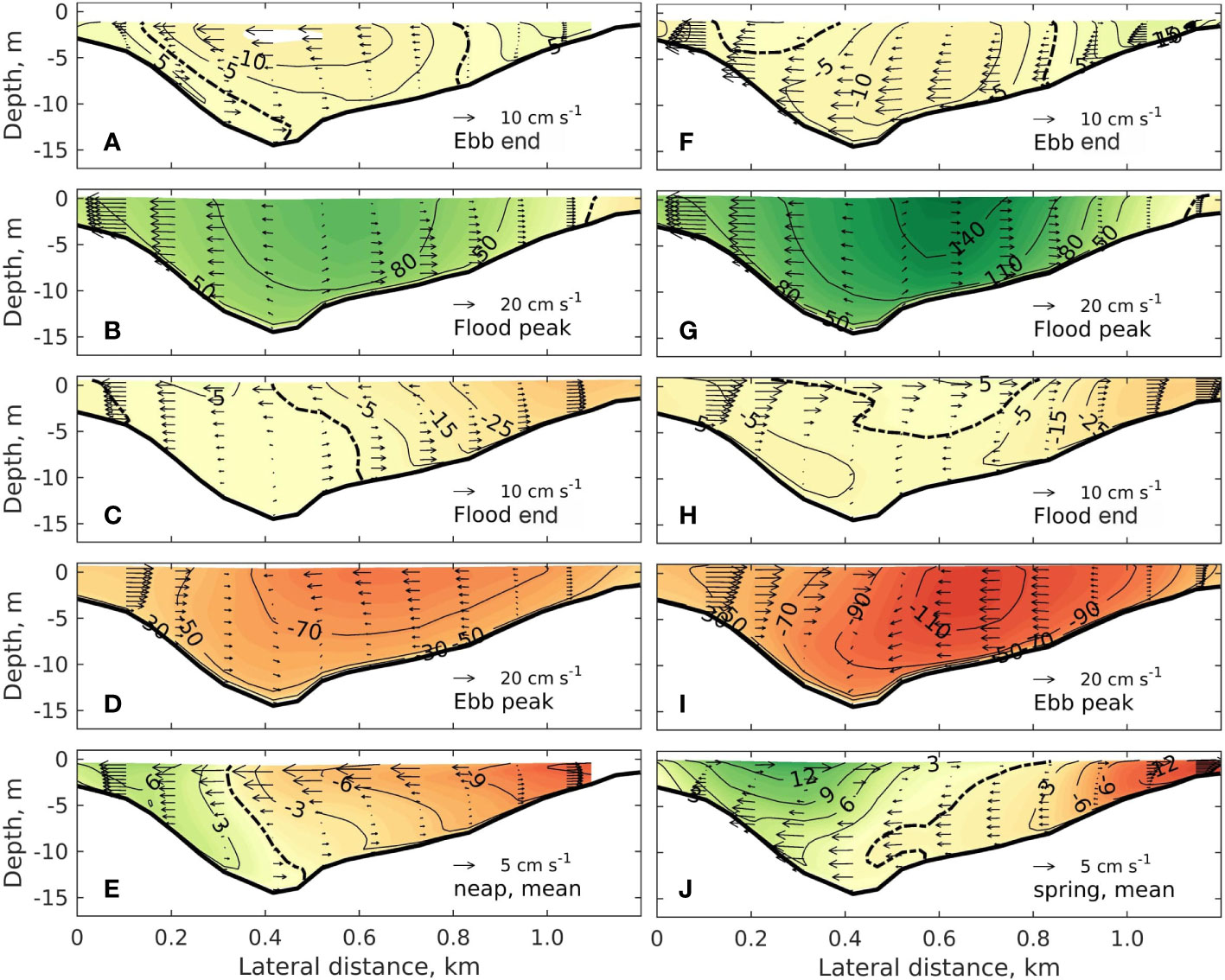
Figure 4 Transverse distributions (looking seaward) of the currents in along-channel (contours, the green colors are flowing toward the viewer) and cross-channel (arrows) directions at different phases of the neap (left column) and spring (right column) tides. The first to the fourth rows show the end of ebb (the cross-sectional mean of the along-channel ebb flow is zero) (A, F), the flood peak (the cross-sectional mean of the along-channel flood flow is the maximum) (B, G), the end of flood (cross-sectional mean along-channel flood flow is zero) (C, H) and the ebb peak (cross-sectional mean along-channel ebb flow is maximum). (D, I) The fifth row shows the tidal mean. (E, J) Thick dashed curves indicate the 0 m s⁻¹ contours.

The cross-channel current pattern during spring tide is similar to that during neap tide at the flood and ebb peaks (Figures 4G, I, comparing with b and d), but the velocities are larger during spring tide due to the stronger external tidal forcing. Spring-tide flood and ebb ends, however, show distinct structures compared to that during neap tide. At the end of ebb tide, a leftward current is observed across the transect as the velocity increases toward the bottom (Figure 4F). At the end of the flood tide, a two-layer flow appears with the opposite sign to that observed during neap tide (Figure 4H).

During both tidal periods, the along-channel residual current consists of inflow along the left side of the channel and outflow on the right side (Figures 4E, J). In the cross-channel direction, the residual currents show a two-layer structure both in the neap and spring tides, but with opposite signs. Considering that the inlet is predominately well-mixed, the lateral density gradient generated by differential advection is weak. The density difference over the entire cross-section has a magnitude of ~10^-2 g m³ in both neap and spring tide. Further analysis reveals that in both periods, the leftward current is much larger than the rightward current. The difference is that during neap tide, the strong leftward current is near the surface while in spring tide it is close to the bottom. Integrating lateral residual currents over the entire water column yields a net water transport from the right shoal to the left shoal for both neap and spring tides (not shown).

3.3 Momentum balance

The individual terms of the residual lateral momentum budget (see Eq. 1) are computed on the transect analyzed (see Figure 1). Figure 5 compares the depth-averaged acceleration terms with the barotropic pressure gradient. In both neap and spring tides, the sum of all accelerations (left-hand side of Eq. 1) approximately equals the barotropic pressure gradient (right-hand side of Eq. 1) along the transect. Advection is dominant on the vertically averaged subtidal momentum budget, implying a small contribution to the net transverse transport due to the other accelerations. This result is consistent with the assumptions made for the decomposition method in the previous section. Differences between the sum and the barotropic pressure gradient are caused mainly by numerical errors from interpolating the model output to the grids on the transect analyzed.

FIGURE 5

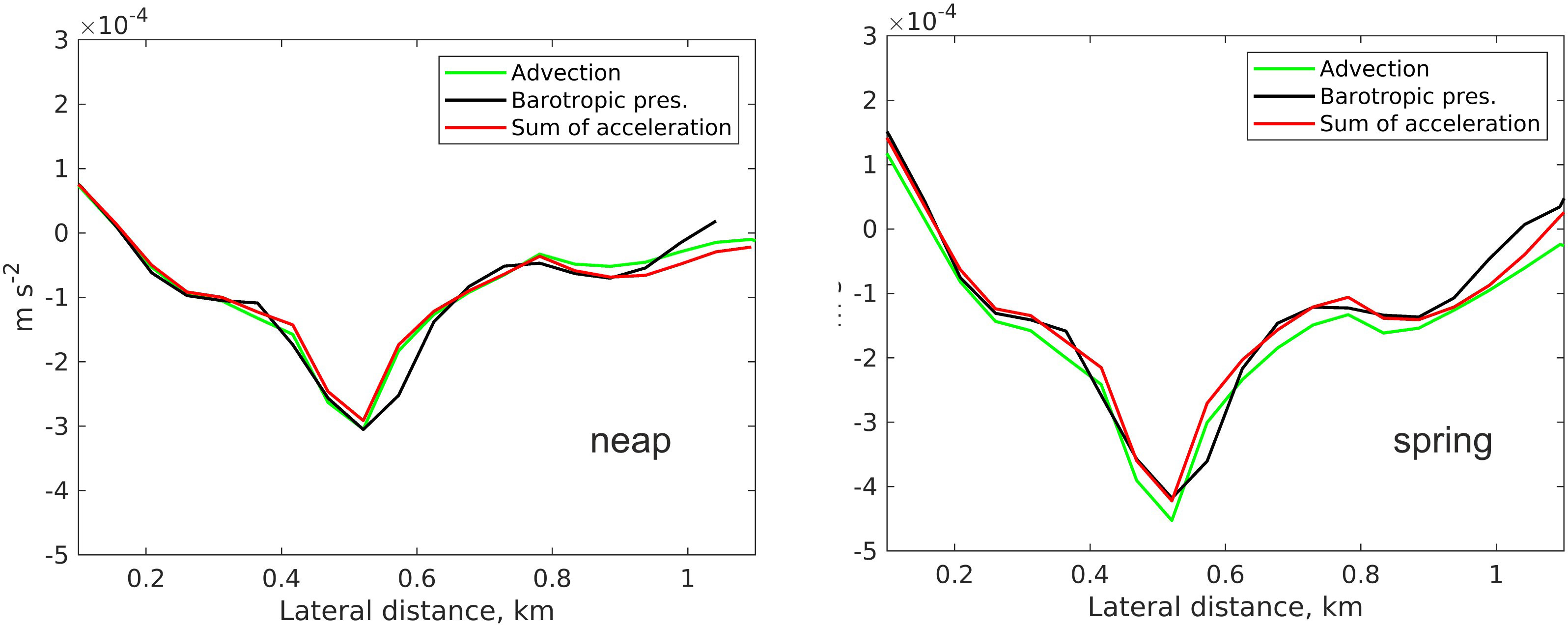
Figure 5 Vertical average of the forcing terms of the subtidal lateral momentum balance along the analyzed transect in (left) neap and (right) spring tide.

Individual acceleration terms of the momentum budget as a function of depth and position, are shown in Figure 6. During neap tide, the local derivative (inertia) is the smallest term among all contributions to the residual lateral momentum budget. The baroclinic pressure gradient induces clockwise accelerations (looking seaward) on the slopes and anti-clockwise accelerations over the main channel (Figure 6B). The contribution of baroclinicity reaches a value of ±1 × 10⁻⁵ m s^-2, which is one order of magnitude larger than the Coriolis accelerations (Figure 6C). The ESCO mechanism shows a three-layer structure, with leftward accelerations both near the surface and bottom, and a rightward acceleration in between. The ESCO magnitude is as large as that from the baroclinic pressure gradient (Figure 6D). The CFA is clockwise on the left slope, while it is anti-clockwise in the thalweg and the right slope (Figure 6E). In comparison, lateral advection dominates the contributions to the depth-dependent lateral momentum budget (Figure 6F).

During spring tide, the local derivative remains small (Figure 6I). The lateral baroclinic pressure gradients drive clockwise-rotating accelerations over the main channel and the left slope, and a relatively small anti-clockwise rotation on the right slope (Figure 6J). The Coriolis acceleration is comparable to the baroclinicity but shows a single rotating cell directed toward the left near the surface and toward the right near the bottom (Figure 6K). The ESCO mechanism causes a single rotating cell (Figure 6L), in which the acceleration is from left to right near the surface and to the right underneath. Its contribution to the momentum budget is much larger than that of baroclinicity (Figure 6J). This result reveals that the ESCO mechanism is more relevant than the baroclinicity in predominantly well-mixed coastal waters. This finding is similar to that of Cheng et al. (2013), who focused on the along-channel direction. Remarkably, compared to the neap tide, CFA reverses in the thalweg and the right slope (Figure 6M). It is smaller than the ESCO but has a similar spatial structure. In spring tide, advection is similar to that of the neap tide, regarding both the spatial pattern and the magnitude, except for the near-surface layers of the deep channel.

The sum of the individual acceleration terms (Figures 6G, O) is equivalent to the ‘Friction’ (with a minus sign) (Figures 6H, P). With a perfect model performance and momentum budget decomposition, the ‘Sum’ and the negative ‘Friction’ terms should be identical (in balance). Overall, the differences in this application are small.

3.4 Residual flow components

Figure 7 further shows the spatial structure of the cross-channel residual flow induced by the individual accelerations displayed in Figure 6. The barotropic flow v_BT. (Figures 7A, I) and the flow induced by the non-barotropic part of advection, v_ADV (Figures 7F, N), are dominant residual components. They reach more than ~4 m s^-1. The barotropic flow diverges at 0.7 km in neap tide and at 1 km in spring tide. It also shows a convergence at the left shoal during spring tide. The baroclinic flow and the Coriolis flow are mostly less than 0.3 cm s^-1 except for v_D in the main channel, where it reaches 1 cm s^-1 The difference between the two tidal periods is that the ESCO flow v_ESCO changes the spatial structure and becomes more important from neap to spring tide. Over the left side of the deep channel (0.4 km), the ESCO flow direction reverses (Figures 7D, K). The maximum velocity exceeds 3 m s^-1 but the surface in spring tide. In neap tide, the CFA-induced flow is similar to that driven by advection, but with a small magnitude. The CFA-induced flow reverses its direction over the thalweg and the right slope during the spring tide. The flow is rightward near the surface and leftward near the bottom, which is similar to the two-layer structure of the ESCO flow, but with a magnitude of approximately 50% lower. Summing all individual residual flow components yields flow with spatial patterns (Figures 7G, O) similar to that obtained by averaging the modeled lateral flow in tidal periods (Figures 7H, P), demonstrating a valid performance of the decomposition method.

FIGURE 6

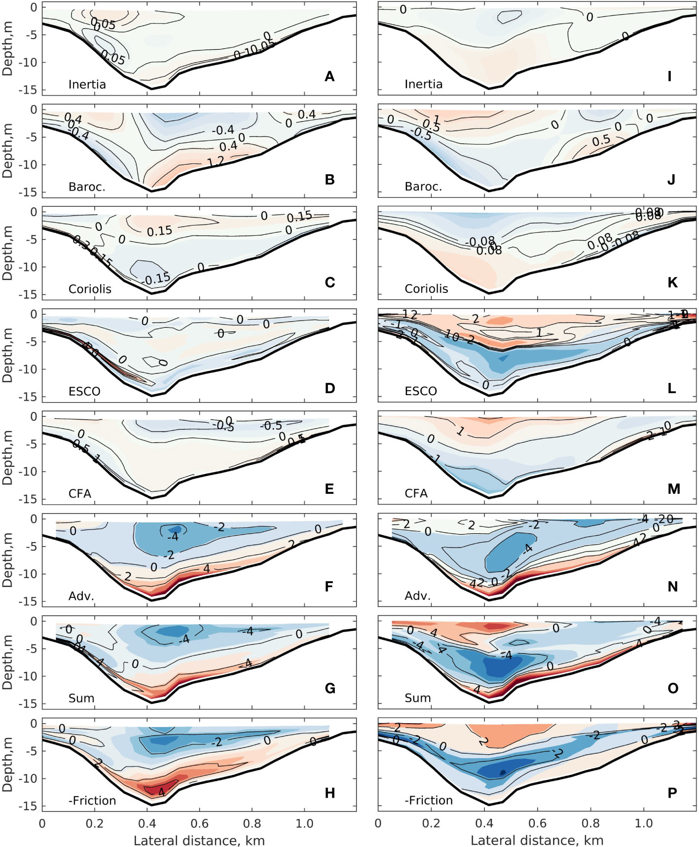
Figure 6 Transverse distributions of the individual terms of the subtidal lateral momentum balance during (left column) neap tide and (right column) spring tide: (A, I) local derivative inertia, (B, J) baroclinicity (Baroc.), (C, K) Coriolis, (D, L) ESCO and (E, M) CFA, (F, N) nonlinear advection (ADV). (G, O) are the summation of the above terms. To compare with the summation, (H, P) show the friction term with a minus sign. All terms have the vertical mean removed. Positive values indicate rightward momentum tendency. The unit in all contours is ×10⁻⁵ m s⁻².

The lateral residual flow due to advection, i.e., the summation of the barotropic part v_BT (Figures 7A, I) and the non-barotropic part v_ADV (Figures 7F, N), is shown in Figure 8. It has a comparable structure and magnitude as the v_m in the neap tide, revealing its dominance in subtidal secondary circulation. In spring tide, the flow driven by advection presents a similar structure as that during the neap tide, e.g., currents leftward near 0.1 km and rightward near 1.1 km with a velocity of approximately 4 cm s^-1. Moreover, between 0.3 km and 0.9 km the flow is leftward near the surface and rightward near the bottom, despite the difference in flow intensity (4 cm s^-1 n neap tide and 2 cm s^-1 in spring tide). This implies that the change in advective process from neap to spring tide is small.

FIGURE 7

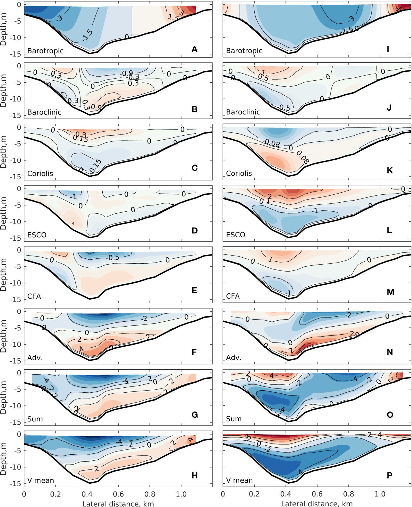
Figure 7 Transverse distributions of the across-channel residual flow due to individual terms of the subtidal lateral momentum balance during (left column) neap tide and (right column) spring tide: (A, I) barotropic flow (v_Baro), (B, J) baroclinic (density-driven) flow (v_D), (C, K) flow due to Coriolis deflection (v_C), (D, L) ESCO induced flow (v_ESCO), (E, M) CFA induced flow,V_CFA and (F, N) nonlinear advection (v_ADV). Panels (G, O) are the summation of the above terms. Panels (H, P) show the tidal mean velocity. Positive values indicate rightward flow. The unit in all contours is cm s⁻¹.

FIGURE 8

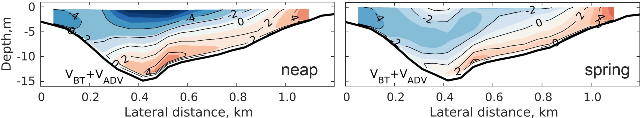
Figure 8 Transverse distributions of the across-channel residual flow due to advection (the sum of v_Baro and v_ADV) during (left column) neap tide and (right column) spring tide. The unit in all contours is cm s⁻¹.

Comparing the advective flow with the mean flow (v_m) clearly demonstrates the contribution of the ESCO mechanism. The clockwise circulation induced by ESCO acts against advection and reverses the lateral flow near the surface (Figure 7O). Meanwhile, the ESCO flow below the surface enhances the leftward flow. The baroclinic flow (v_D) as a pattern similar to that of the ESCO flow but with a magnitude 2~3 times smaller (Figure 7I). The CFA also plays a role in subtidal secondary circulation, especially during spring tide, which together with ESCO, contributes to the reversal of the subtidal secondary circulation. The analysis reveals that the reversal of the flow due to the ESCO mechanism (Figures 7D, K) plays the most important role in the change of the subtidal secondary circulation pattern between neap and spring tide (Figures 7H, P).

The decomposition analysis is also applied to the observation transect (the black line in Figure 6), where the barotropic transport is mainly driven by the advection and could be isolated from the other processes. On the depth-dependent momentum budget, the advection also plays a dominant role for both neap and spring tides. However, similar to the findings on the transect analyzed, the ESCO mechanism explains the clockwise circulation observed at 0.5 km of the observation transect during spring tide (see Figure 2). Figures illustrating structures of the decomposed flow are provided in the Supplementary Material.

3.5 ESCO mechanism

To understand the changes in the ESCO-induced acceleration, as well as the flow, from neap tide to spring tide, the ESCO mechanism is further scrutinized. The ESCO mechanism (see Eq. 1) consists of four covariance components, namely, those between the tidal velocity (v'), tidal elevation ($\overline{Z}$) and the tidally varying component of the eddy viscosity ($A_v^{\prime }$). Note that $A_v^{\prime }$ changes with respect to the tidal mean, and is negative when turbulent mixing is relatively weak in the tidal cycle. To quantify the contributions of different covariances to the ESCO mechanism, each term is computed separately. The ESCO acceleration mainly results from the first term (not shown), i.e., the covariance between the tidally varying part of the eddy viscosity ($A_v^{\prime }$) and the vertical shear of the lateral tidal velocity ($\partial v/\partial \sigma$). The contributions of the other terms are one order of magnitude smaller.

Given the complexity of the correlations in ESCO, the structures of $\partial v/\partial \sigma$ and $A_v^{\text{'}}$ it different phases of a tidal cycle are analyzed for both neap and spring tides. Figure 9 shows ∂v/∂σ, $A_v^{\text{'}}$ and their product $A_v^{\text{'}}\frac{\partial v}{\partial \sigma }$ at four phases of the neap tide: end of the ebb, peak flood, end of flood and peak ebb. Because the tidal mean of the eddy viscosity is removed, negative values of $A_v^{\prime }$ indicate a smaller eddy viscosity value than the tidal mean. This occurs from late ebb to early flood and from late flood to early ebb. At the end of the ebb tide, the velocity shear exhibits a structure with values of opposite signs with respect to the deep channel, which, when multiplied with a negative $A_v^{\text{'}}$ for the entire cross-section, yields $A_v^{\prime }$$\frac{\partial v}{\partial \sigma }$ with a similar structure as the shear. At flood peak, the $\partial v/\partial \sigma$ values change signs over the left shoal and the upper layer of the right shoal, meanwhile $A_v^{\text{'}}$ becomes positive. Their product again yields a cross-sectional pattern similar to that of end of ebb. At the end of flood, the vertical shear has two-layer structures but displays opposite signs over the two shoals. A similar feature is observed in $A_v^{\text{'}}$ with respect to the deep channel, with values of different signs. This leads to a three-layer structure of $A_v^{\text{'}}\frac{\partial v}{\partial \sigma }$ over the two shoals, despite a relatively weaker product compared to the other phases. At maximum ebb, $A_v^{\text{'}}$ has a two layer structure on the right shoal and the deep channel, with positive values in deep water columns and negative at the surface. Over the left shoal, $A_v^{\text{'}}$ is mostly negative (except for the section close to the left side boundary). The spatial structure of the vertical shear at this phase is negative over the right shoal and positive over the left shoal. The product of $A_v^{\text{'}}\frac{\partial v}{\partial \sigma }$ reflects similar features as $\partial v/\partial \sigma$. The residual $A_v^{\text{'}}\frac{\partial v}{\partial \sigma }$ bottom plot of Figure 9) has a two-layer pattern on the right shoal and the channel, while it is almost three layers over the right shoal.

A similar analysis is made for spring tide (Figure 10). Both the cross-sectional distribution and the magnitude of $A_v^{\text{'}}$ it different tidal phases are similar to those at neap tide. The only difference occurs at flood slack, when $A_v^{\text{'}}$ is negative along the entire cross-section. However, $A_v^{\text{'}}\frac{\partial v}{\partial \sigma }$ during spring tide shows a pattern rather different compared to that during neap tide. It is negative over almost the entire tidal cycle. This is because the velocity shear has patterns that are different from those at neap tide. For example, $\partial v/\partial \sigma$ is mostly positive at the end of ebb while it becomes negative throughout the section near the flood peak. This pattern suggests that the maximum lateral velocity is near the bottom and decreases toward the surface. A similar situation occurs near peak ebb. The velocity shear is negative from the thalweg to the right shoal, where $A_v^{\text{'}}$ is positive. On the left shoal, the eddy viscosity is still smaller than the tidal mean and the vertical shear remains positive. As a result, the product retains the same sign. Taking an average over the tidal cycle yields a negative value of the product.

4 Discussion

Processes related to the turbulent fluxes of momentum have been highlighted by many studies, with a focus on the along-estuary direction; these processes included the asymmetries in tidal turbulence between flood and ebb due to the strain-induced periodic stratification (Simpson et al., 1990; Jay and Musiak, 1994; Geyer et al., 2000), bottom friction (Li and Zhong, 2009; Ross et al., 2019), lateral processes (Basdurak et al., 2017) and quarter-diurnal tides (Dijkstra et al., 2017). Following these frameworks, quantifying the variable ESCO circulation pattern mainly involves the intensity and the phase of asymmetries in tidal turbulence mixing regarding flood and ebb tides (Stacey et al., 2008; Burchard and Hetland, 2010; Cheng et al., 2010; Burchard et al., 2011). The phase is affected by the strength of water column stratification. For instance, Cheng et al. (2013) and Chen and de Swart (2018) investigated an idealized estuarine channel, and the flood/ebb directions were restricted to a uniform streamwise direction during both spring and neap tides. Hence, the difference in the ESCO structure has been attributed to a change in the shape of the eddy viscosity profile. This profile shows a maximum value shifting from the middle of the water column to the bottom when stratification increases. Moreover, the relative importance of the ESCO flow decreases from being dominant in periodical stratification to negligible in a highly stratified water column relative to the density-driven flow.

The fundamental mechanism is that the tidally averaged longitudinal momentum tendency is generated by stratification and destratification of the water columns within tidal cycles, which results from the straining of the horizontal density gradient (MacCready and Geyer, 2010; Geyer and MacCready, 2014). The results shown in the present work, however, are distinct from those of other studies, with the focus on the ESCO mechanism responsible for the secondary circulation. The Otzumer Balje tidal inlet is predominantly well-mixed and the change in stratification is small from neap to spring tide (see Figure 3). In both tidal regimes, the tidally averaged eddy viscosity has a similar magnitude and presents a similar structure over the cross-section: a parabolic profile in the vertical direction with a maximum value (∼ 0.03 m² s⁻¹ in deep channel) in the middle of the water column. The gradient Richardson number is less than 0.25 for the whole period during both spring and neap tides (not shown), indicating small asymmetries in turbulent mixing from flood to ebb.

The change in the ESCO structure from neap tide to spring tide is caused primarily by the difference in the vertical shear in the lateral flow (Figures 9, 10). To further understand this difference, Figure 11 illustrates the lateral tidal currents (v') during neap and spring tides. During the neap tide, the lateral tidal flow increases from the bottom to the surface, with the maximum velocity (both ebb and flood) appearing at the surface. However, during spring tide, for both ebb and flood phases the lateral tidal flow has a maximum near the bottom on the right side shoal. This illustration demonstrates the current veering from the bottom to the surface. Compared to the neap tide, the spring tide ebb currents veer to the right from the bottom to the surface. In contrast, the flood currents rotate leftward. Although the speed of the tidal current (e.g., the flood current) decreases from the surface to the bottom, its projection in the cross-channel direction (the positive direction is from the left bank toward the right) increases downward.

FIGURE 9

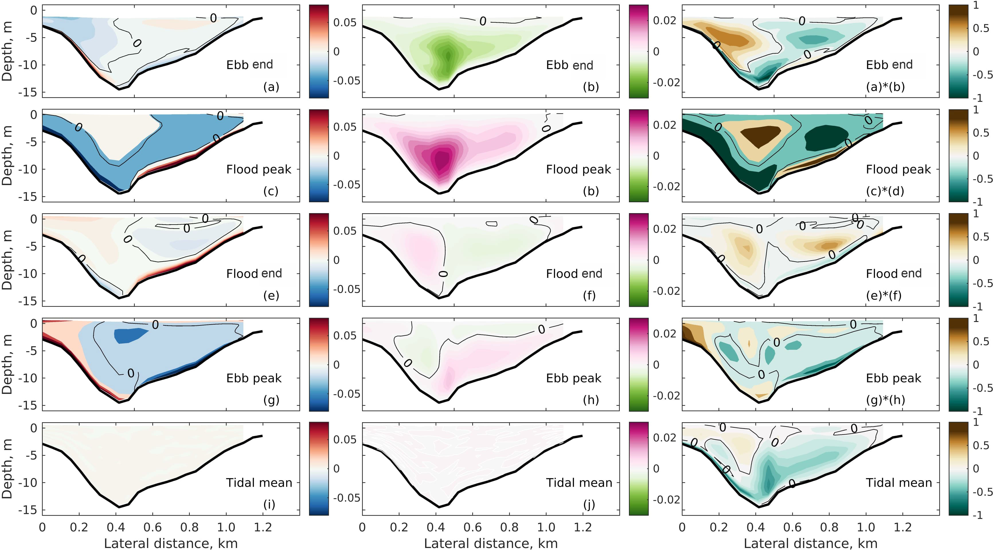
Figure 9 Transverse distributions of (first column) the vertical shear (∂v/∂σ, m s⁻¹), (second column) the tidally varying eddy viscosity $(A_v^{\text{'}},{\text{m}}^2{\text{s}}^{-1})$ and the product $A_v^{\text{'}}\frac{\partial v}{\partial \sigma }$ at different phases of the neap tide. All plots are looking seaward.

FIGURE 10

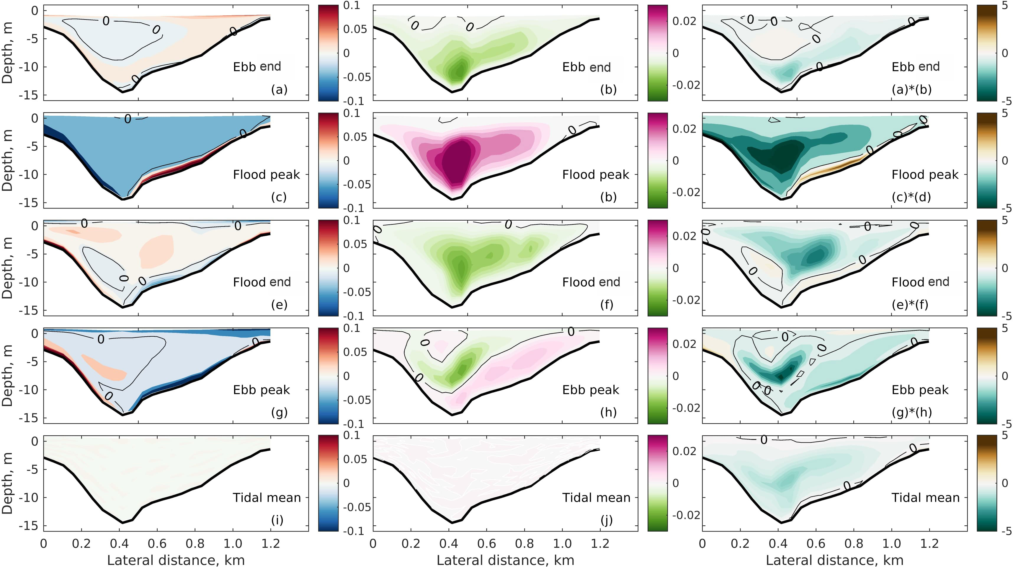
Figure 10 Same as for Figure 9, but for spring tide.

FIGURE 11

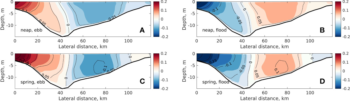
Figure 11 Lateral tidal flow for (upper panels) the neap tide and (lower panels) the spring tide. The left column plots (A, C) and the right column plots (B, D) are the time mean currents for the ebb and food, respectively. All plots are with the tidal residual component removed.

Several factors related to a curving channel can influence the vertical shear of the cross-channel currents. For example, asymmetric bedforms yield an asymmetric bottom stress distribution (Fong et al., 2009). Other factors include the channel slope, radius of curvature, and channel-shoal combination, where the last factor causes the interaction between in-channel and overshoal flows (Ezz and Imran, 2014). Quantifying the impacts of these topographic features on the evolution of the vertical shear of cross-channel currents and the corresponding ESCO mechanism is beyond the scope of the present study but constitutes a natural follow up to this study. One can assess the role of such curvature-induced ESCO through an idealized study with controlled morphological setups (e.g., Pein et al., 2018).

As the focus was on subtidal time scales with the aim to identify the dominant process that causes the difference in flow structure between neap and spring tide, this study revealed the importance of the lateral ESCO and the role of the vertical shear of the lateral tidal currents in changing ESCO structure. Nonetheless, whether the transition of subtidal secondary circulation pattern occurs in a longer time scale would be an interesting topic and deserve further exploration. This requires a deeper analysis of the hydrodynamics transition from neap tide to spring tide and on a longer time scale.

In addition to the ESCO flow, the CFA induced flow also experiences a reversal during spring tide, although the magnitude is smaller. The effect of CFA on secondary circulation essentially results from the vertical shear of the longitudinal flow, which includes both tidal currents and subtidal currents. Considering the change of the curvature sign due to the S-shape of the tidal inlet, the CFA generated during flood and ebb caused purely by tidal currents would have canceled out each other. Therefore, the reversal of the CFA induced flow is related to the longitudinal subtidal currents $\overline{u}$ which interacts nonlinearly the longitudinal tidal current $u^{\prime }$ has CFA scales with ${(\overline{u}+u^{\prime })}^2$. Similar to the subtidal currents in the cross-channel direction, the longitudinal subtidal currents also contain multiple processes. Identifying the relative importance and the spatial structure of individual processes, e.g., advection and ESCO mechanism in the longitudinal direction, would provide further insights into the subtidal secondary circulation. Nonetheless, this is beyond the current study’s scope.

5 Conclusions

A three-dimensional unstructured numerical model (SCHISM) is applied to simulate the behavior of tidal currents at the Otzumer Balje tidal inlet in the eastern German Wadden Sea, where the water column is predominantly well-mixed. The study identifies the role of ebb to flood asymmetries in vertical shears of lateral tidal currents in creating subtidal secondary circulation induced by the covariance between the eddy viscosity and vertical shear of the lateral tidal velocity (lateral ESCO mechanism).

The effects of individual physical forcings on secondary circulation have been investigated by analyzing the residual momentum balance in the lateral direction. Advective accelerations are dominant in the lateral momentum budget; this finding is consistent with the conclusion reached with field measurements (Valle-Levinson et al., 2018). Furthermore, ESCO also plays a prominent role in the cross-channel momentum budget. In both neap and spring tide, the residual flow driven by advection, including the barotropic and non-barotropic part, plays a dominant role and maintains a similar spatial structure. The reversal of the secondary circulation from an anti-clockwise rotating cell (looking seaward) during neap tide to a clockwise-rotating cell during spring tide is caused by the increased importance of the ESCO flow, which is rightward near the surface and leftward near the bottom. The baroclinicity and CFA induced flow also have similar structures as the ESCO flow and contribute to the reversal of the subtidal secondary circulation. However, their magnitude are one or two times smaller. The contribution of Coriolis acceleration is negligible compared to those of the other forcings.

The difference in ESCO between neap and spring tides was attributed to the change in the vertical shear of lateral tidal currents. Due to the heterogeneity of the channel bathymetry, the tidal currents veered between the surface and the bottom. Compared to that during neap tide, the tidal currents during spring tide rotated further away from the principal axis from the surface downwards and caused maximum lateral velocities near the bottom.

Overall, the findings of this study provide insights into the complex interactions between different physical forcings that give rise to secondary circulation induced by the ESCO mechanism in tidal inlets. The dominance of advective accelerations and the role of the lateral ESCO in the cross-channel momentum budget highlight the importance of accurately capturing these processes in numerical models to improve our understanding of the dynamics of tidal inlets.

Data availability statement

The datasets presented in this study can be found in online repositories. The names of the repository/repositories and accession number(s) can be found below: https://doi.org/10.6084/m9.figshare.21534783.

Author contributions

WC conceptualized the study, analyzed data, and wrote this article. BJ contributed to the numerical simulation and writing of the article. AV-L, ES, and JS contributed to the analysis and quality control. TB contributes to the field data acquisition and analysis. All authors contributed to the article and approved the submitted version.

Funding

WC receives funding from the Federal Ministry of Education and Research (BMBF) within the project Ocean Currents (Nr. 03F0822A). BJ receives funding from the European Union’s Horizon 2020 project IMMERSE (Grant agreement ID: 821926) and JS from the EU Green Deal project REST-COAST: Large scale restoration of coastal ecosystems through rivers to sea connectivity (grant agreement 101037097) and the Helmholtz European Partnership project SEA-ReCap: Research Capacity Building for healthy, productive and resilient Seas.

Acknowledgments

This is a short text to acknowledge the contributions of specific colleagues, institutions, or agencies that aided the efforts of the authors.

Conflict of interest

The authors declare that the research was conducted in the absence of any commercial or financial relationships that could be construed as a potential conflict of interest.

Publisher’s note

All claims expressed in this article are solely those of the authors and do not necessarily represent those of their affiliated organizations, or those of the publisher, the editors and the reviewers. Any product that may be evaluated in this article, or claim that may be made by its manufacturer, is not guaranteed or endorsed by the publisher.

Supplementary material

The Supplementary Material for this article can be found online at: https://www.frontiersin.org/articles/10.3389/fmars.2023.1105626/full#supplementary-material

References

Basdurak N. B., Huguenard K., Valle-Levinson A., Li M., Chant R. (2017). Parameterization of mixing by secondary circulation in estuaries. J. Geophys. Res. 122, 5666–5688. doi: 10.1009/2016JC012328

CrossRef Full Text | Google Scholar

Basdurak N. B., Valle-Levinson A., Cheng P. (2013). Lateral structure of tidal asymmetry in vertical mixing and its impact on exchange flow in a coastal plain estuary. Cont. Shelf Res. 64, 20–32. doi: 10.1016/j.csr.2013.05.005

CrossRef Full Text | Google Scholar

Becherer J., Burchard H., Umlauf L. (2015). Lateral circulation generates flood tide stratification and estuarine exchange flow in a curved tidal inlet. J. Phys. Oceanogr. 45, 638–656. doi: 10.1175/JPO-D-14-0001.1

CrossRef Full Text | Google Scholar

Bonaduce A., Staneva J., Grayek S., Bidlot J.-R., Breivik Ø. (2020). Sea-State contributions to sea-level variability in the european seas. Ocean Dyn. 70, 1547–1569. doi: 10.1007/s10236-020-01404-1

CrossRef Full Text | Google Scholar

Buijsman M. C., Ridderinkhof H. (2008). Variability of secondary currents in a weakly stratified tidal inlet with low curvature. Cont. Shelf Res. 28, 1711–1723. doi: 10.1016/j.csr.2008.04.001

CrossRef Full Text | Google Scholar

Burchard H., Hetland R. D. (2010). Quantifying the contributions of tidal straining and gravitational circulation to residual circulation in periodically stratified tidal estuaries. J. Phys. Oceanogr. 40, 1243–1262. doi: 10.1175/2010JPO4270.1

CrossRef Full Text | Google Scholar

Burchard H., Hetland R. D., Schulz E., Schuttelaars H. M. (2011). Drivers of residual estuarine circulation in tidally energetic estuaries: Straight and irrotational channels with parabolic cross section. J. Phys. Oceanogr. 40, 548–570. doi: 10.1175/2010JPO4453.1

CrossRef Full Text | Google Scholar

Burchard H., Hofmeister R. (2008). A dynamic equation for the potential energy anomaly for analysing mixing and stratification in estuaries and coastal seas. Estuar. Coast. Shelf Sci. 77, 679–687. doi: 10.1016/j.ecss.2007.10.025

CrossRef Full Text | Google Scholar

Burchard H., Schulz E., Schuttelaars H. M. (2014). Impact of estuarine convergence on residual circulation in tidally energetic estuaries and inlets. Geophys. Res. Lett. 41, 913–919. doi: 10.1002/2013GL058494

CrossRef Full Text | Google Scholar

Chant R. J. (2010). Estuarine secondary circulation (Cambridge, UK: Cambridge University Press), 100–124. doi: 10.1017/CBO9780511676567.006

CrossRef Full Text | Google Scholar

Chant R. J., Wilson R. E. (1997). Secondary circulation in a highly stratified estuary. J. Geophys. Res. 102, 23207–23215. doi: 10.1029/97JC00685

CrossRef Full Text | Google Scholar

Chen W., de Swart H. E. (2018). Estuarine residual flow induced by eddy viscosity-shear covariance: Dependence on axial bottom slope, tidal intensity and constituents. Cont. Shelf Res. 167, 1–13. doi: 10.1016/j.csr.2018.07.011

CrossRef Full Text | Google Scholar

Chen L., Gong W., Zhang H., Zhu L., Cheng W. (2019). Lateral circulation and associated sediment transport in a convergent estuary. J. Geophys. Res. 125, C015926. doi: 10.1029/2019JC015926

CrossRef Full Text | Google Scholar

Chen S., Sanford L. P., Ralston D. K. (2009). Lateral circulation and sediment transport driven by axial winds in an idealized, partially mixed estuary. J. Geophys. Res. 114, C12006. doi: 10.1029/2008JC005014

CrossRef Full Text | Google Scholar

Cheng P. (2014). Decomposition of residual circulation in estuaries. J. Atmospheric Ocean. Technol. 31, 698–713. doi: 10.1175/JTECH-D-13-00099.1

CrossRef Full Text | Google Scholar

Cheng P., de Swart H. E., Valle-Levinson A. (2013). Role of asymmetric tidal mixing in the subtidal dynamics of narrow estuaries. J. Geophys Res. 118, 2623–2639. doi: 10.1002/jgrc.20189

CrossRef Full Text | Google Scholar

Cheng P., Valle-Levinson A., de Swart H. E. (2010). Residual currents induced by asymmetric tidal mixing in weakly stratified narrow estuaries. J. Phys. Oceanogr. 40, 2135–2147. doi: 10.1175/2010JPO4314.1

CrossRef Full Text | Google Scholar

Cheng P., Valle-Levinson A., de Swart H. E. (2011). A numerical study of residual circulation induced by asymmetric tidal mixing in tidally dominated estuaries. J. Geophys Res. 116, C01017. doi: 10.1029/2010JC006137

CrossRef Full Text | Google Scholar

Cheng P., Yu F., Chen N., Wang A. (2020). Observational study of tidal mixing asymmetry and eddy viscosity-shear covariance - induced residual flow in the jiulong river estuary. Cont. Shelf Res. 193, 104035. doi: 10.1016/j.csr.2019

CrossRef Full Text | Google Scholar

Cui L., Huang H., Li C., Justic D. (2018). Lateral circulation in a partially stratified tidal inlet. J. Mar. Sci. Eng. 6. doi: 10.3390/jmse6040159

CrossRef Full Text | Google Scholar

Dijkstra Y. M., Schuttelaars H. M., Burchard H. (2017). Generation of exchange flows in estuaries by tidal and gravitational eddy viscosity-shear covariance (esco). J. Geophys Res. 122, 4217–4237. doi: 10.1002/2016JC012379

CrossRef Full Text | Google Scholar

Ezz H., Imran J. (2014). Curvature-induced secondary flow in submarine channels. Environ. Fluid Mech. 14, 343–370. doi: 10.1007/s10652-014-9345-4

CrossRef Full Text | Google Scholar

Fong D. A., Monismith S. G., Stacey M. T., Burau J. R. (2009). Turbulent stresses and secondary currents in a tidal-forced channel with significant curvature and asymmetric bed forms. J. Hydraul. Eng. 135, 198–208. doi: 10.1061/(ASCE)0733-9429(2009)135:3(198

CrossRef Full Text | Google Scholar

Geyer W. R. (1993). Three-dimensional tidal flow around headlands. J. Geophys Res. 98, 955–966. doi: 10.1029/92JC02270

CrossRef Full Text | Google Scholar

Geyer W. R., MacCready P. (2014). The estuary circulation. Annu. Rev. Fluid Mech. 46, 175–197. doi: 10.1146/annurev-fluid-010313-141302

CrossRef Full Text | Google Scholar

Geyer W. R., Trowbridge J. H., Bowen M. M. (2000). The dynamics of a partially mixed estuary. J. Phys. Oceanogr. 30, 2035–2048. doi: 10.1175/1520-0485(2000)030<2035:TDOAPM>2.0.CO;2

CrossRef Full Text | Google Scholar

Haid V., Stanev E. V., Pein J., Staneva J., Chen W. (2020). Secondary circulation in shallow ocean straits: Observations and numerical modeling of the Danish straits. Ocean Model. 148, 101585. doi: 10.1016/j.ocemod.2020.101585

CrossRef Full Text | Google Scholar

Huijts K., de Swart H., Schramkowski G. P., Schuttelaars H. (2011). Transverse structure of tidal and residual flow and sediment concentration in estuaries. Ocean Dyn. 61, 1067–1091. doi: 10.1007/s10236-011-0414-7

CrossRef Full Text | Google Scholar

Huijts K., Schuttelaars H., de Swart H., Friedrichs C. (2009). Analytical study of the transverse distribution of along-channel and transverse residual flows in tidal estuaries. Cont. Shelf Res. 29, 89–100. doi: 10.1016/j.csr.2007.09.007

CrossRef Full Text | Google Scholar

Huzzey L. M., Brubaker J. M. (1988). The formation of longitudinal fronts in a coastal plain estuary. J. Geophys. Res. 93, 1329–1334. doi: 10.1029/JC093iC02p01329

CrossRef Full Text | Google Scholar

Jay D. A., Musiak J. D. (1994). Particle trapping in estuarine tidal flows. J. Geophys. Res. 99, 20445–20461. doi: 10.1029/94JC00971

CrossRef Full Text | Google Scholar

Kalkwijk J. P. T., Booij R. (1986). Adaptation of secondary flow in nearly-horizontal flow. J. Hydraul. Eng. 24, 19–37. doi: 10.1080/00221688609499330

CrossRef Full Text | Google Scholar

Kölsch S., Gebhardt S., Terjung F., Liebezeit G., Reuter R., Rullkötter J., et al. (2003). Freshwater discharge into the east frisian wadden sea: geochemistry of humic matter-rich waters. Berichte—Forschungszentrum Terramare 12, 71–74.

Google Scholar

Lacy J. R., Monismith S. G. (2001). Secondary currents in a curved, stratified, estuarine channel. J. Geophys. Res. 106, 31283–31302. doi: 10.1029/2000JC000606

CrossRef Full Text | Google Scholar

Lerczak J. A., Geyer W. R. (2004). Modeling the lateral circulation in straight, stratified estuaries. J. Phys. Oceanogr. 34, 1410–1428. doi: 10.1175/1520-0485(2004

CrossRef Full Text | Google Scholar

Li M., Zhong L. (2009). Flood–ebb and spring–neap variations of mixing, stratification and circulation in Chesapeake bay. Cont. Shelf Res. 29, 4–14. doi: 10.1016/j.csr.2007.06.012

CrossRef Full Text | Google Scholar

MacCready P., Geyer W. R. (2010). Advances in estuarine physics. Ann. Rev. Mar. Sci. 2, 35–58. doi: 10.1146/annurev-marine-120308-081015

PubMed Abstract | CrossRef Full Text | Google Scholar

Nidzieko N. J., Hench J. L., Monismith S. G. (2008). Lateral circulation in well-mixed and stratified estuarine flows with curvature. J. Phys. Oceanogr. 39, 831–851. doi: 10.1175/2008JPO4017.1

CrossRef Full Text | Google Scholar

Nunes Vaz R. A., Simpson J. H. (1994). Turbulence closure modeling of estuarine stratification. J. Geophys. Res. 99, 16143–16160. doi: 10.1029/94JC01200

CrossRef Full Text | Google Scholar

Ott M. W., Garrett C. (1998). Frictional estuarine flow in juan de fuca strait, with implications for secondary circulation. J. Geophys. Res. 103, 15657–15666. doi: 10.1029/98JC00019

CrossRef Full Text | Google Scholar

Pein J., Valle-Levinson A., Stanev E. V. (2018). Secondary circulation asymmetry in a meandering, partially stratified estuary. J. Geophys. Res. 123, 1670–1683. doi: 10.1002/2016JC012623

CrossRef Full Text | Google Scholar

Ross L., Huguenard K., Sottolichio A. (2019). Intratidal and fortnightly variability of vertical mixingin a macrotidal estuary: The gironde. J. Geophys. Res. 124, 2641–2659. doi: 10.1029/2018JC014456

CrossRef Full Text | Google Scholar

Rupert D., Aden L., Maarfeld S. (2004). Ermittlung von abflüssen über siel und pumpmengen in ostfriesland Vol. 3 (Betriebsstelle Aurich: Niedersächsischer Landesbetrieb für Wasserwirtschaft und Küstenschutz), 101. Geschäftsbereich.

Google Scholar

Simpson J. H., Matthew J., Allen G. (1990). Tidal straining, density currents, and stirring in the control of estuarine stratification. Estuarines. 13, 125–132. doi: 10.2307/1351581

CrossRef Full Text | Google Scholar

Stacey M. T., Pram J. P., Chow F. K. (2008). Role of tidally periodic density stratification in the creation of estuarine subtidal circulation. J. Geophys Res. 113, C08016. doi: 10.1029/2007JC004581

CrossRef Full Text | Google Scholar

Stanev E. V., Flöser G., Wolff J. (2003). First- and higher-order dynamical controls on water exchanges between tidal basins and the open ocean. a case study for the East Frisian wadden Sea. Ocean Dyn. 53, 146–165. doi: 10.1007/s10236-003-0029-8

CrossRef Full Text | Google Scholar

Stanev E. V., Jacob B., Pein J. (2019). German Bight estuaries: An inter-comparison on the basis of numerical modeling. Cont. Shelf Res. 174, 48–65. doi: 10.1016/j.csr.2019.01.001

CrossRef Full Text | Google Scholar

Staneva J., Grayek S., Behrens A., Günther H. (2021). Gcoast: Skill assessments of coupling wave and circulation models (nemo-wam). J. Phys. 1730, 012071. Conference Series (IOP Publishing). doi: 10.1088/1742-6596/1730/1/012071

CrossRef Full Text | Google Scholar

Umlauf L., Burchard H. (2003). A generic length-scale equation for geophysical turbulence models. J. Mar. Res. 61, 235–265. doi: 10.1357/002224003322005087

CrossRef Full Text | Google Scholar

Valle-Levinson A., Stanev E., Badewien T. H. (2018). Tidal and subtidal exchange flows at an inlet of the wadden Sea. Estuar. Coast. Shelf Sci. 202, 270–279. doi: 10.1016/j.ecss.2018.01.013

CrossRef Full Text | Google Scholar

Winant C. D. (2008). Three-dimensional residual tidal circulation in an elongated, rotating basin. J. Phys. Oceanogr. 38, 1278–1295. doi: 10.1175/2007JPO3819.1

CrossRef Full Text | Google Scholar

Zhang Y., Baptista A. M. (2008). Selfe: A semi-implicit eulerian-lagrangian finite-element model for cross-scale ocean circulation. Ocean Model. 21, 71–96. doi: 10.1016/j.ocemod.2007.11.005

CrossRef Full Text | Google Scholar

Zhang Y., Stanev E., Grashorn S. (2016). Unstructured-grid model for the north Sea and Baltic Sea: validation against observations. Ocean Model. 97, 91–108. doi: 10.1016/j.ocemod.2015.11.009

CrossRef Full Text | Google Scholar

Zhu L., He Q., Shen J. (2017). Modeling lateral circulation and its influence on the along-channel flow in a branched estuary. Ocean Dyn. 68, 177–191. doi: 10.1007/s10236-017-1114-8

CrossRef Full Text | Google Scholar