Fusion of ocean data from multiple sources using deep learning: Utilizing sea temperature as an example

1 Introduction

Ocean science research has acquired international attention in recent years due to the ocean’s importance as a regulator of the Earth’s system and its importance in controlling and preventing global climate change (Cheng et al., 2020). To understand and predict climate change and the evolution of the marine environment, researchers collected high-quality ocean data to conduct scientific investigations and numerical simulations. Currently, in situ observations are used to collect the vast majority of ocean data. Oceanographic float observations can provide more precise data on the interior of the ocean, but their sparsity, uneven distribution, and low resolution make them challenging to employ directly in ocean research and numerical model simulations (Su et al., 2018; Su et al., 2021). Satellite remote sensing monitoring of the ocean has advanced rapidly in recent years, allowing for continuous observations of the ocean over a wide area and for long periods of time. However, ocean satellites are unable to observe subsurface and deeper ocean structures and processes due to their limited observation depth (Chapman and Charantonis, 2017). Combining the benefits of multi-source observation data to build 3D gridded ocean datasets is therefore an important and challenging problem.

A large number of researches have been conducted on multi-sensor sea surface satellite data fusion, including optimum interpolation methods, Bayesian methods, and variational methods (Zhu et al., 2018; Xiao et al., 2021). For example, NCEP developed RTG SST, a satellite-based SST analysis dataset for real-time global SST monitoring, and OISST, an SST analysis dataset for optimum interpolation (Thiébaux et al., 2003; Chelton and Wentz, 2005). To acquire high spatial and temporal resolution SST from the merging of coastal multi-satellite SST and in situ observation data, Chao et al. (2009) utilized the two-dimensional variational (2DVAR) data assimilation method. To achieve the fusion of multi-sensor SST data, Zhu et al. (2018) employed the Spatiotemporal Hierarchical Bayesian Model. Successive correction analysis (SCA), optimum interpolation (OI), variational methods (3DVAR and 4DVAR), and Kalman filter (KF) are the primary assimilation techniques utilized in ocean research (Cressman, 1959; Danard et al., 1968; Lorenc, 1981; Courtier et al., 1994; Evensen, 1994). Many objective analysis datasets, e.g., the EN4 analysis dataset (Good et al., 2013), the global gridded Argo dataset (Zhang et al., 2022), and reanalysis datasets, e.g., the Simple Ocean Data Assimilation (SODA) reanalysis (Carton and Giese, 2008), the Estimating the Circulation and Climate of the Ocean (ECCO) reanalysis, and the Hybrid Coordinate Ocean Model (HYCOM) reanalysis, have been developed using data assimilation methods. However, as the volume, velocity, variety, and veracity of ocean observation data continue to grow, conventional data assimilation and fusion systems are facing increasingly complicated issues (Bauer et al., 2015; Stammer et al., 2016). Existing methods for fusing ocean data always rely heavily on a prior knowledge of linear principles, normal distributions, and appropriate error covariances. This limits their suitability in realistic nonlinear ocean systems, and the resulting fusion accuracy still needs improving. In 3D ocean data assimilation, typical observation profiles are assimilated at each grid point, layer by layer. The generation of spurious high-frequency signals in the vertical direction is one problem, while the huge increase in observation data volume and the large computational cost of the assimilation approach are others. Therefore, scientists are focusing on new methodologies, particularly artificial intelligence (AI), to rapidly fuse different ocean observation datasets.

AI techniques have been extremely successful in the fields of audio, picture, video, and natural language processing because of their ability to fit nonlinear systems and capture high-dimensional features (Hinton and Salakhutdinov, 2006; Kahou et al., 2016; Yu and Deng, 2016; Jiao and Zhao, 2019; Strubell et al., 2019). Scientific data and techniques made possible by advances in AI have aided researchers in the atmospheric and oceanic sciences (Overpeck et al., 2011; Reichstein et al., 2019). There have been many significant advances in ocean research, including wave forecasting (Bento et al., 2021), sea ice forecasting (Andersson et al., 2021), mesoscale eddy identification (Vafaei et al., 2022), subsurface temperature reconstruction (Su et al., 2021), and ENSO prediction (Ham et al., 2019). Multi-sensor sea surface satellite data has been fused using AI techniques in the field of ocean data fusion. To implement wind speed inversion over the ocean, Chu et al. (2020) used a multimodal deep learning approach to combine disparate GNSS-R data. Xiao et al. (2021) presented a genetic algorithm-aided deep neural network model to enhance the SST field’s resolution and accuracy. Although the AI model has acquired sufficient accuracy in merging surface satellite data, experts are sometimes suspicious of its results because it is uncertain which factors influence the model’s decisions. To the best of our knowledge, few academic institutions have used AI methods to generate the reanalysis data set. Therefore, it is crucial to ensure interpretability in data fusion methods.

In order to overcome the shortcomings of current data fusion and assimilation methods, this paper proposes a novel multi-source ocean data fusion method based on deep learning to achieve intelligent fusion of in situ observations, sea surface satellite data, numerical model data, objective analysis data, and reanalysis data. For the objective of integrating sources into common “multidimensional grids”, the ODF-Net combines several spatial-temporal scales by applying appropriate transforms to disparate ocean data (Salcedo-Sanz et al., 2020). By using physics-based prior knowledge, vertical profile observations, and gradient information as objective constraints, the model is able to reduce high-frequency spurious signals in the vertical direction of ocean data. The addition of global attention mechanisms (GAM), comprising channel and spatial attention mechanisms, improves both the model’s fusion performance and interpretability. Finally, the ODF-Net is utilized to fuse multi-source ocean data from 1994 to 2017 to create a global 0.25°×0.25° monthly 3D sea temperature fusion dataset named ODF-ST dataset.

The remainder of the article is organized as follows. Section 2 introduces all data used in the study, as well as data processing and sample production methods. Section 3 introduces the ODF-Net, including the network structure, attention mechanisms, and objective function design. Section 4 validates the performance and interpretability of the ODF-Net, and evaluates the ODF-ST dataset to verify the practicality of the model. The conclusions and a discussion of future work are provided in Section 5.

2 Data

To undertake intelligent data fusion, we collected ocean data from a range of sources, including in situ observations, ocean satellite observations, and 3D gridded data (e.g., numerical model data, objective analysis data, and reanalysis). This study covers the majority of the entire marine domain (180°W–180°E, 60°S–65°N). The proposed strategy was discussed over time (every month from 1994 to 2017) and depth (from the sea surface to 1000 m). The horizontal resolution of the target grid is 0.25°, while the vertical resolution is 23 standard levels (0, 4, 8, 12, 20, 30, 40, 50, 70, 90, 125, 150, 200, 250, 300, 350, 400, 500, 600, 700, 800, 900, and 1000 m). Because different ocean data had diverse spatial and temporal resolutions and distributions, we employed interpolation to ensure consistency in both space and time.

2.1 1D observation profile

In this work, high-precision in situ observation profiles acquired from the UK Met Office Hadley Centre’s EN4 temperature and salinity profiles dataset version 4.2.1 (subsequently referred to as EN4-profiles) were used as model training labels. The World Ocean Database (WOD), the Arctic Synoptic Basin-wide Observation (ASBO), the Global Temperature and Salinity Profile Program (GTSPP), and the Argo Global Data Assembly Centers (GDACs) provide the fundamental observations in EN4-profiles (Good et al., 2013). EN4-profiles are widely used to evaluate model simulations as “ ground truth” (Kumar et al., 2017). We selected high-quality temperature profiles through quality flags.

EN4-profiles have a discontinuous and irregular spatial and temporal distribution and need to be interpolated into the previously mentioned target grid. First, we utilized linear interpolation to interpolate EN4-profiles to 23 standard levels. The processed profiles were then interpolated level by level onto the previously described 0.25° horizontal grid. Because the observation profiles are extremely sparse, a spatial-temporal weighted interpolation method (Zeng and Levy, 1995) was used to increase the number of samples and improve the interpolated data accuracy. For each horizontal objective grid to be interpolated, a spatial-temporal domain with a spatial radius R_s and a temporal radius R_t are specified as the interpolation neighborhood centered on the target grid. The objective grid will be null if there are no observation profiles in the interpolation neighborhood. The monthly temperature T_obj.i of the level i of the objective grid is computed as

$\begin{array}{ll}{T}_{obj,i}=\frac{{\sum }_{k=1}^N{w}_k{T}_k}{{\sum }_{k=1}^N{w}_k}& (1)\end{array}$

where N represents the total number of observations in the neighborhood, T_k represents the k-th temperature observation in the neighborhood, and w_k represents the interpolation weight of T_k. The w_k is calculated as

$\begin{array}{ll}{w}_k=\frac{2-[\frac{{(x_k-x_0)}^2+{(y_k-y_0)}^2}{{Rs}_2}+\frac{{(t_k-t_0)}^2}{{Rt}_2}]}{2+[\frac{{(x_k-x_0)}^2+{(y_k-y_0)}^2}{{Rs}_2}+\frac{{(t_k-t_0)}^2}{{Rt}_2}]}& (2)\end{array}$

Where x_k, y_k, t_k represent the longitude, latitude, and time corresponding to T_k, x₀, y₀ and t₀ represent the longitude, latitude, and time corresponding to T_obj,i, respectively. In this work, R_s is 0.48°, R_t is 15 days, and t₀ is the 16th day of each month.

2.2 2D sea surface datasets and 3D gridded datasets

To yield sea surface information for ocean data fusion, multi-source ocean satellite observation and analysis data were used as model training input. The surface variables include sea surface temperature (SST), sea level anomaly (SLA), and sea surface wind (SSW). Three satellite SST analysis datasets were collected, including NOAA’s Optimum Interpolation Sea Surface Temperature (OISST, version 2) (Reynolds et al., 2007), the Extended Reconstructed Sea Surface Temperature (ERSST, version 5) (Huang et al., 2017), and the Hadley Centre Global Sea Ice and Sea Surface Temperature (HadISST) (Rayner et al., 2003). The OISST data is daily with a horizontal resolution of 0.25°, the ERSST data is monthly with a horizontal resolution of 2°, and the HadiSST data is monthly with a horizontal resolution of 1°. The satellite SLA is a daily Aviso-SLA (version 4.0) dataset from Copernicus Marine Environment Monitoring Service (CMEMS) with a horizontal resolution of 0.25°. NASA’s monthly Cross-Calibrated Multi-Platform (CCMP, Version 2) wind data with a horizontal resolution of 0.25° is provided by the satellite SSW (Atlas et al., 2011). All sea surface data were collected between 1994 and 2017.

To generate subsurface information for ocean data fusion, numerical model data, objective analysis data, and reanalysis data were used. The addition of numerical model data and reanalysis data increased the physical rationality of the 3D ODF-ST dataset. Monthly historical simulation data (r1i1p1f1) from NCAR’s CESM2 Earth system model (Danabasoglu et al., 2020) and monthly historical simulation data (r1i1p1f1) from CMA’s BCC-CSM2-HR climate system model (Wu et al., 2021) were included in numerical model data. The Hadley Center’s EN4 monthly objective analysis data (version 4.2.1, subsequently referred to as EN4-analysis) is used for the objective analysis, which has a horizontal resolution of 1°. (Good et al., 2013). SODA (version 3) monthly ocean reanalysis data from the University of Maryland (Carton et al., 2018), ECCO (version 4) monthly reanalysis dataset with a horizontal resolution of 0.5° from NASA (Forget et al., 2015), and HYCOM daily reanalysis data with a horizontal resolution of 1/12° from the US Naval Research Laboratory are the reanalysis datasets used (Chassignet et al., 2007). All of these 3D gridded datasets were collected between 1994 and 2017.

To produce the monthly average dataset for sea surface data, daily OISST and AVSIO SLA analysis data were averaged. Using bilinear interpolation, all sea surface data were uniformly interpolated to the previously described 0.25° horizontal grid. The daily HYCOM reanalysis data for 3D gridded data were averaged to generate a monthly average dataset. All 3D gridded data were linearly interpolated to vertical standard levels before being uniformly interpolated to the previously defined horizontal grid with 0.25° resolution using a bilinear interpolation method.

3 Methodology

We propose a data-level fusion architecture, depicted in Figure 1, to accommodate the multi-dimensionality and heterogeneity inherent in ocean data gathered from various sources. We first transform, align, and organize heterogeneous data such as multi-source ocean data and spatiotemporal information into regular samples, and then build a deep learning-based data fusion model to automatically extract multi-level features from the samples and finally generate fused data. One benefit of a data-level fusion architecture is that it allows for the fusion of data from multiple sources while utilizing a single network. Data-level fusion is superior to feature-level and decision-level fusion methods in terms of reducing the number of model parameters(Kopuklu et al., 2018). Furthermore, as model fusion takes place at the data level, the correspondence between different datasets can be automatically extracted.

FIGURE 1

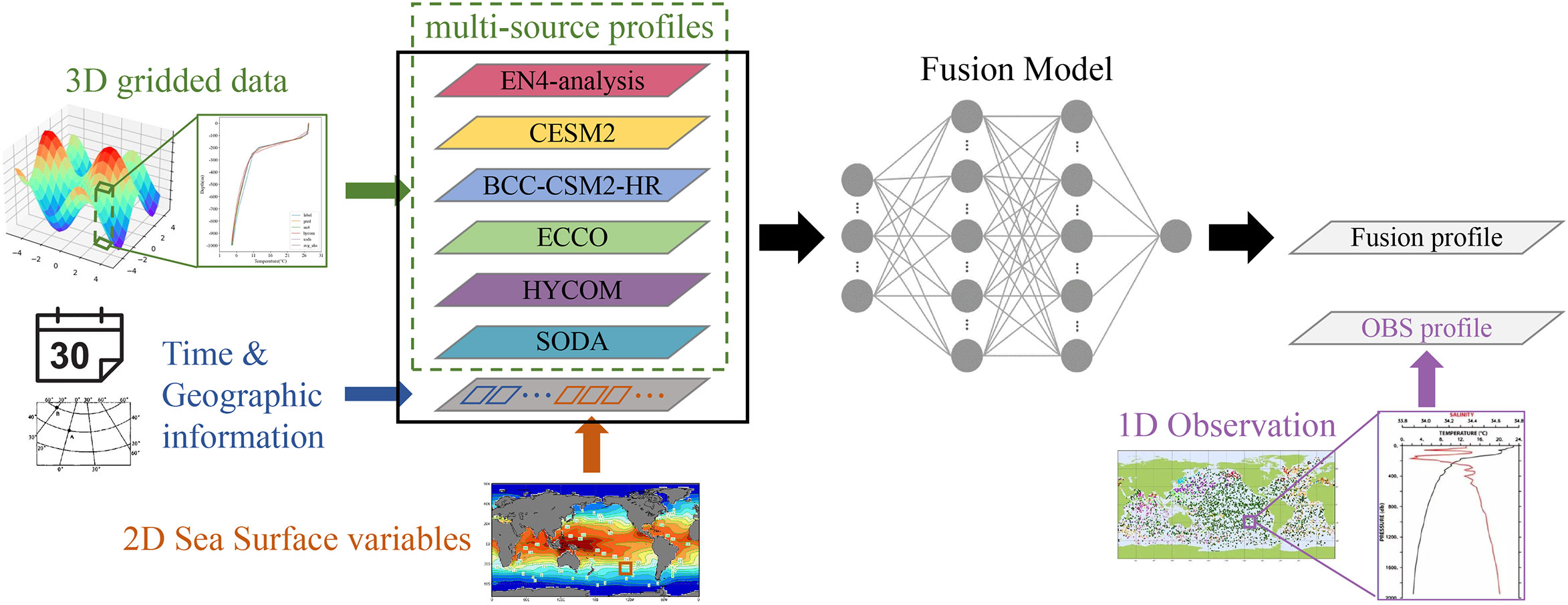
Figure 1 Framework for the intelligent fusion of multi-source heterogeneous ocean data.

In order to organize data from multiple sources into samples for model training, we produced samples based on the observation profiles collected in section 2.1, where one observation profile is equivalent to one sample. To better incorporate prior knowledge, such as the vertical structure of sea temperature, into the model and to suppress the spurious high-frequency signal of fusion data in the vertical direction, we chose to use the observation profile interpolated to standard layers as the label, as shown in Figure 1. Therefore, a label has a dimension of 1×D, where D is the number of vertical standard levels (23 in this work). The deepest effective sea temperatures were used to fill the missing data produced by seafloor terrain, and the filled data were not taken into account in the loss function. We reserved 10% of all samples as the test set for validation of model performance.

The dimension of sample features is C×D, where C=M+1 is the number of channels in the input layer of the fusion model, M is the number of 3D gridded datasets, and M=6 in the current study. As shown in Figure 1, the first six channels are vertical profiles of EN4-analysis, HYCOM, SODA, ECCO, CESM2, and BCC-CSM2-HR that correspond to the sample label in the temporal and spatial dimensions. The last channel provides the spatial data (latitude and longitude), the temporal data (year and month), and the sea surface data (ERSST, OISST, HadiSST, AVSIO SLA, and CCMP) corresponding to the sample label, with the remaining locations filled with zeros.

3.1 Model structures of the ODF-Net

The ODF-Net, shown in Figure 2A, is a variant of the 1D-ResNet model. There are three distinct sections to this design. To accomplish the task of extracting shallow features from multi-source ocean data, block A contains a 1D convolutional layer that uses a 3×1 kernel in addition to two GAMs. Blocks B and C, depicted in Figures 2B, C, respectively, are composed mostly of 1D convolutional layers with a 3×1 kernel, dropout layers (dropout probabilities of 0.5), and skip-connection structures to harvest the deep features. Block D is a decoding block that fully integrates sea temperature data from many sources through the use of a combination of shallow and deep features.

FIGURE 2

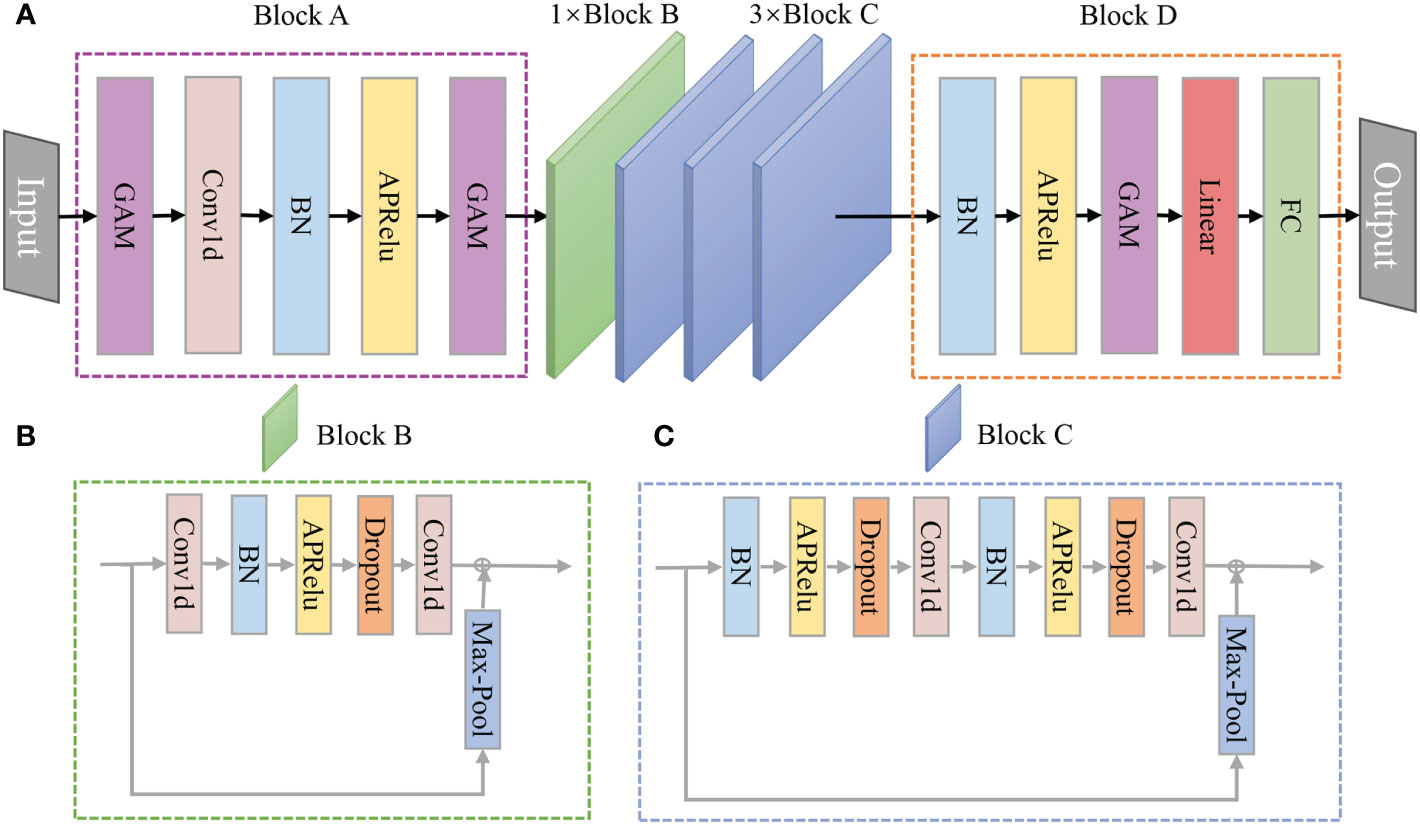
Figure 2 Structures of (A) the ODF-Net, (B) Block B, and (C) Block C.

In the ODF-Net, we choose to use the more advanced Adaptively Parametric Rectifier Linear Unit (APReLU) activation function rather than the more common ReLU activation function used in the 1D-ResNet. When the original features are less than zero, APReLU runs each sample through a small fully connected network to produce matching weights, which are then used as coefficients of the original features to provide a more flexible method of nonlinear transformation (Zhao et al., 2020).

3.2 GAMs in the ODF-Net

Improving the model’s interpretability assists with both understanding the deep learning model’s complex decision-making foundation and guaranteeing the model’s reliability (Xu et al., 2021). Giving neural networks an attention mechanism improves their ability to learn by focusing on the relevant important feature while discarding the rest. In order to emphasize the interaction of multiple sources of information at different depth levels and to enable the model to capture important features in both dimensions, we modify the GAM (Liu et al., 2021) and redesign the sub-modules. Figure 3A depicts the GAM’s overall attention mechanism process, which sequentially combines channel attention and spatial attention. Given input features F₁ the intermediate state F₂ and output F₃ are defined as

FIGURE 3

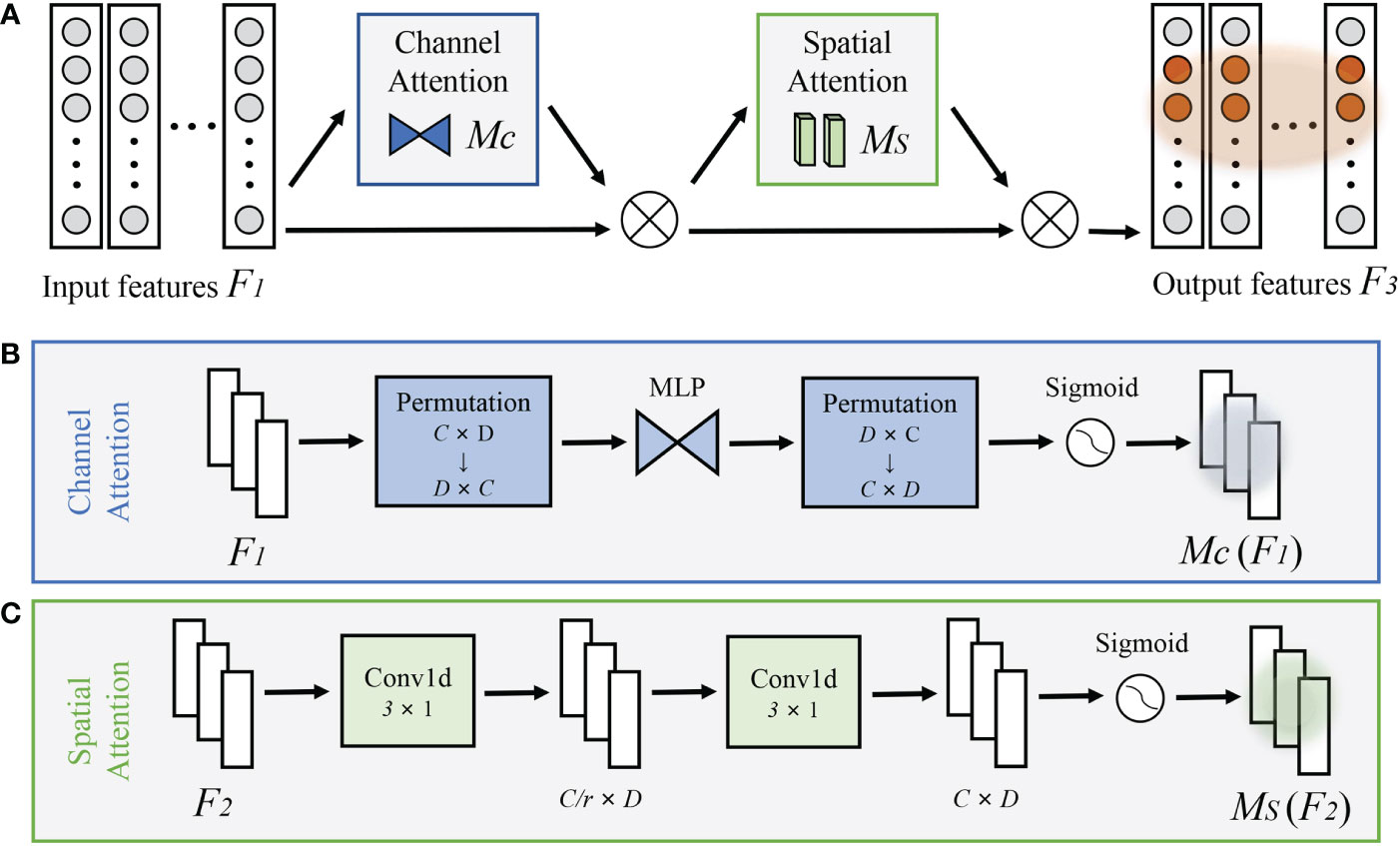
Figure 3 (A) The overview of redesigned GAM. The structures of (B) channel attention submodule, and (C) spatial attention submodule.

$\begin{array}{ll}{F}_2=M_C(F_1)\otimes F_1& (3)\end{array}$

$\begin{array}{ll}{F}_3=M_S(F_2)\otimes F_2& (4)\end{array}$

where M_c and M_s are the channel attention and spatial attention weights, respectively, indicating the model’s degree of attention to distinct channels and depth levels of input features. ⊗ denotes the multiplication operation by element. For the first GAM, in particular, channel attention reflects the importance of different sources, while spatial attention reflects the model’s concentration on diverse physical depth levels.

A major part of the channel attention submodule is shown in Figure 3B. When extracting information in two dimensions, 2D permutation is employed, and then a two-layer neuron network is used to magnify the dependence between channels and depth levels across dimensions. Each channel’s weights are then calculated using the sigmoid function. Figure 3C depicts the spatial attention submodule, which uses two convolutional layers to aggregate information from different depths and a sigmoid function to determine the weights of each depth.

3.3 Design of loss function

In order to integrate prior knowledge such as the vertical structure of sea temperature into the model and reduce the spurious high-frequency signal of fusion data in the vertical direction, the vertical gradient and integral of the sea temperature profile were added to the loss function, which is calculated as

$\begin{array}{ll}Los{s}_1=RMSE+\alpha ·Los{s}_{ST\_Grad}+\beta ·Los{s}_{Cumsum}& (5)\end{array}$

where Loss_{ST_Grad} is the sea temperature gradient constraint, Loss_Cumsum is the sea temperature profile integral constraint. α and β are hyperparameters, which were determined as 0.004 and 0.02 respectively through comparison experiments. The Loss_{ST_Grad} and Loss_Cumsum are defined as

$\begin{array}{ll}Los{s}_{ST\_Grad}=\sqrt{\frac{1}{N}\sum _{i=1}^N{(ST\_Gra{d}_{label, i}-ST\_Gra{d}_{pred, i})}^2},ST\_Gra{d}_k=\frac{T_{k+1}-T_k}{Z_{k+1}-Z_k}& (6)\end{array}$

$\begin{array}{ll}Los{s}_{Cumsum}=\sqrt{\frac{1}{N}\sum _{i=1}^N{(Cumsu{m}_{label, i}-Cumsu{m}_{pred, i})}^2},Cumsum={\sum }_{k=1}^M{T}_k& (7)\end{array}$

where ST_Grad and Cumsum represent the vertical gradient and the vertical integral of the sea temperature profile, respectively. T_i denotes the sea temperature value of the i-th level and Z_i denotes the vertical depth of the i-th level.

Meanwhile, to determine whether the loss function with gradient and integral constraints may improve the model’s fusion performance, a comparative experiment was run with the loss function Loss₂=RMSE, and the experimental results are provided in Table 1. R² is the coefficient of determination, a value ranging from 0 to 1 that indicates how effectively a statistical model predicts an outcome. The closer a model’s R² is to 1, the better it is at making predictions. Equation 8 gives the calculation of R².

TABLE 1

Table 1 Comparison of metrics on test set using different loss functions.

$\begin{array}{ll}{R}^2=\frac{{\sum }_{i=1}^N{(f_i-\overline{y})}^2}{{\sum }_{i=1}^N{(y_i-\overline{y})}^2}& (8)\end{array}$

where f_i and y_i represent the i-th prediction and label, respectively. $\overline{y}$ denotes the averaged value of all labels. The model with Loss₁ has nearly the same root mean square error (RMSE) as the model with Loss₂ but the sea temperature profile gradient error (STPGE) is reduced by 4%, indicating that the addition of physics-based prior knowledge constraints in the loss function has an enhancement effect on the vertical structure of the fusion sea temperature.

3.4 Ablation studies

Four sets of experiments (Exp0–Exp3) were designed to validate the favorable impacts of GAM and APReLU on the fusion model. Exp0 is the baseline, which does not include GAM or APReLU. Exp1 includes GAM, and Exp2 includes APReLU. Exp3 includes both GAM and APReLU, i.e., the ODF-Net. In addition, we designed Exp4 to do the same fusion task using Transformer (Vaswani et al., 2017), a state-of-the-art model for sequence-to-sequence learning, in order to validate the ODF-Net’s performance in comparison to other models. The transformer’s hyperparameters were tuned, and the encode dimension, number of attention heads, number of identical layers, query vector length, and key vector length were all set to 128, 8, 6, 16, and 16, respectively.

Table 2 shows a comparison of test results from the five sets of experiments. Comparing Exp1 and Exp0, GAM reduces RMSE by 2.87% and STPGE by 4.28%; comparing Exp2 and Exp0, APReLU reduces RMSE by 4.33% and STPGE by 5.32%; comparing Exp3 and Exp0, GAM and APReLU reduce RMSE by 6.98% and STPGE by 6.86%. As a result, GAM and APReLU considerably increase model performance. The comparison of Exp4 and Exp3 shows that the ODF-Net outperforms the Transformer in all metrics, including RMSE, STPGE, and R². The quantities of trainable parameters are listed in the third column of Table 2 with M representing 10⁶, the higher the value, the more complicated the model. The amount of trainable parameters in the ODF-Net is only about 60% of the Transformer, demonstrating that the ODF-Net we developed is lightweight and high-performance.

TABLE 2

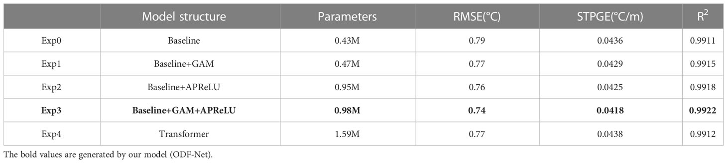
Table 2 Comparison of metrics on test set using different model structures.

4 Results and discussion

This section begins with an evaluation of the ODF-Net’s performance using in situ observations from the reserved test set. The model’s interpretability was then examined by collecting the attention weights of the first GAM in the ODF-Net. Finally, the global sea temperature dataset developed by the ODF-Net was examined to verify the method’s practicality.

4.1 Performance of the ODF-Net

To verify the accuracy of the fusion model, we compared the RMSE, STPGE, and R² of all eight data sources, including ODF-Net predictions, six sets of fused data, and their ensemble average data (EAD), with in situ observations. Table 3 summarizes the accuracy of different datasets over the test set using the metrics mentioned above. As Table 3 suggests, ODF-Net predictions are optimal on all evaluation metrics. ODF-Net predictions have an average RMSE of 0.74°C, while other data sources have RMSEs greater than 0.9°C. ODF-Net predictions have an average STPGE of 0.042°C/m, while other data sources have average STPGEs greater than 0.046°C/m. The ODF-Net improves both the accuracy and the vertical structure of the fusion sea temperature.

TABLE 3

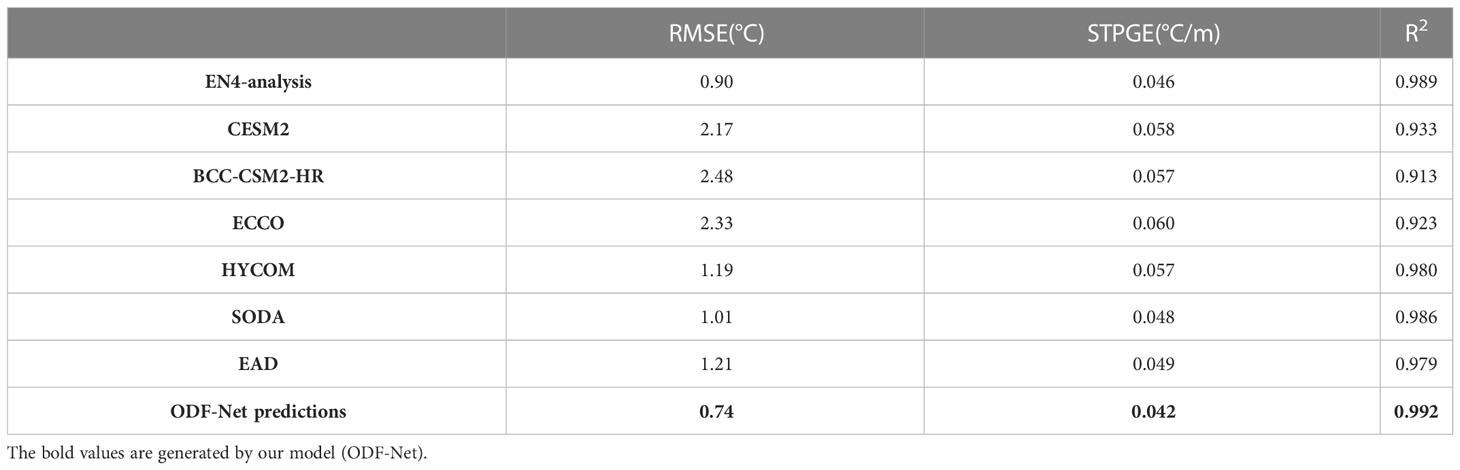
Table 3 Comparison of metrics on test set of different data sources.

The spatial distribution of RMSE is depicted in Figures 4A, B. ODF-Net predictions are more accurate than EAD’s in almost all regions, especially in areas with large gradients such as the Gulf Stream, the Kuroshio Extension, and the West Wind Drift, where the improvement is noticeable. Figure 4C shows the spatial distribution of the percentage improvement in R² of ODF-Net predictions with observation profiles versus R² of EAD predictions with observation profiles. Statistical examination of the test set reveals that R² of ODF-Net predictions is greater than EAD for 78.51% of the profiles. The improvement is more significant in areas with large gradients, such as the boundary current regions, which are similar to the spatial distribution of RMSE, suggesting that the deep learning model learns more correct information from multiple datasets.

FIGURE 4

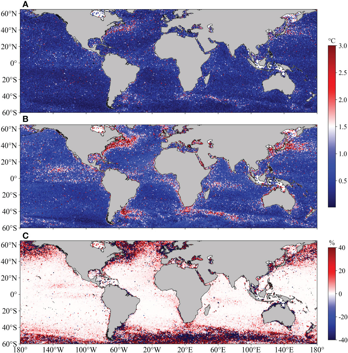
Figure 4 Spatial distribution of RMSE between (A) the ODF-Net, (B) EAD and EN4-profiles observations; (C) Spatial distribution of increase percentage in R² of the ODF-Net relative to EAD.

The distribution and variation of sea temperatures in different ocean areas and depth levels exhibit distinct characteristics due to the effects of several factors, such as solar radiation, land-sea distribution, ocean currents, and monsoons (Chen et al., 2002; Li et al., 2020). To examine the fusion effect, we evaluated the accuracy of ODF-Net predictions at different depth levels by region. The global ocean was divided into five oceans, which are the Pacific Ocean, the Atlantic Ocean, the Indian Ocean, the Arctic Ocean, and the Southern Ocean. ODF-Net performance in the five oceans and global regions is then discussed.

Here, we examined the time average RMSEs of eight data sources at different depth levels in the five oceans and global regions, including CESM2 (green line), BCC-CSM2-HR (red line), ECCO (purple line), SODA (pink line), EN4-analysis (orange line), HYCOM (brown line), EAD (gray line), and ODF-Net predictions (blue line) (Figure 5). The time average RMSEs in the vertical direction of eight data sources varied in each of the five oceans, but the RMSE of ODF-Net predictions at different depth levels is significantly lower than that of other data sets in each ocean as well as the global region. This indicates that the proposed ODF-Net performs better on a global scale. The accuracy improvement in ODF-Net predictions above the thermocline is greater than in other deeper layers, particularly at the thermocline with the largest vertical gradient. This might be attributed to the large number of thermocline observations, which enables the ODF-Net to learn the bias between other data sources and observations.

FIGURE 5

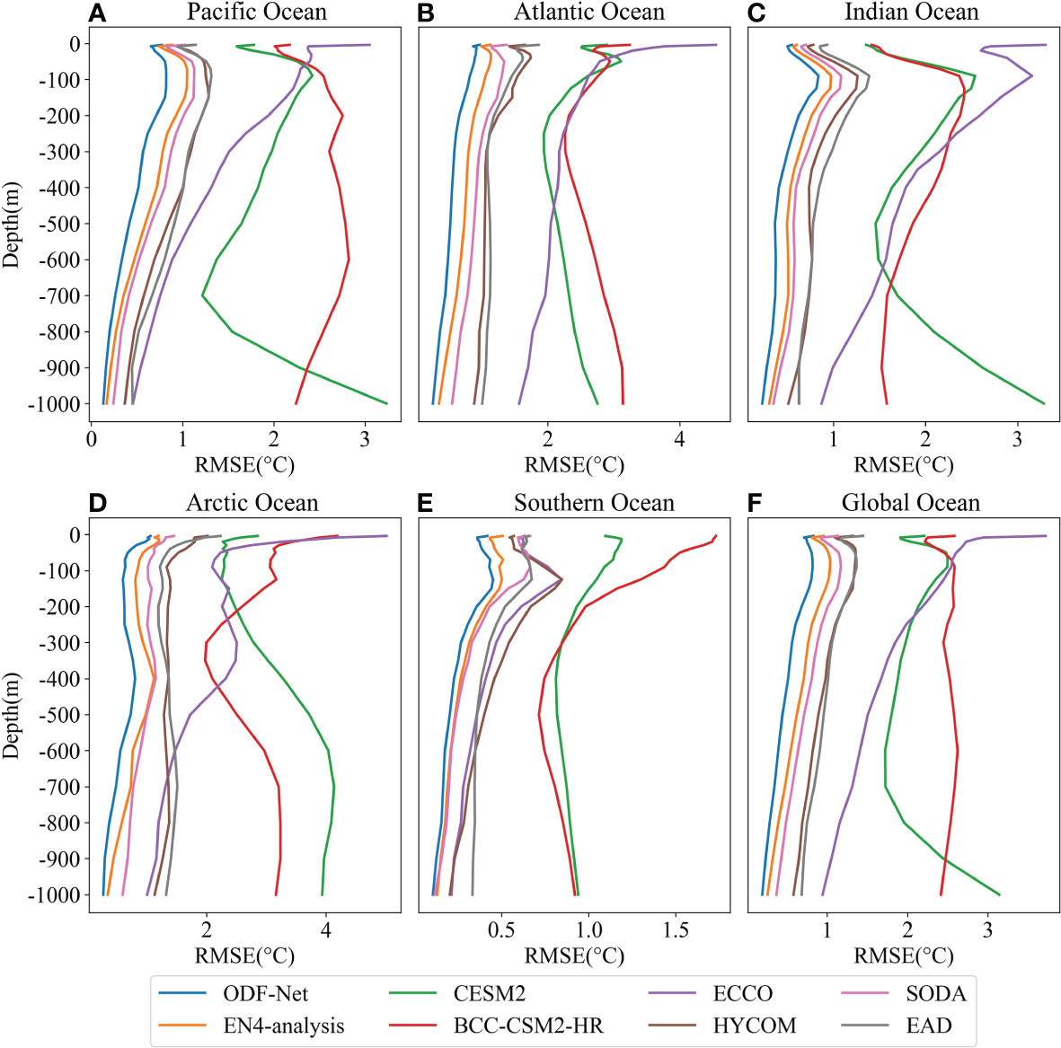
Figure 5 Vertical distribution of time-averaged RMSEs in (A) Pacific Ocean, (B) Atlantic Ocean, (C) Indian Ocean, (D) Arctic Ocean, (E) Southern Ocean, and (F) Global Ocean.

The Taylor diagram incorporates numerous assessment measures that are commonly used to evaluate model performance, including the correlation coefficient (COEF), root mean square error (RMSE), and standard deviation (STD) (Taylor, 2001). Taylor diagrams were utilized to more thoroughly and objectively analyze the statistical connections between various data points and observations in this work. Taylor diagrams of sea temperatures in the five oceans and global regions based on nine data sources, including projections (black dots) and observations (red dots) from ODF-Net are shown in Figure 6. Figure 6 shows that the results from several datasets vary widely, while the predictions generated by ODF-Net consistently and comprehensively outperform those generated by any other dataset. ODF-Net predictions are unbiased with a high level of correlation. The ODF-Net also has different outcomes depending on location. The performance of the ODF-Net in the Pacific, Atlantic, and Indian Oceans was comparable to that of the global region (Figures 6A–C). Figures 6D, E illustrate that the performance of the ODF-Net model in the Northern and Southern Oceans still needs to be improved. The main reason is that the performance of ODF-Net is highly dependent on high-quality observations, which are much less available in the Arctic and Southern Oceans than in other regions.

FIGURE 6

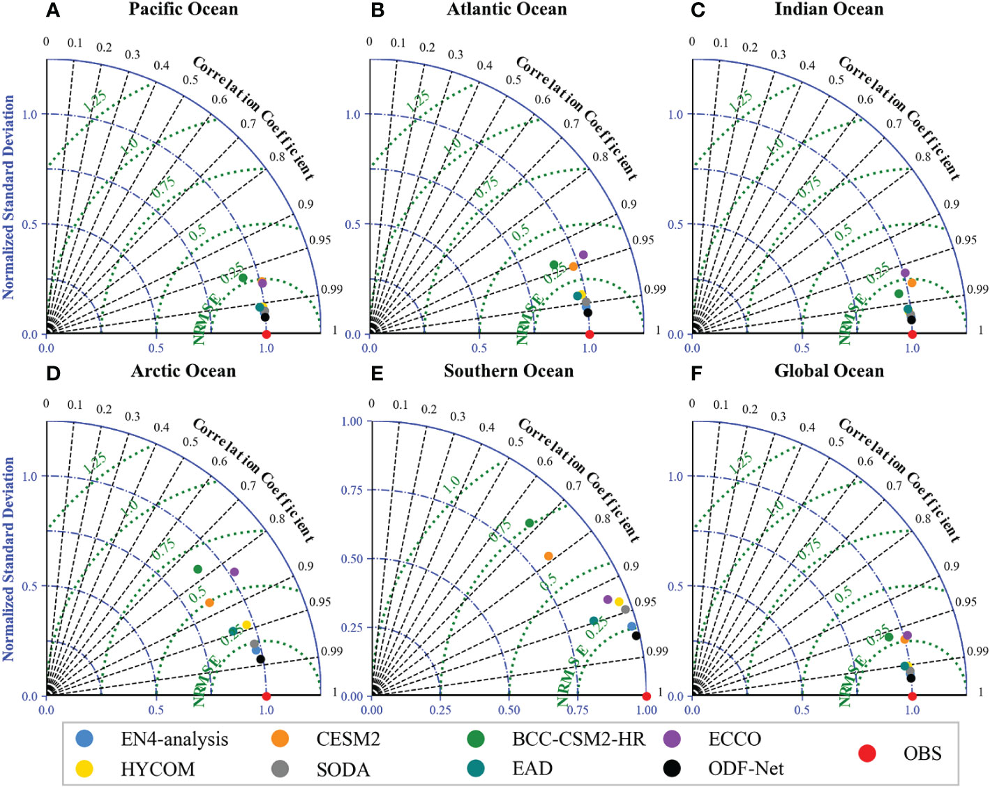
Figure 6 Time-averaged Taylor diagram in (A) Pacific Ocean, (B) Atlantic Ocean, (C) Indian Ocean, (D) Arctic Ocean, (E) Southern Ocean, and (F) Global Ocean.

4.2 Interpretability of the ODF-Net

Attention weights, as an intermediate output of the network model, can be used as a convenient tool to explain model decisions. Many studies have discussed the model interpretation ability of the attention weight distribution for neural network models based on attention mechanisms (Pruthi et al., 2019; Serrano and Smith, 2019; Wiegreffe and Pinter, 2019). In this study, we utilized attention weight distribution to analyze the contribution of multi-source ocean data as well as spatiotemporal information to the ODF-Net fusion process. Since multi-source data were sent directly to the first GAM in the ODF-Net, the attention weights could represent the contributions of the original ocean data as well as of the spatiotemporal information. We obtained the channel attention weight M_c and the spatial attention weight M_s of the first GAM, and since the GAM used a combination of channel and spatial attention serially, the global attention weight M_global is defined as:

$\begin{array}{ll}{M}_{global}=M_C\otimes M_S& (9)\end{array}$

Figure 7 shows a heat map of the global attention weight M_global. The top six rows illustrate the contribution of each of the 3D gridded datasets to the final fusion task, while each column represents the contribution of ocean data at various depth levels. As shown in Figure 7, the top three 3D gridded data contributors, in order, are EN4-analysis, SODA, and HYCOM, whereas ECCO, CESM2, and BCC-CMS2-HR contribute relatively little. The distribution of attention weights is rather reasonable, as the error between EN4-analysis and observed EN4-profiles is the smallest on the test set, followed by SODA and HYCOM, whereas the average errors are larger for ECCO, CESM2, and BCC-CMS2-HR. This implies that the ODF-Net has given more attention to high-precision data. In the spatial dimension, the attention weights of the shallow levels above 100 m are greater than those of the deeper levels below 100 m for EN4-analysis and SODA, the two datasets that received the most attention, and for other datasets, the weights of the deep levels are greater than those of the shallow levels. This is due to the fact that sea temperatures are more stable at deeper levels, and 3D gridded datasets at deeper levels are more accurate than those at shallow levels. Due to the extremely high correlation of sea temperature variations with latitude, latitude has the greatest weight in the last channel. In contrast, the attention weights of temporal information and sea surface data are not significantly different. The analysis of attention weights shows that the ODF-Net pays more attention to the data sources that are more accurate. At the same time, information from different depth levels of the same data source makes different contributions to the fusion process.

FIGURE 7

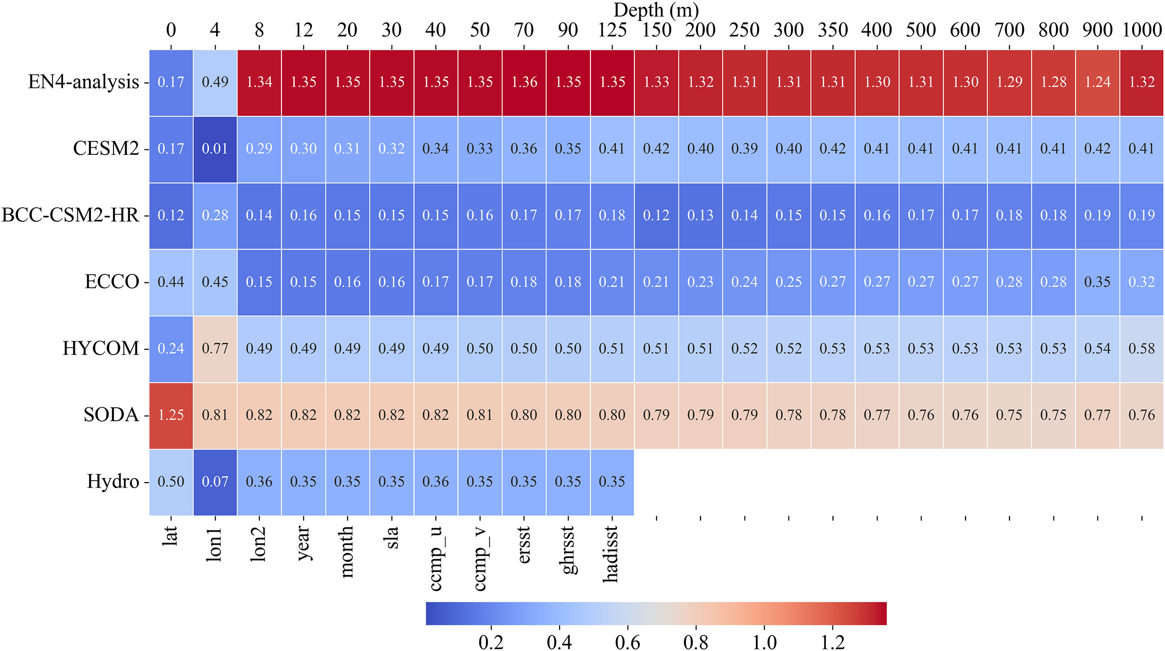
Figure 7 Heat map of GAM attention weights.

4.3 Evaluation of ODF-ST dataset

Since the purpose of this study is to accomplish accuracy, high resolution, and spatiotemporal continuous intelligent fusion of multi-dimensional, multi-source heterogeneous ocean data, we used the ODF-Net to generate a 3D sea temperature fusion dataset (ODF-ST dataset). ODF-ST dataset spans the years 1994 to 2017, with a spatial extent of the global ocean (180°W–180°E, 60°S–65°N), a monthly temporal resolution, and a spatial resolution of 0.25°. To assess the spatial rationality of the ODF-ST dataset, we compared the fusion SST with that of OISST, the spatial distribution of fusion sea temperature profiles, and sea temperatures at different levels with WOA18 (Boyer et al., 2018). To assess the temporal rationality of the ODF-ST dataset, we compared the fusion sea temperature profiles with Tropical Atmosphere Ocean Array (TAO) monthly observation profiles. Finally, we evaluated the ENSO index time series calculated with fusion sea temperature.

The global climatic SSTs (averaged from 1994 to 2017) of the ODF-ST dataset and the OISST are shown in Figure 8, where both SSTs have a “low-high-low” distribution from north to south, with a notable high-value area in the mid-western Pacific Ocean and a center SST of nearly 29°C. The transition of 25°C isotherms in the east-central Pacific Ocean (red frame area) is similar. The differences in SSTs are in the range of 0.5°C in most regions, indicating that the distribution of ODF-ST SST is acceptable and trustworthy. ODF-ST SST is significantly higher than OISST in Hudson Bay, the Mediterranean Sea, the southwestern coast of Africa, and the western Okhotsk Sea, but markedly lower than OISST in the northwestern and southwestern Atlantic Ocean and the southeastern Okhotsk Sea, possibly due to more complex changes in nearshore currents and sparse observations.

FIGURE 8

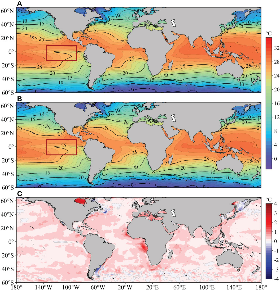
Figure 8 Global climatic (1994~2017) SST distribution of (A) ODF-ST dataset, (B) OISST, and (C) their difference.

The distribution of global climatic sea temperatures (averaged from 1995 to 2017) between the ODF-ST dataset and WOA18 at 500 m (Figures 9A–C) and 900 m (Figures 9D–F) shows that the ODF-ST sea temperature is very similar to WOA18. From north to south, both 500 m sea temperatures exhibit a “low-high-low-high-low” distribution, with noticeable high-value areas in the northwest Atlantic Ocean, the Mediterranean Sea, the southwest Indian Ocean, and the northwest Pacific Ocean, with the center sea temperature of the high-value area in the northwest Atlantic Ocean being around 17°C. Both 900 m sea temperatures have obvious high-value areas in the mid-eastern Atlantic Ocean, the Mediterranean Sea, and the Gulf of Aden, with the center sea temperature of the high-value area in the Mediterranean Sea being around 15°C. The isotherm trends are also strikingly similar, with homologous transitions of 500 m sea temperatures in the northern Atlantic Ocean and the southern Indian Ocean(red frame area). The differences between 500 m and 900 m sea temperatures of the ODF-ST dataset and WOA18 in most regions are lower than 0.25°C. Differences in 500 m sea temperatures have noticeable positive and negative oscillations in the Gulf Stream, the Kuroshio Extension, the North Pacific Current, and the West Wind Drift. Differences in 900 m sea temperatures have noticeable positive and negative oscillations in the Nansha Islands and the West Wind Drift.

FIGURE 9

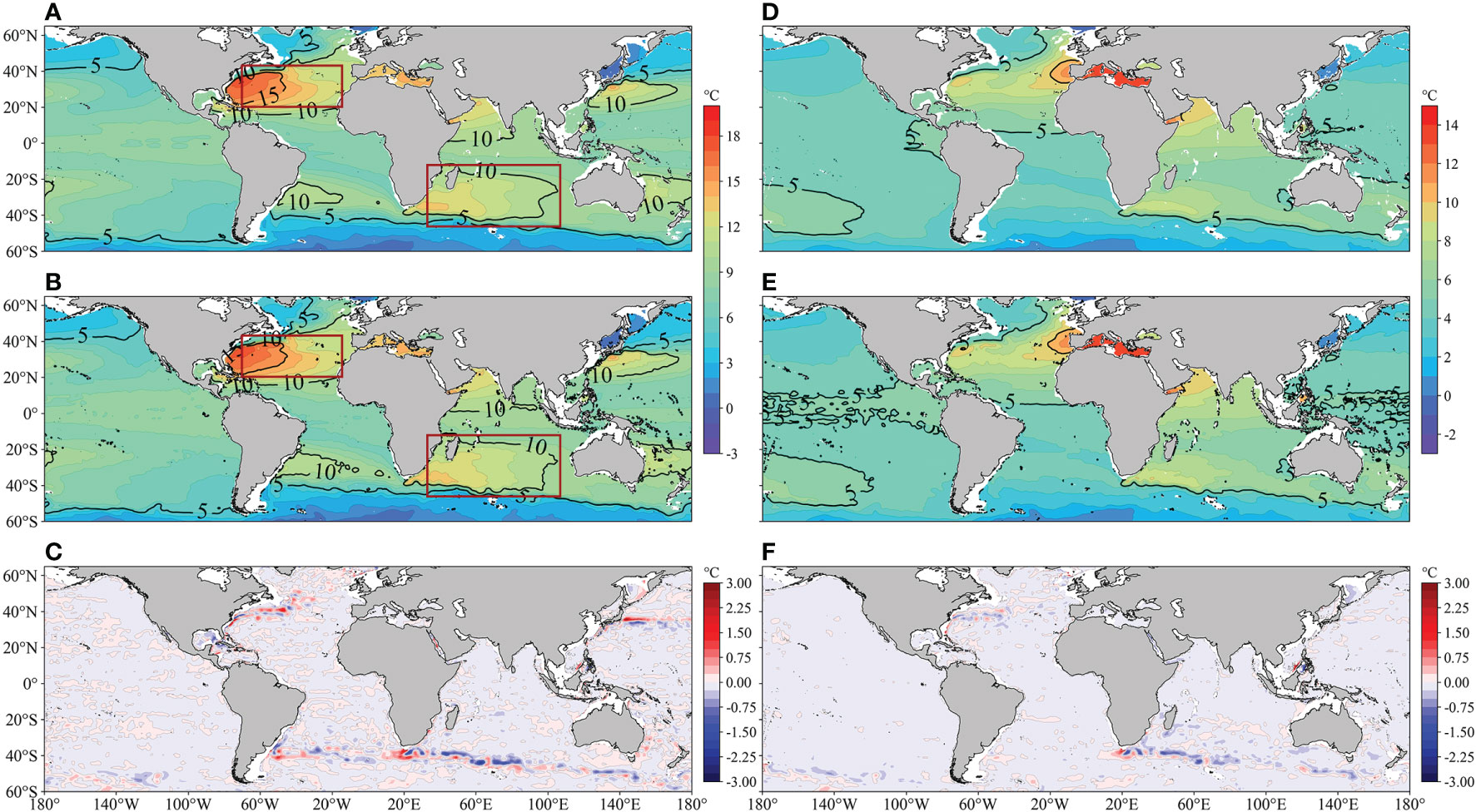
Figure 9 Global climatic (1995~2017) 500m sea temperature distribution of (A) ODF-ST dataset, (B) WOA18, and (C) their difference; Global climatic (1995~2017) 900m sea temperature distribution of (D) ODF-ST dataset, (E) WOA18, and (F) their difference.

To evaluate the rationality of ODF-ST sea temperature in the vertical direction, we averaged sea temperatures from the ODF-ST dataset and WOA18 in the longitudinal and latitudinal directions and then compared their sea temperature profiles along the latitudinal (Figures 10A–C) and longitudinal (Figures 10D–F) directions. The profile along the latitudinal direction demonstrates that the ODF-ST dataset and WOA18 both have a high sea temperature value of 28°C in-depth levels over 100m near 5°N. The isotherms exhibit evident grooves in the northern and southern hemispheres’ mid-latitudes. The difference in sea temperature is mostly less than 0.25°C. ODF-ST sea temperature is about 0.5°C higher than WOA18 in depth over 80 m in the Northern Hemisphere.

FIGURE 10

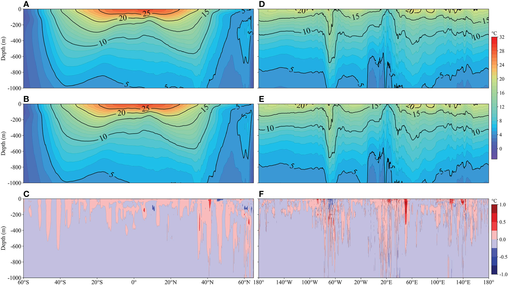
Figure 10 Longitudinal averaged climatic (1995~2017) sea temperature profiles along latitudinal direction of (A) ODF-ST dataset, (B) WOA18, (C) their difference and longitudinal direction of (D) ODF-ST dataset, (E) WOA18, and (F) their difference.

The profile along the longitudinal direction shows that the ODF-ST dataset’s isotherm change is essentially consistent with that of WOA18. Both have three regions with strong gradient variations located at 60°W–80°W, 0°–50°E, and 110°E–150°E, respectively. The differences in sea temperature are also higher in these regions, while differences in other regions are less than 0.25°C. The highly consistent ODF-ST sea temperature with WOA18 in the vertical direction implies that the spatial distribution of ODF-ST sea temperature is reasonable.

We used monthly TAO observation profiles from 1994 to 2017 to conduct a comparative analysis of temporal correlation in order to assess the temporal rationality of the ODF-ST sea temperature. Figure 11 depicts, for each observation site, the spatial distribution of the temporal correlation between the ODF-ST sea temperature and TAO observation profiles.The Pearson correlation coefficient has a range of 0.9755 to 0.9995 and a mean value of 0.996.Therefore, in the sea area where the TAO array is deployed, the temporal distribution of ODF-ST sea temperature is reasonable.

FIGURE 11

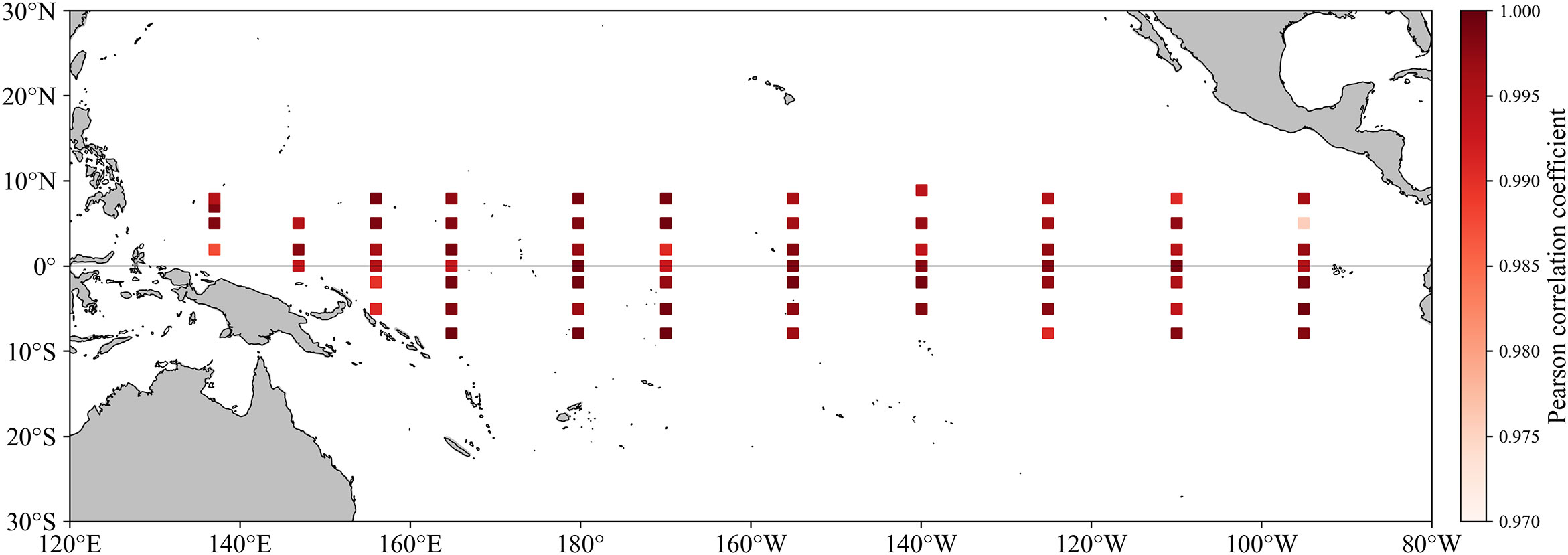
Figure 11 Spatial distribution of the temporal Pearson correlation coefficient between the ODF-ST sea temperature and TAO observation profiles.

To verify the ODF-ST dataset’s ability to capture the ENSO signal, Figure 12 illustrates the ENSO index time series in the Nino3.4 region (5°S–5°N, 170°W–120°W) of multiple sources from January 1994 to December 2017. Variations of the ENSO index in the ODF-ST dataset are generally consistent with those of ERSST and HadiSST and can reflect the significant El Niño years (1995, 1998, 2003, 2007, 2010, 2015) and La Niña years (1999, 2000, 2008, 2011, 2012, 2017).

FIGURE 12

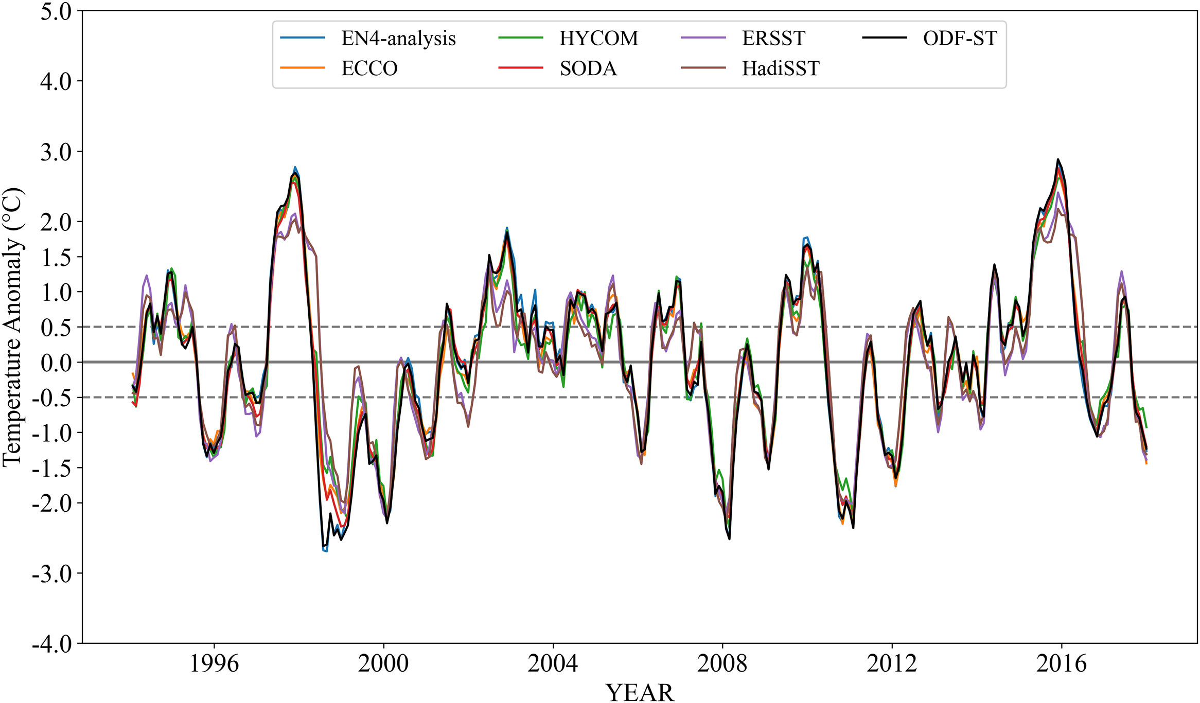
Figure 12 ENSO index time series in the Nino3.4 region of various sources.

We compared the Pearson correlation coefficient and RMSE of the anomalies in the Nino3.4 region of average sea temperatures above 100 m from different sources with the ENSO index provided by the U.S. Climate Prediction Center (NOAA/CPC) and discovered that the Pearson correlation coefficients of the ODF-ST dataset, HYCOM, ECCO, and SODA were all above 0.9 or higher, and the RMSEs of them were all below 0.5°C, indicating that the ODF-ST dataset’s sea temperature field could fairly reflect the ENSO signal.

5 Conclusion and future work

This paper presents an ODF-Net model for fusing ocean data from multiple sources, including 1D observation profiles, 2D sea surface datasets, and 3D gridded datasets. This approach is distinguished by its precision, speed, and interpretability. Instead of performing level-by-level, single-point ocean data assimilation, the vertical profile of the ocean is employed as the objective constraint. This enables us to incorporate physics-based previous knowledge and eliminate vertical high-frequency spurious signals. Global attention mechanisms are intended to guide ODF-net to crucial features from a diverse number of data sources and depth levels. The ODF-Net fusion sea temperature has a lower RMSE (0.74°C), a lower STPGE (0.042°C/m), and a higher R² than the fused data sources and EAD (0.99). A heat map of global attention weights was utilized to demonstrate the interpretability of the model. The ODF-Net assigned different weights to various characteristics of the datasets.

The most significant outcome of this study is a novel approach and paradigm for solving the age-old problem of integrating data from various, divergent ocean sources into a single whole. Nevertheless, the existing ODF-Net has only combined and investigated sea temperature; we will expand to include more factors of the marine environment. By adding new factors and examining their influence on the fusion outcomes, it is possible to further improve the fusion performance of the model. Moreover, the single-moment and single-profile data could be substituted with time-series ocean element fields in a realistic geographical region as fusion factors.

Data availability statement

The raw data supporting the conclusions of this article will be made available by the authors, without undue reservation.

Author contributions

MW and XH conceived and designed the research methodology. YX collected and pre-processed data. DW and MW conducted software, model validation and visualization. MW, DW and XH wrote and revised the manuscript. YL, RX, FX and JY gave important advice in the research and thesis writing process. All authors contributed to the article and approved the submitted version.

Funding

This work is supported by the National Key Research and Development Program of China (2021YFC3101600,2020YFA0607900, 2020YFA0608000) and the National Natural Science Foundation of China (42125503, 42075137).

Conflict of interest

Authors MW, DW and LY are employed by Ninecosmos Science and Technology Ltd.

The remaining authors declare that the research was conducted in the absence of any commercial or financial relationships that could be construed as a potential conflict of interest.

Publisher’s note

All claims expressed in this article are solely those of the authors and do not necessarily represent those of their affiliated organizations, or those of the publisher, the editors and the reviewers. Any product that may be evaluated in this article, or claim that may be made by its manufacturer, is not guaranteed or endorsed by the publisher.

References

Andersson T. R., Hosking J. S., Pérez-Ortiz M., Paige B., Elliott A., Russell C., et al. (2021). Seasonal Arctic sea ice forecasting with probabilistic deep learning. Nat. Commun. 12 (1), 1–12. doi: 10.1038/s41467-021-25257-4

PubMed Abstract | CrossRef Full Text | Google Scholar

Atlas R., Hoffman R. N., Ardizzone J., Leidner S. M., Jusem J. C., Smith D. K., et al. (2011). A cross-calibrated, multiplatform ocean surface wind velocity product for meteorological and oceanographic applications. B. Am. Meteorol. Soc 92 (2), 157–174. doi: 10.1175/2010BAMS2946.1

CrossRef Full Text | Google Scholar

Bauer P., Thorpe A., Brunet G. (2015). The quiet revolution of numerical weather prediction. Nature 525 (7567), 47–55. doi: 10.1038/nature14956

PubMed Abstract | CrossRef Full Text | Google Scholar

Bento P. M. R., Pombo J. A. N., Mendes R. P. G., Calado M. R. A., Mariano S. J. P. S. (2021). Ocean wave energy forecasting using optimised deep learning neural networks. Ocean Eng. 219, 108372. doi: 10.1016/j.oceaneng.2020.108372

CrossRef Full Text | Google Scholar

Boyer T. P., Baranova O. K., Coleman C., Garcia H. E., Grodsky A., Locarnini R. A., et al. (2018). World ocean atlas 2018. NOAA Atlas NESDIS 87, 1–207.

Google Scholar

Carton J. A., Chepurin G. A., Chen L. (2018). SODA3: A new ocean climate reanalysis. J. Climate 31 (17), 6967–6983. doi: 10.1175/JCLI-D-18-0149.1

CrossRef Full Text | Google Scholar

Carton J. A., Giese B. S. (2008). A reanalysis of ocean climate using simple ocean data assimilation (SODA). Mon. Weather Rev. 136 (8), 2999–3017. doi: 10.1175/2007MWR1978.1

CrossRef Full Text | Google Scholar

Chao Y., Li Z., Farrara J. D., Hung P. (2009). Blending sea surface temperatures from multiple satellites and in situ observations for coastal oceans. J. Atmos. Ocean. Tech. 26 (7), 1415–1426. doi: 10.1175/2009JTECHO592.1

CrossRef Full Text | Google Scholar

Chapman C., Charantonis A. A. (2017). Reconstruction of subsurface velocities from satellite observations using iterative self-organizing maps. IEEE Geosci. Remote S. 14 (5), 617–620. doi: 10.1109/LGRS.2017.2665603

CrossRef Full Text | Google Scholar

Chassignet E. P., Hurlburt H. E., Smedstad O. M., Halliwell G. R., Hogan P. J., Wallcraft A. J., et al. (2007). The HYCOM (hybrid coordinate ocean model) data assimilative system. J. Mar. Syst. 65 (1-4), 60–83. doi: 10.1016/j.jmarsys.2005.09.016

CrossRef Full Text | Google Scholar

Chelton D. B., Wentz F. J. (2005). Global microwave satellite observations of sea surface temperature for numerical weather prediction and climate research. B. Am. Meteorol. Soc 86 (8), 1097–1116. doi: 10.1175/BAMS-86-8-1097

CrossRef Full Text | Google Scholar

Chen G., Chapron B., Ezraty R., Vandemark D. (2002). A global view of swell and wind sea climate in the ocean by satellite altimeter and scatterometer. J. Atmos. Ocean. Tech. 19 (11), 1849–1859. doi: 10.1175/1520-0426(2002)019<1849:AGVOSA>2.0.CO;2

CrossRef Full Text | Google Scholar

Cheng L., Abraham J., Zhu J., Trenberth K. E., Fasullo J., Boyer T., et al. (2020). Record-setting ocean warmth continued in 2019. Adv. Atmos. Sci. 37, 137–142. doi: 10.1007/s00376-020-9283-7

CrossRef Full Text | Google Scholar

Chu X., He J., Song H., Qi Y., Sun Y., Bai W., et al. (2020). Multimodal deep learning for heterogeneous GNSS-r data fusion and ocean wind speed retrieval. IEEE J. STARS. 13, 5971–5981. doi: 10.1109/JSTARS.2020.3010879

CrossRef Full Text | Google Scholar

Courtier P., Thépaut J. N., Hollingsworth A. (1994). A strategy for operational implementation of 4D-var, using an incremental approach. Q. J. R. Meteor. Soc 120 (519), 1367–1387. doi: 10.1002/qj.49712051912

CrossRef Full Text | Google Scholar

Cressman G. P. (1959). An operational objective analysis system. Mon. Weather Rev. 87 (10), 367–374. doi: 10.1175/1520-0493(1959)087<0367:AOOAS>2.0.CO;2

CrossRef Full Text | Google Scholar

Danabasoglu G., Lamarque J. F., Bacmeister J., Bailey D. A., DuVivier A. K., Edwards J., et al. (2020). The community earth system model version 2 (CESM2). J. Adv. Model. Earth Sy. 12 (2), e2019MS001916. doi: 10.1029/2019MS001916

CrossRef Full Text | Google Scholar

Danard M. B., Holl M. M., Clark J. R. (1968). Fields by correlation assembly–a numerical analysis technique. Mon. Weather Rev. 96 (3), 141–149. doi: 10.1175/1520-0493(1968)096<0141:FBCAAN>2.0.CO;2

CrossRef Full Text | Google Scholar

Evensen G. (1994). Sequential data assimilation with a nonlinear quasi-geostrophic model using Monte Carlo methods to forecast error statistics. J. Geophys. Res. Oceans 99 (C5), 10143–10162. doi: 10.1029/94JC00572

CrossRef Full Text | Google Scholar

Forget G., Campin J. M., Heimbach P., Hill C. N., Ponte R. M., Wunsch C. (2015). ECCO version 4: An integrated framework for non-linear inverse modeling and global ocean state estimation. Geosci. Model. Dev. 8 (10), 3071–3104. doi: 10.5194/gmd-8-3071-2015

CrossRef Full Text | Google Scholar

Good S. A., Martin M. J., Rayner N. A. (2013). EN4: Quality controlled ocean temperature and salinity profiles and monthly objective analyses with uncertainty estimates. J. Geophys. Res. Oceans 118 (12), 6704–6716. doi: 10.1002/2013JC009067

CrossRef Full Text | Google Scholar

Ham Y. G., Kim J. H., Luo J. J. (2019). Deep learning for multi-year ENSO forecasts. Nature 573 (7775), 568–572. doi: 10.1038/s41586-019-1559-7

PubMed Abstract | CrossRef Full Text | Google Scholar

Hinton G. E., Salakhutdinov R. R. (2006). Reducing the dimensionality of data with neural networks. science 313 (5786), 504–507. doi: 10.1126/science.1127647

PubMed Abstract | CrossRef Full Text | Google Scholar

Huang B., Thorne P. W., Banzon V. F., Boyer T., Chepurin G., Lawrimore J. H., et al. (2017). Extended reconstructed sea surface temperature, version 5 (ERSSTv5): upgrades, validations, and intercomparisons. J. Climate 30 (20), 8179–8205. doi: 10.1175/JCLI-D-16-0836.1

CrossRef Full Text | Google Scholar

Jiao L., Zhao J. (2019). A survey on the new generation of deep learning in image processing. IEEE Access 7, 172231–172263. doi: 10.1109/ACCESS.2019.2956508

CrossRef Full Text | Google Scholar

Kahou S. E., Bouthillier X., Lamblin P., Gulcehre C., Michalski V., Konda K., et al. (2016). Emonets: Multimodal deep learning approaches for emotion recognition in video. J. Multimodal User In. 10 (2), 99–111. doi: 10.1007/s12193-015-0195-2

CrossRef Full Text | Google Scholar

Kopuklu O., Kose N., Rigoll G. (2018). Motion fused frames: Data level fusion strategy for hand gesture recognition. in. Proc. IEEE Conf. CVPR Workshops, 2103–2111. doi: 10.1109/CVPRW.2018.00284

CrossRef Full Text | Google Scholar

Kumar A., Wen C., Xue Y., Wang H. (2017). Sensitivity of subsurface ocean temperature variability to specification of surface observations in the context of ENSO. Mon. Weather Rev. 145 (4), 1437–1446. doi: 10.1175/MWR-D-16-0432.1

CrossRef Full Text | Google Scholar

Li Y. Y., Dong Q., Ren Y. Z., Kong F. P., Yin Z. (2020). Spatiotemporal characteristics of sea surface salinity of Indian and pacific oceans. J. Remote Sens. (Chinese) 24 (10), 1193–1205. doi: 10.11834/jrs.20209068

CrossRef Full Text | Google Scholar

Liu Y., Shao Z., Hoffmann N. (2021). Global attention mechanism: Retain information to enhance channel-spatial interactions. arXiv preprint arXiv. doi: 10.48550/arXiv.2112.05561

CrossRef Full Text | Google Scholar

Lorenc A. C. (1981). A global three-dimensional multivariate statistical interpolation scheme. Mon. Weather Rev. 109 (4), 701–721. doi: 10.1175/1520-0493(1981)109<0701:AGTDMS>2.0.CO;2

CrossRef Full Text | Google Scholar

Overpeck J. T., Meehl G. A., Bony S., Easterling D. R. (2011). Climate data challenges in the 21st century. science 331 (6018), 700–702. doi: 10.1126/science.1197869

PubMed Abstract | CrossRef Full Text | Google Scholar

Pruthi D., Gupta M., Dhingra B., Neubig G., Lipton Z. C. (2019). Learning to deceive with attention-based explanations. arXiv preprint arXiv. doi: 10.48550/arXiv.1909.07913

CrossRef Full Text | Google Scholar

Rayner N. A. A., Parker D. E., Horton E. B., Folland C. K., Alexander L. V., Rowell D. P., et al. (2003). Global analyses of sea surface temperature, sea ice, and night marine air temperature since the late nineteenth century. J. Geophys. Res. Atmos 108 (D14), 4407. doi: 10.1029/2002JD002670

CrossRef Full Text | Google Scholar

Reichstein M., Camps-Valls G., Stevens B., Jung M., Denzler J., Carvalhais N. (2019). Deep learning and process understanding for data-driven earth system science. Nature 566 (7743), 195–204. doi: 10.1038/s41586-019-0912-1

PubMed Abstract | CrossRef Full Text | Google Scholar

Reynolds R. W., Smith T. M., Liu C., Chelton D. B., Casey K. S., Schlax M. G. (2007). Daily high-resolution-blended analyses for sea surface temperature. J. Climate 20 (22), 5473–5496. doi: 10.1175/2007JCLI1824.1

CrossRef Full Text | Google Scholar

Salcedo-Sanz S., Ghamisi P., Piles M., Werner M., Cuadra L., Moreno-Martínez A., et al. (2020). Machine learning information fusion in earth observation: A comprehensive review of methods, applications and data sources. Inform. Fusion 63, 256–272. doi: 10.1016/j.inffus.2020.07.004

CrossRef Full Text | Google Scholar

Serrano S., Smith N. A. (2019). Is attention interpretable? arXiv preprint arXiv. doi: 10.48550/arXiv.1906.03731

CrossRef Full Text | Google Scholar

Stammer D., Balmaseda M., Heimbach P., Köhl A., Weaver A. (2016). Ocean data assimilation in support of climate applications: status and perspectives. Annu. Rev. Mar. Sci. 8, 491–518. doi: 10.1146/annurev-marine-122414-034113

CrossRef Full Text | Google Scholar

Strubell E., Ganesh A., McCallum A. (2019). Energy and policy considerations for deep learning in NLP. arXiv preprint arXiv. doi: 10.48550/arXiv.1906.02243

CrossRef Full Text | Google Scholar

Su H., Huang L., Li W., Yang X., Yan X. H. (2018). Retrieving ocean subsurface temperature using a satellite-based geographically weighted regression model. J. Geophys. Res. Oceans 123 (8), 5180–5193. doi: 10.1029/2018JC014246

CrossRef Full Text | Google Scholar

Su H., Wang A., Zhang T., Qin T., Du X., Yan X. H. (2021). Super-resolution of subsurface temperature field from remote sensing observations based on machine learning. Int. J. Appl. Earth Obs. 102, 102440. doi: 10.1016/j.jag.2021.102440

CrossRef Full Text | Google Scholar

Taylor K. E. (2001). Summarizing multiple aspects of model performance in a single diagram. J. Geophys. Res. Atmos 106 (D7), 7183–7192. doi: 10.1029/2000JD900719

CrossRef Full Text | Google Scholar

Thiébaux J., Rogers E., Wang W., Katz B. (2003). A new high-resolution blended real-time global sea surface temperature analysis. B. Am. Meteorol. Soc 84 (5), 645–656. doi: 10.1175/BAMS-84-5-645

CrossRef Full Text | Google Scholar

Vafaei B., Ezam M., Saghaei A., Bidokhti A. A. (2022). Automatic identification and tracking of meso-scale eddies in the Persian gulf using the pattern mining approach. Int. J. Environ. Sci. Technol. 19 (7), 6011–6022. doi: 10.1007/s13762-021-03779-0

CrossRef Full Text | Google Scholar

Vaswani A., Shazeer N., Parmar N., Uszkoreit J., Jones L., Gomez A. N., et al. (2017). Attention is all you need. NIPS 30, 5998–6008. doi: 10.48550/arXiv.1706.03762

CrossRef Full Text | Google Scholar

Wiegreffe S., Pinter Y. (2019). Attention is not not explanation. arXiv preprint arXiv. doi: 10.48550/arXiv.1908.04626

CrossRef Full Text | Google Scholar

Wu T., Yu R., Lu Y., Jie W., Fang Y., Zhang J., et al. (2021). BCC-CSM2-HR: a high-resolution version of the Beijing climate center climate system model. Geosci. Model. Dev. 14 (5), 2977–3006. doi: 10.5194/gmd-14-2977-2021

CrossRef Full Text | Google Scholar

Xiao C., Hu C., Chen N., Zhang X., Chen Z., Tong X. (2021). A genetic algorithm-assisted deep neural network model for merging microwave and infrared daily Sea surface temperature products. Front. Environ. Sci. 421. doi: 10.3389/fenvs.2021.748913

CrossRef Full Text | Google Scholar

Xu J., Yang J., Xiong X., Li H., Huang J., Ting K. C., et al. (2021). Towards interpreting multi-temporal deep learning models in crop mapping. Remote Sens. Environ. 264, 112599. doi: 10.1016/j.rse.2021.112599

CrossRef Full Text | Google Scholar

Yu D., Deng L. (2016). Automatic speech recognition Vol. 1 (Berlin: Springer).

Google Scholar

Zeng L., Levy G. (1995). Space and time aliasing structure in monthly mean polar-orbiting satellite data. J. Geophys. Res. Atmos. 100 (D3), 5133–5142. doi: 10.1029/94JD03252

CrossRef Full Text | Google Scholar

Zhang C., Wang D., Liu Z., Lu S., Sun C., Wei Y., et al. (2022). Global gridded argo dataset based on gradient-dependent optimal interpolation. J. Mar. Sci. Eng. 10 (5), 650. doi: 10.3390/jmse10050650

CrossRef Full Text | Google Scholar

Zhao M., Zhong S., Fu X., Tang B., Dong S., Pecht M. (2020). Deep residual networks with adaptively parametric rectifier linear units for fault diagnosis. IEEE T. Ind. Electron. 68 (3), 2587–2597. doi: 10.1109/TIE.2020.2972458

CrossRef Full Text | Google Scholar

Zhu Y., Bo Y., Zhang J., Wang Y. (2018). Fusion of multisensor SSTs based on the spatiotemporal hierarchical Bayesian model. J. Atmos. Ocean. Tech. 35 (1), 91–109. doi: 10.1175/JTECH-D-17-0116.1

CrossRef Full Text | Google Scholar