Environmental DNA in the Kuroshio reveals environment-dependent distribution of economically important small pelagic fish

1 Introduction

Fish production is critical for people’s livelihoods worldwide (Food and Agriculture Organization of the United Nations, 2020). Although aquaculture production has developed greatly, capture fishery production remains important, especially in marine fishery production where the percentage of capture contributed around 54% in 2016 (Food and Agriculture Organization of the United Nations, 2020). Small pelagic fish species, such as anchovy, sardine, and chub mackerel, have been major contributors to the total marine capture fishery production (Food and Agriculture Organization of the United Nations, 2020) especially in Japan, one of the most important fishery countries in the world (Ichinokawa et al., 2017). For example, the chub mackerel (Scomber japonicus) catch constituted around 2% of the world’s total catch in 2018 (Food and Agriculture Organization of the United Nations, 2020). Large-scale production of small pelagic fishes is based on prey zooplankton production. Small pelagic fishes also play critical roles in marine ecosystems as important prey of large predatory fishes, sea birds, as well as mammals, and connect lower and higher trophic levels (Cury et al., 2000; Duarte and Garcıía, 2004; Navarro et al., 2009; Cury et al., 2011; Navarro et al., 2017; Saraux et al., 2019). Thus, it is important to understand the distribution, migration, and response to climate variability of small pelagic fishes.

The resource (such as landings and body condition) of small pelagic fishes is influenced by many environmental factors, such as sea water temperature and chlorophyll-a concentration (Sumaila et al., 2011; Brosset et al., 2017; Quattrocchi and Maynou, 2017) as well as climate fluctuations or changes (Mantua et al., 1997; Brochier et al., 2013; Alheit et al., 2014; Pennino et al., 2020). For the Northwest Pacific area, rich in small pelagic fishes, the Kuroshio was found to influence climate, ecosystems, and fisheries (Yatsu et al., 2013). The Kuroshio is the western boundary current of the subtropical gyre in the North Pacific and a warm ocean current that flows from the northern Philippines and east of Taiwan, along the south coast of the Japanese Archipelago (Figure 1A). The section of the Kuroshio that flows eastward toward the open Pacific is called the Kuroshio Extension. The Kuroshio contains important spawning and nursery grounds, thought to be associated with many small pelagic fish species (Nakata et al., 2001; Sassa et al., 2006; Yatsu et al., 2013; Kaneko et al., 2018). Aggregation in the frontal eddies in the western boundary currents (Nakata et al., 2000; Okazaki et al., 2002; Mullaney and Suthers, 2013) as well as enhanced growth of small pelagic fish larvae in the frontal eddies (Okazaki et al, 2003) has been observed. Besides, the Kuroshio is thought to restrict the upstream movement of fishes on its inshore side (Kai and Motomura, 2022), which is hereinafter referred to as the “barrier effect”, these results indicate the importance of the frontal structure of the western boundary currents and their possible relationship to the distribution of small pelagic fishes.

FIGURE 1

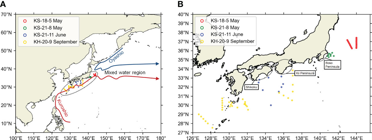
Figure 1 Location of the survey area of this study to the Northwest Pacific (A) and the zooming of the survey area (B). Maps were made in Spyder (Python 3.7) using Natural Earth data. Free vector and raster map data was obtained from @ naturalearthdata.com. The hollow circles represent the sampling stations. The stations from different cruises were distinguished by the colors of the hollow circles.

One of the possible effects of frontal structure on fish distribution is the thermal effect and oxygen demands (Pörtner and Knust, 2007). The relationship between environmental factors and the distribution of small pelagic fish in the ocean has been studied. Sabatés et al. (2006) found the distribution of round sardinella (Sardinella aurita) in the western Mediterranean was affected by the sea surface temperature (SST). Furthermore, Georgakarakos and Kitsiou (2008) analyzed the acoustic data of small pelagic fish and found SST and bathymetric depth are the environmental variables that provide the best spatial distribution model to predict the abundance. Similar studies have also been performed in the small-pelagic-fish-rich Northwest Pacific. Moreover, the winter catch per unit effort (CPUE) distribution of Japanese anchovy (Engraulis japonicus) in the Yellow and East China Seas demonstrated strong relationships with the salinity front and SST (Liu et al., 2020). The spatio-temporal variation of Japanese sardine (Sardinops melanostictus) population in the Sea of Japan was found to be influenced by SST, primary production, and ocean currents during 1970−1999 (Muko et al., 2018). Furthermore, Sassa et al. (2010) collected fish larvae in the southern East China Sea and discovered Scomber australasicus was distributed in the more southern and warmer (20 to 23°C versus 15 to 22°C) area than S. japonicus. Occurrence and density of Pacific saury Cololabis saira larvae and juveniles was found to be highly related to SST with an optimal temperature of 19–20°C (Takasuka et al., 2014). Therefore, these previous studies support an idea the SST is one of the main controlling factors which determine the distribution of small pelagic fish. This is not surprising because small pelagic fishes are ectothermic and have a small body size.

However, the SST dependency of small pelagic fish distribution is impacted by competition between fish species (Fuji et al., 2023). In the pelagic waters of the Northwest Pacific, the Pacific saury shifted to a cooler temperature range when the biomass of Japanese sardine expanded and the potential competition between the two species increased (Fuji et al., 2023). Small pelagic fish aggregate in the Kuroshio Front, and therefore, the competition between species might be enhanced and the effect of SST on distribution might be modified. This may especially be true for chub and blue mackerel, which are piscivorous fishes (Robert et al., 2010) whose main prey are anchovy (Nakatsuka et al., 2010; Robert et al., 2010). Currently there is no study showing a direct link between the distribution of chub and blue mackerel and that of Japanese anchovy. However, the distribution of Spanish mackerel, a predator of Japanese anchovy, highly depends on the distribution of Japanese anchovy (Liu et al., 2023). Consequently, in the aggregated frontal region, prey-predator interaction might alter the distribution characteristics of small pelagic fish.

Indeed, much is still unknown about the relationship between frontal structures, such as the Kuroshio Front, and small pelagic fish distribution. The frontal structures have complex and variable horizontal and vertical environmental conditions (Kasai et al., 2002; Nagai et al., 2012). Therefore, high horizontal and vertical resolution fish distribution data is needed to investigate the environmental effects and inter-specific effects on fish distribution in the frontal area. For larvae, it is possible to conduct high spatio-temporal resolution observations using small larval nets. However, for juveniles and adult fish, this is difficult because their swimming ability is high and large sampling nets are required. In addition, there is a limitation on obtaining information on vertical distribution differences of fish using fishing net sampling although there are multi-depth-sampling net systems. Acoustic sonar is another method for observing fish distribution but currently there are still problems with species identification (Wei et al., 2022). The local fishing catch data is usually needed as a reference in the species identification during acoustic sonar fish detection, which can be unfeasible if the fish species composition is expected to be complex (Georgakarakos and Kitsiou, 2008). Due to these limitations, it has been difficult until now to clarify the environmental and inter-specific effects on the distribution of small pelagic fish in the frontal structures.

The environmental DNA (eDNA) method is a novel technology used in organism surveys which has been developed in recent years. Organisms contain DNA that provides species identification information (Wolf et al., 1999; Ali et al., 2014). When DNA is released into the surrounding environment such as water, sediment, and soil (Thomsen and Willerslev, 2015; Barnes and Turner, 2016; Nevers et al., 2020) through feces, skin, scales, and other means (Poinar et al., 1998; Bunce et al., 2005; Lydolph et al., 2005), it is called eDNA. The sampling of fish eDNA is made possible by collecting and filtering water, enabling high-resolution observations of fish distribution in frontal regions. The procedure of collecting water can be simply performed and be combined with a conductivity temperature depth (CTD) system carried by a research vessel measuring the environmental factors at different depths (Yu et al., 2022). Therefore, the sampling of fish eDNA can be performed with a relatively high horizontal and vertical resolution together with the environmental measurements.

The eDNA method has been widely used for fish distribution surveys in inland and coastal waters worldwide (Minamoto et al., 2011; Kalchhauser and Burkhardt-Holm, 2016; Plough et al., 2018; Minegishi et al., 2019; Stat et al., 2019). Using eDNA analysis methods such as quantitative polymerase chain reaction (qPCR) and metabarcoding, information, including species and quantity, can be revealed. Recently, an optimized protocol for eDNA extraction in fish and robust qPCR conditions have been developed (Wong et al., 2020). A multiplex qPCR system was developed for the quantitative analysis of six small pelagic fishes’ eDNA (Wong et al., 2022): the Japanese sardine (hereafter sardine, S. melanostictus), Japanese anchovy (anchovy) E. japonicus, chub mackerel, blue mackerel (S. australasicus), Japanese jack mackerel (jack mackerel, Trachurus japonicus), and Pacific saury (saury, C. saira). The effectiveness of the multiplex qPCR system was confirmed by the detection of small pelagic fishes in the Kuroshio Extension (Yu et al., 2022). Here, as a new attempt, we used the validated multiplex qPCR system to analyze open ocean water samples from the Kuroshio Current system to explore the environment-dependent distribution patterns of several economically important small pelagic fishes. This study aimed to help improve the understanding of environmental and inter-specific effects on small pelagic fish distribution in the frontal region. The Kuroshio Current system was used as a testbed because it is one of the most productive areas of small pelagic fish. The improved understanding can be extended to other frontal regions including the Gulf Stream, as well as the Brazil, East Australian and the Agulhas Currents.

In this study, 488 sea water samples were collected during four Kuroshio cruises and used to detect the eDNA of six small pelagic fishes using qPCR. These fish species were chosen for their importance in fisheries. Subsequently, qPCR data were integrated with environmental data to estimate the influence of environmental parameters on the distribution of the target fishes. Among the six small pelagic fish we detected, the eDNA detection of saury and jack mackerel was very limited (details were shown in the Section 3.1), so the target fishes in this study were sardine, anchovy, chub mackerel, and blue mackerel.

Our study successfully revealed the environment-dependent spatial distribution characteristics of these target fishes in the Kuroshio Current system based on eDNA data. The success of this study supports the effectiveness of eDNA methods in revealing the relationship between fish and the environment. We expect a wider usage of its in other areas and on other species. In addition, we believe that our findings on the influence of predator–prey relationships will improve further studies and the understanding of small pelagic fish distribution patterns.

2 Materials and methods

2.1 Water sampling

Sea water samples were collected at 72 different stations during four cruises in the Kuroshio Current system (Figures 1, 2, Table S1). The research cruises KS-18-5 (May 2018), KS-21-8 (May 2021), and KS-21-11 (June 2021) were performed by the research vessel Shinsei-Maru, and the KH-20-9 (September–October 2020) research cruise was performed by the research vessel Hakuho-Maru. Shinsei-Maru and Hakuho-Maru are cooperative research vessels. Their cruise plan is based on open application systems (https://www.aori.u-tokyo.ac.jp/english/coop/index.html). The cruise period is limited to two weeks at the maximum for Shinsei-Maru. The cruise period of Hakuho-Maru is longer, but the open application is called every three years. Since it is not easy to conduct research cruises in a specific region for a sufficient period, we decided to cover the Kuroshio Current system by pooling data from different cruises.

FIGURE 2

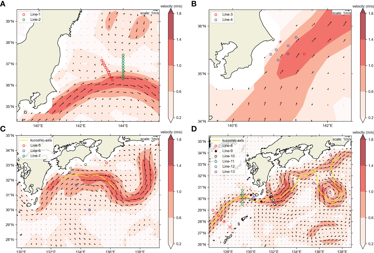
Figure 2 Positions of OceanDNA sampling stations in this study. Sampling area maps of (A) KS-18-5, (B) KS-21-8, (C) KS-21-11, (D) KH-20-9. Maps were made in Spyder (Python 3.7) using Natural Earth data. Free vector and raster map data was obtained from @ naturalearthdata.com. The hollow circles represent the sampling stations. Please note that the colors of hollow circles here were not used to distinguish the cruises. Colors of the background represent current speeds and arrows represent current velocity vectors on the sea surface (5-day mean of (A) May 10–14, 2018; (B) May 17–21, 2021; (C) June 17–21, 2021; (D) September 20–24, 2020) from Ocean Surface Current Analysis Real-time (OSCAR) data (ESR, 2009; https://podaac.jpl.nasa.gov/Data hosted and openly shared by the PO.DAAC, without restriction, in accordance with NASA’s Earth Science program Data and Information Policy). The position of Kuroshio axes was also estimated from OSCAR data, based on the method in Ambe et al. (2004).

Samples collected from three cruises, KS-18-5, KS-21-8, and KS-21-11, were pooled to analyze the effect of environmental factors (sea water temperature, temperature gradient, salinity, salinity gradient, dissolved oxygen concentration, chlorophyll-a concentration; see Section 2.5) on the small pelagic fishes in a wide area of the Kuroshio (Figures 1, 2). These cruises were all undertaken during the same season (May or June). Consequently, the effects of the seasonal environmental variability as well as seasonal distribution changes, such as seasonal migration of the target fishes, (Li et al., 2014; Sarr et al., 2021) was minimized. All four target species have long spawning periods lasting from winter to early summer, May–June overlapped with their spawning season. Furthermore, the target fishes in this study have wide spawning grounds in the southern coast of Japan (Hattori, 1964; Takasuka et al., 2008a; Nishikawa, 2018; Kanamori et al., 2021; Kume et al., 2021). Therefore, pooling samples from the three cruises are thought to be able to cover the distribution areas including the wide spawning grounds. The samples are expected to include the information from the mature stages and reproductive early life stages of the target fishes.

To further test the “barrier effect” of the Kuroshio, this study analyzed the differences in small pelagic fish distribution between the inshore and the offshore side of the Kuroshio using the samples of KS-21-11 and KH-20-9 because those cruises crossed the Kuroshio at the southern coast of Japan (the detailed method is shown in Section 2.7). Because these two cruises took place at different places and in different seasons, they were not pooled but analyzed separately.

The detailed water sampling methods of all cruises were as follows. In the KS-18-5 (19 stations, Figure 2A), water samples were collected from 13 depths (0, 5, 10, 15, 25, 30, 50, 80, 100, 125, 150, 200, and 300 m). In the KS-21-8 (eight stations, Figure 2B) and KS-21-11 (nine stations, Figure 2C), water samples were collected from seven depths (0, 10, 30, 50, 100, 150, and 200 m). At the KH-20-9 (32 stations, Figure 2D), water samples were collected at 10, 50, 100, and 150 m. Surface water samples (0 m depth) were collected using a clean bucket. Deeper water samples were collected using Niskin bottles combined with a CTD system that accurately determined the sampling depth and recorded environmental data. Sea water samples from each depth at each station were transferred to a clean plastic bag (Rontainer, Sekisui Chemical Co., Ltd., Tokyo, Japan) that had been rinsed three times with the sampled water. Each sample (~7 L in the KS-18-5 and ~10 L in the KS-21-8, KS-21-11, and KH-20-9) was weighed and then immediately filtered according to a previously described method (Yu et al., 2022). Sterivex-GP pressure filter units (0.22 μm pore size in the KS-18-5 and 0.45 μm pore size in the other cruises; Merck Millipore, Burlington, MA, USA) were used. Each filter unit has an inlet and an outlet (Wong et al., 2020). When the water filtration was finished, the interior of each filter unit was immediately filled with RNAlater (Thermo Fisher Scientific, Waltham, MA, USA) using a disposable syringe from the inlet and kept in a -30°C freezer before the next step to avoid DNA degradation. In addition to sea water samples, we also filtered negative controls on board (two 1.5 L Milli-Q water samples and two 10 L freshwater samples).

2.2 The eDNA extraction and purification

For the KS-18-5 samples, eDNA extraction and purification were performed by the Bioengineering Lab. Co., Ltd. (Kanagawa, Japan) using the procedure based on a previously described protocol (Miya et al., 2015), details of which have been previously described (Yu et al., 2022). For samples collected in the KS-21-8, KS-21-11, and KH-20-9, eDNA extraction and purification were performed using an in-house protocol described by Wong et al. (2020). Prior to extraction and purification, the equipment (silicon tubes, connectors, etc.) was treated with 1% bleach and rinsed with Milli-Q water to prevent contamination. Before each extraction, the Sterivex filter units were removed from the freezer and kept on ice to thaw the RNAlater which was then removed from the outlet by aspiration. A 2 mL lysis buffer mix (PBS 990 μL, Buffer AL 910 μL, Proteinase K 100 μL) was introduced through the outlet using a 2.5 mL syringe (Terumo Corporation, Tokyo, Japan). The outlet and inlet of each Sterivex filter unit were sealed, and all Sterivex filter units were incubated at 56°C for 30 min. After incubation, each Sterivex filter unit was centrifuged to collect the lysate, and the DNA in the lysate was extracted using the DNeasy Blood and Tissue Kit. For each column, we twice eluted the DNA with 75 μL of AE buffer to obtain a 150 μL DNA sample from each Sterivex filter unit.

2.3 The qPCR assays

Real-time qPCR assays were performed to measure the eDNA of six small pelagic fishes: sardine, anchovy, chub mackerel, blue mackerel, jack mackerel, and saury (Wong et al., 2022). Detailed sequence information for the primers and probes is listed in Table S2. In short, each multiplex real-time PCR reaction system (10 μL) included 1x Takara probe qPCR mix (Takara), 1x ROX reference Dye, 1 μg/μL BSA (A4161, Sigma-Aldrich), 0.8 μM forward and reverse primers for two species, 0.25 μM fluorescent probes for two species, and 2.5 µl of eDNA template. qPCR reactions were performed using an ABI 7900HT real-time PCR system (Thermo Fisher Scientific). The reactions entailed activation at 50°C for 2 min, denaturation at 95°C for 10 min, and then 50 cycles of denaturation at 95°C for 15 s and annealing and extension at 65°C for 1 min. All samples were assayed in duplicate.

We used qPCR assays to quantify the eDNA of the six small pelagic fishes in all sea water samples and negative controls (Wong et al., 2022). The plasmids of the six small pelagic fishes were used as the standard samples for the qPCR assays. Plasmids were diluted to a series of standard samples that contained 10¹–10⁷ copies of DNA molecules per 2.5 µl. During each qPCR assay, the Sequence Detection System Software v2.4.1 (SDS2.4) in the ABI 7900HT real-time PCR system recorded the Ct value in each eDNA sample (sea water sample or negative control) as well as the standard sample. The standard curve for each qPCR assay was determined using SDS 2.4, based on the Ct values and DNA copy numbers of standard samples. Then, the eDNA quantity (copy number per microliter) of each fish species in each eDNA sample was calculated using SDS 2.4, based on the Ct value in each eDNA sample and the standard curve. The quantity of eDNA was normalized against the volume of each filtered water sample. As shown in the Results (Section 3.1), no eDNA was detected from any negative control, therefore we assumed that there was no eDNA signal noise caused by contamination in this study. Consequently, when the eDNA quantity of one fish species in a sample was greater than 0, this species was judged to be present. In contrast, we used a normalized eDNA quantity (copy number per microliter) to represent the fish quantity at each sampling position (Takahara et al., 2012; Rourke et al., 2021; Everts et al., 2022). As the detection of saury and jack mackerel was very limited among our samples (Table S3), we chose sardine, anchovy, chub and blue mackerel as our target fishes for the following analyses.

2.4 Environmental data collection

Sea water temperature, salinity, dissolved oxygen concentration, and chlorophyll-a concentration were collected at every 1 m depth using a CTD system during sea water sampling (Table S4). Before the analysis, the chlorophyll-a concentration data were naturally log-transformed (as listed in Table S4, the lowest chlorophyll-a concentration value we recorded was 0.007 mg/m³ with no data for which the chlorophyll-a concentration value was zero).

The sea water temperature and salinity data were treated with a Gaussian filter (Gaussian sigma = 2.5, width = 11; performed by scipy.ndimage.gaussian_filter1d in Python 3.7) to eliminate instrument noise. Then, the temperature and salinity gradients were calculated from temperature data after Gaussian filtering (T) and salinity after Gaussian filtering (S) within a 10 m depth range. For example, the temperature and salinity gradients at a depth of 5 m were calculated as follows:

$$Temperature gradien{t}_{5 m}=(T_{10 m}-T_{0 m})/10 m$$

$$Salinity gradien{t}_{5 m}=(S_{10 m}-S_{0 m})/10 m$$

2.5 Generalized additive model

We used the Generalized additive model (GAM) to study the influence of environmental factors on the spatial distribution of the target fishes (presence/absence or quantity of eDNA). As explained in Section 2.1, for the GAM analyses in this study, data collected during the May–June cruises (KS-18-5, KS-21-8, and KS-21-11) were selected to prevent the effects of seasonal variability. At station D01 of the KS-21-11 cruise, the measurement of environmental factors failed because of sensor malfunction in the CTD. Thus, the D01 samples were not included in the analysis, and the data of the remaining 351 samples (from KS-18-5, KS-21-8, and KS-21-11) were included in the GAM analyses.

First, we used the GAM to investigate the influence of the six CTD-measured environmental factors (sea water temperature, temperature gradient, salinity, salinity gradient, dissolved oxygen concentration, and chlorophyll-a concentration) on the spatial distribution of the target fishes, which we referred to as the first GAM. Before the first GAM, we confirmed that collinearity did not occur among the six environmental factors using the Variance Inflation Factor method (VIF), calculated by the calculate_vif tool in Python 3.7. The depth (pressure) data were also measured by the CTD. However, many characteristics of sea water in the ocean, such as temperature, salinity, and dissolved oxygen concentration, change greatly with the depth (Webb, 2019). We also tested the collinearity when including depth in the environmental factors, and the results showed depth has the highest VIF value (~4.64) which suggested the collinearity between depth and other factors. Therefore, depth was not included in the list of environmental factors for GAM analysis.

Considering that mackerel (chub and blue) are piscivorous fishes (Robert et al., 2010) whose main prey are anchovy (Nakatsuka et al., 2010; Robert et al., 2010), we performed the second GAM to investigate their spatial distribution. Thus, the second GAM included anchovy and sardine quantities (both eDNA quantities) rather than the chlorophyll-a concentration as the food factor (i.e., the explanatory variable list included sea water temperature, salinity, temperature gradient, salinity gradient, dissolved oxygen concentration, and sardine and anchovy quantities). Using the VIF method, we also confirmed that collinearity did not occur among these environmental factors.

To perform the GAM analyses, we used pyGAM tools in Python 3.7 which use models to relate the predictor variables to the expected value of the dependent variable in the form shown below.

$$g(E[y|X])={\beta }_0+f_1(X_1)+f_2(X_2)+\dots +f_n(X_n)$$

$X.T = [X_1, X_2\mathrm{,...,}{X}_n]$ are the independent variables, y is the dependent variable, and g() is the link function that relates our predictor variables to the expected value of the dependent variable. The f_i() and feature functions were built using several penalized B-splines (six in this study). The pyGAM tools also judged the significance of each feature function, which suggested the significance of the effect of independent variables on dependent variable. In the first GAM, independent variables were sea water temperature (°C), salinity (PSU), temperature gradient (°C/m), salinity gradient (PSU/m), dissolved oxygen concentration (mL/L), and natural logarithmic transformed chlorophyll-a concentration (mg/m³). In the second GAM, independent variables were sea water temperature, salinity, temperature gradient, salinity gradient, dissolved oxygen concentration, and natural logarithmic transformed sardine and anchovy eDNA quantities. The predictor variable was the presence/absence or eDNA quantity of the target fishes. When examining the influence of environmental factors on the presence/absence of the four target fishes, we used PyGAM.LogisticGAM (n_splines = 6) in which the link function g() is a logit link and binomial error distribution was assumed. Therefore, the model was structured as follows.

$$log(\frac{P(y=1|X)}{P(y=0|X)})={\beta }_0+f_1(X_1)+f_2(X_2)+···+f_n(X_n)$$

When examining the influence of environmental factors on the eDNA quantity of the four target fishes, we used PyGAM.LinearGAM (n_splines = 6) in which the link function g() is an identity link, normal error distribution was assumed, and only samples where the target fish eDNA quantity was >0 were included. The model was structured as shown below.

$$E[y|X]={\beta }_0+f_1(X_1)+f_2(X_2)+···+f_n(X_n)$$

The fish eDNA quantity was logarithmically transformed before the GAM analyses. The GAM model with the lowest AICc (small-sample corrected Akaike Information Criterion) value was selected as the optimal model in the GAM analyses.

2.6 Temperature preference index analysis

The temperature preference index (TPI; Lluch-Belda et al., 1991) was used to evaluate how the spatial distribution of the target fishes (based on the presence/absence or eDNA quantity) actually varied among places with different sea water temperatures. If the effects of temperature are dominant, the TPI and temperature effects derived from the GAM are expected to show similar trends. To calculate the TPI, we divided the eDNA samples in this study into different temperature range groups (according to the CTD-measured temperature, groups were set every 2°C to ensure at least two samples per group). Then, for each target fish, the TPI of fish presence/absence (TPI_(0/1)) and fish eDNA quantity (TPI_(q)) in a specified temperature range was calculated as shown below.

$$TP{I}_{(0/1)}=\frac{N_1(T_{lower}~T_{upper})/{\sum }^{}{N}_1}{\left\{N_0(T_{lower}~T_{upper})+N_1(T_{lower}~T_{upper})\right\}/({\sum }^{}{N}_0+{\sum }^{}{N}_1)}$$

$$TP{I}_{(q)}=\frac{{\sum }_{T_{lower}}^{T_{upper}}{q}_{DNA}/{\sum }^{}{q}_{DNA}}{\left\{N_0(T_{lower}~T_{upper})+N_1(T_{lower}~T_{upper})\right\}/({\sum }^{}{N}_0+{\sum }^{}{N}_1)}$$

whereN₁ (N₀) means the number of samples with presence (absence) (of the given target species) within a temperature range between T_lower and T_upper. q_DNA means the DNA quantity (of the given target species). The numerator represents relative frequency of presence or DNA quantity within the specific temperature range and the denominator represents relative sampling effort. Therefore, a TPI >1 indicated the possibility that the target fish preferred that temperature range, while a TPI<1 indicated the opposite.

2.7 Analyses for the influence of the Kuroshio

The KS-21-11 and KH-20-9 cruises transected the Kuroshio Current (Figures 2C, D), and we investigated the influence of this current on the distribution of target fishes using samples collected from the above cruises. We compared the presence percentage of each target fish between samples collected on the offshore and inshore sides (the inshore side included the Kuroshio axis in this study). This axis represents the locally strongest part of the sea surface velocity field which was estimated based on the method introduced in Ambe et al. (2004). The percentage of samples present was calculated for either inshore side or offshore of KS-21-11 or KH-20-9, as well as for each station.

The percentage of samples at, for example, sardine on inshore side samples in the KS-21-11 cruise (R _{KS-21-11-IN-sardine}) was calculated as shown below.

$$R_{KS-21-11-IN-sardine}=\frac{ number of samples in which sardine presented}{ number of inshore side samples in KS-21-11 }*100\%$$

The percentage of samples at, for example, station A02 of the sardine (R_A02-sardine) was calculated as shown below.

$$R_{A02-sardine}=\frac{ number of samples in which sardine presented}{samples number in A02 station}*100\%$$

2.8 Ethics approval statement

This study did not involve any live animal experiments.

3 Results

3.1 qPCR assay results for six small pelagic fishes

Our qPCR assays did not detect any small pelagic fish eDNA in the negative controls (Milli-Q water and fresh water). Among the 488 sea water samples, chub mackerel eDNA was detected in 118 samples (24.18% of all samples), blue mackerel in 53 samples (10.86%), anchovy in 115 samples (23.57%), saury in 2 samples (0.41%), sardine in 184 samples (37.70%), and jack mackerel eDNA was detected in 15 water samples (3.07%). Detailed results of the qPCR assays are listed in Tables S3 and S5. As saury and jack mackerel showed limited distribution (<5%, Table S3), we excluded them from the analysis. The eDNA quantity vertical distributions of each species are shown in Figures 3 and S1–S9. DNA from the four target fishes was detected from water samples taken at various depths (Figures 3, 4) and horizontal locations (Figures 5, S10–13), but samples containing high eDNA quantities were mostly located above 50 m depth (Figure 4). As for the horizontal distribution in different depth layers, the eDNA of all target fishes were more abundant in the ocean area around the Boso Peninsula, especially in the water layer above 50 m depth (Figures S10, 11). A large number of chub mackerel eDNA was also located close to the Kii Peninsula and Shikoku (Figures S10–13). Generally, the eDNA of target fishes are more common in the inshore (northern) side than the offshore (southern) side of the Kuroshio axis (the Kuroshio Extension) (Figures S3–S9 and 3).

FIGURE 3

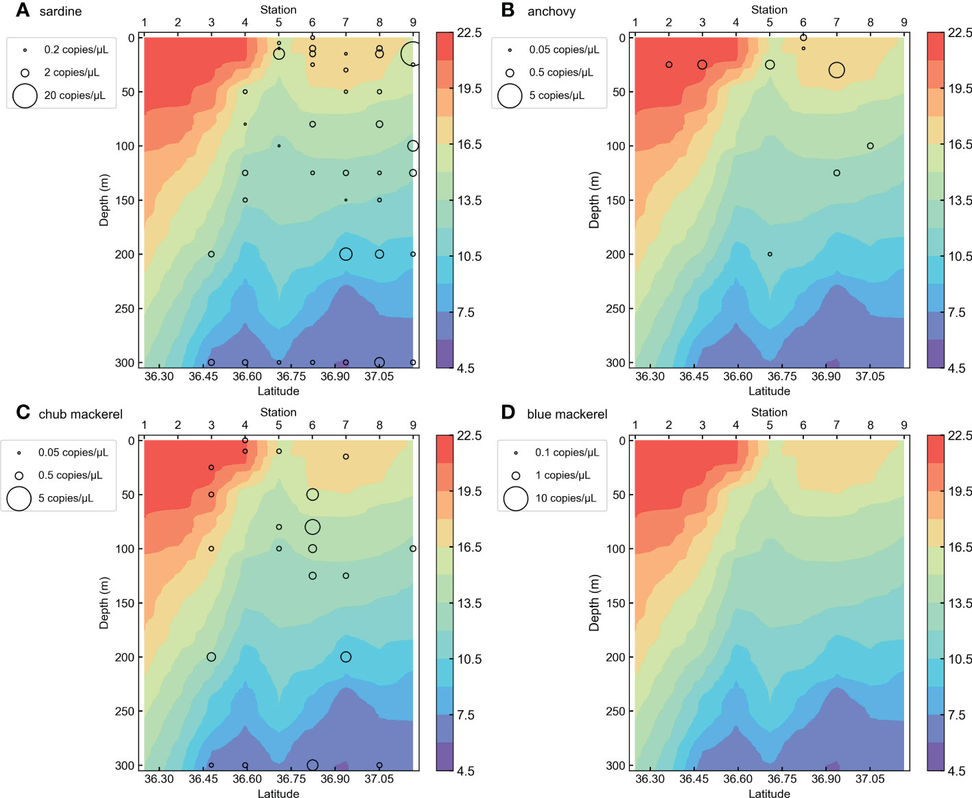
Figure 3 The vertical distribution section of target fish eDNA quantities in KS-18-5 Line-1 for (A) sardine, (B) anchovy, (C) chub mackerel, and (D) blue mackerel. The colors of the background represent sea water temperature recorded during the sampling.

FIGURE 4

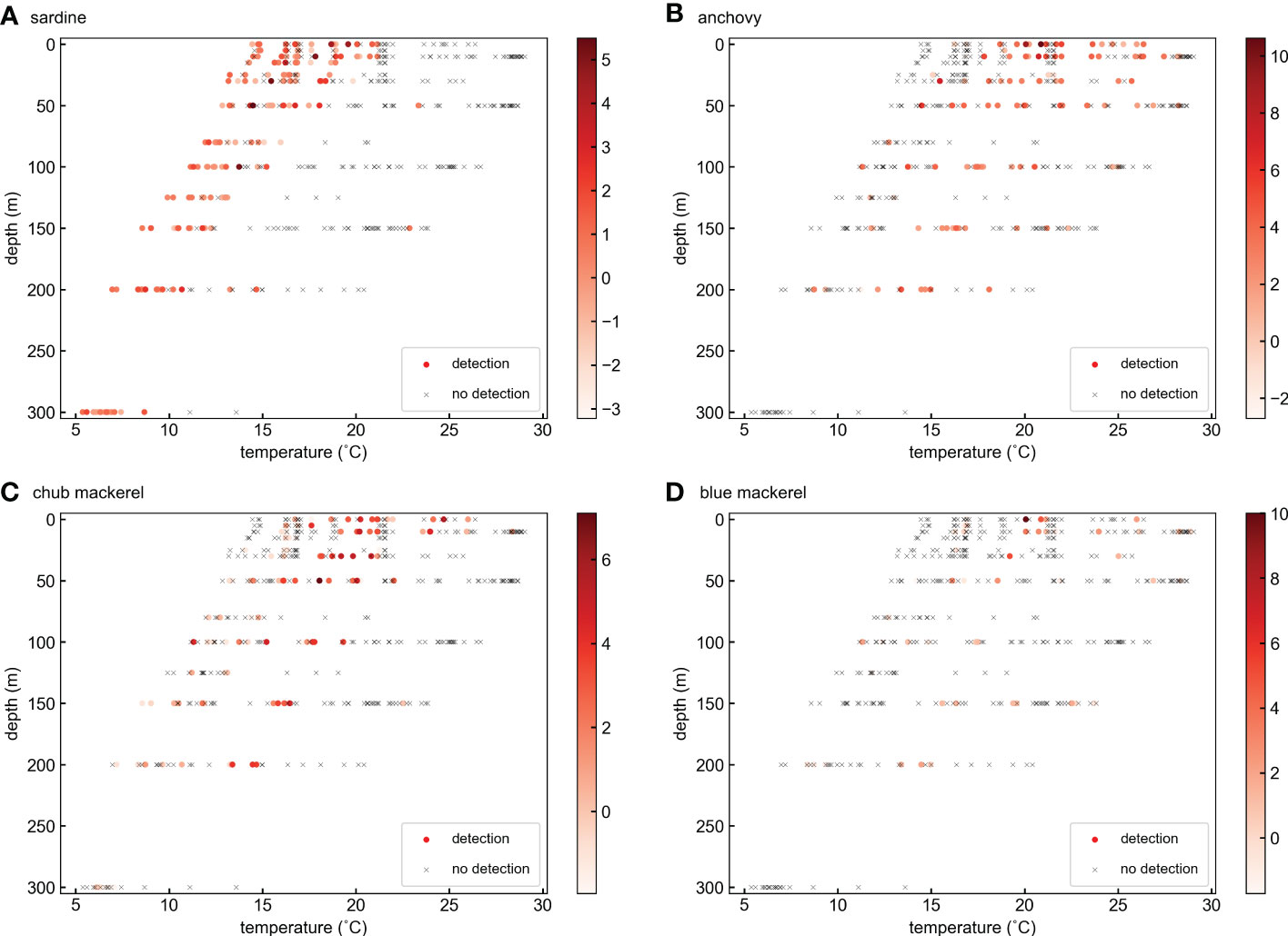
Figure 4 Distribution of target fish DNA at different water temperatures and depths for (A) sardine, (B) anchovy, (C) chub mackerel, and (D) blue mackerel. The colors of ‘○’ markers represent the ln(x) transformed target fish eDNA quantity. The ‘×’ marks represent the samples in which target fish eDNA was not detected.

FIGURE 5

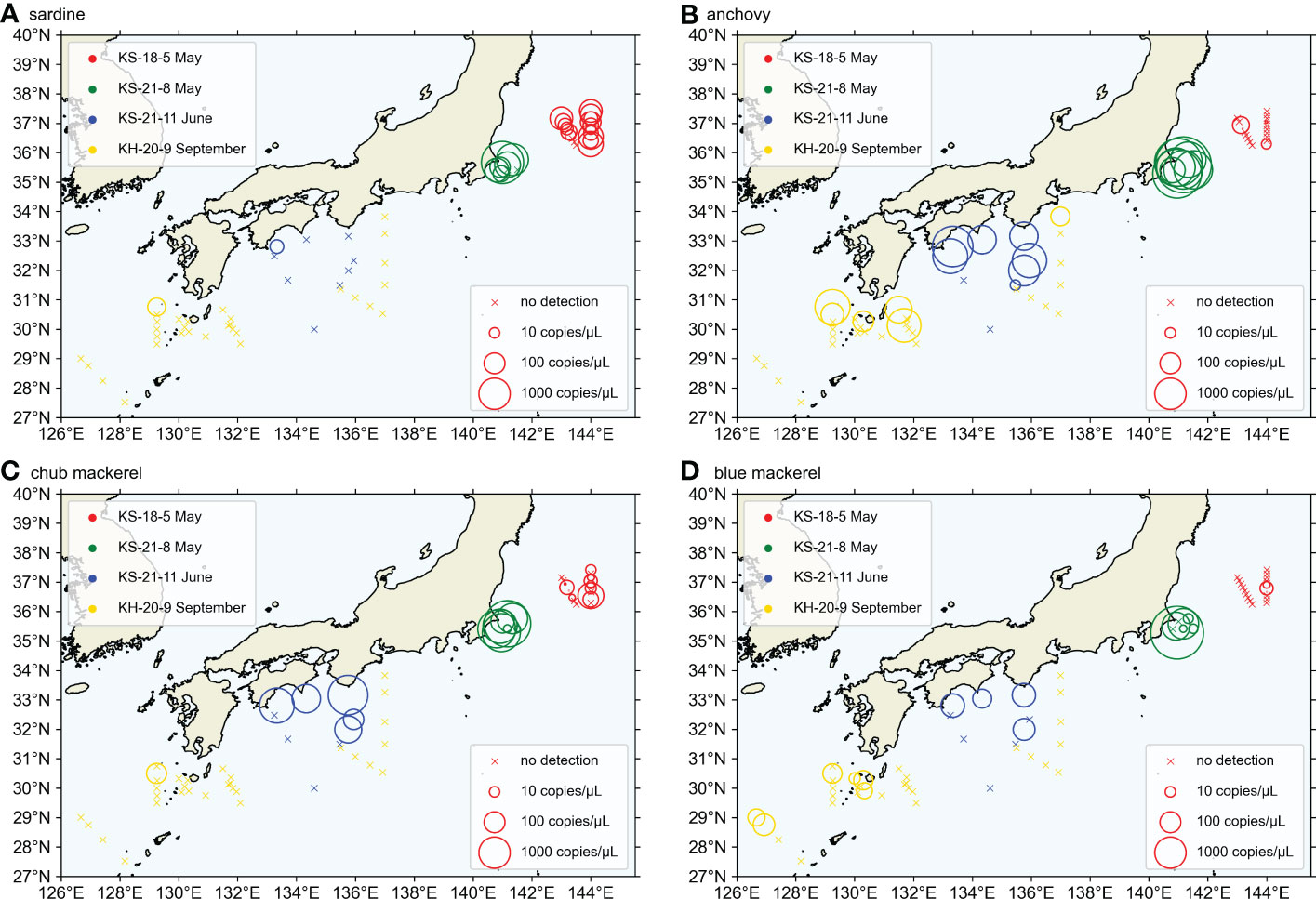
Figure 5 The horizontal distribution of target fish abundance above 60 m depth, represented by eDNA quantity for (A) sardine, (B) anchovy, (C) chub mackerel, and (D) blue mackerel. The abundance above 60 m depth was calculated as the depth-weighted sum of eDNA quantity, like $quantit{y}_{0m}*5+quantit{y}_{10m}*15+quantit{y}_{30m}*20+quantit{y}_{50m}*20$. The sizes of ‘○’ markers represent the target fish eDNA quantity. The ‘×’ marks represent the locations where target fish eDNA was not detected. The stations from different cruises were distinguished by the colors of the ‘○’ and ‘×’ marks.

3.2 Environmental effects on target fish distribution revealed by the first GAM

For the first GAM, which included six CTD-measured environmental factors as explanatory variables, the optimal models for the presence/absence and quantity of the four target fishes (fish quantity was represented by the eDNA quantity) are summarized in Table 1. The partial dependence functions of the explanatory variables that had a significant effect (p<0.05, judged by pyGAM tools, same in the following) in the optimal models are listed in Figures S14–S21.

TABLE 1

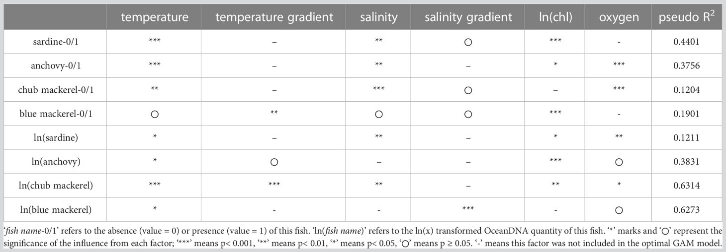
Table 1 The optimal GAM models (derived from the first GAM) showing how environmental factors influence the distribution of each target fish.

Each optimal model included different environmental factors, but only sea water temperature (ranging from 4.5 to 26.5°C here) was included in the optimal models for the presence/absence and quantity of all target fishes (Table 1). Moreover, the effects of temperature were significant in most optimal models except for presence/absence of blue mackerel. Temperature gradient was included in the optimal models for the presence/absence of blue mackerel, and the quantity of anchovy and chub mackerel. Salinity was included in all optimal models except those for the quantity of anchovy and blue mackerel. Salinity gradient was only significant for the quantity of blue mackerel. Chlorophyll-a concentration was included in all optimal models except those for the presence/absence of chub mackerel or the quantity of blue mackerel. Dissolved oxygen concentration was included in all optimal models except those for the presence/absence of sardine and blue mackerel.

Sea temperature showed the most prevalent and significant effect compared to other environmental factors analyzed here. A temperature of 5–12°C had a positive effect on the presence of sardine, whose quantity reached a maximum at 12–21°C (Figures 6A, B). For anchovy, the presence possibility increased as the temperature increased, and the maximum quantity was observed at 21°C (Figures 6C, D). For chub mackerel, the maximum was reached at 19°C, regardless of its presence or quantity (Figures 6E, F). For blue mackerel, both the presence possibility and quantity always increased as temperature increased (Figures 6G, H).

FIGURE 6

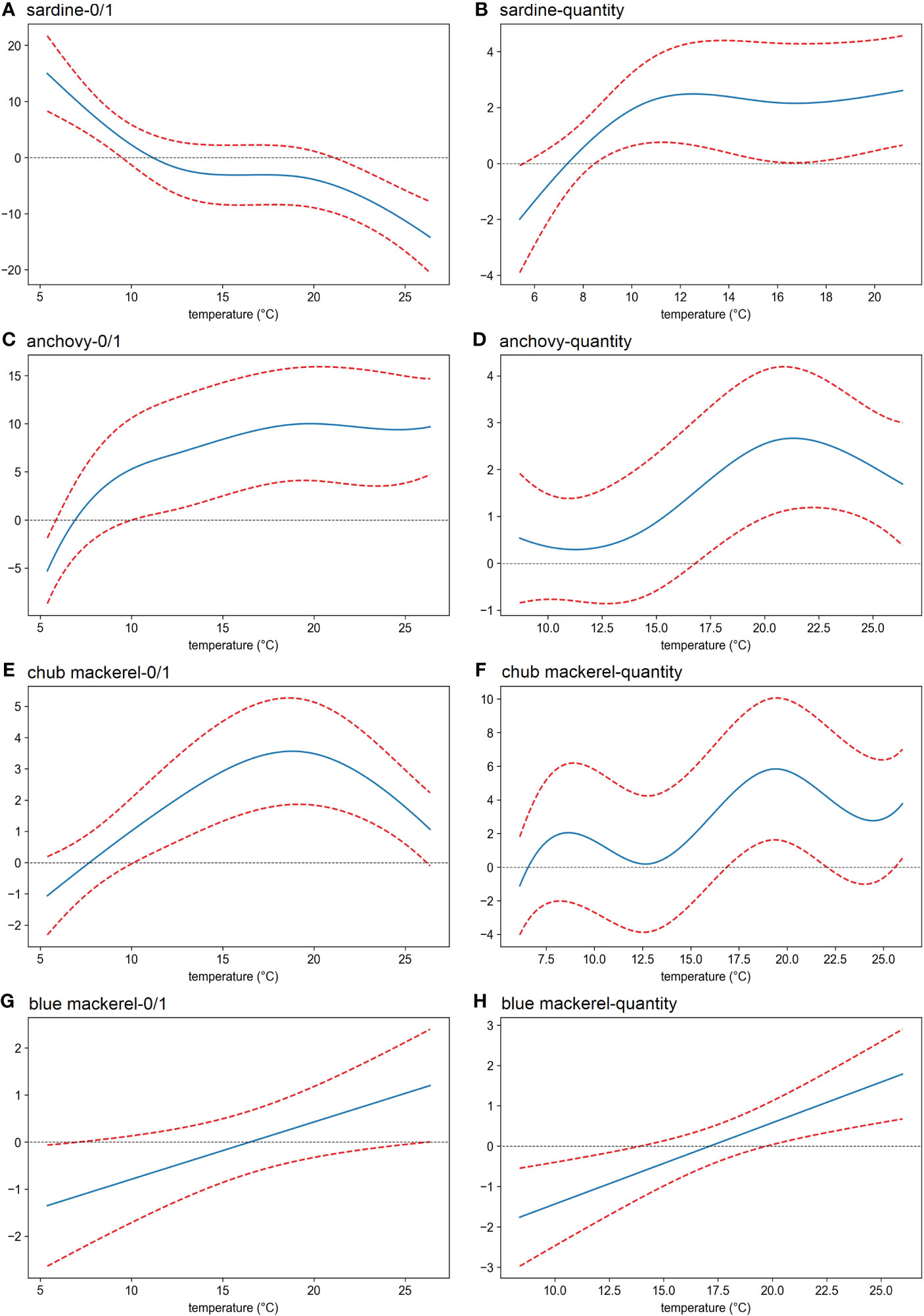
Figure 6 Effects (derived from the first GAM) of sea water temperature on the presence/absence (A, C, E, G) and the eDNA quantity (B, D, F, H) of four target fish. The x-axis shows the value of the explanatory variable (temperature), and the y-axis shows the contribution of the explanatory variable to the fitted values: presence/absence and eDNA quantity of (A, B) sardine (Sardinops melanostictus), (C, D) anchovy (Engraulis japonicus), (E, F) chub mackerel (Scomber japonicus), (G, H) blue mackerel (Scomber australasicus). The area between the two red dotted lines represents the 95% confidence intervals.

Lower salinity generally correlated with an increase of presence or quantity of fishes (Figures S14-S16, S18, S20). Higher chlorophyll-a concentration also correlated with the increase of the presence and quantity of sardine and the quantity of anchovy (Figures S14, S18, S19), whereas it did not show any systematic tendency for the presence of anchovy and blue mackerel and quantity of chub mackerel. Lower dissolved oxygen concentration showed the increase of the presence or quantity of fishes (Figures S15, S16, S18, S20). Stronger salinity gradient showed the quantity increase of blue mackerel (Figure S21).

3.3 Temperature preference indexes of target fish distribution

Given the broad and significant effects of temperature found by the GAM analyses, we further calculated the temperature preference indices of the presence/absence and quantity of each target fish (Figures S27, S28). In the presence of sardine, the TPI was >1 at 4.5–18.5°C, decreasing as the temperature decreased (Figure S27A). In contrast, the preference index increased as the temperature increased in the presence of anchovy (>1 at 18.5–26.5°C, Figure S27B) and blue mackerel (>1 at 16.5–26.5°C, Figure S27D). For the presence of chub mackerel, the TPI had no obvious regularity with temperature change (Figure S27C).

For the quantity of sardine and anchovy the TPI was >1 at 12.5–20.5°C and 18.5–22.5°C, respectively (Figures S28A, B). For the quantity of chub mackerel, the TPI was >1 at 16.5–20.5°C and 22.5–26.5°C (Figure S28C). For the quantity of blue mackerel, the TPI was >1 at 18.5–20.5°C (Figure S28D).

3.4 Environmental effects on the distribution of mackerel revealed by the second GAM

For the second GAM, where we replaced chlorophyll-a concentrations in the explanatory variable list with sardine and anchovy quantities, the optimal models for the presence/absence and quantity of mackerel are summarized in Table 2. The partial dependence functions of the explanatory variables that had significant effects in the optimal models are listed in Figures S22–S25.

TABLE 2

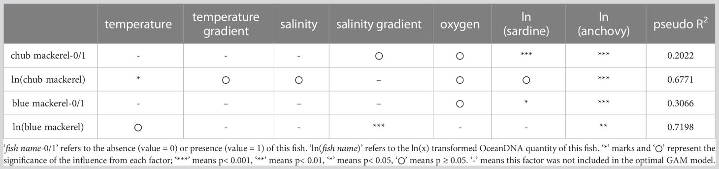
Table 2 The optimal GAM models (derived from the second GAM) showing how environmental factors influence the distribution of mackerels.

Compared with the first GAM, the optimal models of the second GAM showed a higher fitting (higher pseudo R²). The quantity of anchovy and sardine was included in most of the optimal models (Table 2), where the former had significant effects in all optimal models for both chub and blue mackerel (Table 2). Sardine quantity also had significant effects in the optimal models of the presence/absence of the two mackerel (Table 2) but was excluded from the optimal models of blue mackerel quantity, and its effect on chub mackerel quantity was not significant.

For chub mackerel, the presence possibility increased with an increase in either sardine or anchovy quantities (Figures 7A, C). In the case of chub mackerel quantity, the effect of the quantity of sardine and anchovy was more complex (Figures 7B, D). The chub mackerel quantity appeared to increase with an increase in sardine quantity, but the dependency on anchovy quantity had the maximum when anchovy quantity was around 20 copies/μL. In the case of the combined effect of sardine and anchovy quantities, the chub mackerel quantity maximum appeared when the anchovy and sardine eDNA quantity was 20 and 150 copies/μL, respectively (Figure S26). The possibility and quantity of blue mackerel increased with anchovy quantity (Figures 7F, G).

FIGURE 7

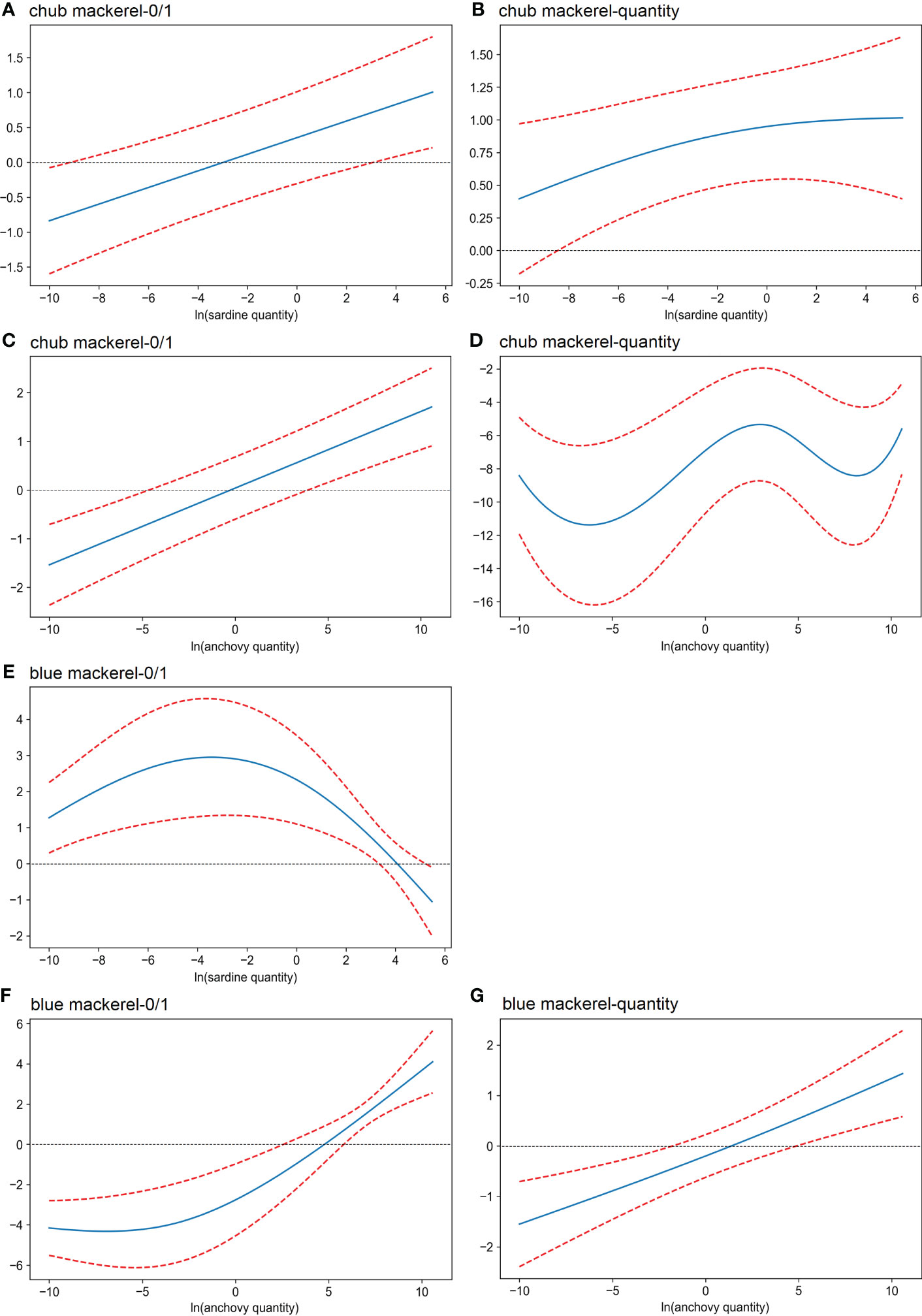
Figure 7 Effects (derived from the second GAM) of the quantity of sardine and anchovy on the presence/absence (A, C, E, F) and the eDNA quantity (B, D, G) of mackerel. The x-axis shows the value of the explanatory variables: (A, B, E) ln(x) transformed sardine quantity; (C, D, F, G) ln(x) transformed anchovy quantity. The y-axis shows the contribution of the explanatory variable to the fitted values: (A, C) presence/absence of chub mackerel; (E, F) presence/absence of blue mackerel; (B, D) ln(x) transformed chub mackerel quantity; (G) ln(x) transformed blue mackerel quantity. The area between the two red dotted lines represents the 95% confidence intervals.

3.5 Distribution difference of target fishes between the inshore and offshore sides of the Kuroshio

In both KS-21-11 and KH-20-9, the average presence percentages of each target fish were higher at the inshore stations (including those on the Kuroshio axis) than the offshore stations (Tables 3, S6). In KS-21-11, the average presence percentage of anchovy was 85.7 and 4.8% among inshore and offshore stations, respectively. In KH-20-9, the average presence percentage of anchovy was 25.0 and 0.0% among inshore and offshore stations, respectively. In the case of blue mackerel, the average presence percentage was 16.7% in KS-21-11 inshore stations, 0.0% in KS-21-11 offshore stations, 21.4% in KH-20-9 offshore stations, and 2.8% in KH-20-9 offshore stations. Moreover, sardine and chub mackerel were only detected at the inshore stations. The Student’s t-test results confirmed the significant difference between the presence percentage of inshore and offshore stations (p< 0.0001, the presence sample percentage data were normally distributed in both KS-21-11 and KH-20-9 samples).

TABLE 3

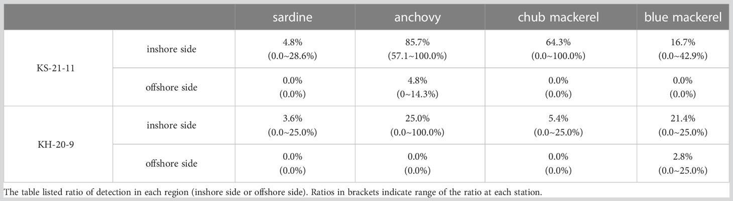
Table 3 The presence sample percentages at inshore (including the Kuroshio axis) and offshore sides of the Kuroshio.

4 Discussion

Here, we analyzed the environment-dependent distribution of four small pelagic fishes in the Kuroshio Current system based on eDNA data, the first study of its kind to our knowledge. By measuring fish eDNA quantity in sea water samples using qPCR, we obtained information on the spatial distribution of the target fishes in this system. We then analyzed the influence of each environmental factor on the target fish distribution, mainly using GAM and preference index analyses. In this section, we discuss our findings and potential limitations of the above analyses.

4.1 The environment-dependent small pelagic fish distribution pattern in the May–June Kuroshio current system

The optimal models produced by the first GAM, revealed how six CTD-measured environmental factors influenced the distribution of four targeted small pelagic fishes (Table 1; Figures S14–21). To simplify the description, we only consider the significant effects on fish occurrence here. The optimal environmental range for sardine to occur included temperature< 12°C, salinity< 34.8 PSU, and chlorophyll-a concentration > 0.14 mg/m³. The optimal environmental range for sardine quantity included temperature > 8°C, salinity< 33.9 PSU, and chlorophyll-a concentration > 0.37 mg/m³. As a result, the optimal environmental range for sardine is regarded as temperature between 8 and 12°C, salinity< 33.9 PSU, and chlorophyll-a concentration > 0.37mg/m³. The optimal environmental range for anchovy to occur included temperature > 6.5°C, salinity< 33.9 PSU, and oxygen concentration< 4.2mL/L. The optimal environmental range for anchovy quantity included temperature > 15.0°C and chlorophyll-a concentration > 1.9 mg/m³. As a result, the optimal environmental range for anchovy is regarded as temperature > 15°C, salinity< 33.9 PSU, and chlorophyll-a concentration > 1.9 mg/m³.

Catch data in the Sea of Japan also indicated the influence of SST and primary production on sardines (Muko et al., 2018). The CPUE distribution in the Yellow and East China Seas was found to be influenced by SST and sea surface salinity (SSS; Liu et al., 2020). A comparison of larval and juvenile growth in the Northwest Pacific showed clear dependency on prey availability for sardine growth but not for that of anchovy, whereas growth of both sardine and anchovy also depended on temperature (Takahashi et al., 2009). Those results are consistent with eDNA derived information on environmental dependency. The eDNA sampling is relatively simple and enables high horizontal and vertical resolution fish distribution observation corresponding to the environment. Our results support the possibility of using eDNA to better understand the relationship between fish species distribution and environments.

4.2 The role of sea water temperature in target fish distribution

For sardine and anchovy, significant effects of sea water temperature on the occurrence and quantity of eDNA were revealed (Table 1). Moreover, as temperature-dependent patterns derived from GAM and TPI analyses were always similar (e.g., Figures 6A vs. S27A; 6C vs. S27B), it can be concluded that sea water temperature was a decisive factor influencing the distribution of sardine and anchovy in the Kuroshio Current system. In addition, our results showed the different temperature preferences where anchovies preferred warm water while sardines preferred cooler environments.

Differences in temperature preferences of sardine and anchovy have been noted in previous studies, and a hypothesis on the different temperature responses to explain the alternations between the two species was proposed (Takasuka et al., 2007; Takasuka et al., 2008b; Itoh et al., 2009). For example, otolith analysis by Takasuka et al. (2007) showed that anchovy and sardine larvae had the highest growth rate at 22.0 and 16.2°C, respectively. They also found that the preferred spawning temperatures of the two species (Takasuka et al., 2008b) had the same temperature dependence difference. As GAM analyses decomposed and inspected the contribution of each feature, our study supported this hypothesis by providing clearer evidence for the effects of temperature on the distribution of sardine and anchovy.

For chub and blue mackerel, researchers have also studied the relationship between temperature and their distribution. For example, larval sampling in the southern East China Sea by Sassa and Tsukamoto (2010) showed that the habitat temperature range of blue mackerel larvae was higher and narrower than that of chub mackerel, which was consistent with the distribution pattern revealed when sardine and anchovy quantity information was not considered (Figures 6E vs. 6G; 6F vs. 6H). However, our results suggest that the influence of temperature on the distribution of mackerel is less decisive. Although the GAM and TPI analyses for blue mackerel occurrence showed similar trends (Figure 6G vs. S27D), this temperature effect was not significant (Table 1). Moreover, for blue mackerel quantity as well as chub mackerel occurrence, the GAM and TPI analyses did not find the same temperature-dependent pattern. Thus, we speculated that temperature may not be the most important factor in determining the mackerel distribution—other factors are also involved, such as the anchovy and sardine quantity effects which will be discussed further in the next section (Section 4.3). In fact, the results of our study have revealed that the temperature is less effective in determining mackerel distribution when sardine and anchovy quantity information is considered (see Section 3.4).

Sea water temperature not only changes with horizontal position but also usually decreases with depth. Therefore, it is possible that the effects of temperature deduced from the GAM included the effects of preferred habitat layer differences among species. Sardine and anchovy have different temperature preferences, as shown in the GAM analysis. Indeed, for the occurrence of these fishes, the vertical distribution pattern deduced from eDNA data (Figure S29) partially revealed a mirrored structure. However, in terms of eDNA quantity, all target fishes were concentrated in the water layer at 0–50 m depth (Figure S30), which did not explain the temperature preference of the target fishes (Figure S28). An earlier study also did not support the hypothesis that sardine and anchovy prefer to stay at different depths (Yatsu et al., 2005). Indeed, the distribution of target fish eDNA on the water temperature and depth plane (Figure 4) revealed the significant temperature effects on the distribution of sardine and anchovy. The occurrence of sardine eDNA was obviously concentrated at cooler temperatures regardless of depth.

However, the temperature range shifts to cooler with depth. Because sardine larvae are distributed mainly in the surface layer shallower than 50 m (Hayashi, 1990; Matsuo et al., 1997), the temperature range shift might reflect the different temperature preferences of sardine in different life stages. Because a high eDNA quantity appeared more often in the layers shallower than 50 m, it follows that it appeared between 14 and 20°C. These characteristics are consistent with the GAM results (Figures 6A, B). The occurrence of anchovy eDNA was mainly distributed in the warmer temperature range compared with that of sardine in all depth layers (Figure 4B). In addition, the samples with high anchovy eDNA quantities mainly appeared when the water temperature was 21°C above 50 m depth (Figure 4B). These characteristics are also partially consistent with the GAM results (Figures 6C, D). Thus, we suggest that the temperature effects deduced from the GAM analyses mostly reflect the temperature preferences of the target fishes. However, because the eDNA methods are unable to distinguish different body sizes or life stages in the same species, the GAM-deduced temperature effect for one species might be evaluating the overall water temperature preferences of a fish group that includes different life stages. Special caution is needed for this issue, as discussed in Section 4.5.

The fishing catch can provide direct information on fish, including species, abundance, size, and life history. However, the use of scientific fishing surveys has been limited, especially in the open ocean. The research vessels included in this study also did not have equipment such as large nets for fishing. Acoustic sonar, another technology used for fish surveys, can measure fish size and abundance (Medwin and Clay, 1998; Boswell and Wilson, 2011) but cannot accurately distinguish fish species. Moreover, with the prior knowledge from fishing, it is possible to judge the life history stage from fish size. Therefore, in the future survey, we suggest combining the use of eDNA with other methods such as acoustic sonar (and fishing, if possible), to provide more accurate data on small pelagic fish distribution patterns.

4.3 Anchovy and sardine quantity effects on mackerel distribution patterns

Abiotic environmental factors, such as temperature, together with chlorophyll-a concentration (or primary production), have long been used to analyze the distribution patterns and estimate the habitat areas of small pelagic fishes, including chub and blue mackerel (Chen et al., 2009; Li et al., 2014; Lee et al., 2018; Yu et al., 2018). Conversely, although researchers have recognized the piscivorous habits of chub and blue mackerel (Yoon et al., 2008; Robert et al., 2010), prey fish have not yet been considered as influencing factors in their distribution patterns.

Mackerel (chub and blue) are piscivorous fishes (Robert et al., 2010) whose main prey is anchovy (Nakatsuka et al., 2010; Robert et al., 2010). Our results suggest an influence of anchovy and sardine quantity on the distribution patterns of chub and blue mackerel in the Kuroshio Current system. Indeed, abiotic environmental factors, including temperature (Table 2), as well as chlorophyll-a concentration (Table 1), appeared less influential when compared with sardine and anchovy eDNA levels, especially anchovy (Table 2). The results revealed anchovy-dependent patterns in chub and blue mackerel distributions in that as the density of anchovy increased, the possibility of the presence and density of mackerel increased (Figures 7, S26). Based on our data, the estimated blue mackerel quantity (derived from the GAM) increased more than seven times when the anchovy quantity increased from the minimum to the maximum (Figure 7). Higher anchovy quantities also had a positive effect on chub mackerel quantity (Figures 7, S26).

However, eDNA method does not detect the fish size or life stage, and capturing larger mackerel which has high swimming speed is difficult. Indeed, the Shinsei-Maru and Hakuho-Maru research vessels are unable to conduct a large size net survey. Thus, we did not collect any fish body samples. Therefore, direct information about predation, such as the stomach content of mackerels, was not available. However, considering anchovy is the main prey of mackerel (Nakatsuka et al., 2010; Robert et al., 2010), it might be hypothesized that the GAM results indicate prey-predator interaction between anchovy and mackerel. In the offshore waters, between the Kuroshio Extension and Oyashio Front (mixed water region), distribution temperature overlapped between anchovy and chub mackerel in early summer (Fuji et al., 2023), which was confirmed by a surface trawl survey. Nakatsuka et al. (2010) confirmed anchovy in the stomach contents of chub mackerel in the mixed water region. Those results support our hypothesis that mackerel distribution depends on anchovy because mackerel prey on anchovy. However, this is still a hypothesis and there are other possible explanations, such as that the mackerel and anchovy came to the same place to predate on the same kind of zooplankton. Therefore, a future study combining the eDNA survey with a net survey is recommended.

Even if we know the prey-predator relationship, it is difficult to investigate the influence of prey fishes on predator fish distribution because of the lack of distribution data for both these fish types. Studies on the effect of prey fishes on fish distribution have been limited to large predators such as tuna (Schick and Lutcavage, 2009; Lezama-Ochoa et al., 2010) and Spanish mackerel (Liu et al., 2023). Most habitat models for fish distribution have used satellite-derived data that can cover wide spatial-temporal scales. Our results indicate the effectiveness of eDNA in investigating predator–prey overlap and interactions and also suggest that there is a great need to analyze the role of prey fish, seldom thought to be an influence in the distribution of piscivorous fishes (Pepin et al., 1987; Cabral and Murta, 2002; Emmett and Krutzikowsky, 2011). The predator–prey overlap shown by eDNA, combined with the data from other methods like stomach content analysis, can improve the understanding of the relationship between prey fish and the distribution of piscivorous fishes. The collaboration of eDNA with other methods can also help with the study of the diet selectivity of the predator. The typical idea to analyze diet selectivity is to compare diet composition in the stomach content with prey availability (Pine et al., 2005). This analysis needs the distribution of prey species around the predator, which could be more easily obtained by the eDNA method.

4.4 Small pelagic fish distribution differences between inshore and offshore sides of the Kuroshio

In addition to the environmental factors discussed above, this study also tested the “barrier effect” of the Kuroshio on the distribution of our targeted small pelagic fishes. Our results showed that anchovy, chub mackerel, and blue mackerel were significantly more abundant on the inshore side of the Kuroshio (or on the Kuroshio axis) than on the offshore side (Tables 3, S6). The occurrence of these target fishes decreased suddenly or even disappeared in the offshore side (Tables 3, S6). Despite of its low occurrence, sardine was only detected on the inshore side. Our eDNA sampling indicated the “barrier effect” of the Kuroshio on the distribution of the small pelagic fishes.

The distribution characteristics were consistent with those reported in previous studies. Nishikawa et al. (2022) suggested that the environmental condition (temperature and Chl-a concentration) on the inshore side/axis of the Kuroshio is suitable for sardine and anchovy larvae. It was shown that chub mackerel larvae on the northern (inshore) side of the Kuroshio axis have better growth chances (Higuchi et al., 2019; Sogawa et al., 2019; Guo et al., 2022). The first GAM results showed a lower salinity preference in the presence of sardine, anchovy, and chub mackerel (Figures S14-16) as well as the quantity of sardine and chub mackerel (Figures S18, 20). The inshore side of the Kuroshio axis has lower salinity than the offshore side; therefore, this lower salinity preference tendency corresponds to a higher abundance of the small pelagic fishes in the inshore side of the Kuroshio.

Zooplankton are an important food source for small pelagic fishes; therefore, the different distributions of zooplankton (Watanabe et al., 2002; Miyamoto et al., 2017) on the two sides of the Kuroshio axis could be one of the reasons for the different distributions of fish. For example, Miyamoto et al. (2017) found that in zooplankton samples, copepod abundance was highest in the north-frontal area of the Kuroshio. To clarify whether the different distributions of zooplankton caused the different distributions of fish on the two sides of the Kuroshio axis, a simultaneous and co-located distribution information of fish and zooplankton are needed, which can be provided by the eDNA method. For example, Minegishi et al. (2023) simultaneously measured the spatiotemporal distribution of chum salmon (Oncorhynchus keta) eDNA as well as the eDNA of its three zooplankton prey (Pseudocalanus newmani, Eucalanus bungii, and Themisto japonica) in the Otsuchi Bay, using the same water samples. Similarly, by simultaneously measuring the distribution of targeted small pelagic fish and their zooplankton prey (e.g., the species found in fish stomach contents) in the Kuroshio, we expect the eDNA method can be helpful in clarifying the reasons of fish distribution difference between the two sides of the Kuroshio axis. However, the reasons for this difference remain unclear and the possible influence of other factors (such as water current velocity) cannot be ignored, necessitating further research for any possible reasons in the future.

4.5 Seasonal difference of small pelagic fish distribution patterns

The sections above have discussed the environment-dependent distribution patterns of the small pelagic fishes that were observed in this study. Those analyses on the effects of six CTD-measured environmental factors and the potential prey fish on the small pelagic fish distribution were all based on samples from three cruises during May–June (KS-18-5, KS-21-8, and KS-21-11). However, the environmental conditions and the fish distribution in the ocean may vary among different seasons. We wanted to compare the distributional characteristic of the small pelagic fishes in September. But, in KH-20-9, the detection of small pelagic fishes was limited to 2, 16, 3, and 13 for sardine, anchovy, chub and blue mackerel, respectively. The presence data was too few to conduct GAM analyses. Therefore, this study could not evaluate seasonal variability of distributional characteristics of the small pelagic fishes. Especially, September is not active spawning season for the target fishes, which may alter the environmental dependency of the fish distribution. Thus, we need to suggest that the dependency of the small pelagic fish distribution on environments and potential prey fish, we revealed in this study, may only be representative in certain seasons or for fish in certain ontogenetic stages. The comprehensive understanding of the distribution pattern of these fishes requires more study in the future.

4.6 Limitations and challenges of eDNA on fish distribution surveys

Being non-invasive and having low energy consumption (compared with traditional trawling sampling), eDNA methods have been actively used in fish surveys. Even so, as eDNA methods cannot directly observe individual fish, there are several limitations and challenges in eDNA observation for detecting fish distribution.

The first concerns the adequacy of using eDNA quantity to represent fish quantity. Many previous studies have shown notable positive correlations between eDNA concentration and fish biomass or number of individuals in aquarium experiments (Takahara et al., 2012; Doi et al., 2015; Horiuchi et al., 2019). In addition, by comparing eDNA data with data from other survey methods, similar relationships have also been recorded in field surveys in large natural waters (Yamamoto et al., 2016; Minegishi et al., 2019; Salter et al., 2019). For example, Salter et al. (2019) found significantly positive correlations (p = 0.003) between the trawl-biomass and eDNA quantity of Atlantic cod (Gadus morhua) in oceanic waters around the Faroe Islands. Therefore, the idea to represent fish quantity by eDNA quantity has its rationale. However, because the proportionality coefficient between eDNA concentration and abundance is species-specific, it is not possible to compare the relative abundance of fish species by eDNA concentration. Additional laboratory experiments and field data comparisons are essential for developing methods for estimating fish abundance using eDNA.

The second is the spatio-temporal representativeness of eDNA data. After being released into water, eDNA remains detectable for a while during which time it may move to other places. In one field experiment by Murakami et al. (2019) using caged fish at the sea surface in Maizuru Bay (Kyoto, Japan), it was found that eDNA was only detectable<2 h after release and mostly found within 30 m horizontally and 4 m vertically from the fish cage (Murakami et al., 2019). Other studies also suggested that the spread of eDNA was limited from the release point both horizontally (O'Donnell et al., 2017; Yamamoto et al., 2016) within 100–150 m and vertically (Yamamoto et al., 2016; Jeunen et al., 2019; Littlefair et al., 2020) within 5–30 m. These studies support the idea that eDNA is swiftly degraded and not advected far from the fish; therefore, we considered that eDNA distributions represent fish distributions. However, since degradation time depends on temperature and species, and the advected distance depends on the current speed, more studies on the degradation and transportation of eDNA are necessary, like those by Tsuji et al. (2017); Saito and Doi (2021), and Murakami et al. (2019). In addition, knowledge regarding eDNA sedimentation is limited. Although the modeling performed by Allan et al. (2021) suggested that settling, as well as other physical processes such as mixing and advection, only caused a 10–20m vertical displacement, more fieldwork data is needed to truly understand the vertical space accuracy of eDNA signals.

Another problem with eDNA methods is the inability to determine whether the DNA originates from a living individual. Thus, carcasses, or even DNA left in predator feces (Parsons et al., 2006; Deagle et al., 2009), may become unexpected eDNA sources and result in false-positive detections. For example, the sardine DNA signals we found in several 300 m water samples (Table S5 and Figure 3A) may have come from the eDNA source that sank from the upper layer. Because of gravity, large carcass pieces or feces sink quickly rather than remaining in a certain water layer, so they are likely to gather at the sea bottom. However, the sea bottom is much deeper than where we collected our samples at most of the stations (e.g., the sea bottom depth of stations in Line 1 is deeper than 5000 m; Table S1), so the large pieces of eDNA on the sea bottom are not likely to contribute to the eDNA of our samples, except for KS-21-8 Lines 3 and 4 and KH-20-9 Line 8. The effect of the sea bottom was not obvious in KS-18-5 Lines 1 and 2. The smaller particles from carcasses or predator feces are also likely to suspend and aggregate in the pycnocline, where the vertical water density gradient is high. However, neither temperature nor salinity gradients were included as significant influencing factors in the optimal GAM models for the eDNA distribution of either sardine or anchovy (Table 1, Figures S14, 15, 18, 19). Indeed, an extremely high eDNA quantity was not detected in the thermocline layer in all the vertical sections. In KS-18-5 Lines 1 and 2, where water samples were collected at 300 m, sardine were detected even at that depth. Because the temperature gradient was not high in the layer (Figures 3, S1), it was difficult to consider the eDNA aggregates there. As mentioned above, sardine larvae are concentrated above 50 m, but there is also a sardine egg record at a depth of 300 m (Hayashi, 1990). Therefore, we could not conclude that the eDNA at 300 m originated from this layer. Prior knowledge of this problem is limited and inconsistent. For example, Kamoroff and Goldberg (2018) found that goldfish (Carassius auratus) carcasses in tanks produced detectable eDNA, but less than that from live goldfish. In contrast, Curtis and Larson (2020) found that crayfish (Procambarus clarkii) carcasses in streams did not produce any detectable eDNA. Therefore, we did not consider eDNA sources other than those from live fish here, but we suggest that further research is needed on the contribution of fish carcasses or predator feces as eDNA sources, in terms of their transportation in the ocean and how much DNA they produce.

Finally, there is another limitation when performing eDNA analysis on fish rather than on microorganisms. A suitable environment for a fish can vary with its growth and development (Fernández-Corredor et al., 2021), but its eDNA is unable to deliver information on its body size or life stages. Thus, the results of our study may combine the environmental preferences of larvae and adults of the same fish species. As mentioned in Section 4.2, we found that the temperature range preference of sardine appeared to shift to cooler as the depth increased (Figure 4A), whereas the warmer temperature preference of anchovy was not obvious in layers deeper than 100 m (Figure 4B). One possible explanation for this phenomenon is that eDNA signals on the surface mainly originated from larvae and juveniles, while those in deeper layers mainly originated from adult fish, and, in our case, the sardine and anchovy adults were better adapted to lower temperatures than their larvae and juveniles. Previous studies on related species have supported this assumption. For example, Boyra et al. (2016) found that juvenile anchovy (E. encrasicolus) in the French sector of the Bay of Biscay moved from above 50 m to 100 m depth or deeper (where it is also much cooler) as they grow. Similarly, as eDNA cannot tell us whether the mackerel were large enough to prey on the anchovy within the same area, we cannot deduce whether the prey-predator relationship actually existed. We can only deduce the relationship between prey fish and the distribution pattern of chub mackerel and blue mackerel based on eDNA data, like we have discussed in Section 4.3. Although the inability to distinguish fish sizes and life history stages limits the accuracy of the fish distribution pattern derived from eDNA data, researchers have not developed a solution for this problem in eDNA methods. Using a newly developed technology called environmental RNA (eRNA), which detects RNA released by organisms into the environment (Cristescu, 2019), it is possible to estimate the physiological status of target organisms (Tsuri et al., 2020). Therefore, combining eRNA with eDNA may be a potential way to distinguish the different life stages of fish. Conversely, as fish catches can provide direct information about their size and life history stages and acoustic sonar is also able to measure fish sizes (Rudstam et al., 1987), combining traditional and mature survey methods such as net sampling and acoustic sonar with eDNA methods may be another feasible solution to upgrade the accuracy of eDNA survey data. However, further efforts are needed to overcome the limitations of eDNA methods for fish surveys.

5 Conclusion

This study researched the environment-dependent distribution patterns of four small pelagic fishes, sardine, anchovy, chub mackerel, and blue mackerel, in the Kuroshio Current system based on eDNA data. The GAM revealed the diverse relationships of target fishes with the environment, which showed the influence of multiple environmental factors, such as sea water temperature, salinity, dissolved oxygen concentration, and chlorophyll-a concentration. Among the four target fish species, the influence of sea water temperature was especially decisive for the distribution of sardine and anchovy, and the different temperature preferences of sardine and anchovy—that sardine prefers cooler water than anchovy—were supported by the results of this study. Our results suggest the distributions of chub and blue mackerel are highly dependent on anchovy and sardine quantities in the Kuroshio Current system, and we hypothesized that a prey-predator relationship between anchovy and mackerel influenced the mackerel distribution. We emphasized the necessity to consider prey fish effects when investigate piscivorous fish distribution. In addition, the comparison of target fish eDNA data between the two sides of the Kuroshio axis in this study showed the concentrated distribution of all target fishes in the inshore side and confirmed the “barrier effect” of the Kuroshio on the small pelagic fishes.

Data availability statement

The original contributions presented in the study are included in the article/Supplementary Material. Further inquiries can be directed to the corresponding author.

Ethics statement

Ethical review and approval was not required for the animal study because we investigated only enviromental DNA sampled from sea waters.

Author contributions

ZY and S-II contributed to the study conception and design. ZY, S-II, MW, JI, SI, KK, SA and TH curated data. ZY, MW, TH, and SH performed statistical analyses. ZY, S-II, JI, SI, KK, HS and SA participated in the study. S-II, SI, SH and HS administered the study. ZY wrote the first draft of the manuscript. All authors contributed to the manuscript revision and read and approved the submitted version.

Funding

S-II, JP21H04735, and JP22H05030. The Japan Society for the Promotion of Science (JSPS) KAKENHI, https://www.jsps.go.jp/english/. The funders had no role in the study design, data collection and analysis, decision to publish, or manuscript preparation. S-II and SH, The OceanDNA Project, The University of Tokyo Future Society Initiative, https://www.u-tokyo.ac.jp/adm/fsi/ja/projects/sdgs/projects_00103.html. The funders had no role in the study design, data collection and analysis, decision to publish, or manuscript preparation.

Acknowledgments

The OceanDNA survey was conducted by the research vessels Shinsei-Maru and Hakuho-Maru. We thank the captains and all members of the cruises KS-18-5, KS-21-8, KS-21-11, and KH-20-9. We also appreciate the assistance of Dr. Megumi Enomoto in sea water sampling. We express special thanks to Mr. Shinsuke Toyoda, Mr. Hironori Sato, Mr. Yo Watanabe, and Mr. Minoru Kamata of Marine Work Japan for their assistance with the CTD water sampling device. We deeply appreciate the contribution devoted to the observational and analytical support provided by Ms. Kiriko Ikeba.

Conflict of interest

The authors declare that the research was conducted in the absence of any commercial or financial relationships that could be construed as potential conflicts of interest.

Publisher’s note

All claims expressed in this article are solely those of the authors and do not necessarily represent those of their affiliated organizations, or those of the publisher, the editors and the reviewers. Any product that may be evaluated in this article, or claim that may be made by its manufacturer, is not guaranteed or endorsed by the publisher.

Supplementary material

The Supplementary Material for this article can be found online at: https://www.frontiersin.org/articles/10.3389/fmars.2023.1121088/full#supplementary-material

References

Alheit J., Licandro P., Coombs S., Garcia A., Giráldez A., Santamaría M. T. G., et al. (2014). Reprint of “Atlantic multidecadal oscillation (AMO) modulates dynamics of small pelagic fishes and ecosystem regime shifts in the eastern north and central atlantic”. J. Mar. Syst. 133, 88–102. doi: 10.1016/j.jmarsys.2014.02.005

CrossRef Full Text | Google Scholar

Ali M. A., Gyulai G., Hidvégi N., Kerti B., Al.Hemaid F. M., Pandey A. K., et al. (2014). The changing epitome of species identification – DNA barcoding. Saudi. J. Biol. Sci. 21, 204–231. doi: 10.1016/j.sjbs.2014.03.003

PubMed Abstract | CrossRef Full Text | Google Scholar

Allan E. A., DiBenedetto M. H., Lavery A. C., Govindarajan A. F., Zhang W. G. (2021). Modeling characterization of the vertical and temporal variability of environmental DNA in the mesopelagic ocean. Sci. Rep. 11. doi: 10.1038/s41598-021-00288-5

CrossRef Full Text | Google Scholar

Ambe D., Imawaki S., Uchida H., Ichikawa K. (2004). Estimating the kuroshio axis south of Japan using combination of satellite altimetry and drifting buoys. J. Oceanogr. 60, 375–382. doi: 10.1023/B:JOCE.0000038343.31468.fe

CrossRef Full Text | Google Scholar

Barnes M. A., Turner C. R. (2016). The ecology of environmental DNA and implications for conservation genetics. Conserv 17, 1–17. doi: 10.1007/s10592-015-0775-4

CrossRef Full Text | Google Scholar

Boswell K. M., Wilson M. P., Cowab J. H. Jr. (2011). A semiautomated approach to estimating fish size, abundance, and behavior from dual-frequency identification sonar (DIDSON) data. N. Am. J. Fish. Manag. 28, 799–807. doi: 10.1577/M07-116.1

CrossRef Full Text | Google Scholar

Boyra G., Peña M., Cotano U., Irigoien X., Rubio A., Nogueira E. (2016). ). spatial dynamics of juvenile anchovy in the bay of Biscay. Fish. Oceanogr. 25, 529–543. doi: 10.1111/fog.12170

CrossRef Full Text | Google Scholar

Brochier T., Echevin V., Tam J., Chaigneau A., Goubanova K., Bertrand A. (2013). Climate change scenarios experiments predict a future reduction in small pelagic fish recruitment in the Humboldt current system. Glob. Chang. Biol. 19, 1841–1853. doi: 10.1111/gcb.12184

PubMed Abstract | CrossRef Full Text | Google Scholar

Brosset P., Fromentin J., Beveren E. V., Lloret J., Marques V., Basilone G. (2017). Spatio-temporal patterns and environmental controls of small pelagic fish body condition from contrasted Mediterranean areas. Prog. Oceanogr. 151, 149–162. doi: 10.1016/j.pocean.2016.12.002

CrossRef Full Text | Google Scholar

Bunce M., Szulkin M., Lerner H. R., Barnes I., Shapiro B., Cooper A., et al. (2005). Ancient DNA provides new insights into the evolutionary history of new zealand's extinct giant eagle. PloS Biol. 3, 14–23. doi: 10.1371/journal.pbio.0030009

CrossRef Full Text | Google Scholar

Cabral H. N., Murta A. G. (2002). The diet of blue whiting, hake, horse mackerel and mackerel off Portugal. J. Appl. Ichthyol. 18, 14–23. doi: 10.1046/j.1439-0426.2002.00297.x

CrossRef Full Text | Google Scholar

Chen X., Li G., Bo F., Tian S. (2009). Habitat suitability index of chub mackerel (Scomber japonicus) from July to September in the East China Sea. J. Oceanogr. 65, 93–102. doi: 10.1007/s10872-009-0009-9

CrossRef Full Text | Google Scholar

Cristescu M. E. (2019). Can environmental RNA revolutionize biodiversity science? Trends Ecol. Evol. 34, 694–697. doi: 10.1016/j.tree.2019.05.003

PubMed Abstract | CrossRef Full Text | Google Scholar

Curtis A. N., Larson E. R. (2020). No evidence that crayfish carcasses produce detectable environmental DNA (eDNA) in a stream enclosure experiment. PeerJ 8, 603–618. doi: 10.7717/peerj.9333

CrossRef Full Text | Google Scholar

Cury P. M., Boyd I. L., Bonhommeau S., Anker-Nilssen T., Crawford R. J. M., Furness R. W., et al. (2011). Global seabird response to forage fish depletion–One-Third for the birds. Science 334, 1703–1706. doi: 10.1126/science.1212928

PubMed Abstract | CrossRef Full Text | Google Scholar

Cury P., Cury A., Crawford R., Jarre A., Quinãones R., Shannon L., et al. (2000). Small pelagics in upwelling systems: patterns of interaction and structural changes in “wasp-waist” ecosystems. ICES. J. Mar. Sci. 57, 603–618. doi: 10.1006/jmsc.2000.0712

CrossRef Full Text | Google Scholar

Deagle B. E., Kirkwood R., Jarman S. N. (2009). Analysis of Australian fur seal diet by pyrosequencing prey DNA in faeces. Mol. Biol. 18, 2022–2038. doi: 10.1111/j.1365-294X.2009.04158.x

CrossRef Full Text | Google Scholar

Doi H., Uchii K., Takahara T., Matsuhashi S., Yamanaka H., Minamoto T. (2015). Use of droplet digital PCR for estimation of fish abundance and biomass in environmental DNA surveys. PloS One 10. doi: 10.1371/journal.pone.0122763

PubMed Abstract | CrossRef Full Text | Google Scholar

Duarte L. O., Garcıía C. B. (2004). Trophic role of small pelagic fishes in a tropical upwelling ecosystem. Ecol. Modell. 172, 323–338. doi: 10.1016/j.ecolmodel.2003.09.014

CrossRef Full Text | Google Scholar

Emmett R. L., Krutzikowsky G. K. (2011). Nocturnal feeding of pacific hake and jack mackerel off the mouth of the Columbia river 1998-2004: implications for juvenile salmon predation. Trans. Am. Fish. Soc. 137, 657–676. doi: 10.1577/T06-058.1

CrossRef Full Text | Google Scholar

ESR (2009). OSCAR third deg. ver. 1. PO.DAAC (CA, USA). doi: 10.5067/OSCAR-03D01

CrossRef Full Text | Google Scholar

Everts T., Driessche C. V., Neyrinck S., Regge N. D., Descamps S., Vocht A. D., et al. (2022). Using quantitative eDNA analyses to accurately estimate American bullfrog abundance and to evaluate management efficacy. Environ. DNA. 4, 1052–1064. doi: 10.1002/edn3.301

CrossRef Full Text | Google Scholar

Fernández-Corredor E., Albo-Puigserver M., Pennino M. G., Bellido J. M., Coll M. (2021). Influence of environmental factors on different life stages of European anchovy (Engraulis encrasicolus) and European sardine (Sardina pilchardus) from the Mediterranean Sea: a literature review. Reg. Stud. Mar. Sci. 41. doi: 10.1016/j.rsma.2020.101606

CrossRef Full Text | Google Scholar

Food and Agriculture Organization of the United Nations (2020). FAO. Available at: https://www.fao.org/publications/sofia/2022/en/ (Accessed May 15, 2022).

Google Scholar

Food and Agriculture Organization of the United Nations (2022). FAO. Available at: https://www.fao.org/publications/sofia/2022/en/ (Accessed September 15, 2022).

Google Scholar

Fuji T., Nakayama S., Hashimoto M., Miyamoto H., Kamimura Y., Furuichi S., et al. (2023). Biological interactions potentially alter the large-scale distribution pattern of the small pelagic fish, pacific saury cololabis saira. Mar. Ecol. Prog. Ser. 704, 99–117. doi: 10.3354/meps14230

CrossRef Full Text | Google Scholar

Georgakarakos S., Kitsiou D. (2008). Mapping abundance distribution of small pelagic species applying hydroacoustics and Co-kriging techniques. Hydrobiologia 612, 155–169. doi: 10.1007/s10750-008-9484-z

CrossRef Full Text | Google Scholar

Guo C., Ito S., Kamimura Y., Xiu P. (2022). Evaluating the influence of environmental factors on the early life history growth of chub mackerel (Scomber japonicus) using a growth and migration model. Prog. Oceanogr. 206. doi: 10.1016/j.pocean.2022.102821

CrossRef Full Text | Google Scholar

Hattori S. (1964). Studies on fish larvae in the kuroshio and adjacent waters. Bull. Tokai. Reg. Fish. Res. Lab. 40, 1–111.

Google Scholar

Hayashi S. (1990). Seasonal abundance and vertical distribution of fish eggs and larvae in toyama bay, the Japan Sea. Bull. Toyama. Pre. Fish. Stn. 2, 1–17.

Google Scholar

Higuchi T., Ito S., Ishimura T., Kamimura Y., Shirai K., Shindo H., et al. (2019). Otolith oxygen isotope analysis and temperature history in early life stages of the chub mackerel scomber japonicus in the kuroshio–oyashio transition region. Deep-Sea. Res. II.: Top. Stud. Oceanogr. 169. doi: 10.1016/j.dsr2.2019.104660

CrossRef Full Text | Google Scholar

Horiuchi T., Masuda R., Murakami H., Yamamoto S., Minamoto T. (2019). Biomass-dependent emission of environmental DNA in jack mackerel trachurus japonicus juveniles. J. Fish. Biol. 95, 979–981. doi: 10.1111/jfb.14095

PubMed Abstract | CrossRef Full Text | Google Scholar

Ichinokawa M., Okamura H., Kurota H. (2017). The status of Japanese fisheries relative to fisheries around the world. ICES. J. Mar. Sci. 74, 1277–1287. doi: 10.1093/icesjms/fsx002

CrossRef Full Text | Google Scholar

Itoh S., Yasuda I., Nishikawa H., Sasaki H., Sasai Y. (2009). Transport and environmental temperature variability of eggs and larvae of the Japanese anchovy (Engraulis japonicus) and Japanese sardine (Sardinops melanostictus) in the western north pacific estimated via numerical particle-tracking experiments. Fish. Oceanogr. 18, 118–133. doi: 10.1111/j.1365-2419.2009.00501.x

CrossRef Full Text | Google Scholar

Jeunen G., Lamare M. D., Knapp M., Spencer H. G., Taylor H. R., Stat M., et al. (2019). Water stratification in the marine biome restricts vertical environmental DNA (eDNA) signal dispersal. Environ. DNA 2, 99–111. doi: 10.1002/edn3.49

CrossRef Full Text | Google Scholar

Kai Y., Motomura H. (2022). “Origins and present distribution of fishes in Japan,” in Fish diversity of Japan. Eds. Kai Y., Motomura H., Matsuura K. (Singapore: Springer). doi: 10.1007/978-981-16-7427-3_3

CrossRef Full Text | Google Scholar

Kalchhauser I. A., Burkhardt-Holm P. (2016). An eDNA assay to monitor a globally invasive fish species from flowing freshwater. PloS One 11. doi: 10.1371/journal.pone.0147558

CrossRef Full Text | Google Scholar

Kamoroff C., Goldberg C. S. (2018). An issue of life or death: using eDNA to detect viable individuals in wilderness restoration. Freshw. Sci. 37. doi: 10.1086/699203

CrossRef Full Text | Google Scholar

Kanamori Y., Nishijima S., Okamura H., Yukami R., Watai M., Takasuka A. (2021). Spatio-temporal model reduces species misidentification bias of spawning eggs in stock assessment of spotted mackerel in the western north pacific. Fish. Res. 236. doi: 10.1016/j.fishres.2020.105825

CrossRef Full Text | Google Scholar

Kaneko H. I., Okunishi T., Seto T., Kuroda H., Itoh S., Kouketsu S., et al. (2018). Dual effects of reversed winter–spring temperatures on year-to-year variation in the recruitment of chub mackerel (Scomber japonicus). Fish. Oceanogr. 28, 212–227. doi: 10.1111/fog.12403

CrossRef Full Text | Google Scholar

Kasai A., Kimura S., Nakata H., Okazaki Y. (2002). Entrainment of coastal water into a frontal eddy of the kuroshio and its biological significance. J. Mar. Syst. 37, 185–198. doi: 10.1016/S0924-7963(02)00201-4

CrossRef Full Text | Google Scholar

Kume G., Shigemura T., Okanishi M., Hirai J., Shiozaki K., Ichinomiya M., et al. (2021). Distribution, feeding habits, and growth of chub mackerel, scomber japonicus, larvae during a high-stock period in the northern satsunan area, southern Japan. Front. Mar. Sci. 8. doi: 10.3389/fmars.2021.725227

CrossRef Full Text | Google Scholar

Lee D., Son S., Kim W., Park J. M., Joo H., Lee S. H. (2018). Spatio-temporal variability of the habitat suitability index for chub mackerel (Scomber japonicus) in the East/Japan Sea and the south Sea of south Korea. Remote Sens. 10. doi: 10.3390/rs10060938

CrossRef Full Text | Google Scholar

Lezama-Ochoa A., Boyra G., Goñi N., Arrizabalaga H., Bertrand A. (2010). Investigating relationships between albacore tuna (Thunnus alalunga) CPUE and prey distribution in the bay of Biscay. Prog. Oceanogr. 86, 105–114. doi: 10.1016/j.pocean.2010.04.006

CrossRef Full Text | Google Scholar

Li G., Chen X., Lei L., Guan W. (2014). Distribution of hotspots of chub mackerel based on remote-sensing data in coastal waters of China. Int. J. Remote Sens. 35, 4399–4421. doi: 10.1080/01431161.2014.916057

CrossRef Full Text | Google Scholar

Littlefair J. E., Hrenchuk L. E., Blanchfield P. J., Rennie M. D., Cristescu M. E. (2020). Thermal stratification and fish thermal preference explain vertical eDNA distributions in lakes. Mol. Ecol. 30, 3083–3096. doi: 10.1111/mec.15623

PubMed Abstract | CrossRef Full Text | Google Scholar

Liu S., Liu Y., Alabia I., Tian Y., Ye Z., Yu H., et al. (2020). Impact of climate change on wintering ground of Japanese anchovy (Engraulis japonicus) using marine geospatial statistics. Front. Mar. Sci. 7. doi: 10.3389/fmars.2020.00604

CrossRef Full Text | Google Scholar

Liu S., Tian Y., Liu Y., Alabia I. D., Cheng J., Ito S. (2023). Development of a prey-predator species distribution model for a large piscivorous fish: a case study for Japanese Spanish mackerel scomberomorus niphonius and Japanese anchovy engraulis japonicus. Deep. Sea. Res. Part II. Top. Stud. Oceanogr. DEEP-SEA. Res. PT. II. 207. doi: 10.1016/j.dsr2.2022.105227

CrossRef Full Text | Google Scholar

Lluch-Belda D., Lluch-Cota D. B., Hernández-Vázquez S., Zavala C. A. S., Schwartzlose R. A. (1991). Sardine and anchovy spawning as related to temperature and upwelling in the California current system. CalCOFl. Rep. 32, 105–111.

Google Scholar

Lydolph M. C., Jacobsen J., Arctander P., Gilbert M. T. P., Gilichinsky D. A., Hansen A. J., et al. (2005). Beringian paleoecology inferred from permafrost-preserved fungal DNA. Appl. Environ. Microbiol. 71, 1012–1017. doi: 10.1128/AEM.71.2.1012-1017.2005

PubMed Abstract | CrossRef Full Text | Google Scholar

Mantua N. J., Hare S. R., Zhang Y., Wallace J. M., Francis R. C. (1997). A pacific interdecadal climate oscillation with impacts on salmon production. Bull. Amer. 78, 1069–1080. doi: 10.1175/1520-0477(1997)078<1069:APICOW>2.0.CO;2

CrossRef Full Text | Google Scholar

Matsuo Y., Sugisaki H., Yokouchi K. (1997). Observations over a 24 hours cycle of diurnal vertical migration of sardine [Sardinops melanostictus] larvae (Japan: Bulletin of Tohoku National Fisheries Research Institute), 59.

Google Scholar

Medwin H., Clay C. (1998). Fundamentals of acoustic oceanography (Boston, Mass, USA: Academic Press).

Google Scholar

Minamoto T., Yamanaka H., Takahara T., Honjo M. N., Kawabata Z. (2011). Surveillance of fish species composition using environmental DNA. Limnology 13, 193–197. doi: 10.1007/s10201-011-0362-4

CrossRef Full Text | Google Scholar

Minegishi Y., Wong M. K., Kanbe T., Araki H., Kashiwabara T., Ijichi M., et al. (2019). Spatio-temporal distribution of juvenile chum salmon in otsuchi bay, iwate, Japan, inferred from environmental DNA. PloS One 14. doi: 10.1371/journal.pone.0222052

PubMed Abstract | CrossRef Full Text | Google Scholar

Minegishi Y., Wong M. K., Nakao M., Nishibe Y., Tachibana A., Kim Y., et al. (2023). Species-specific patterns in spatio-temporal dynamics of juvenile chum salmon and their zooplankton prey in otsuchi bay, Japan, revealed by simultaneous eDNA quantification of diverse taxa from the same water samples. Fish. Oceanogr. 32, 311–326. doi: 10.1111/fog.12631

CrossRef Full Text | Google Scholar

Miya M., Sato Y., Fukunaga T., Sado T., Poulsen J. Y., Sato K., et al. (2015). MiFish, a set of universal PCR primers for metabarcoding environmental DNA from fishes: detection of more than 230 subtropical marine species. R. Soc Open Sci. 2, 99–117. doi: 10.1098/rsos.150088

CrossRef Full Text | Google Scholar

Miyamoto H., Itoh H., Okazaki Y. (2017). Temporal and spatial changes in the copepod community during the 1974–1998 spring seasons in the kuroshio region; a time period of profound changes in pelagic fish populations. Deep-Sea. Res. I.: Oceanogr. Res. Pap. 128, 131–140. doi: 10.1016/j.dsr.2017.07.007

CrossRef Full Text | Google Scholar

Muko S., Ohshimo S., Kurota H., Yasuda T., Fukuwaka M. (2018). Long-term change in the distribution of Japanese sardine in the Sea of Japan during population fluctuations. Mar. Ecol. Prog. Ser. 593, 141–154. doi: 10.3354/meps12491

CrossRef Full Text | Google Scholar

Mullaney T. J., Suthers I. M. (2013). Entrainment and retention of the coastal larval fish assemblage by a short-lived, submesoscale, frontal eddy of the East Australian current. Limnol. Oceanogr. 58, 1546–1556. doi: 10.4319/lo.2013.58.5.1546

CrossRef Full Text | Google Scholar

Murakami H., Yoon S., Kasai A., Minamoto T., Yamamoto S., Sakata M. K., et al. (2019). Dispersion and degradation of environmental DNA from caged fish in a marine environment. Fish. Sci. 85, 327–337. doi: 10.1007/s12562-018-1282-6

CrossRef Full Text | Google Scholar

Nagai T., Tandon A., Yamazaki H., Doubell M., Gallager S. (2012). Direct observations of microscale turbulence and thermohaline structure in the kuroshio. Front. J. Geophys. Res. Oceans. 117. doi: 10.1029/2011JC007228

CrossRef Full Text | Google Scholar

Nakata H., Funakoshi S., Nakamura M. (2001). Alternating dominance of postlarval sardine and anchovy caught by coastal fishery in relation to the kuroshio meander in the enshu-nada Sea. Fish. Oceanogr. 9, 248–258. doi: 10.1046/j.1365-2419.2000.00140.x

CrossRef Full Text | Google Scholar

Nakata H., Kimura S., Okazaki Y., Kasai A. (2000). Implications of meso-scale eddies caused by frontal disturbances of the kuroshio current for anchovy recruitment. ICES. J. Mar. Sci. 57, 143–152. doi: 10.1006/jmsc.1999.0565

CrossRef Full Text | Google Scholar

Nakatsuka A., Kawabata J., Takasuka A., Kubota H., Okamura H., Ozeki Y. (2010). Estimating gastric evacuation rate and daily ration of chub mackerel and spotted mackerel in the kuroshio-oyashio transition and oyashio regions. Bull. Jpn. Soc Fish. Oceanogr. 74, 105–117.

Google Scholar

Navarro J., Louzao M., Igual J. M., Oro D., Delgado A., Arcos J. M., et al. (2009). Seasonal changes in the diet of a critically endangered seabird and the importance of trawling discards. Mar. Biol. 156, 2571–2578. doi: 10.1007/s00227-009-1281-3

CrossRef Full Text | Google Scholar

Navarro J., Sáez-Liante R., Albo-Puigserver M., Coll M., Palomera I. (2017). Feeding strategies and ecological roles of three predatory pelagic fish in the western Mediterranean Sea. Deep. Sea. Res. Part II. 140, 9–17. doi: 10.1016/j.dsr2.2016.06.009

CrossRef Full Text | Google Scholar

Nevers M. B., Przybyla-Kelly K., Shively D., Morris C. C., Dickey J., Byappanahalli M., et al. (2020). Influence of sediment and stream transport on detecting a source of environmental DNA. PloS One 15. doi: 10.1371/journal.pone.0244086

CrossRef Full Text | Google Scholar

Nishikawa H. (2018). Relationship between recruitment of Japanese sardine (Sardinops melanostictus) and environment of larval habitat in the low-stock period, (1995–2010). Fish. Oceanogr. 28, 131–142. doi: 10.1111/fog.12397

CrossRef Full Text | Google Scholar

Nishikawa H., Itoh S., Yasuda I., Komatsu K. (2022). Overlap between suitable nursery grounds for Japanese anchovy (Engraulis japonicus) and Japanese sardine (Sardinops melanostictus) larvae. Aquac. Fish. 2, 179–188. doi: 10.1002/aff2.39

CrossRef Full Text | Google Scholar

O'Donnell J. L., Kelly R. P., Shelton A. O., Samhouri J. F., Lowell N. C., Williams G. D. (2017). Spatial distribution of environmental DNA in a nearshore marine habitat. PeerJ 5. doi: 10.7717/peerj.3044

CrossRef Full Text | Google Scholar

Okazaki Y., Nakata H., Kimura S. (2002). Effects of frontal eddies on the distribution and food availability of anchovy larvae in the kuroshio extension. Mar. Freshw. Res. 53, 403–410. doi: 10.1071/MF01115

CrossRef Full Text | Google Scholar

Okazaki Y., Nakata H., Kimura S., Kasai A. (2003). Offshore entrainment of anchovy larvae and its implication for their survival in a frontal region of the kuroshio. Mar. Ecol. Prog. Ser. 248, 237–244. doi: 10.3354/meps248237

CrossRef Full Text | Google Scholar

Parsons K. M., Piertney S. B., Middlemas S. J., Hammond P. S., Armstrong J. D. (2006). DNA-Based identification of salmonid prey species in seal faeces. J. Zool. 266, 275–281. doi: 10.1017/S0952836905006904

CrossRef Full Text | Google Scholar

Pennino M. G., Coll M., Albo-Puigserver M., Fernández-Corredor E., Steenbeek J., Giráldez A., et al. (2020). Current and future influence of environmental factors on small pelagic fish distributions in the northwestern Mediterranean Sea. Front. Mar. Sci., 7. doi: 10.3389/fmars.2020.00622

CrossRef Full Text | Google Scholar

Pepin P., Pearre jr. S., Koslow J. A. (1987). Predation on larval fish by Atlantic mackerel scomber scombrus, with a comparison of predation by zooplankton. Can. J. Fish. Aquat. Sci. 44, 2012–2018. doi: 10.1139/f87-247

CrossRef Full Text | Google Scholar

Pine III W. E., Kwak T. J., Waters D. S., Rice J. A. (2005). Diet selectivity of introduced Flathead catfish in coastal rivers. Trans. Am. Fish. Soc 134, 901–909. doi: 10.1577/T04-166.1

CrossRef Full Text | Google Scholar

Plough L. V., Ogburn M. B., Fitzgerald C. L., Geranio R., Marafino G. A., Richie K. D. (2018). Environmental DNA analysis of river herring in Chesapeake bay: a powerful tool for monitoring threatened keystone species. PloS One 13. doi: 10.1371/journal.pone.0205578

CrossRef Full Text | Google Scholar

Poinar H. N., Hofreiter M., Spaulding W. G., Martin P. S., Stankiewicz B. A., Helen B., et al. (1998). Molecular coproscopy: dung and diet of the extinct ground sloth nothrotheriops shastensis. Science 281, 402–406. doi: 10.1126/science.281.5375.402

PubMed Abstract | CrossRef Full Text | Google Scholar

Pörtner H. O., Knust R. (2007). Climate change affects marine fishes through the oxygen limitation of thermal tolerance. Science 315, 95–97. doi: 10.1126/science.1135471

PubMed Abstract | CrossRef Full Text | Google Scholar

Quattrocchi F., Maynou F. (2017). Environmental drivers of sardine (Sardina pilchardus) in the Catalan Sea (NW Mediterranean Sea). Mar. Biol. Res. 13, 1003–1014. doi: 10.1080/17451000.2017.1331039

CrossRef Full Text | Google Scholar

Robert D., Takasuka A., Nakatsuka S., Kubota H., Oozeki Y., Nishida H., et al. (2010). Predation dynamics of mackerel on larval and juvenile anchovy: is capture success linked to prey condition? Fish. Sci. 76, 183–188. doi: 10.1007/s12562-009-0205-y

CrossRef Full Text | Google Scholar

Rourke M. L., Fowler A. M., Hughes J. M., Broadhurst M. K., DiBattista J. D., Fielder S., et al. (2021). Environmental DNA (eDNA) as a tool for assessing fish biomass: a review of approaches and future considerations for resource surveys. Environ. DNA 4, 9–33. doi: 10.1002/edn3.185

CrossRef Full Text | Google Scholar

Rudstam L. G., Clay C. S., Magnuson J. J. (1987). Density and size estimates of cisco (Coregonus artedii) using analysis of echo peak PDF from a single-transducer sonar. Can. J. Fish. Aquat. 44, 811–821. doi: 10.1139/f87-099

CrossRef Full Text | Google Scholar

Sabatés A., Martín P., Lloret J., Raya V. (2006). Sea Warming and fish distribution: the case of the small pelagic fish, sardinella aurita, in the western Mediterranean. Glob. Change Biol. Bioenergy 12, 2209–2219. doi: 10.1111/j.1365-2486.2006.01246.x

CrossRef Full Text | Google Scholar

Saito T., Doi H. (2021). Degradation modeling of water environmental DNA: experiments on multiple DNA sources in pond and seawater. Environ. DNA 3, 850–860. doi: 10.1002/edn3.192

CrossRef Full Text | Google Scholar

Salter I., Joensen M., Kristiansen R., Steingrund P., Vestergaard P. (2019). Environmental DNA concentrations are correlated with regional biomass of Atlantic cod in oceanic waters. Commun. Biol. 2. doi: 10.1038/s42003-019-0696-8

PubMed Abstract | CrossRef Full Text | Google Scholar

Saraux C., Beveren E. V., Brosset P., Queiros Q., Bourdeix J., Dutto G., et al. (2019). Small pelagic fish dynamics: a review of mechanisms in the gulf of lions. Deep. Sea. Res. Part II. 159, 52–61. doi: 10.1016/j.dsr2.2018.02.010

CrossRef Full Text | Google Scholar

Sarr O., Kindong R., Tian S. (2021). Knowledge on the biological and fisheries aspects of the Japanese sardine, sardinops melanostictus (Schlegel 1846). J. Mar. Sci. Eng. 9. doi: 10.3390/jmse9121403

CrossRef Full Text | Google Scholar

Sassa C., Konishi Y., Mori K. (2006). Distribution of jack mackerel (Trachurus japonicus) larvae and juveniles in the East China Sea, with special reference to the larval transport by the kuroshio current. Fish. Oceanogr. 15, 508–518. doi: 10.1111/j.1365-2419.2006.00417.x

CrossRef Full Text | Google Scholar

Sassa C., Tsukamoto Y. (2010). Distribution and growth of scomber japonicus and s. australasicus larvae in the southern East China Sea in response to oceanographic conditions. Mar. Ecol. Prog. Ser. 419, 185–199. doi: 10.3354/meps08832

CrossRef Full Text | Google Scholar

Schick R. S., Lutcavage M. E. (2009). Inclusion of prey data improves prediction of bluefin tuna (Thunnus thynnus) distribution. Fish. Oceanogr. 18, 77–81. doi: 10.1111/j.1365-2419.2008.00499.x

CrossRef Full Text | Google Scholar

Sogawa S., Hidaka K., Kamimura Y., Takahashi M., Saito H., Okazaki Y., et al. (2019). Environmental characteristics of spawning and nursery grounds of Japanese sardine and mackerels in the kuroshio and kuroshio extension area. Fish. Oceanogr. 28, 454–467. doi: 10.1111/fog.12423

CrossRef Full Text | Google Scholar

Stat M., John J., DiBattista J. D., Newman S. J., Bunce M., Harvey E. S. (2019). Combined use of eDNA metabarcoding and video surveillance for the assessment of fish biodiversity. Conserv. Biol. 33, 196–205. doi: 10.1111/cobi.13183

PubMed Abstract | CrossRef Full Text | Google Scholar

Sumaila U. R., Cheung W. W. L., Lam V. W. Y., Pauly D., Herrick S. (2011). Climate change impacts on the biophysics and economics of world fisheries. Nat. Clim. Change 1, 449–456. doi: 10.1038/nclimate1301

CrossRef Full Text | Google Scholar

Takahara T., Minamoto T., Yamanaka H., Doi H., Kawabata Z. (2012). Estimation of fish biomass using environmental DNA. PloS One 7. doi: 10.1371/journal.pone.0035868

CrossRef Full Text | Google Scholar

Takahashi M., Watanabe Y., Yatsu A., Nishida H. (2009). Contrasting responses in larval and juvenile growth to a climate–ocean regime shift between anchovy and sardine. Can. J. Fish. Aquat. Sci. Can. J. Fish. Aquat. Sci. 66, 972–982. doi: 10.1139/F09-051

CrossRef Full Text | Google Scholar

Takasuka A., Kubota H., Oozeki Y. (2008a). Spawning overlap of anchovy and sardine in the western north pacific. Mar. Ecol. Prog. Ser. 366, 231–244. doi: 10.3354/meps07514

CrossRef Full Text | Google Scholar

Takasuka A., Kuroda H., Okunishi T., Shimizu Y., Hirota Y., Kubota H., et al. (2014). Occurrence and density of pacific saury cololabis saira larvae and juveniles in relation to environmental factors during the winter spawning season in the kuroshio current system. Fish. Oceanogr. 23, 304–321. doi: 10.1111/fog.12065

CrossRef Full Text | Google Scholar

Takasuka A., Oozeki Y., Aoki I. (2007). Optimal growth temperature hypothesis: why do anchovy flourish and sardine collapse or vice versa under the same ocean regime? can. J. Fish. Aquat. Sci. 64, 768–776. doi: 10.1139/f07-052

CrossRef Full Text | Google Scholar

Takasuka A., Oozeki Y., Kubota H., Lluch-Cota S. E. (2008b). Contrasting spawning temperature optima: why are anchovy and sardine regime shifts synchronous across the north pacific? Prog. Oceanogr. 77, 225–232. doi: 10.1016/j.pocean.2008.03.008

CrossRef Full Text | Google Scholar

Thomsen P. F., Willerslev E. (2015). Environmental DNA – an emerging tool in conservation for monitoring past and present biodiversity. Biol. Conserv. 183, 4–18. doi: 10.1016/j.biocon.2014.11.019

CrossRef Full Text | Google Scholar

Tsuji S., Ushio M., Sakurai S., Minamoto T., Yamanaka H. (2017). Water temperature-dependent degradation of environmental DNA and its relation to bacterial abundance. PloS One 12, 14–21. doi: 10.1371/journal.pone.0176608

CrossRef Full Text | Google Scholar

Tsuri K., Ikeda S., Hirohara T., Shimada Y., Minamoto T., Yamanaka H. (2020). Messenger RNA typing of environmental RNA (eRNA): a case study on zebrafish tank water with perspectives for the future development of eRNA analysis on aquatic vertebrates. Environ. DNA 3, 14–21. doi: 10.1002/edn3.169

CrossRef Full Text | Google Scholar

Watanabe Y., Zenitani H., Kimura R., Sato C., Okumura Y., Sugisaki H., et al. (2002). Naupliar copepod concentrations in the spawning grounds of Japanese sardine, sardinops melanostictus, along the kuroshio current. Fish. Oceanogr. 7, 101–109. doi: 10.1046/j.1365-2419.1998.00059.x

CrossRef Full Text | Google Scholar

Webb P. (2019). Introduction to oceanography (Roger Williams University, Bristol: Rebus Community). Available at: https://rwu.pressbooks.pub/webboceanography/.

Google Scholar

Wei Y., Duan Y., An D. (2022). Monitoring fish using imaging sonar: capacity, challenges and future perspective. Fish. Fish. 23, 1347–1370. doi: 10.1111/faf.12693

CrossRef Full Text | Google Scholar

Wolf C., Rentsch J., Hübner P. (1999). PCR–RFLP analysis of mitochondrial DNA: A reliable method for species identification. J. Agric. Food Chem. 47, 1350–1355. doi: 10.1021/jf9808426

PubMed Abstract | CrossRef Full Text | Google Scholar

Wong M. K., Nakao M., Hyodo S. (2020). Field application of an improved protocol for environmental DNA extraction, purification, and measurement using sterivex filter. Sci. Rep. 10. doi: 10.1038/s41598-020-77304-7

CrossRef Full Text | Google Scholar

Wong M. K., Nobata S., Ito S., Hyodo S. (2022). Development of species-specific multiplex real-time PCR assays for tracing the small pelagic fishes of north pacific with environmental DNA. Environ. DNA 4, 510–522. doi: 10.1002/edn3.275

CrossRef Full Text | Google Scholar

Yamamoto S., Minami K., Fukaya K., Takahashi K., Sawada H., Murakami H., et al. (2016). Environmental DNA as a ‘Snapshot’ of fish distribution: a case study of Japanese jack mackerel in maizuru bay, Sea of Japan. PloS One 11. doi: 10.1371/journal.pone.0149786

CrossRef Full Text | Google Scholar

Yatsu A., Chiba S., Yamanaka Y., Ito S., Shimizu Y., Kaeriyama M., et al. (2013). Climate forcing and the Kuroshio/Oyashio ecosystem. ICES. J. Mar. Sci. 70, 922–933. doi: 10.1093/icesjms/fst084

CrossRef Full Text | Google Scholar

Yatsu A., Sassa C., Moku M., Kinoshita T. (2005). Night-time vertical distribution and abundance of small epipelagic and mesopelagic fishes in the upper 100 m layer of the kuroshio–oyashio transition zone in spring. Fish. Sci. 71, 1280–1286. doi: 10.1111/j.1444-2906.2005.01094.x

CrossRef Full Text | Google Scholar

Yoon S., Kim D., Baeck G., Kim J. (2008). Feeding habits of chub mackerel (Scomber japonicus) in the south Sea of Korea. Fish. Aquat. Sci. 41, 26–31. doi: 10.5657/kfas.2008.41.1.026

CrossRef Full Text | Google Scholar

Yu W., Guo A., Zhang Y., Chen X., Qian W., Li Y. (2018). Climate-induced habitat suitability variations of chub mackerel scomber japonicus in the East China Sea. Fish. Res. 207, 63–73. doi: 10.1016/j.fishres.2018.06.007

CrossRef Full Text | Google Scholar

Yu Z., Ito S., Wong M. K., Yoshizawa S., Inoue J., Itoh S., et al. (2022). Comparison of species-specific qPCR and metabarcoding methods to detect small pelagic fish distribution from open ocean environmental DNA. PloS One 17. doi: 10.1371/journal.pone.0273670

CrossRef Full Text | Google Scholar