Diving deeper: Mesopelagic fish biomass estimates comparison using two different models

1 Introduction

A growing population on a planet with limited resources faces the challenge of food security through the sufficient supply of mankind with carbohydrates, fats and proteins (Prosekov and Ivanova, 2018). Especially with regard to proteins, fish is of key importance: for example, small epipelagic fish are used for the production of fishmeal and fish oil which are used to feed aquaculture animals, land stocks and to produce nutritional capsules for human consumption (Shepherd and Jackson, 2013). The averaged global fishmeal and fish oil production between 2001 and 2006 was 6.3 and 0.95 Mt per year, respectively (Péron et al., 2010). From these, 1.7 and 0.27 Mt came from small pelagic fish landed in Peru (Péron et al., 2010). Small epipelagic fish in the Northern Humboldt Current system (NHCS) –located in the Eastern Tropical South Pacific Ocean (ETSP)– represent 10% of the global fish landings (Chavez et al., 2008). However, the exploitation potential of these coastal stocks is limited (Tarazona and Arntz, 2001) and they have collapsed in the past due to overfishing and recruitment failure, impacting the ecosystem (Duffy, 1983; Tarazona and Arntz, 2001; Herling et al., 2005). Their susceptibility to high temporal variability in environmental conditions such as temperature (Chavez et al., 2003) and oxygen (Bertrand et al., 2011), in combination with the possible impacts of climate change on the NHCS, bring uncertainty for their exploitation in the upcoming decades (see Salvatteci et al., 2022). Alternative fish stocks may be necessary in the coming years to satisfy the demand for fishmeal and release the pressure on currently over-exploited epipelagic fish. Hence, fisheries are turning their perspectives towards mesopelagic fish, which have, so far, remained relatively unexploited (St. John et al., 2016). These may be used to support the supply of fishmeal and also as source for nutraceutical products (St. John et al., 2016). However, exploiting these resources without prior knowledge on their fundamental ecological and biogeochemical role poses threats for the mesopelagic community and, potentially, also for the ocean health and global climate (St. John et al., 2016; Martin et al., 2020).

Estimates regarding total standing stock of the mesopelagic community are scarce and uncertain (Davison et al., 2013; Belcher et al., 2019). While earlier estimates of the global mesopelagic biomass were around 1 Gt wet weight (Gjøsæter and Kawaguchi, 1980), a more recent estimate based on large scale echosounder surveys is an order of magnitude higher (11-25 Gt; Irigoien et al., 2014); yet, the latter high estimate is currently under debate (Davison et al., 2015b; Anderson et al., 2019). A different approach was followed by Anderson et al. (2019) in a flow based steady state analysis of the mesopelagic food web. They derived an estimate of 2.4 Gt which is significantly lower compared to recent estimates by Irigoien et al. (2014). Although the model by Anderson et al. (2019) derives the fluxes from observations, the food web they consider includes only the basic fluxes and neglects more complex interactions that could potentially also have an impact on the resulting biomass such as predation over different life stages. In the NHCS, Vinciguerria lucetia, also known as Panama lightfish, and myctophids, commonly known as lanternfish, have been reported as the main constituents of the mesopelagic fish community (Cornejo Urbina and Koppelmann, 2006; Marzloff et al., 2009). These are vertical migrants whose distribution has been reported on the upper 50 m depth during the night and between 200 and 400 m during the day (Cornejo Urbina and Koppelmann, 2006). Between 2.9 (Castillo Valderrama et al., 1999) and 11.1 Mt (Castillo Valderrama et al., 1998) of Vinciguerria sp. have been estimated for the upwelling region off Peru. Hence, even for this well-studied region, we find a large uncertainty for the biomass estimate of this group.

Ecosystem and fisheries models are valuable tools to understand the dynamics of the ecosystems and their potential response under certain scenarios. Numerous models exist to simulate either single fisheries or whole ecosystems (see Fulton, 2010; Tittensor et al., 2018; Tittensor et al., 2021). Ecosystem models tend to focus on commercially exploited fisheries, especially regarding the epipelagic community and demersal species (e.g., Rose et al., 2015; Watson et al., 2015; Carozza et al., 2016; Petrik et al., 2019). In recent years, the focus has started to shift from a mainly fisheries management perspective (see Colléter et al., 2015) to also consider the impact of fish and fisheries on biogeochemistry (e.g., Megrey et al., 2007; Travers-Trolet et al., 2014b; Getzlaff and Oschlies, 2017; Aumont et al., 2018; Bianchi et al., 2021). Only few models also consider mesopelagic organisms, aggregating them as a functional group (e.g., Ainsworth et al., 2015; Aumont et al., 2018; Anderson et al., 2019) or simulating individual species (e.g., Travers-Trolet et al., 2014b). A sustainable exploitation of mesopelagic fish requires not only to estimate its biomass but also to understand the population’s vital rates such as recruitment and growth (St. John et al., 2016) and their ecological and biogeochemical role (Martin et al., 2020). Hence, understanding the benefits and limitations of current approaches to model mesopelagic fish is essential to identify opportunities and requirements for the development of mesopelagic fish models.

In this study, we provide a new estimate of mesopelagic fish biomass in the ETSP, a region that is relatively well studied with regard to observations of fish biomass. To figure out potential sources of the large uncertainties in biomass estimates, we employ two different model types for higher trophic levels, which are both forced by the same physical–biogeochemical model. We explore the strengths and weaknesses of the two models and how their different complexities affect the estimates of mesopelagic fish biomass and their temporal variability. This is a first step towards understanding the trophic web of the mesopelagic zone and how it can be modelled. To do so, we coupled the regional physical–biogeochemical model CROCO–BioEBUS (Coastal and Regional Ocean COmmunity model, Shchepetkin and McWilliams, 2005; Biogeochemical model for Eastern Boundary Upwelling Systems, Gutknecht et al., 2013) with the two ecosystem models to simulate biomass of mesopleagic fish in the ETSP. The multispecies model OSMOSE (Object-oriented Simulator of Marine Ecosystems, Shin and Cury, 2004) is a dynamic individual based model that simulates the whole life cycle and trophic interactions of nine fish species, functional groups –such as the mesopelagic fish– and macroinvertebrates. OSMOSE receives integrated plankton estimates by CROCO–BioEBUS as food forcing for the fish. The second mesopelagic fish model that we used is the flow analysis model by (Anderson et al 2019, called A2019 in the following). This model takes primary production as input which, in the case of our study, is provided by CROCO–BioEBUS. The model calculates the pathways taken by the biomass, either sinking to the deep water or being consumed by zooplankton, until it reaches mesopelagic fish. The model provides mesopelagic fish biomass as output. A detailed description of the models employed in this study is provided in Section 2. In Section 3, we present the spatial and temporal trends in the mesopelagic fish estimated by OSMOSE and the model by A2019. We also explore how an explicit trophic web and life cycle in OSMOSE may impact its response to temporal variability in the plankton forcing in contrast to the model by A2019. Section 4 discusses differences and strengths of the two models based on our results and how they could benefit each other, followed by the conclusions of the study.

2 Methods

In this study, we calculated the abundance of mesopelagic fish in the Eastern Tropical South Pacific (ETSP) by using the physical–biogeochemical model CROCO–BioEBUS (Shchepetkin and McWilliams, 2005; Gutknecht et al., 2013) coupled to two different models of higher trophic levels (from now on called fish models): the simple food-web model by A2019 and the multispecies individual-based model OSMOSE (Shin and Cury, 2001; Shin and Cury, 2004). Primary production, phytoplankton and zooplankton were estimated using the physical–biogeochemical model and these in turn were used to force the two fish models.

2.1 The physical–biogeochemical model: CROCO–BioEBUS

We employed the Coastal and Regional Ocean COmmunity model (CROCO, Shchepetkin and McWilliams, 2005, https://www.croco-ocean.org/) coupled online with the Biogeochemical model for Eastern Boundary Upwelling Systems (BioEBUS, Gutknecht et al., 2013). Details on the simulation setup and results of CROCO–BioEBUS are provided in José et al. (2019); Xue et al. (2022), and we here only briefly describe its setup and structure. The model takes into account the domain between 33° S to 10° N and 69 to 118° W, where it applies a horizontal resolution of 1/12 °. The vertical domain is resolved by 32 sigma layers. It is spun-up for 30 years using the forcing of 1990 and then a hindcast from 1990 to 2010 is simulated. The model is forced at the boundaries with temperature, salinity and current velocities from Simple Ocean Data Assimilation (SODA, Carton et al., 2018), oxygen and nitrate from monthly climatology CSIRO (Commonwealth Scientific and Industrial Research Organisation) Atlas of Regional Seas (CARS, Ridgway et al., 2002) and at the surface with heat fluxes, humidity, precipitation and temperature from Climate Forecast System Reanalysis (CFSR, Saha et al., 2010) and winds from Cross-Calibrated Multi-Platform product (CCMP, Atlas et al., 1996). More details on the model forcing are provided by José et al. (2019).

2.2 The multispecies model: OSMOSE

The output (plankton concentrations) of CROCO–BioEBUS has recently been used to force the Object-oriented Simulator of Marine Ecosystems (OSMOSE, Shin and Cury, 2001; Shin and Cury, 2004, in a configuration for the ETSP by Hill Cruz et al. (2022). Small and large phyto- and zooplankton produced by CROCO–BioEBUS are integrated above the oxygen minimum mum zone (defined by regions with O² concentrations less than 90 µmol kg⁻¹, Karstensen et al., 2008) and transformed to wet weight multiplying by the factors: 720, 720, 675 and 1000 mg WW mmol N^–1, respectively (Travers-Trolet et al., 2014a, their Tab. 4). The maps of plankton provided by CROCO–BioEBUS are regridded from ${\frac{1}{12}}^{\circ }$ to ${\frac{1}{6}}^{\circ }$ and used as forcing to run OSMOSE. OSMOSE is spun up for 25 years. During the spin-up, the model is forced with climatological plankton obtained by averaging the BioEBUS hindcast over 1990 to 2010. Afterwards, 21 years are simulated using the plankton hindcast from 1990 to 2010.

OSMOSE is a dynamic multispecies individual-based model that simulates the whole life cycle of fish (Shin and Cury, 2001; Shin and Cury, 2004, http://www.osmose-model.org/). It includes processes of predation, growth, reproduction, harvesting and mortality. The model groups individuals of the same species and age class in schools. Every school has several state variables including age, size, location and number of individuals. Schools are located in a 2D grid of ${\frac{1}{6}}^{\circ }$ resolution. In every time-step, organisms move randomly within a given area and prey on other schools that share the same spatial location. In the set-up for the ETSP, the model represents nine groups: Peruvian anchovy (Engraulis ringens), Peruvian hake (Merluccius gayi), Pacific sardine (Sardinops sagax), Chilean jack mackerel (Trachurus murphyi), Pacific chub mackerel (Scomber japonicus), squat lobster (Pleurocondes monodon), Humboldt squid (Dosidicus gigas), euphausiids and mesopelagic fish. Every species and functional group can prey on organisms from other schools or plankton that fall within certain predator-prey size ratio. Since the model accounts for all life stages, from eggs to adults, smaller species can also prey on eggs, larvae and juveniles from larger species as it would happen in the real world (e.g., Köster and Möllmann, 2000). Despite being a 2D model, OSMOSE allows for indicating the position in the water column of each group relative to the others. Only groups that have a depth overlap can prey on each other. Therefore, in the case of mesopelafic fish, their main predator is the Humboldt squid (see Appendix), which shares a similar spatial distribution. Furthermore, while the small scale movement is random, the large scale distribution of fish is determined by habitat maps. The habitat niche models used to drive the distribution of fish in our configuration were developed by Oliveros-Ramos (2014). This allows, for instance, to concentrate anchovies only in the coastal region, where they are usually located (Swartzman et al., 2008), and mesopelagic fish in the deeper open ocean (Castillo Valderrama et al., 1999). The mechanistic interactions in the model allow it to generate a food web based on the size structure of all groups rather than on predator-prey pairs set a priori.

Every fish school in OSMOSE is affected by different sources of mortality. These include: starvation mortality, predation, fishing mortality and additional mortality. Since we assumed that mesopelagic fish is not harvested, we set fishing mortality to zero. Starvation and predation are calculated by the model based on the food consumption and predation by other schools. Additional mortality accounts for sources of mortality that are not explicitly included in OSMOSE, for instance, predation by species that are not explicitly simulated and disease.

In our simulation, the additional mortality parameter of juvenile and adult mesopelagic fish was set to 1.19 y⁻¹, following the set-up of an earlier configuration of the Peru Upwelling System by Marzloff et al. (2009). An ECOPATH (Pauly et al., 2000) simulation by Tam et al. (2008) estimated the non-predatory mortality of mesopelagic fish, which would be an equivalent to the additional mortality in OSMOSE, as 1.2 y ⁻¹. The additional mortality applied to eggs and larvae does not come from the literature since estimates for these life stages are rare. Instead, this parameter, as well as the accessibility parameter that scales the plankton available for fish to feed, were calibrated by Hill Cruz et al. (2022) as it is commonly done in OSMOSE set-ups (e.g., Marzloff et al., 2009; Travers et al., 2009; Halouani et al., 2016; Bănaru et al., 2019). These parameters were adjusted to match observations of the simulated species for the coastal region off Peru. Since the area of the ETSP covered by the model is larger than the region for which observations were available, we scaled the mesopelagic fish biomass simulated by OSMOSE according to the fraction of their habitat covered by the Exclusive Economic Zone of Peru to compare it against the observations. A detailed description of the model configuration used in this study and its calibration is available in Hill Cruz et al. (2022).

After running the simulation, we calculated the total mortality rate of juvenile and adult fish as the sum of all mortality rates experienced by the fish, averaged over the whole simulation: predation, starvation and additional mortality (Table 1). Additional mortality is prescribed as an a priori parameter, which is only subjected to small changes because of OSMOSE’s stochasticity. In contrast, mortalities due to predation and starvation depend on the internal dynamics of the model (abundance of predators or nutritional status of the fish) and are, therefore, a diagnostic outcome of the model. We then used the total mortality of juveniles and adults as an input parameter for the model by A2019 as described in Sect. 2.3.

TABLE 1

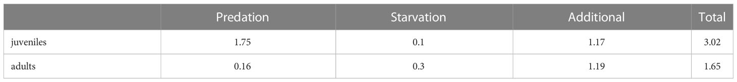
Table 1 Mortality rates (y^–1) of mesopelagic fish for different sources of mortality diagnosed by OSMOSE averaged after spin-up.

In an additional sensitivity experiment, we investigated the effects of OSMOSE’s trophic web on mesopelagic fish. For this case, all groups except the mesopelagic fish were forced to collapse by increasing their larval mortality by two to three orders of magnitude. As a result, mesopelagic fish was the only higher trophic level in the simulation. There were no other species preying on them and they fed exclusively on plankton. This simulation is denoted as “OSMOSE without trophic web”.

2.3 The mesopelagic fish model by A2019

A2019 proposed a steady-state flow analysis to estimate biomass of mesopelagic fish. Based on a set of linear equations and on steady state assumptions, this model differs in many ways from OSMOSE, among them the lack of differential equations and the linear dependence of fish biomass on primary production. We here outline the basic structure of this model, and refer the reader to the more detailed description and extensive sensitivity analysis by A2019. The model simulates a food web where organic matter produced by primary production can either be consumed by zooplankton in the epipelagic region or is exported as detritus to the deep water. The model by A2019 parameterizes three groups of zooplankton: epipelagic zooplankton which solely lives and feeds in the photic zone, migratory zooplankton which perform dial vertical migrations and detritivorous zooplankton that lives all the time in the deep water and feeds exclusively on sinking organic matter. These groups are consumed by carnivorous zooplankton, representing organisms such as chaetognaths, amphipods and jellyfish. Mesopelagic fish are at the top of the food chain consuming all zooplankton groups. The model assumes that one fraction of mesopelagic fish performs vertical migrations, hence feeding also on epipelagic zooplankton, and the rest remains permanently in the deep water. Metabolic losses are subtracted from the feeding flux. The resulting net growth of mesopelagic fish is then divided by a mortality rate to obtain the standing stock of mesopelagic fish. Given the linear dependency of fish biomass on (the inverse of) mortality rate, it is clear that the value of this parameter is of paramount importance, and we discuss the choices for this parameter value further down below.

The model by A2019 was designed to simulate meopelagic fish in the global ocean between 40° and 40°N. Therefore, it is reasonable to apply this model in the ETSP. To adapt the model specifically to the ETSP, we forced the model by A2019 with spatially resolved primary production extracted from the BioEBUS hindcast from 1990 to 2010 (see Section 4.1). We consider the mesopelagial as the vertical domain between 200 and 1000 m depth. To account for the restriction of this domain in regions shallower than 1000 m, we masked and scaled the primary production linearly for regions where the water depth is between 200 and 1000 m depth. For regions where the topography is shallower than 200 m, no primary production is extracted since we assume that no mesopelagic fish live in this region. Where the depth is 1000 m or deeper, we account for all integrated primary production. The resulting 2-dimensional output is used as spatially resolved forcing for the model by A2019.

OSMOSE and the model by A2019 are structurally different and there are two aspects that can be compared: the underlying forcing (as plankton or primary production) and the mortality. All other processes are set up in a completely different way. The additional mortality in OSMOSE is set to 1.19 y^–1 and, in addition to this, the mesopelagic fish are also subjected to predation and starvation mortality. In the model by A2019, the mortality is assumed to be much smaller and set to 0.67 y^–1, based on observational estimates of fish longevity. A2019 classified mortality as one of the most uncertain parameters in their model. Therefore, they carried out a sensitivity analysis adding +/- 75% to the parameter which resulted in a range of 0.17 to 1.17 y^–1. The upper boundary of this mortality range is close to the additional mortality value that we applied to OSMOSE (1.19 y^–1). However, the justification of the mortality in the model by A2019 does not account for processes such as starvation and predation explicitly. Since the mortality rate calculated by OSMOSE already accounts for the explicit impact of these processes, it might be a better estimate than the mortality by A2019. In addition, the model by A2019 does not account for different life stages of mesopelagic fish. We see in Table 1 that, in OSMOSE, the mortality of juveniles is almost twice as high as the mortality of adults, mostly due to the increased predation. To investigate the potential impact of accounting for the loss of juvenile fish (by mortality), we performed two sensitivity simulations: (i) applying the total mortality of adult mesopelagic fish as given by OSMOSE of 1.65 y^–1 to the model by A2019 and (ii) applying the total mortality of juvenile mesopelagic fish of 3.02 y^–1 to the model by A2019.

3 Results

The spatial distribution of the mesopelagic fish simulated with OSMOSE and with the model by A2019 using BioEBUS primary production is similar (Figure 1). The mesopelagic fish are absent in the coastal shallow water, which, for the model by A2019, was masked from the primary production input (Section 4.3), and their largest concentration is present off Peru. Independent of the choice of the mortality value, the model by A2019 produces a larger biomass than OSMOSE (Figure 1 top). Applying the larger mortality of 3.02 y^–1 to the model by A2019 (Figure 1 top middle), the resulting total biomass is about 26% larger than the biomass in OSMOSE, whereas applying the lower mortality of 1.65 y^–1 (Figure 1 top right) results in a total biomass that is about 130% larger than in OSMOSE (0.0208, 0.0262 and 0.0476 Gt WW of biomass estimated by OSMOSE, A2019 with high mortality and A2019 with low mortality respectively, Figure 1). The results indicate that the representation of different life stages of mesopelagic fish is likely to impact the resulting biomass. In our case, the comparatively large mortality of the juvenile fish in OSMOSE seems to play an important role and needs to be taken into account by the flux representations of the model by A2019. In the following we analyze the simulation with the higher mortality only (3.02 y^–1), which is closer to the output from OSMOSE.

FIGURE 1

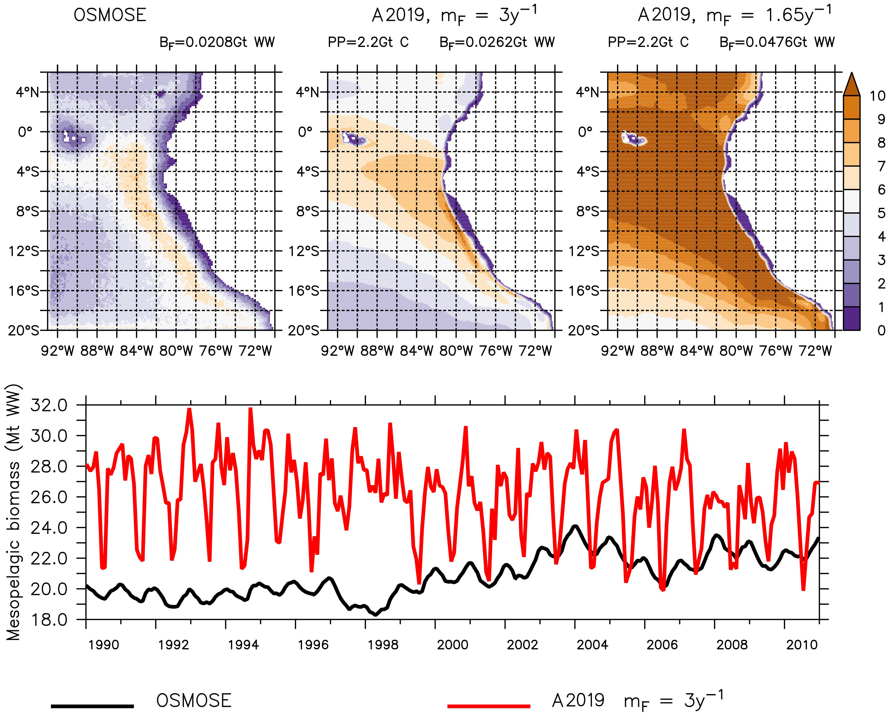
Figure 1 Mesopelagic fish simulated by OSMOSE (top-left and bottom-black) and the model by A2019 (top-middle, top-right and bottom-red), both models using input by CROCO–BioEBUS. The top row shows the averaged output in grams of wet weight per square meter (g WW m⁻²) from 1990 to 2010 and the bottom shows the total biomass over the domain for the same time period. The top row also gives the spatially integrated total primary production (PP), the total mesopelagic fish biomass (B^F) and the mortality rate applied to the model by A2019 (m^F; see Table 1).

The seasonal cycle in both higher trophic level models has the same frequency, but the amplitude of the mesopelagic fish biomass is much larger in the model by A2019 compared to the one in OSMOSE (Figure 1 bottom). In the model by A2019, mesopelagic fish biomass is a linear function of primary production, hence the anomaly of the interannual variability of the mesopelagic fish biomass in the model by A2019 is identical to the anomaly of the interannual variability of BioEBUS’ primary production (Figure 2). In contrast to that, we find that the amplitude of the seasonal cycle in OSMOSE is muted whereas the amplitude of its interannual variability is larger compared to the one in the model by A2019 and does not follow the same trend as the plankton input (Figure 2). In addition, the anomaly in mesopelagic fish biomass simulated by OSMOSE does not seem to follow the trend observed in BioEBUS’ plankton biomass. The decoupling is indicated by a weak cross correlation of maximal 0.197 (see Appendix).

FIGURE 2

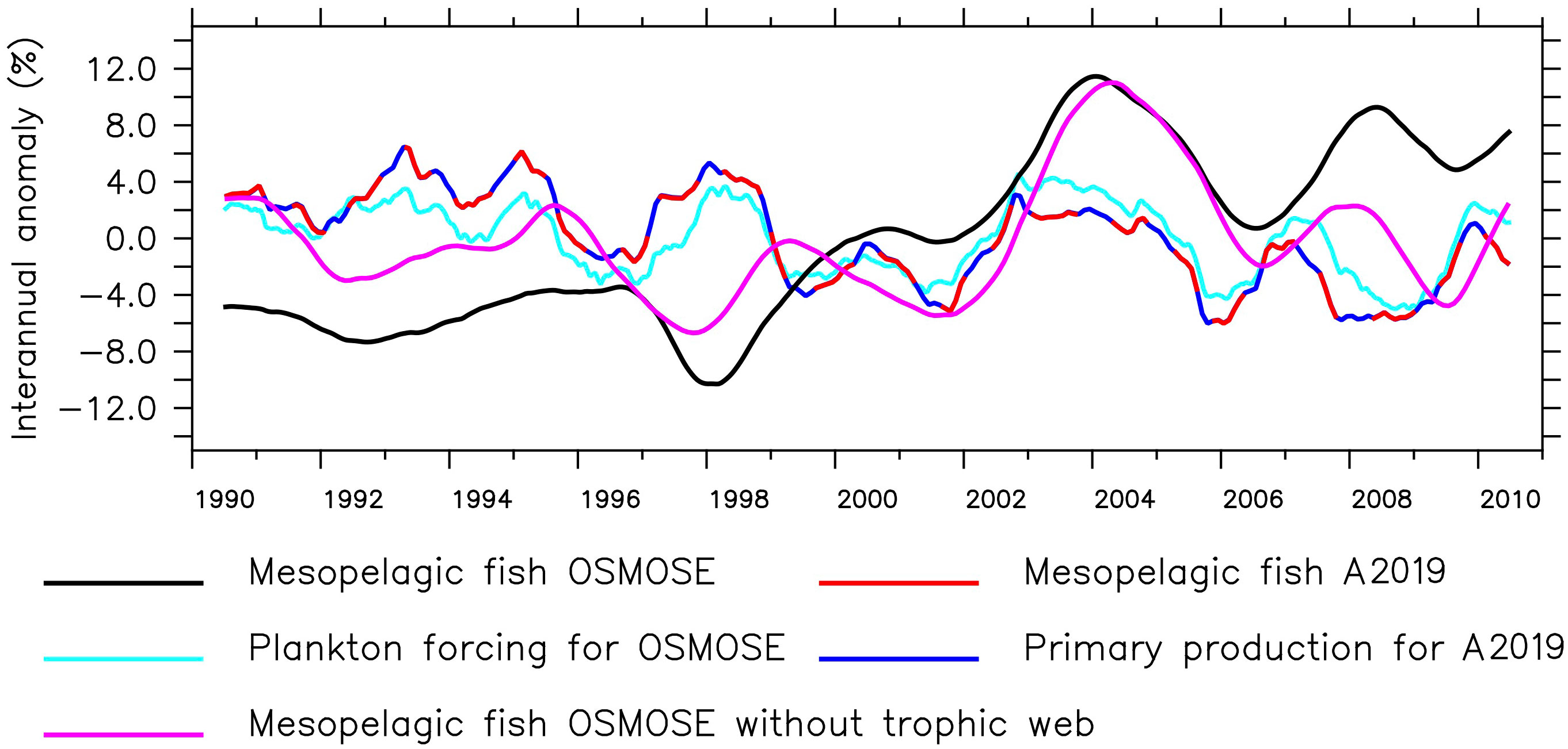
Figure 2 Anomaly of the 12-month running mean of total mesopelagic fish biomass calculated by OSMOSE and the model by A2019, primary production used as input for the model by A2019, total plankton biomass used to force OSMOSE and OSMOSE mesopelagic fish when all other fish groups were collapsed (see Section 2.2).

While the temporal variability in the model by A2019 is solely driven by the primary production, in OSMOSE it originates from the interplay of many other factors. These include the explicit life cycle of the fish, the trophic interactions with predators and different sources of prey, the spatial distribution of the fish and the variability in different sources of mortality. The main predator of mesopelagic fish in OSMOSE is the Humboldt squid. The main prey of mesopelagic fish are euphausiids and then large zooplankton. Removing all fish groups from the OSMOSE configuration except for the mesopelagics (Figure 2, pink line) resulted in a decrease in the amplitude of the interannual anomaly of mesopelagic fish biomass. In this simulation, there is a maximum cross correlation of 0.65 between the 12-month running means of plankton forcing and mesopelagic biomass with a lag of 8 months (see Appendix). The lag indicates that the fish biomass responds to changes in plankton forcing after about 8 months. This points to an impact of simulating a complex life cycle in OSMOSE, including egg production, by delaying the biomass response to plankton abundance. In summary, both the model by A2019 and OSMOSE show a similar seasonal cycle following the trend of the plankton and primary production. However, the interannual variability in OSMOSE is stronger and follows a different pattern even if mesopelagic fish are the only group present in this model.

4 Discussion

In our study, we observed a higher biomass in the model by A2019 than in OSMOSE of about 26 to 130%, depending on the mortality used. In general, mortality in numerical models is a highly uncertain parameter. As seen in this study, depending on the underlying assumptions, anticipate the mortality of juveniles or that of adult, the resulting biomass of mesopelagic fish can differ substantially.

OSMOSE model was calibrated to match observed biomasses of mesopelagic fish off Peru between 2000 and 2008 provided by the Instituto del Mar del Peru (IMARPE) as described in Hill Cruz et al. (2022). Nonetheless, acoustic estimates of mesopelagic fish are prone to high uncertainty (Marzloff et al., 2009; Davison et al., 2015a; Davison et al., 2015b). In addition, observations by IMARPE are done within the Exclusive Economic Zone of Peru (maximum distance to the coast of 100 to 200 nautical miles, see Castillo Valderrama and Gutiérrez Torero, 2001; Castillo Valderrama et al., 2004; Castillo Valderrama et al., 2009a; Castillo Valderrama et al., 2009b; Castillo Valderrama et al., 2009c). Castillo Valderrama et al. (1999) suggest that the abundance of Vinciguerria lucetia might be underestimated in a case where the transects were done closer to the shore since this is an oceanic species. Hence, the somewhat high mortality of mesopelagic fish could stem from the low bias of observations against which OSMOSE was calibrated.

Determining mortality rate $M$, and its sources, of fish species in the ocean is not straightforward. A2019 derived the value of $M=0.67$ y^–1 by calculating the inverse of a 1.5 year longevity ($t_{\max }$). While using longevity to estimate natural mortality is a convenient method when limited information is available, it might be an oversimplification and has been discouraged when more advanced methods are available (Kenchington, 2014). Often, longevity is determined from otoliths of caught fish (Takagi et al., 2006; Hosseini-Shekarabi et al., 2015). This reflects the age of the fish that survived until they were captured and provide information on how long a fish may live under certain circumstances, but does not distinguish between different processes such as predation, disease or starvation. There are a number of different methods to determine the natural mortality that involve longevity (see Kenchington, 2014; Then et al., 2014). The so called rule of thumb is also a function of longevity and estimates mortality as $M\approx 3/t_{\text{max}}$(Hewitt and Hoenig, 2005; Maunder and Wong, 2011). Applying this rule of thumb to mesopelagic fish, assuming a longevity of 1.5 years as in A2019, would result in a mortality of 2 y^–1, which is larger compared to the value of 0.67 y^–1 used in A2019. Then et al. (2014) derived a different relation between mortality and longevity based on information from more than 200 fish species: $M=4.899t_{max}^{-0.916}$ that yields a mortality of 3.38 y^–1 for our particular case. This is closer to our 3.02 y^–1 value estimated by OSMOSE for juvenile fish. Other approaches provide even higher values. For instance, the estimator by Hoenig (1983) for fish ($M=6.99t_{max}^{-1.22}$, see Kenchington, 2014) applied to mesopelagic fish results in a mortality of 4.26 y^–1. In summary, our results suggest that the mortality estimated by OSMOSE is within the range of mortality estimates obtained with other methods based on longevity. Therefore, mortality rates diagnosed from OSMOSE can support the parameterization of less complex food web models since its higher complexity includes explicit and dynamic sources of mortality including starvation and predation for different life stages of the fish.

Both OSMOSE and the model by A2019 offer advantages and disadvantages. The model by A2019 represents the mass transfer from nutrients over plankton to mesopelagic fish in a strainghtforward way. Its simplicity allows us to carry out many sensitivity experiments that address the effects of a changing biogeochemistry on fish.

The comprehensive parameter uncertainty analysis carried out by A2019 provided low and high boundaries for the integrated biomass estimates between 40°N and 40°S. Such an approach becomes more complicated with OSMOSE since running this individual-based model requires higher computational resources; also the model species may collapse under certain conditions (see Supplement to Hill Cruz et al., 2022). Therefore, for unconstrained regions, especially in the high seas, the model by A2019 can be used for providing first estimates of potential mesopelagic fish biomass. Nevertheless, the model by A2019 does not explicitly simulate life cycles or a trophic web but only represents the (linear) biomass transfer from primary production to mesopelagic fish as a steady state. This might be an oversimplification for a highly dynamic region such as the ETSP where environmental variability has been seen to have strong impacts on small pelagic fish (Chavez et al., 2003; Alheit and Niquen, 2004). A dynamic model is necessary to study potential responses of this type in mesopelagic fish and to estimate a population growth rate and recruitment based on life traits.

The individual-based model OSMOSE represents the whole life cycle of several fish and macroinvertebrate species. Since this is a dynamic model, it is a good alternative for representing non-linear changes in fish populations triggered by different pressures such as environmental variability. Our results show that the non-linearity affects how mesopelagic fish respond to variability in their food, which is produced by environmental changes. As a multispecies model, OSMOSE is also useful for exploring fishing strategies in an ecosystem-based fisheries management context (Briton et al., 2019; Fu et al., 2019; Guo et al., 2019; Fu et al., 2020). There is growing evidence of the importance of mesopelagic fish in deep water food chains (Mann, 1984; Davison et al., 2015a; Saunders et al., 2019). In our study, the main predator of mesopelagic fish is the Humboldt squid (see Appendix). This is a species of economic importance (Gilly et al., 2013) that feeds mainly on mesopelagic fish (Markaida and Sosa-Nishizaki, 2003). Therefore, any prospect on the exploitation of mesopelagic fish in the ETSP should consider the potential impacts on this species. Likewise, changes in the exploitation on the Humboldt squid should consider potential cascading effects on the mesopelagic fish and lower trophic levels. Furthermore, while the spatial distribution offshore in the model by A2019 was fully dependent on the primary production, in OSMOSE the distribution of fish schools is forced by habitat niche models. These maps vary in time and can be used to simulate horizontal migrations (see Grüss et al., 2014; Oliveros-Ramos, 2014) allowing for further refinement in the distribution of fish when this information is available. Nevertheless, our results show a similar spatial pattern in both OSMOSE and the model by A2019. This indicates that the food source has a strong impact on the distribution of mesopelagic fish. Hence, the approach used in the model by A2019 can provide a first idea of the distribution of mesopelagic fish where observations and habitat niche models are not available, for instance in a global setting.

Both OSMOSE and the model by A2019 lack a vertical dimension of fish distribution, but parameterize its effect on the trophic web. In the case of OSMOSE, this is done through a predatory accessibility matrix which constrains which fish groups can feed on others based on their hypothetical position in the water column. The model by A2019 goes a step further by also parameterizing vertical migrations of mesopelagic fish. It assumes in its trophic chain that migrant fish feed on epipelagic zooplankton for half of the day and on migrating zooplankton all day [A2019]. Vertical migrations are especially important in the context of mesopelagic fish due to their role in the active transport of organic matter to the deep ocean (Davison et al., 2013; Belcher et al., 2019; Hernández-León et al., 2019) and its implications for carbon capture, oxygen loss and nutrient cycles. However, vertical migrations are only implicitly represented in the model by A2019. A full coupling of the model by A2019 to the biogeochemical model would be necessary to capture the impact of vertical migrations on biogeochemical cycles.

5 Conclusions

Depending on the mortality rates applied, the biomass estimated by the model by A2019 was more or less (26% with high mortality and 130% with low mortality) higher than in OSMOSE. In both cases, the mortalities calculated by OSMOSE were larger than the original mortality estimated as the inverse of longevity by A2019. Although OSMOSE has been calibrated to match the limited amount of observations available for the coastal region of the ETSP, uncertainties are large with respect to the open ocean where mesopelagic fish are abundant. To reduce this uncertainty, more reliable estimates of mesopelagic fish biomass in the open ocean would be beneficial. OSMOSE exhibits a weaker seasonal cycle but a stronger interannual variability. On the contrary, the model by A2019 follows the same temporal pattern as the primary production forcing due to its linear nature. Looking ahead, both models have strengths and disadvantages. OSMOSE provides a richer representation of the life cycle and trophic interactions of the fish community. This is crucial for studies steered towards implementations of fisheries management. The strength of the model by A2019 lies in the direct, computationally efficient link between the biogeochemistry and the fish representation, which is useful for understanding potential boundaries for the available biomass of mesopelagic fish given certain biogeochemical conditions. The most comprehensive representation of the ecosystem could combine the strengths of both models. Being the most simple and computationally efficient approach, the model by A2019 could provide a first estimate for regions where data are limited, such as in the global ocean and the high seas. OSMOSE simulates a more comprehensive food web and is the preferred approach when observational data are available to calibrate the model. With its more detailed resolution of food web and ecological processes, it can also aid the validation of parameters in simpler models that do not have a direct observational counterpart such as mortality. In addition, model results can be assessed against many other quantities such as stomach content, trophic level, size structure and catches to provide a more accurate representation of the ecosystem.

Data availability statement

The raw data supporting the conclusions of this article will be made available by the authors, without undue reservation.

Author contributions

MH and IK designed the experiments. IK set up the model by A2019. MH set up OSMOSE, carried out the simulations with both fish models coupled to the physical–biogeochemical model and analyzed the data. All authors discussed the results and wrote the manuscript. All authors contributed to the article and approved the submitted version.

Funding

This study received financial support by the Bundesministerium für Bildung und Forschung (BMBF) through the projects Coastal Upwelling System in a Changing Ocean CUSCO (03F0813 A), Humboldt-Tipping (01LC1823B) and CO2Meso (03F0876A). Model simulations were carried out using the facilities of the Norddeutscher Verbund zur Förderung des Hoch- und Höchstleistungsrechnens – HLRN

Acknowledgments

We thank the two reviewers for their valuable comments to improve the manuscript and we thank Tronje Kemena for the helpful discussions and his suggestion of using cross correlations to improve our analysis.

Conflict of interest

The authors declare that the research was conducted in the absence of any commercial or financial relationships that could be construed as a potential conflict of interest.

Publisher’s note

All claims expressed in this article are solely those of the authors and do not necessarily represent those of their affiliated organizations, or those of the publisher, the editors and the reviewers. Any product that may be evaluated in this article, or claim that may be made by its manufacturer, is not guaranteed or endorsed by the publisher.

References

Ainsworth C. H., Schirripa M. J., Morzaria-Luna H. N. (2015). An Atlantis ecosystem model for the Gulf of Mexico supporting integrated ecosystem assessment (Florida, USA: U.S. DEPARTMENT OF COMMERCE National Oceanic and Atmospheric Administration National Marine Fisheries Service Southeast Fisheries Science). doi: 10.7289/V5X63JVH

CrossRef Full Text | Google Scholar

Alheit J., Niquen M. (2004). Regime shifts in the Humboldt Current ecosystem. Prog. Oceanogr. 60, 201–222. doi: 10.1016/j.pocean.2004.02.006

CrossRef Full Text | Google Scholar

Anderson T. R., Martin A. P., Lampitt R. S., Trueman C. N., Henson S. A., Mayor D. J. (2019). Quantifying carbon fluxes from primary production to mesopelagic fish using a simple food web model. ICES J. Mar. Sci. 76, 690–701. doi: 10.1093/icesjms/fsx234

CrossRef Full Text | Google Scholar

Atlas R., Hoffman R. N., Bloom S. C., Jusem J. C., Ardizzone J. (1996). A Multiyear Global Surface Wind Velocity Dataset Using SSM/I Wind Observations. Bull. Am. Meteorol. Soc. 77, 869–882. doi: 10.1175/1520-0477(1996)077<0869:AMGSWV>2.0.CO;2

CrossRef Full Text | Google Scholar

Aumont O., Maury O., Lefort S., Bopp L. (2018). Evaluating the potential impacts of the diurnal vertical migration by marine organisms on marine biogeochemistry. Global Biogeochem. Cycles 32, 1622–1643. doi: 10.1029/2018GB005886

CrossRef Full Text | Google Scholar

Bănaru D., Diaz F., Verley P., Campbell R., Navarro J., Yohia C., et al. (2019). Implementation of an end-to-end model of the Gulf of Lions ecosystem (NW Mediterranean Sea). I. Parameterization, calibration and evaluation. Ecol. Model. 401, 1–19. doi: 10.1016/j.ecolmodel.2019.03.005

CrossRef Full Text | Google Scholar

Belcher A., Saunders R., Tarling G. (2019). Respiration rates and active carbon flux of mesopelagic fishes (Family Myctophidae) in the Scotia Sea, Southern Ocean. Mar. Ecol. Prog. Ser. 610, 149–162. doi: 10.3354/meps12861

CrossRef Full Text | Google Scholar

Bertrand A., Chaigneau A., Peraltilla S., Ledesma J., Graco M., Monetti F., et al. (2011). A Fundamental Property Regulating Pelagic Ecosystem Structure in the Coastal Southeastern Tropical Pacific. PloS One 6, 1–8. doi: 10.1371/journal.pone.0029558

CrossRef Full Text | Google Scholar

Bianchi D., Carozza D. A., Galbraith E. D., Guiet J., DeVries T. (2021). Estimating global biomass and biogeochemical cycling of marine fish with and without fishing. Sci. Adv. 7, eabd7554. doi: 10.1126/sciadv.abd7554

PubMed Abstract | CrossRef Full Text | Google Scholar

Briton F., Shannon L., Barrier N., Verley P., Shin Y.-J. (2019). Reference levels of ecosystem indicators at multispecies maximum sustainable yield. ICES J. Mar. Sci. 76, 2070–2081. doi: 10.1093/icesjms/fsz104

CrossRef Full Text | Google Scholar

Carozza D. A., Bianchi D., Galbraith E. D. (2016). The ecological module of BOATS-1.0: a bioenergetically constrained model of marine upper trophic levels suitable for studies of fisheries and ocean biogeochemistry. Geoscientific Model. Dev. 9, 1545–1565. doi: 10.5194/gmd-9-1545-2016

CrossRef Full Text | Google Scholar

Carton J. A., Chepurin G. A., Chen L. (2018). SODA3: A new ocean climate reanalysis. J. Climate 31, 6967–6983. doi: 10.1175/JCLI-D-18-0149.1

CrossRef Full Text | Google Scholar

Castillo Valderrama R., Gutiérrez Torero M. (2001). Biomasas de las once especies pesqueras más abundancia en el mar peruano durante el verano 2000 (Callao, Peru: Instituto del Mar del Perú IMARPE).

Google Scholar

Castillo Valderrama R., Gutiérrez Torero M., Herrera Almirón N. (2004). Biomasa de siete especies pelágicas abundantes en el mar peruano durante el verano austral 2001 (Callao, Peru: Informe IMARPE 1, Instituto del Mar del Perú).

Google Scholar

Castillo Valderrama R., Gutiérrez Torero M., Peraltilla Neyra S., Escudero Herrera L. (2009a). Distribución y biomasa de los principales recursos pelágicos del mar peruano. verano 2006 (Callao, Peru: Informe IMARPE 3-4, Instituto del Mar del Perú).

Google Scholar

Castillo Valderrama R., Gutiérrez Torero M., Peraltilla Neyra S., Herrera Almirón N. (1998). Biomasa de recursos pesqueros a finales del invierno 1998. crucero BIC Humboldt y BIC Jose Olaya Balandra 9808-09, de Paita a Tacna (Callao, Peru: Informe IMARPE 141, Instituto del Mar del Perú).

Google Scholar

Castillo Valderrama R., Gutiérrez Torero M., Peraltilla Neyra S., Herrera Almirón N. (1999). Biomasas de las principales especies recursos pesqueros durante el verano 1999. crucero BIC Jose Olaya Balandra 9902-03, de Tumbes a Tacna (Callao, Peru: Informe IMARPE 147, Instituto del Mar del Perú).

Google Scholar

Castillo Valderrama R., Gutiérrez Torero M., Segura Zamudio M., Peraltilla Neyra S. (2009b). Distribución y biomasa de algunos recursos pelágicos peruanos en verano 2004 (Callao, Peru: Informe IMARPE 1-2, Instituto del Mar del Perú).

Google Scholar

Castillo Valderrama R., Segura Zamudio M., Gutiérrez Torero M., Ganoza Chozo F., Peraltilla Neyra S. (2009c). Distribución y biomasa de algunos recursos pelágicos peruanos. verano 2003 (Callao, Peru: Informe IMARPE 1-2, Instituto del Mar del Perú).

Google Scholar

Chavez F. P., Bertrand A., Guevara-Carrasco R., Soler P., Csirke J. (2008). The northern Humboldt Current System: Brief history, present status and a view towards the future. Prog. Oceanogr. 79, 95–105. doi: 10.1016/j.pocean.2008.10.012

CrossRef Full Text | Google Scholar

Chavez F. P., Ryan J., Lluch-Cota S. E., Ñiquen M. (2003). From Anchovies to Sardines and Back: Multidecadal Change in the Pacific Ocean. Science 299, 217–221. doi: 10.1126/science.1075880

PubMed Abstract | CrossRef Full Text | Google Scholar

Colléter M., Valls A., Guitton J., Gascuel D., Pauly D., Christensen V. (2015). Global overview of the applications of the Ecopath with Ecosim modeling approach using the EcoBase models repository. Ecol. Model. 302, 42–53. doi: 10.1016/j.ecolmodel.2015.01.025

CrossRef Full Text | Google Scholar

Cornejo Urbina R., Koppelmann R. (2006). Distribution patterns of mesopelagic fishes with special reference to Vinciguerria lucetia Garman 1899 (Phosichthyidae: Pisces) in the Humboldt Current Region off Peru. Mar. Biol. 149, 1519–1537. doi: 10.1007/s00227-006-0319-z

CrossRef Full Text | Google Scholar

Davison P., Checkley D., Koslow J., Barlow J. (2013). Carbon export mediated by mesopelagic fishes in the northeast Pacific Ocean. Prog. Oceanogr. 116, 14–30. doi: 10.1016/j.pocean.2013.05.013

CrossRef Full Text | Google Scholar

Davison P. C., Koslow J. A., Kloser R. J. (2015b). Acoustic biomass estimation of mesopelagic fish: backscattering from individuals, populations, and communities. ICES J. Mar. Sci. 72, 1413–1424. doi: 10.1093/icesjms/fsv023

CrossRef Full Text | Google Scholar

Davison P., Lara-Lopez A., Anthony Koslow J. (2015a). Mesopelagic fish biomass in the southern California current ecosystem. Deep Sea Res. Part II: Topical Stud. Oceanogr. 112, 129–142. doi: 10.1016/j.dsr2.2014.10.007

CrossRef Full Text | Google Scholar

Duffy D. C. (1983). Environmental uncertainty and commercial fishing: Effects on Peruvian guano birds. Biol. Conserv. 26, 227–238. doi: 10.1016/0006-3207(83)90075-7

CrossRef Full Text | Google Scholar

Fu C., Xu Y., Grüss A., Bundy A., Shannon L., Heymans J. J., et al. (2019). Responses of ecological indicators to fishing pressure under environmental change: exploring non-linearity and thresholds. ICES J. Mar. Sci. 77, 1516–1531. doi: 10.1093/icesjms/fsz182

CrossRef Full Text | Google Scholar

Fu C., Xu Y., Guo C., Olsen N., Grüss A., Liu H., et al. (2020). The cumulative effects of fishing, plankton productivity, and marine mammal consumption in a marine ecosystem. Front. Mar. Sci. 7. doi: 10.3389/fmars.2020.565699

CrossRef Full Text | Google Scholar

Fulton E. A. (2010). Approaches to end-to-end ecosystem models. J. Mar. Syst. 81, 171–183. doi: 10.1016/j.jmarsys.2009.12.012

CrossRef Full Text | Google Scholar

Getzlaff J., Oschlies A. (2017). Pilot study on potential impacts of fisheries-induced changes in zooplankton mortality on marine biogeochemistry. Global Biogeochem. Cycles 31, 1656–1673. doi: 10.1002/2017GB005721

CrossRef Full Text | Google Scholar

Gilly W. F., Beman J. M., Litvin S. Y., Robison B. H. (2013). Oceanographic and biological effects of shoaling of the oxygen minimum zone. Annu. Rev. Mar. Sci. 5, 393–420. doi: 10.1146/annurev-marine-120710-100849

CrossRef Full Text | Google Scholar

Gjøsæter J., Kawaguchi K. (1980). A review of the world resources of mesopelagic fish. FAO fisheries technical paper 193. Food Agric. Organ.

Google Scholar

Grüss A., Drexler M., Ainsworth C. H. (2014). Using delta generalized additive models to produce distribution maps for spatially explicit ecosystem models. Fisheries Res. 159, 11–24. doi: 10.1016/j.fishres.2014.05.005

CrossRef Full Text | Google Scholar

Guo C., Fu C., Olsen N., Xu Y., Grüss A., Liu H., et al. (2019). Incorporating environmental forcing in developing ecosystem-based fisheries management strategies. ICES J. Mar. Sci. 77, 500–514. doi: 10.1093/icesjms/fsz246

CrossRef Full Text | Google Scholar

Gutknecht E., Dadou I., Le Vu B., Cambon G., Sudre J., Garçon V., et al. (2013). Coupled physical/biogeochemical modeling including O2-dependent processes in the Eastern Boundary Upwelling Systems: application in the Benguela. Biogeosciences 10, 3559–3591. doi: 10.5194/bg-10-3559-2013

CrossRef Full Text | Google Scholar

Halouani G., Lasram F., Shin Y.-J., Velez L., Verley P., Hattab T., et al. (2016). Modelling food web structure using an end-to-end approach in the coastal ecosystem of the Gulf of Gabes (Tunisia). Ecol. Model. 339, 45–57. doi: 10.1016/j.ecolmodel.2016.08.008

CrossRef Full Text | Google Scholar

Herling C., Culik B. M., Hennicke J. C. (2005). Diet of the Humboldt penguin (Spheniscus humboldti) in northern and southern Chile. Mar. Biol. 147, 13–25. doi: 10.1007/s00227-004-1547-8

CrossRef Full Text | Google Scholar

Hernández-León S., Olivar M. P., Fernández de Puelles M. L., Bode A., Castellón A., López-Pérez C., et al. (2019). Zooplankton and Micronekton Active Flux Across the Tropical and Subtropical Atlantic Ocean. Front. Mar. Sci. 6. doi: 10.3389/fmars.2019.00535

CrossRef Full Text | Google Scholar

Hewitt D. A., Hoenig J. M. (2005). Comparison of two approaches for estimating natural mortality based on longevity. Fishery Bull. 103, 433–437.

Google Scholar

Hill Cruz M., Frenger I., Getzlaff J., Kriest I., Xue T., Shin Y.-J. (2022). Understanding the drivers of fish variability in an end-to-end model of the Northern Humboldt Current System. Ecol. Model. 472, 110097. doi: 10.1016/j.ecolmodel.2022.110097

CrossRef Full Text | Google Scholar

Hoenig J. M. (1983). Empirical use of longevity data to estimate mortality rates. Fishery Bull. 81, 898–903.

Google Scholar

Hosseini-Shekarabi S. P., Valinassab T., Bystydzieńska Z., Linkowski T. (2015). Age and growth of Benthosema Pterotum (Alcock 1890) (Myctophidae) in the Oman Sea. J. Appl. Ichthyol.0 31, 51–56. doi: 10.1111/jai.12620

CrossRef Full Text | Google Scholar

Irigoien X., Klevjer T. A., Røstad A., Martinez U., Boyra G., Acuña J. L., et al. (2014). Large mesopelagic fishes biomass and trophic efficiency in the open ocean. Nat. Commun. 5, 3271. doi: 10.1038/ncomms4271

PubMed Abstract | CrossRef Full Text | Google Scholar

José Y. S., Stramma L., Schmidtko S., Oschlies A. (2019). ENSO-driven fluctuations in oxygen supply and vertical extent of oxygen-poor waters in the oxygen minimum zone of the Eastern Tropical South Pacific. Biogeosci. Discussions 2019, 1–20. doi: 10.5194/bg-2019-155

CrossRef Full Text | Google Scholar

Karstensen J., Stramma L., Visbeck M. (2008). Oxygen minimum zones in the eastern tropical Atlantic and Pacific oceans. Prog. Oceanogr. 77, 331–350. doi: 10.1016/j.pocean.2007.05.009

CrossRef Full Text | Google Scholar

Kenchington T. J. (2014). Natural mortality estimators for information-limited fisheries. Fish Fisheries 15, 533–562. doi: 10.1111/faf.12027

CrossRef Full Text | Google Scholar

Köster F. W., Möllmann C. (2000). Trophodynamic control by clupeid predators on recruitment success in Baltic cod? ICES J. Mar. Sci. 57, 310–323. doi: 10.1006/jmsc.1999.0528

CrossRef Full Text | Google Scholar

Mann K. H. (1984). Fish production in open ocean ecosystems (Boston, MA: Springer US), 435–458. doi: 10.1007/978-1-4757-0387-0

CrossRef Full Text | Google Scholar

Markaida U., Sosa-Nishizaki O. (2003). Food and feeding habits of jumbo squid Dosidicus gigas (Cephalopoda: Ommastrephidae) from the Gulf of California, Mexico. J. Mar. Biol. Assoc. United Kingdom 83, 507—522. doi: 10.1017/S0025315403007434h

CrossRef Full Text | Google Scholar

Martin A., Boyd P., Buesseler K., Cetinic I., Claustre H., Giering S., et al. (2020). The oceans’ twilight zone must be studied now, before it is too late. Nature 580, 26–28. doi: 10.1038/d41586-020-00915-7

PubMed Abstract | CrossRef Full Text | Google Scholar

Marzloff M., Shin Y.-J., Tam J., Travers M., Bertrand A. (2009). Trophic structure of the Peruvian marine ecosystem in 2000-2006: Insights on the effects of management scenarios for the hake fishery using the IBM trophic model Osmose. J. Mar. Syst. 75, 290–304. doi: 10.1016/j.jmarsys.2008.10.009

CrossRef Full Text | Google Scholar

Maunder M. N., Wong R. A. (2011). Approaches for estimating natural mortality: Application to summer flounder (Paralichthys dentatus) in the U.S. mid-Atlantic. Fisheries Res. 111, 92–99. doi: 10.1016/j.fishres.2011.06.016

CrossRef Full Text | Google Scholar

Megrey B. A., Rose K. A., Klumb R. A., Hay D. E., Werner F. E., Eslinger D. L., et al. (2007). A bioenergetics-based population dynamics model of Pacific herring (Clupea harengus pallasi) coupled to a lower trophic level nutrient–phytoplankton–zooplankton model: Description, calibration, and sensitivity analysis. Ecol. Model. 202, 144–164. doi: 10.1016/j.ecolmodel.2006.08.020

CrossRef Full Text | Google Scholar

Oliveros-Ramos R. (2014). End–to–end modelling for an ecosystem approach to fisheries in the Northern Humboldt Current Ecosystem (France: University of Montpellier). Ph.D. thesis.

Google Scholar

Pauly D., Christensen V., Walters C. (2000). Ecopath, Ecosim, and Ecospace as tools for evaluating ecosystem impact of fisheries. ICES J. Mar. Sci. 57, 697–706. doi: 10.1006/jmsc.2000.0726

CrossRef Full Text | Google Scholar

Péron G., François Mittaine J., Le Gallic B. (2010). Where do fishmeal and fish oil products come from? An analysis of the conversion ratios in the global fishmeal industry. Mar. Policy 34, 815–820. doi: 10.1016/j.marpol.2010.01.027

CrossRef Full Text | Google Scholar

Petrik C. M., Stock C. A., Andersen K. H., van Denderen P. D., Watson J. R. (2019). Bottom-up drivers of global patterns of demersal, forage, and pelagic fishes. Prog. Oceanogr. 176, 102124. doi: 10.1016/j.pocean.2019.102124

CrossRef Full Text | Google Scholar

Prosekov A. Y., Ivanova S. A. (2018). Food security: The challenge of the present. Geoforum 91, 73–77. doi: 10.1016/j.geoforum.2018.02.030

CrossRef Full Text | Google Scholar

Ridgway K., Dunn J., Wilkin J. (2002). Ocean Interpolation by Four-Dimensional Weighted Least Squares—Application to the Waters around Australasia. J. atmospheric oceanic Technol. 19, 1357–1375. doi: 10.1175/1520-0426(2002)019<1357:OIBFDW>2.0.CO;2

CrossRef Full Text | Google Scholar

Rose K. A., Fiechter J., Curchitser E. N., Hedstrom K., Bernal M., Creekmore S., et al. (2015). Demonstration of a fully-coupled end-to-end model for small pelagic fish using sardine and anchovy in the California Current. Prog. Oceanogr. 138, 348–380. doi: 10.1016/j.pocean.2015.01.012

CrossRef Full Text | Google Scholar

Saha S., Moorthi S., Pan H.-L., Wu X., Wang J., Nadiga S., et al. (2010). The NCEP Climate Forecast System Reanalysis. Bull. Am. Meteorol. Soc. 91, 1015–1058. doi: 10.1175/2010BAMS3001.1

CrossRef Full Text | Google Scholar

Salvatteci R., Schneider R. R., Galbraith E., Field D., Blanz T., Bauersachs T., et al. (2022). Smaller fish species in a warm and oxygen-poor Humboldt Current system. Science 375, 101–104. doi: 10.1126/science.abj0270

PubMed Abstract | CrossRef Full Text | Google Scholar

Saunders R. A., Hill S. L., Tarling G. A., Murphy E. J. (2019). Myctophid Fish (Family Myctophidae) Are Central Consumers in the Food Web of the Scotia Sea (Southern Ocean). Front. Mar. Sci. 6. doi: 10.3389/fmars.2019.00530

CrossRef Full Text | Google Scholar

Shchepetkin A. F., McWilliams J. C. (2005). The regional oceanic modeling system Myctophid Fish (Family Myctophidae) Are Central Consumers in the Food Web of the Scotia Sea (Southern Ocean): a split-explicit, free-surface, topography-following-coordinate oceanic model. Ocean Model. 9, 347–404. doi: 10.1016/j.ocemod.2004.08.002

CrossRef Full Text | Google Scholar

Shepherd C. J., Jackson A. J. (2013). Global fishmeal and fish-oil supply: inputs, outputs and marketsa. J. Fish Biol. 83, 1046–1066. doi: 10.1111/jfb.12224

PubMed Abstract | CrossRef Full Text | Google Scholar

Shin Y.-J., Cury P. (2001). Exploring fish community dynamics through size-dependent trophic interactions using a spatialized individual-based model. Aquat. Living Resour. 14, 65–80. doi: 10.1016/S0990-7440(01)01106-8

CrossRef Full Text | Google Scholar

Shin Y.-J., Cury P. (2004). Using an individual-based model of fish assemblages to study the response of size spectra to changes in fishing. Can. J. Fisheries Aquat. Sci. 61, 414–431. doi: 10.1139/f03-154

CrossRef Full Text | Google Scholar

St. John M. A., Borja A., Chust G., Heath M., Grigorov I., Mariani P., et al. (2016). A dark hole in our understanding of marine ecosystems and their services: Perspectives from the mesopelagic community. Front. Mar. Sci. 3. doi: 10.3389/fmars.2016.00031

CrossRef Full Text | Google Scholar

Swartzman G., Bertrand A., Gutiérrez M., Bertrand S., Vasquez L. (2008). The relationship of anchovy and sardine to water masses in the Peruvian Humboldt Current System from 1983 to 2005. Prog. Oceanogr. 79, 228–237. doi: 10.1016/j.pocean.2008.10.021

CrossRef Full Text | Google Scholar

Takagi K., Yatsu A., Moku M., Sassa C. (2006). Age and growth of lanternfishes, Symbolophorus californiensis and Ceratoscopelus warmingii (Myctophidae), in the Kuroshio–Oyashio Transition Zone. Ichthyological Res. 53, 281–289. doi: 10.1007/s10228-006-0346-2

CrossRef Full Text | Google Scholar

Tam J., Taylor M. H., Blaskovic V., Espinoza P., Michael Ballón R., Díaz E., et al. (2008). Trophic modeling of the Northern Humboldt Current Ecosystem, Part I: Comparing trophic linkages under La Niña and El Niño conditions. Prog. Oceanogr. 79, 352–365. doi: 10.1016/j.pocean.2008.10.007

CrossRef Full Text | Google Scholar

Tarazona J., Arntz W. (2001). The Peruvian coastal upwelling system (Berlin, Heidelberg: Springer Berlin Heidelberg), 229–244. doi: 10.1007/978-3-662-04482-7

CrossRef Full Text | Google Scholar

Then A. Y., Hoenig J. M., Hall N. G., Hewitt D. A. (2014). Evaluating the predictive performance of empirical estimators of natural mortality rate using information on over 200 fish species. ICES J. Mar. Sci. 72, 82–92. doi: 10.1093/icesjms/fsx199

CrossRef Full Text | Google Scholar

Tittensor D. P., Eddy T. D., Lotze H. K., Galbraith E. D., Cheung W., Barange M., et al. (2018). A protocol for the intercomparison of marine fishery and ecosystem models: Fish-MIP v1. 0. Geoscientific Model. Dev. 11, 1421–1442. doi: 10.5194/gmd-11-1421-2018

CrossRef Full Text | Google Scholar

Tittensor D. P., Novaglio C., Harrison C. S., Heneghan R. F., Barrier N., Bianchi D., et al. (2021). Next-generation ensemble projections reveal higher climate risks for marine ecosystems. Nat. Climate Change 11, 973–981. doi: 10.1038/s41558-021-01173-9

CrossRef Full Text | Google Scholar

Travers M., Shin Y.-J., Jennings S., Machu E., Huggett J., Field J., et al. (2009). Two-way coupling versus one-way forcing of plankton and fish models to predict ecosystem changes in the Benguela. Ecol. Model. 220, 3089–3099. doi: 10.1016/j.ecolmodel.2009.08.016

CrossRef Full Text | Google Scholar

Travers-Trolet M., Shin Y., Field J. (2014a). An end-to-end coupled model ROMS–N2P2Z2D2–OSMOSE of the southern Benguela foodweb: parameterisation, calibration and pattern-oriented validation. Afr. J. Mar. Sci. 36, 11–29. doi: 10.2989/1814232X.2014.883326

CrossRef Full Text | Google Scholar

Travers-Trolet M., Shin Y.-J., Shannon L. J., Moloney C. L., Field J. G. (2014b). Combined Fishing and Climate Forcing in the Southern Benguela Upwelling Ecosystem: An End-to-End Modelling Approach Reveals Dampened Effects. PloS One 9, e94286. doi: 10.1371/journal.pone.0094286

PubMed Abstract | CrossRef Full Text | Google Scholar

Watson J. R., Stock C. A., Sarmiento J. L. (2015). Exploring the role of movement in determining the global distribution of marine biomass using a coupled hydrodynamic – Size-based ecosystem model. Prog. Oceanogr. 138, 521–532. doi: 10.1016/j.pocean.2014.09.001

CrossRef Full Text | Google Scholar

Xue T., Frenger I., Prowe A., José Y. S., Oschlies A. (2022). Mixed layer depth dominates over upwelling in regulating the seasonality of ecosystem functioning in the Peruvian upwelling system. Biogeosciences 19, 455–475. doi: 10.5194/bg-19-455-2022

CrossRef Full Text | Google Scholar

Appendix

Figure A1 shows the position of mesopelagic fish in the modelled trophic web. The main prey of mesopelagic fish is euphausiids followed by plankton and their main predator is the Humboldt squid.

FIGURE A1

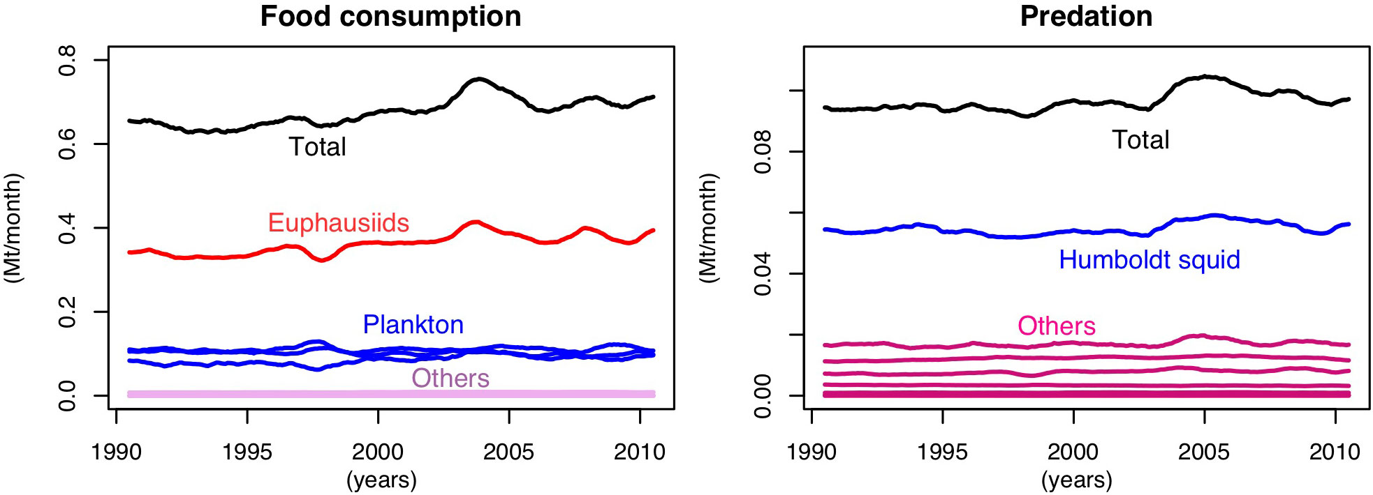
FIGURE A1 Monthly consumption by (left) and of (right) mesopelagic fish.

Figure A2 shows a higher absolute cross correlation in the OSMOSE simulation that only has mesopelagic fish, between these fish and the plankton forcing, than in the simulation that includes the whole food web (see Section 2.2).

FIGURE A2

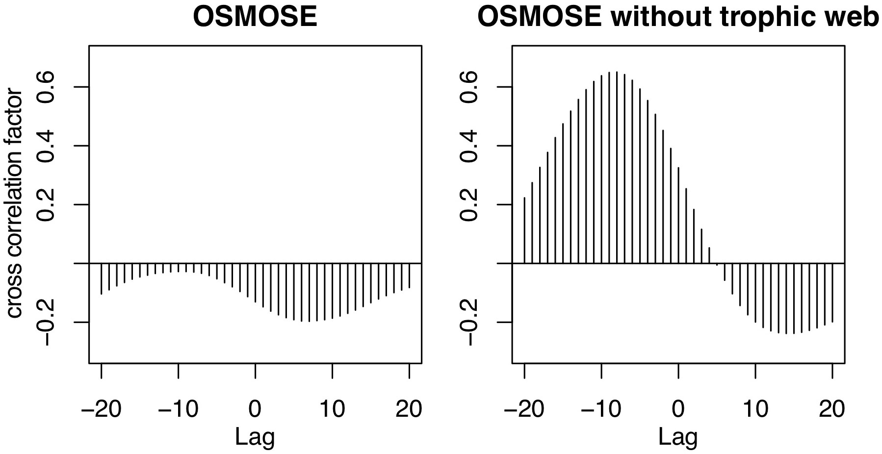
FIGURE A2 Cross correlation between the yearly running means of plankton forcing and mesopelagic fish biomass in OSMOSE simulations with monthly time-steps.