Atmospheric CO2 emissions and ocean acidification from bottom-trawling

1 Introduction

Marine sediments are thought to be the ultimate long-term carbon store; once buried below the active layer, organic carbon can remain unmineralized for millennia to eons (Burdige, 2007; LaRowe et al., 2020). However, disturbances to the seabed by human activities threaten the permanency of this marine carbon (Levin et al., 2020; Paradis et al., 2021). In the case of bottom trawling, heavy fishing gear that is dragged across the seafloor mixes and resuspends sediments, exposing 0.16-0.40 Pg C yr^-1 of previously buried organic carbon to potential microbial degradation (Sala et al., 2021). However, the ultimate fate of this disturbed organic carbon stock is as yet unquantified, hampering our understanding of the effects that bottom trawling has on the global carbon cycle and the potential implications for climate policies.

The protection of organic carbon stored in marine sediments, plants, and animals has been identified as a powerful tool for tackling climate change (Hoegh-Guldberg et al., 2019). However, the uptake of ocean-based climate solutions has been slow due to prevailing climate policies and carbon markets that only recognize mitigation activities with measurable impacts on atmospheric emissions. The challenge with identifying ocean-based solutions under those current paradigms lies in the complexity of quantifying atmospheric emissions generated by anthropogenic activities that occur below the ocean’s surface (Luisetti et al., 2020). Therefore, research addressing this challenge is crucial for discovering new opportunities that can harness the full potential of the ocean in contributing to mitigating climate change.

Here, we examined the fate of trawling-induced carbon released into the global ocean between 1996-2020 and under future scenarios, as well as estimated the fraction of CO₂ emitted to the atmosphere. To estimate trawling-induced CO₂ emissions, we used assumptions and data from Sala et al. (2021), the only study to date to estimate the global impact of trawling on CO₂ fluxes from marine sediments, and two classes of ocean circulation models: (I) the Ocean Circulation Inverse Model (OCIM; 2° resolution; Holzer et al., 2021) and (II) the NASA Goddard Institute for Space Studies (GISS) ModelE2.1 (1° x 1.25° ocean model resolution; Lerner et al., 2021). The latter was used in coupled climate simulations under two realizations: prescribed atmospheric CO₂ concentrations (GISScon) and prognostic atmospheric CO₂ based on anthropogenic emissions, the land and ocean sink, and benthic trawling (GISSemis; Ito et al., 2020). GISS and OCIM models are used to estimate air-sea fluxes and internal oceanic transport of CO₂ over time by simulating the complex interplay of atmospheric and oceanic processes. These models offer detailed spatial-temporal estimates of CO₂ exchange between the ocean and atmosphere by modeling the movement of CO₂ through currents, advection, vertical mixing, biological processes (GISS only), and surface gas exchange. Depending on the geographic location and water depth of bottom trawling, CO₂ is exposed to the sea surface within months to centuries (Siegel et al., 2021). GISS and OCIM models are systematically appraised against the latest observations, are internationally accepted, and are being used in the CMIP6 to represent ocean processes (e.g., air-sea fluxes) for the 6th Assessment report (IPCC, 2022) and in the Global Carbon Budget to estimate surface pCO₂ (Friedlingstein et al, 2020a).

2 Materials and methods

2.1 Trawling intensity and CO₂ remineralization

We estimate the aqueous CO₂ efflux that results from bottom trawling using the same approach as Sala et al. (2021). Data on bottom trawling activity was obtained from Global Fishing Watch (https://globalfishingwatch.org/) via Sala et al. (2021). The fraction of the total organic carbon in the first meter of marine sediments that is remineralized to aqueous CO₂ (f) in a given 1 km² pixel (i) is estimated as:

$$f_i = SV{R}_i \times p_l \times p_r \times (1- e^{-k_{i}t})$$

Where SVR_i is the swept volume ratio and represents the fraction of the carbon in pixel i that is disturbed by bottom trawling, $p_{r }$ is the proportion of organic carbon that resettles in pixel i after trawling, $p_{l }$is the fraction of organic carbon that is labile, k is the first-order degradation rate constant, and t represents time, which is set to one year. To accurately account for carbon impacts from trawling gear with various penetration depths and the resulting exposure of lower sediment layers due to a net annual loss in sediment from trawling activities, it was necessary to include organic carbon stocks down to one meter. However, the SVR_i term in our model constrains the impact of a trawling event to the proportion of carbon stored only up to the penetration depth of the specific trawling gear utilized in that pixel.

The swept volume ratio SVR_i is estimated as:

$$SV{R}_i = \sum _g(SA{R}_{i,g}\times p{d}_g)$$

where SAR_i,g is the swept area ratio in pixel i by vessels using gear g, and pd_g is the average penetration depth of gear type g.

The swept area ratio (SAR) is estimated as:

$$SA{R}_{i,g} = \frac{{\sum }_V(T{D}_{i,v }\times W_v)}{A_i}$$

where TD_i,v is the distance trawled by vessel v in pixel i, W_v is the width of the gear trawled by vessel v and A_i is the total area of pixel i. The distance trawled was estimated using fishing activity detected by automatic identification systems (AIS) data from Global Fishing Watch (globalfishingwatch.org) between 2016 and 2020. We used the vessel-size-footprint relationships reported by Eigaard et al. (2016) to calculate the width of the trawl gear for each vessel. Average penetration depths were as follows; otter trawls: 2.44 cm, beam trawls: 2.72 cm, towed dredges 5.47 cm, and hydraulic dredges: 16.11 cm (Hiddink et al., 2017). The fraction of organic carbon in each cell that resettles in that same cell after trawling (p_r) was assumed constant at 0.87 (Sala et al., 2021). The proportion of labile organic carbon (p_l) was assigned using sediment type with values from Sala et al. (2021); fine sediments: 0.7, coarse sediments: 0.286, and sandy sediments: 0.04 (Figure S1). First-order degradation rate constants $k_i$ were also obtained from Sala et al. (2021) and assigned as follows for the different oceanic region: North Pacific = 1.67, South Pacific = 3.84, Atlantic = 1.00, Indian = 4.76, Mediterranean = 12.3, Arctic = 0.275, Gulf of Mexico and Caribbean = 16.8 (Sala et al., 2021).

Finally, the amount of organic carbon remineralized in pixel i, C_ri, is estimated as:

$$C_{ri}=C_{oi}x{f}_{i}x{d}_i$$

where C_0i is the amount of organic carbon stored in the first meter of marine sediments in pixel i (Atwood et al., 2020), f_i is the fraction of that organic carbon that is remineralized, and d_i corresponds to an organic carbon depletion factor that accounts for the history of trawling in a given pixel i. Using the same approach as Sala et al. (2021) but with a more conservative annual organic carbon accumulation rate of 4.9 Mg C km^-2 yr^-1 that assumes that 75% of the annual carbon flux is naturally remineralizing regardless of trawling (Wilkinson et al., 2018), we estimate that the CO₂ efflux in a pixel that has been trawled for over a decade stabilizes at 27.2% of the year one flux (i.e., first year of trawling). As such, pixels that have been trawled for more than 10 years are assigned an organic carbon depletion factor (d_i) of 0.272. For pixels trawled less than 10 years, we assumed a depletion factor of 1. To estimate the number of years that trawling has taken place in each pixel we used spatial catch statistics from Watson (2017). Overall, 94% of trawled pixels between 1996-2000 have been trawled for > 10 years.

For hindcasting bottom trawling prior to 2016, we assume that the average intensity and extent of bottom trawling between 2018-2020 is representative of what it has been since 1996 (Watson, 2017; Amoroso et al., 2018). Bottom trawling locations appear to be consistent from year to year as illustrated by data from Watson (2017) and Amoroso et al. (2018). Our assumption of bottom trawling intensity is likely conservative given that bottom trawling catches peaked in several regions, including Europe and North America, in the 1980s and 1990s, and both the number of vessels and their installed capacity (kW) has been stable since the early 2000s (Watson et al., 2006; Rousseau et al., 2019; Pauly et al., 2020).

2.2 OCIM model simulations

OCIM is a data-assimilated model with a steady-state ocean circulation (Devries, 2014). The version used here is the OCIM2-48L used in a recent study of the ventilation of the deep Pacific Ocean (Holzer et al., 2021). An abiotic carbon cycle is implemented in this model using the formulation in DeVries (2014). The model is spun up to equilibrium using a pre-industrial atmospheric CO₂ concentration of 280 ppm. Then, a transient simulation is run using an interactive atmosphere (represented by a single well-mixed box) and carbon emissions into the atmosphere from the Global Carbon Budget 2020 (Friedlingstein et al., 2020a). Carbon emissions are the sum of carbon emissions from fossil fuel burning, cement manufacture, and land use change, minus the carbon absorbed by the terrestrial carbon sink (which is not represented in the model). The historical emissions data are used from 1780-2019, and after 2019 the emissions are held constant at 2019 levels.

Four different simulations are run to assess the impacts of trawling on the air-sea CO₂ flux. For the control simulation (A), there is no emission of dissolved inorganic carbon (DIC) from trawling activity. In simulation B, DIC emissions from trawling are applied for the years 1996-2020. In simulation C, trawling emissions occur from 1996-2030, and in simulation D, trawling emissions occur from 1996-2070. All model simulations are run to 2100.

Air-sea CO₂ fluxes, ocean DIC change, and pH changes (see methods below) due to trawling are assessed by subtracting these quantities in each simulation to that from simulation A (no trawling). Calculating CO₂ and pH in the model also requires temperature, salinity, alkalinity, and nutrient data. These are not tracked in the model, but are instead held fixed at their contemporary values from the World Ocean Atlas for temperature (Locarnini et al., 2019), salinity (Zweng et al., 2018), and nutrients (Garcia et al., 2019), and the Global Ocean Data Analysis Project phase 2 (GLODAPv2) for alkalinity (Olsen et al., 2016). CO₂ and pH are calculated using the CO2SYS calculator (van Heuven et al., 2011). Additional information about model development and parameters for the OCIM model can be found in Holzer et al. (2021).

2.3 GISS coupled model simulations

Simulations were also performed with the NASA Goddard Institute for Space Studies (GISS) E2.1-G coupled climate model that has 2x2.5° and 1x1.25° resolution in the atmosphere and the ocean respectively and is coupled to the NASA Ocean Biogeochemistry Module (NOBM) (Gregg and Casey, 2007; Romanou et al., 2013). CO₂ forcing for the period 1996-2014 comes from observed emissions of CO₂ while transient forcing for the period 2015-2100 follows SSP2-4.5, a mid-range shared socioeconomic pathway scenario, of the Coupled Model Intercomparison Project Phase 6 (CMIP6) (O’Neill et al., 2016; Meinshausen et al., 2020). Additional information about the development of the GISS models and their parameters can be found in Ito et al. (2020) and Lerner et al. (2021). All experiments for this study were branched off a long preindustrial simulation that ensured the ocean carbon flux at the air-sea interface was at equilibrium followed by a historical simulation with observed forcings for the period 1850-1995 (Miller et al., 2021). Two distinct realizations of this model were employed for the purposes of this study: a) a single run (GISScon) of the GISS-E2.1-G model (as in Lerner et al., 2021) where land and radiation only see prescribed observed atmospheric CO₂ concentrations. b) an ensemble of 15 runs with the Earth System Model GISS-E2.1-G-CC (GISSemis) that differs from GISS-E2.1-G only in that radiation responds to prognostic atmospheric CO₂ based on anthropogenic emissions, the land and the ocean sink (as in Ito et al., 2020) as well as trawling emissions. The impacts of trawling on the air-sea CO₂ flux in GISScon and GISSemis are assessed using simulations A-D as described in the previous section. The purpose of the GISSemis suite of simulations is to provide uncertainty envelopes of the response to trawling emissions which are related to the Earth system’s intrinsic variability (e.g., natural cycles of tropical variability). More information is provided in the next section.

The pH and aragonite saturation state are computed following the carbonate chemistry routines described in Orr et al. (2017). These routines take as inputs DIC, alkalinity, phosphate, silicate, temperature, and salinity each of which is computed prognostically by the model. Since the model simulates nitrate instead of phosphate, dissolved phosphate is approximated by assuming a constant ratio of 1/16 (Redfield ratio) to nitrate. As surface ratios can be highly variable, we examined the effect of NO₃^-:PO₄^3- ratios on delta pH and found little effect on model output (Supplementary Material Figure S2). Additionally, sources and sinks of alkalinity through carbonate production and dissolution are assumed to be proportional to net primary productivity locally, following OCMIP-2 protocols (Najjar and Orr, 1999).

2.4 Fraction of trawled CO₂ emitted to the atmosphere

The fraction of CO₂ from trawling activities emitted to the atmosphere (Figure 1) is calculated as:

Figure 1

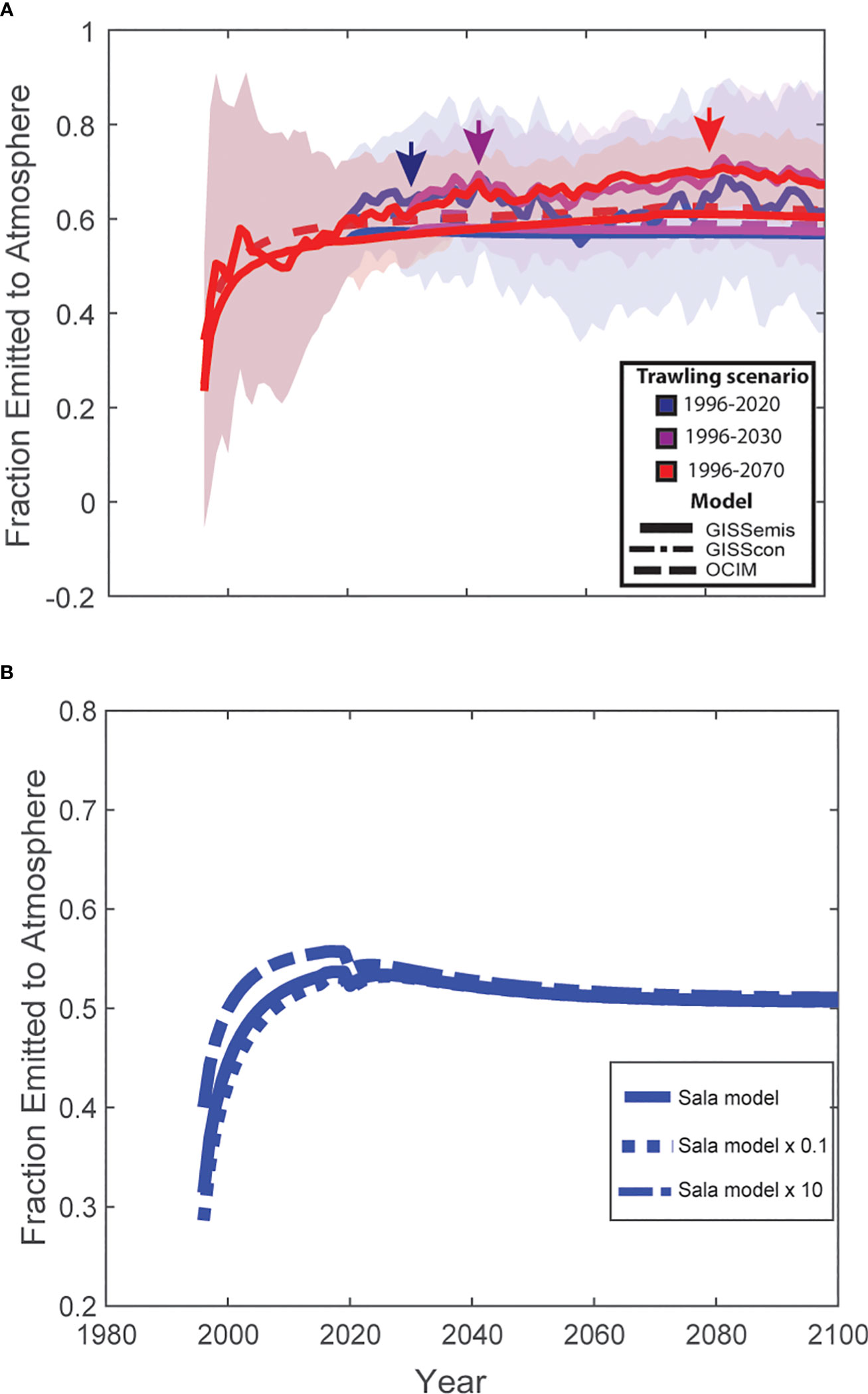
Figure 1 Fraction of trawled CO₂ emitted to the atmosphere. (A) The fraction of trawled CO₂ emitted to the atmosphere from historical trawling (1996-2020) and future projections. Colors represent different trawling scenarios, with blue denoting historical trawling from 1996-2020 and zero trawling thereafter, magenta denoting a future scenario where trawling stops in 2030, and red denoting a future scenario where global trawling ceases in 2070. Continuous lines are ensemble mean solutions from the GISSemis runs, dashed-dotted lines are from the GISScon runs (often not visible in the graph due to overlap with other data points), and dashed lines are from the OCIM simulations. Shading represents the internal variability in the ensemble simulations with the GISSemis model. Arrows indicate when ~99% of the total emissions are released to the atmosphere post-trawling for each of the three trawling scenarios. (B) Effect of the magnitude of CO₂ flux on the fraction of CO₂ emitted to the atmosphere. The solid data line represents the historical (1996-2020) trawling flux estimated using the Sala et al. (2021) carbon model, the dotted lines represent an arbitrarily increase (Sala model x 10) and decrease (Sala model x 0.1) of Sala et al. (2021) flux estimate by one-order of magnitude. Models represent OCIM simulations.

$$fraction (t)=\frac{{\sum }_t\left(FC{O}_{2,trawl}(t)- FC{O}_{2,notrawl}(t)\right)}{{\sum }_{t}BFC{O}_2(t)}$$

where FCO_2,trawl(t) is the globally-integrated atmosphere to ocean CO₂ flux in a simulation with trawling (positive into the ocean), FCO_2,notrawl(t) is the globally-integrated atmosphere to ocean CO₂ flux in the simulation without trawling, and BFCO₂(t) is the globally-integrated benthic emissions of CO₂ due to trawling. Note that FCO_2,notrawl(t) only depends on the model used (GISSemis, GISScon, or OCIM), while FCO_2,trawl(t) and BFCO₂(t) also depends on the trawling scenario considered (historical, trawling ceases in 2030, or trawling ceases in 2070).

2.5 Historical and future changes in pH

To quantify historical changes in pH, we calculated a weighted average of pH in the upper 1000 m of a region. The weighted average is calculated as:

$$p{H}_{ave}=\frac{{\sum }_i(oare{a}_{i}p{H}_i)}{{\sum }_{i}oare{a}_i}$$

where i is an index for location of a model horizontal (lat/lon) grid cell, $oare{a}_i$ is the ocean area of that grid cell, and pH_i is the vertical average of pH in the upper 1000 m of that grid cell. Results for the East China/South China Sea reported in the manuscript are for the average change in pH due to trawling between 2000-2020. We take this as the averaging period to avoid the initial steep decline in pH at the beginning of the simulations, which is likely unrealistic given that trawling activities did exist prior to 1996.

It is important to note that while GISS and OCIM agree on the regions where pH changes are largest, they differ in the magnitude of these changes in some locations. Particularly for the East China/South China Sea, OCIM pH changes are larger than GISSemis changes. These differences likely reflect differences in how trawled carbon data is mapped onto model grids with different bathymetries, particularly as those differences become exaggerated near the coastlines where the majority of trawling is taking place. These differences therefore capture real uncertainty in the pH change in each region, as the models are an imperfect representation of reality. There are also differences in the pH between GISS and OCIM due to differences in their base state chemistry.

2.6 Uncertainty

2.6.1 Trawling intensity

Our estimate of trawling intensity uses a three-dimensional footprint that relies on estimation of both the total area trawled and the penetration depth of bottom trawling gear. We discuss sources of uncertainty relevant to each.

First, our estimate of the area impacted by bottom trawling has three potential sources of uncertainty: (1) uncertainty in the model prediction of active fishing from AIS derived location information, (2) uncertainty in coverage (i.e., what fraction of global trawling is observable via AIS data), and (3) uncertainty in estimated trawl width for each vessel. We have high confidence that bottom trawling fishing activity has been accurately estimated for vessels carrying AIS because Global Fishing Watch’s neural net is notably good at detecting active fishing by trawlers (precision = 0.9, recall = 0.89, and f1-score = 0.89) (Taconet et al., 2019). However, AIS coverage on trawlers < 15 m in total length is low (Taconet et al., 2019); consequently, we underestimate the total footprint of bottom trawling globally because our estimate misses fishing activity from smaller fleets that are not equipped with AIS. Furthermore, the spatial distribution of known gaps in coverage is not uniform. While AIS provides accurate spatial patterns of fishing activity and intensity for some regions (e.g., FAO Area 21, Northwest Atlantic and FAO Area 27, Northeast Atlantic), important gaps in coverage have been identified in the Arctic Sea (FAO Area 18), Western Central Pacific (FAO Area 71), and the Eastern Indian Ocean (FAO Area 57) (Taconet et al., 2019). For example, AIS data are nearly absent from intensely fished regions in Southeast Asia and Indonesia. Additional uncertainty about the area trawled is introduced by our estimate of the width of the trawled gear, for which we use the vessel-size-footprint relationships reported by a study on bottom trawling on the European continental shelf (Eigaard et al., 2016). It is possible that the vessel-size-footprint relationship of the European fleet differs from other global fleets, but these data are not reported elsewhere.

Second, our gear-specific estimates of penetration depth are taken from Hiddink et al. (2017), who use a systematic literature review coupled with a nested linear model to predict the penetration depth for each gear component in each sediment type. Unfortunately, Hiddink et al. (2017) do not elaborate on error and uncertainty in their model for trawl penetration depth.

2.6.2 CO₂ remineralization

Sediment organic carbon stock estimates in the top 1 m horizon were obtained from Atwood et al. (2020), which represents the only study to date to quantify spatially-explicit stocks at a global scale down to 1 m in the sediment; such a depth is required for estimating multiyear impacts of trawling due to annual sedimentation deficits that ultimately require estimates of organic carbon stocks buried in sediment layers that are deeper than the ones immediately impacted by the trawling gear. Atwood et al. (2020) model explained 76% of the variation in organic carbon stocks and had a root-mean-square error of 7306 Mg km⁻². An additional uncertainty in carbon stocks that is acknowledge, but not quantified by Atwood et al. (2020) is variation in carbon stocks with sediment depth. In many cases Atwood et al. (2020) had to extrapolate carbon stocks to 1 m using data from shallower samples.

The largest uncertainty in the CO₂ remineralization model is the estimates of first-order degradation rate constants (k-values). Field studies have shown that k-values can vary substantially both spatially and with depth in the sediment, and unfortunately, studies examining the effects of trawling on organic carbon activity and k-values are extremely limited. We used the k-values published in Sala et al. (2021), which used a literature review and independent validation sites to characterize and generalize region-specific k-values. Across their validation sites, their average model percent error for predicting sediment-water CO₂ fluxes ranged from -45% to +39% when accounting for annual organic carbon flux, with an average absolute error of 23% (Atwood et al., 2023).

It has been suggested by studies that organic carbon reactivity in subsurface sediments could be one to two-orders of magnitude lower than those used in Sala et al. (2021) (Epstein et al., 2022; Hiddink et al., 2023). As a result, we investigated how reductions of one- and two-orders of magnitude in Sala et al. (2021) first-order degradation rates would impact estimated atmospheric emissions. We found that Sala et al. (2021) emission estimates were relatively robust to changes in first-order degradation rates because in the multiyear trawling model, reductions in this parameter substantially reduced carbon depletion through time. Under Sala et al. (2021) original carbon model (global k = 2.6), GISS and OCIM models estimated that trawling emitted as much as ~0.34-0.37 Pg CO₂ yr^-1 to the atmosphere. When first-order degradation rates were reduced by 1-order of magnitude (global average k = 0.28), resulting in only a ~6.8% remineralization efficiency of disturbed organic carbon, the magnitude of atmospheric emissions remained similar to Sala et al (2021) original model (0.19-0.21 Pg CO₂ yr^-1, Atwood et al., 2023). The magnitudes are comparable because in Sala et al, (2021) original model, organic carbon depletion after a decade of trawling results in emissions that are ~27.2% of the year one flux. Conversely, when degradation rates are reduced, more organic carbon stays in the system longer, and changes in trawling-induced fluxes across time stabilize quickly. However, a reduction of the first-order degradation rates by two orders of magnitude (global average k = 0.028; 1.2% remineralization efficiency) does result in a much larger decrease in atmospheric emissions, which are reduced to 0.02-0.03 Pg CO₂ yr^-1 (Atwood et al., 2023), or ~1% of the global emissions from land-use change (Friedlingstein et al., 2020a).

Our models do not account for trawling-induced impacts on organic carbon remineralization due to changes in sediment biota (Epstein et al., 2022). Although the current paradigm in soil science is that microbial communities dominate benthic metabolism in marine sediments, a process that is accounted for in our models, animals undoubtedly play a key role in marine sediment carbon cycling (Snelgrove et al., 2018; LaRowe et al., 2020; Bianchi et al., 2021); yet aquatic and terrestrial animals are universally ignored in Earth Systems Models (Schmitz et al., 2018; Snelgrove et al., 2018; Bianchi et al., 2021). The absence of animals from Earth System Models stems from the lack of generalizable predictions about how animal community changes will likely affect carbon cycling (Schmitz et al., 2018; Schmitz et al., 2023). It can be argued that trawling can stimulate or retard organic carbon remineralization through its differing and often context-dependent effects on infauna communities (Epstein et al., 2022). Yet, the considerable particle mixing and sediment flushing that results from the movement of fishing gear across the seabed could offset some of the potential loss of processes like bioturbation and bioirrigation. Nevertheless, holistic models that include the indirect effects of trawling on organic carbon remineralization through changes in animal communities are needed to make more accurate predictions, especially at smaller spatial scales. However, to better characterize variability and uncertainty in model parameters, further large-scale empirical studies on the biotic and physical processes controlling carbon retention and remineralization in marine sediments, as well as how these processes are affected by trawling, are critical.

2.6.3 Atmospheric emissions

In terms of the response of the global air-sea CO₂ flux to a given trawling emissions pattern, the agreement of the two models suggests that atmospheric emission estimates are fairly robust and inter-model variation is low. Because of the coarse resolution of the models (OCIM: 2° resolution; GISS: 1° x 1.25° resolution), however, regional estimates will have more uncertainty. Thus, the greatest uncertainty in atmospheric emissions estimates comes from the quantification of CO₂ remineralization from trawling impacts on sedimentary carbon (see uncertainties above). Atmospheric emissions and the amount of trawling-induced CO₂ remineralized scale linearly because the air-sea partitioning depends on the circulation timescale and the gas exchange timescale, both of which are unaffected by the relatively small amount of CO₂ emitted by trawling compared to fossil fuel emissions. Therefore, any changes to the amount of trawling-induced CO₂ generated would result in a proportionally similar change in atmospheric CO₂ emissions.

Our models also do not account for the release of N or P from trawled sediments and the potential for those nutrients to stimulate pelagic primary productivity. Unfortunately, there are no global maps of N and P stocks in marine sediments and to our knowledge no empirical studies have explicitly tested this hypothesis. However, modeling studies and theory suggested that if impacts to light attenuation from suspended sediments is short-term, trawling could potentially stimulate primary productivity, and thus uptake of CO₂ (Dounas et al., 2007; Epstein et al., 2022).

2.6.4 Internal climate variability

The GISSemis suite of simulations aims to assess the relative importance of the response to the trawling emissions compared to the system’s internal variability. The ensemble mean is very close to the GISScon and OCIM responses while the internal variability can produce a wide range of individual ensemble member responses that can be ±20% of the ensemble average for the atmospheric CO₂ change and ±40% of the ensemble average for the ocean carbon sink change (see Table S1). However, this uncertainty is model dependent and might be different for other climate models.

3 Results and discussion

Our retrospective and prospective analyses showed that 55-60% of the CO₂ released into the water column by bottom trawling impacts on sediment carbon stocks is emitted to the atmosphere within ~9 years of the trawling event (Figure 1). Furthermore, we found that the fraction of CO₂ accumulating in the atmosphere remained at 55-60% until the end of our simulations at 2100, regardless of the magnitude of CO₂ predicted to be released into the water column by trawling (Figure 1). These results are significant in that they imply that the 55-60% fraction can be easily applied to estimate trawling-induced CO₂ emissions to the atmosphere under a variety of historical and future trawling scenarios.

Using Sala et al. (2021) estimates of sediment efflux, our models suggest that trawling could have emitted a cumulative 8.5-9.2 Pg CO₂ into the atmosphere between 1996 and 2020 (Table S1; Figure 2), contributing 0.97-1.14 ppm to atmospheric CO₂ concentrations (Figure 2). These emissions would equate to ~0.34-0.37 Pg CO₂ yr⁻¹, which is equivalent to ~9-11% of the global emissions from land-use change in 2020 (Friedlingstein et al., 2020b), or nearly double the estimated annual emissions from fuel combustion for the entire global fishing fleet (Parker et al., 2018). Trawling emissions of this magnitude suggest that the protection of seabed organic carbon from benthic trawling gear could prove to be an impactful climate solution. For example, if we continue to trawl at current intensities and spatial distributions, we estimate that bottom trawling could contribute an additional 0.2-0.5 ppm in atmospheric CO₂ concentrations by 2030 and 1.03-1.36 ppm by 2070 (Figure 2).

Figure 2

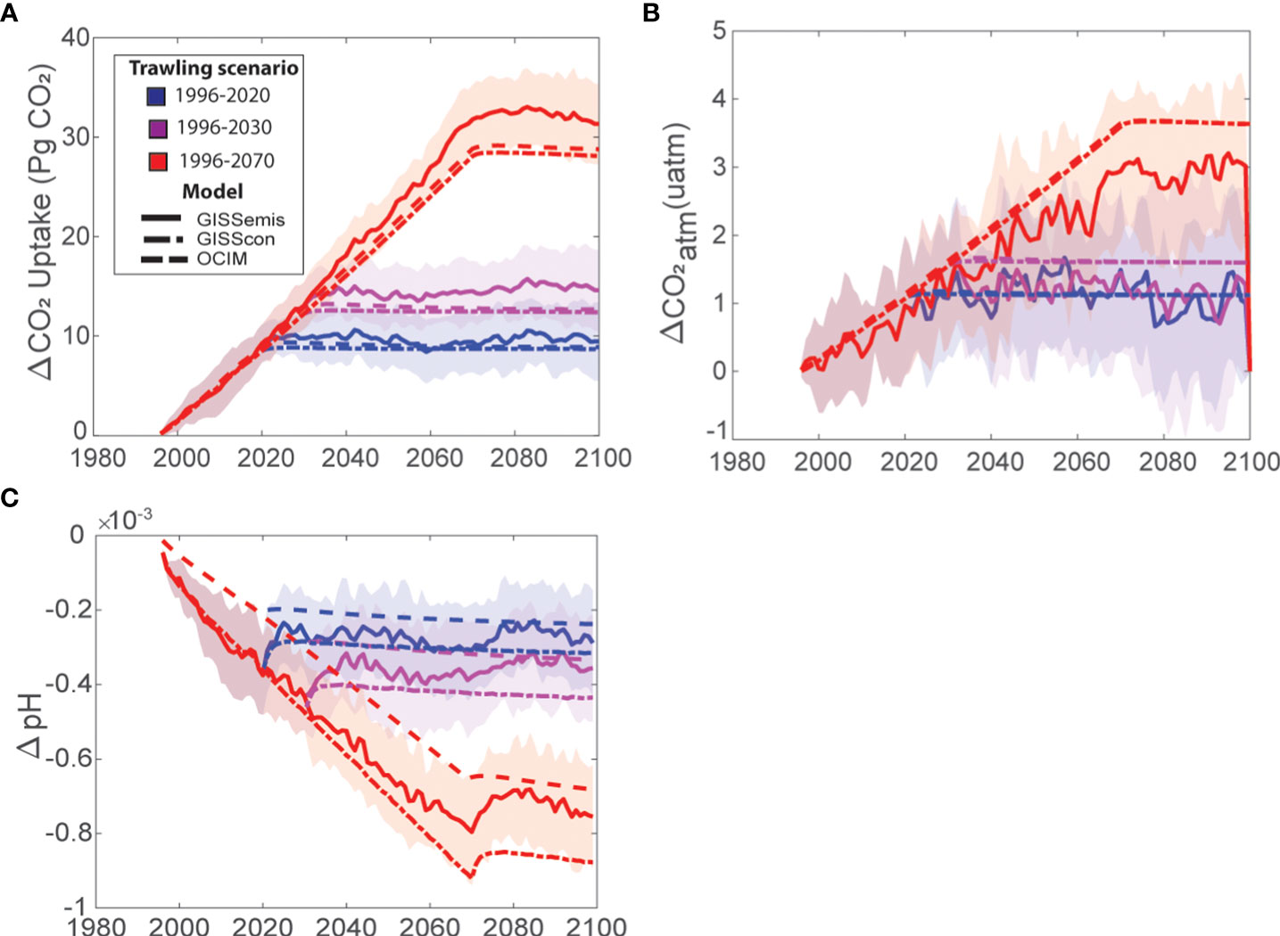
Figure 2 Effects of benthic trawling on CO₂ emissions and bottom water pH. Time series of the (A) change in cumulative carbon uptake by the ocean due to trawling, or equivalently a flux of CO₂ to the atmosphere, (B) change in atmospheric CO₂ concentrations due to trawling in the different model simulations (OCIM, GISScon, GISSemis), and (C) global ocean pH change due to trawling. Colors represent different trawling scenarios, with blue denoting historical trawling from 1996-2020 and zero trawling thereafter, magenta denoting a future scenario where trawling stops in 2030, and red denoting a future scenario where global trawling ceases in 2070. Continuous lines are ensemble mean solutions from the GISSemis runs, dashed-dotted lines are from the GISScon runs, and dashed lines are from the OCIM simulations. Shading represents the internal variability in the ensemble simulations with the GISSemis model.

Whether or not reductions in trawling could be adapted as a climate solution not only depends on the magnitude of the emission reductions, but also the time frame over which those reductions can be achieved. We found that the release of trawling-induced CO₂ from the ocean to the atmosphere occurred rapidly, with ~99% of the total emissions occurring within 7-9 years post-bottom trawling (OCIM: 7 yrs; GISScon: 9 yrs; GISSemis: 9 yrs ± 5 yrs (standard deviation of ensemble members). When emissions were arbitrarily increased by one order of magnitude, it took slightly less time (OCIM:~5 yrs) for total emissions to be released into the atmosphere. The rapid release of CO₂ from the ocean to the atmosphere suggests that historical trawling has only short-term legacy effects on atmospheric emissions. Thus, policies that eliminate or significantly limit trawling impacts on sedimentary carbon stocks would quickly reduce this industry’s contribution to rising atmospheric CO₂ concentrations with maximum benefits occurring 7-9 years after implementation.

In general, atmospheric CO₂ emission hotspots coincided with areas where trawling had the most significant impact on benthic carbon, mainly the East China Sea, the Baltic and the North Sea, and the Greenland Sea (Figure 3). However, horizontal advection can transport trawling-induced CO₂ and resuspended organic carbon to other locations, leading to cross-boundary effects of bottom trawling on local carbon cycles. This phenomenon likely explains why some areas such as the South China Sea, Norwegian Sea, and off the east coast of Japan in the Pacific Ocean had higher atmospheric emissions than expected based on the local rate of trawling emissions (Figure 3). As a result of these cross-boundary effects, we cannot assume that all the atmospheric emissions within a country’s jurisdictional waters come from trawling activities within that zone.

Figure 3

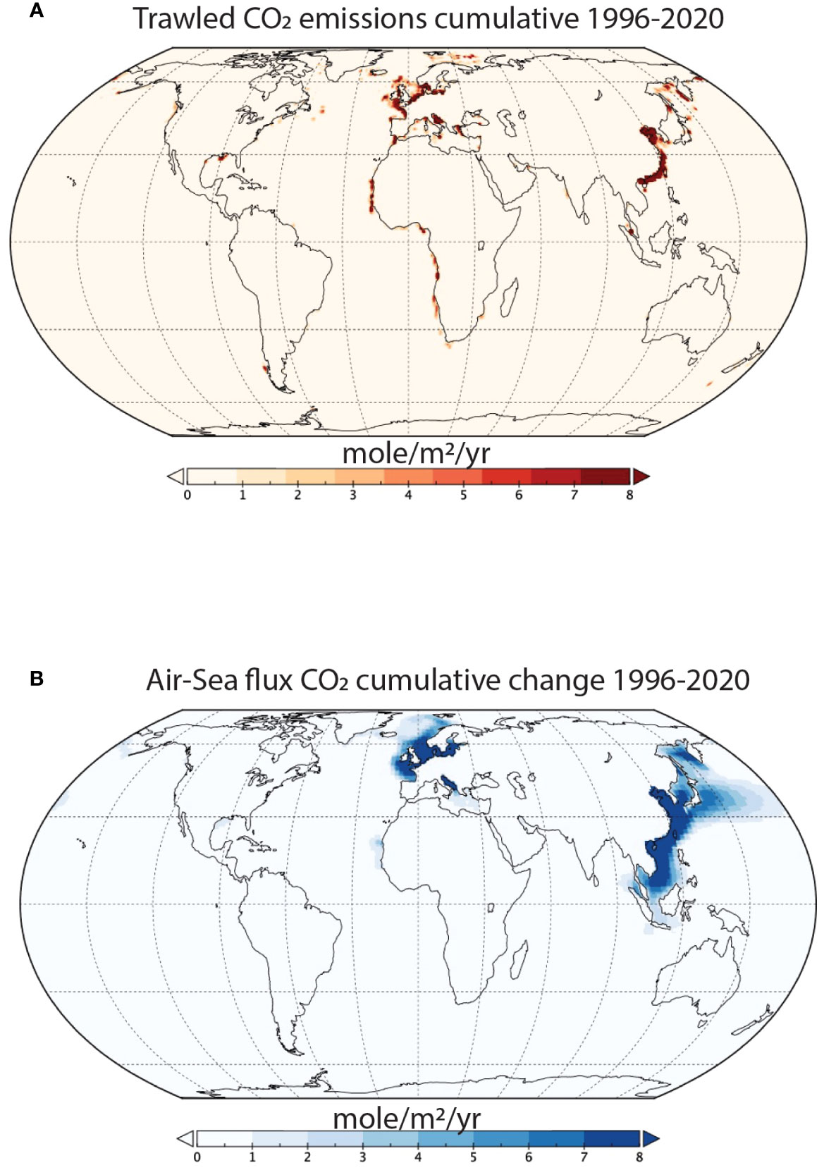
Figure 3 Spatial differences in the historical effects of benthic trawling on CO₂ emissions. (A) Cumulative emissions of trawled CO₂ between 1996-2020. (B) Cumulative changes in the air-sea CO₂ flux due to trawling between 1996-2020. It is important to note that significant knowledge gaps exist regarding trawling activity in the Arctic Sea (FAO Area 18), Western Central Pacific (FAO Area 71), and the Eastern Indian Ocean (FAO Area 57) (Taconet et al., 2019). Consequently, emissions attributed to trawling in these regions are likely underestimated.

Our ability to quantify the extent of the global bottom trawling fleet through time and space in this study was somewhat limited. Our estimates do not capture trawling activities before 1996, because the intensity and spatial distribution of bottom trawling before that time are unknown. Yet, large-scale bottom trawling began as early as 1950 and peaked in the 1980s and 1990s (Watson et al., 2006; Watson and Tidd, 2018). Furthermore, our model relies on the AIS vessel tracking database processed by Global Fishing Watch (https://globalfishingwatch.org/) to derive trawling events at the global level. Unfortunately, AIS coverage is poor in some fishing-intensive areas. Thus, we undoubtedly underestimate trawling activity in areas of Southeast Asia, the Bay of Bengal, the Arabian Sea, parts of Europe, and the Gulf of Mexico (Taconet et al., 2019).

There are additional uncertainties in the parameters used to estimate the amount of organic carbon remineralized after trawling due to a lack of rigorous field studies. Though our model is parameterized using the best available empirical data (Sala et al., 2021; Atwood et al., 2023), an alternative line of reasoning argues that first-order degradation rates could be one- to two orders of magnitude lower (Hiddink et al., 2023). Because we find that atmospheric emissions scale linearly with the amount of organic carbon remineralized to aqueous CO₂ by trawling, we can straightforwardly examine the sensitivity of our results to this alternative assumption. Leveraging Atwood et al. (2023) finding that reducing first-order degradation rates by one order of magnitude has a negligible effect on the estimated magnitude of organic carbon remineralized after 10 consecutive years of trawling, we find that retaining this reduction to first-order degradation rates results in an estimated 0.19-0.21 Pg CO₂ yr^-1 emitted to the atmosphere due to bottom trawling between 1996-2020. A two-orders of magnitude reduction to first-order degradation would result in 0.02-0.03 Pg CO₂ yr^-1 emitted over the same time period – comparable to the mitigation potential for managing fires in temperate forests (Griscom et al., 2017).

Currently, climate actions aimed at reducing CO₂ emissions from anthropogenic practices (e.g., carbon markets, renewable energy standards, reforestation efforts, etc.) focus exclusively on atmospheric emissions. However, these frameworks overlook the total impact of ocean-use change activities on the carbon cycle, because they ignore the pool of DIC that remains sequestered by the ocean. In the case of trawling, we found that 40-45% of the cumulative trawling-induced CO₂ emissions remained dissolved in seawater, augmenting the acidification already occurring from the burning of fossil fuels. Using Sala et al. (2021) carbon model, we found that trawling increased the global DIC inventory by ~1.82-1.90 Pg C from 1996-2020 (Table S1). This additional dissolved inorganic carbon from trawling results in increased ocean acidification with a global reduction in pH of 3-5 ×10^-4 by 2020 (Figure 2). At the global scale, a pH reduction of that magnitude by 2020 is not significant compared to the effect of anthropogenic emissions due to fossil fuels. However, our models suggest that some semi-enclosed seas could be highly sensitive to an injection of CO₂ from anthropogenic activities. In particular, our models showed that extensive trawling could lead to increased localized acidification in the East and South China Sea (Figure 4). The decrease in pH in this region due to trawling between 2000 and 2020 (GISSemis: -0.034+/-0.001; OCIM: -0.050) is comparable to that from rising atmospheric CO₂ due to the burning of fossil fuels over the same time period (GISSemis: -0.034+/-0.004; OCIM: -0.020). An important caveat to our pH findings is that our models are limited in resolving coastal processes both due to their coarse resolution and lack of biogeochemical complexity. Nevertheless, considering that ocean chemistry can influence organismal development, physiology, and behavior (Baag and Mandal, 2022), and ultimately can affect a species’ productivity and survival, future studies and policy should consider the potential impacts trawling can have on localized ocean acidification.

Figure 4

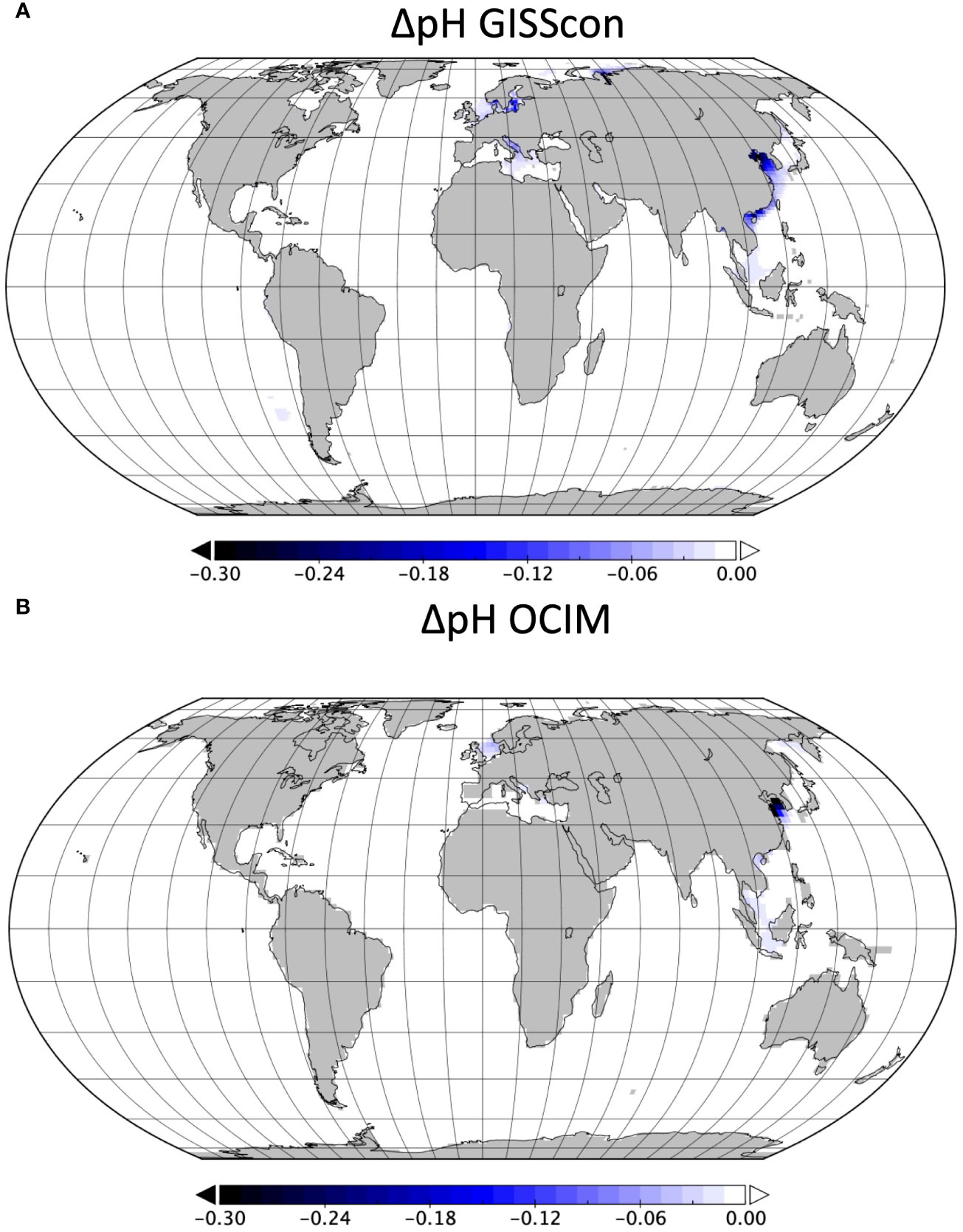
Figure 4 Spatial differences in the historical effects of benthic trawling on pH. Change in upper 1000-m average pH due to trawling in 2020 for (A) GISScon Model results and (B) OCIM Model results.

4 Conclusion

Ocean-based solutions offer promise in closing the emissions gap to limit global temperature increases to 1.5°C, while also supporting co-benefits like biodiversity preservation and food security (Hoegh-Guldberg et al., 2019; Sala et al., 2021). However, current climate policies and markets require estimates of avoided atmospheric emissions, posing challenges for identifying and implementing these solutions. Our study, which highlights that 55-60% of CO₂ produced from bottom trawling is released into the atmosphere within nine years, becomes a crucial tool for evaluating the reduction of bottom trawling effort as an effective ocean-based climate solution. To refine atmospheric emission estimates, it is essential for field studies to tackle uncertainties in our understanding of how bottom trawling influences the biological and physical processes that govern carbon remineralization and preservation. Furthermore, the incorporation of high-resolution regional models that resolve small-scale processes, such as local currents, will be pivotal in delivering more precise emission estimates at scales pertinent to local policy considerations. Lastly, our findings emphasize the need for policy to avoid exclusive focus on avoided atmospheric emissions, as our results show that trawling-induced increases in DIC in seawater could have severe implications for local or regional ocean acidification.

Data availability statement

The datasets presented in this study can be found in online repositories. The names of the repository/repositories and accession number(s) are as follows. Data on marine sedimentary carbon stocks is available at https://figshare.com/articles/dataset/marine_soil_carbon/9941816. Data on swept volume ratios and trawling activity are available by contacting Global Fishing research@globalfishingwatch.org. The code for GISS models is available at the TrawlingExpts2023 at http://simplex.giss.nasa.gov; for access to the simplex.giss.nasa.gov repository, email anastasia.romanou@nasa.gov. OCIM code is available upon email request to TD at tdevries@geog.ucsb.edu. All data used for this study and the figures can be found in the NASA Center for Climate Simulation portal: https://portal.nccs.nasa.gov/datashare/modelE_ocean/Atwood_etal2023_paper_data.

Author contributions

All authors contributed to the conceptualization and design of the study. AR, PL, TD, and JM ran data analyses. TA wrote the original draft of the manuscript and all authors contributed to reviewing and editing. All authors contributed to the article and approved the submitted version.

Funding

The author(s) declare financial support was received for the research, authorship, and/or publication of this article. TA, JM, DB, RC, and ES acknowledge funding from National Geographic Pristine Seas. TA was funded by an Early Career Research Fellowship from the Gulf Research Program of the National Academies of Sciences, Engineering, and Medicine (The content is solely the responsibility of the authors and does not necessarily represent the official views of the Gulf Research Program of the National Academies of Sciences, Engineering, and Medicine). TD was funded by the National Science Foundation under grant OCE-1948955. AR, PL, and GS were supported by the Modeling, Analysis and Prediction Program from NASA and by the High-End Computing Program through the NASA Center for Climate Simulation at Goddard Space Flight Center.

Acknowledgments

We thank Y. Rousseau for insights on temporal patterns in trawling.

Conflict of interest

The authors declare that the research was conducted in the absence of any commercial or financial relationships that could be construed as a potential conflict of interest.

Publisher’s note

All claims expressed in this article are solely those of the authors and do not necessarily represent those of their affiliated organizations, or those of the publisher, the editors and the reviewers. Any product that may be evaluated in this article, or claim that may be made by its manufacturer, is not guaranteed or endorsed by the publisher.

Supplementary material

The Supplementary Material for this article can be found online at: https://www.frontiersin.org/articles/10.3389/fmars.2023.1125137/full#supplementary-material

References

Amoroso R. O., Pitcher C. R., Rijnsdorp A. D., McConnaughey R. A., Parma A. M., Suuronen P., et al. (2018). ). Bottom trawl fishing footprints on the world’s continental shelves. Proc. Natl. Acad. Sci. 115, E10275–E10282. doi: 10.1073/pnas.1802379115

CrossRef Full Text | Google Scholar

Atwood T., Sala E., Mayorga J., Bradley D., Cabral R. B., Auber A., et al. (2023). Response to comment on “Quantifying the carbon benefits of ending bottom trawling. Nature 617, E3–E5. doi: 10.1038/s41586-023-06015-6

PubMed Abstract | CrossRef Full Text | Google Scholar

Atwood T. B., Witt A., Mayorga J., Hammill E., Sala E. (2020). Global patterns in marine sediment carbon stocks. Front. Mar. Sci. 7. doi: 10.3389/fmars.2020.00165

CrossRef Full Text | Google Scholar

Baag S., Mandal S. (2022). Combined effects of ocean warming and acidification on marine fish and shellfish: A molecule to ecosystem perspective. Sci. Total Environ. 802. doi: 10.1016/j.scitotenv.2021.149807

PubMed Abstract | CrossRef Full Text | Google Scholar

Bianchi T. S., Aller R. C., Atwood T. B., Brown C. J., Buatois L. A., Levin L. A., et al. (2021). What global biogeochemical consequences will marine animal-sediment interactions have during climate change. Elem. Sci. Anth. 9, 1–25. doi: 10.1525/elementa.2020.00180

CrossRef Full Text | Google Scholar

Burdige D. J. (2007). Preservation of organic matter in marine sediments: Controls, mechanisms, and an imbalance in sediment organic carbon budgets? Chem. Rev. 107, 467–485. doi: 10.1021/cr050347q

PubMed Abstract | CrossRef Full Text | Google Scholar

DeVries T. (2014). The oceanic anthropogenic CO2 sink: Storage, air-sea fluxes, and transports over the industrial era. Global Biogeochem. Cycles 28, 631–647. doi: 10.1002/2013GB004739

CrossRef Full Text | Google Scholar

Dounas C., Davies I., Triantafyllou G., Koulouri P., Petihakis G., Arvanitidis C., et al. (2007). Large-scale impacts of bottom trawling on shelf primary productivity. Cont. Shelf Res. 27, 2198–2210. doi: 10.1016/j.csr.2007.05.006

CrossRef Full Text | Google Scholar

Eigaard O. R., Bastardie F., Breen M., Dinesen G. E., Hintzen N. T., Laffargue P., et al. (2016). Estimating seabed pressure from demersal trawls, seines, and dredges based on gear design and dimensions. ICES J. Mar. Sci. 73, i27–i43. doi: 10.1093/icesjms/fsv099

CrossRef Full Text | Google Scholar

Epstein G., Middelburg J. J., Hawkins J. P., Norris C. R., Roberts C. M. (2022). The impact of mobile demersal fishing on carbon storage in seabed sediments. Glob. Change Biol. 28, 2875–2894. doi: 10.1111/gcb.16105

CrossRef Full Text | Google Scholar

Friedlingstein P., O’Sullivan M., Jones M., Andrew R., Hauck J., Olsen A., et al. (2020a). Global carbon budget 2021. Preprint 10.5194/es, 1–3. doi: 10.5194/essd-2020-286

CrossRef Full Text | Google Scholar

Friedlingstein P., O’Sullivan M., Jones M. W., Andrew R. M., Hauck J., Olsen A., et al. (2020b). Global carbon budget 2020. Earth Syst. Sci. Data 12, 3269–3340. doi: 10.5194/essd-12-3269-2020

CrossRef Full Text | Google Scholar

Garcia H. E., Weathers K. W., Paver C. R., Smolyar I. V., Boyer T. P., Locarnini R. A., et al. (2019). “Dissolved inorganic nutrients (phosphate, nitrate and nitrate + nitrite, silicate,” in World atlas 2018. Ed. Mishonov A. V. (Silver Springs, MD: USA Department of Commerce), 35. NOAA Atlas NESDIS 84.

Google Scholar

Gregg W. W., Casey N. W. (2007). Modeling coccolithophores in the global oceans. Deep. Res. Part II Top. Stud. Oceanogr. 54, 447–477. doi: 10.1016/j.dsr2.2006.12.007

CrossRef Full Text | Google Scholar

Griscom B. W., Adams J., Ellis P. W., Houghton R. A., Lomax G., Miteva D. A., et al. (2017). Natural climate solutions. Proc. Natl. Acad. Sci. 114, 11645–11650. doi: 10.1073/pnas.1710465114

CrossRef Full Text | Google Scholar

Hiddink J. G., Jennings S., Sciberras M., Szostek C. L., Hughes K. M., Ellis N., et al. (2017). Global analysis of depletion and recovery of seabed biota after bottom trawling disturbance. Proc. Natl. Acad. Sci. U.S.A. 114, 8301–8306. doi: 10.1073/pnas.1618858114

PubMed Abstract | CrossRef Full Text | Google Scholar

Hiddink J. G., van de Velde S., McConnaughey R. A., De Borger E., O’Neill F. G., Tiano J., et al. (2023). Quantifying the carbon benefits of ending bottom trawling. Nature 617, E1–E2. doi: 10.1038/s41586-023-06014-7

PubMed Abstract | CrossRef Full Text | Google Scholar

Hoegh-Guldberg O., Northrop E., Lubchenco J. (2019). The ocean is key to achieving climate and societal goal. Science 365, 1372–1374. doi: 10.1126/science.aaz4390

PubMed Abstract | CrossRef Full Text | Google Scholar

Holzer M., DeVries T., de Lavergne C. (2021). Diffusion controls the ventilation of a Pacific Shadow Zone above abyssal overturning. Nat. Commun. 12, 1–13. doi: 10.1038/s41467-021-24648-x

PubMed Abstract | CrossRef Full Text | Google Scholar

IPCC (2022). Climate change 2022: impacts, adaptation, and vulnerability. contribution of working group ii to the sixth assessment report of the intergovernmental panel on climate change. Pörtner H.-O., Roberts D. C., Tignor M., Poloczanska E. S., Mintenbeck K., Alegría A., Craig M., Langsdorf S., Löschke S., Möller V., Okem A., Rama B. (eds.). (Cambridge, UK and New York, NY, USA: Cambridge University Press), 3056 pp. doi: 10.1017/9781009325844

CrossRef Full Text | Google Scholar

Ito G., Romanou A., Kiang N. Y., Faluvegi G., Aleinov I., Ruedy R., et al. (2020). Global carbon cycle and climate feedbacks in the NASA GISS ModelE2.1. J. Adv. Model. Earth Syst. 12, 1–44. doi: 10.1029/2019MS002030

CrossRef Full Text | Google Scholar

LaRowe D. E., Arndt S., Bradley J. A., Estes E. R., Hoarfrost A., Lang S. Q., et al. (2020). The fate of organic carbon in marine sediments - New insights from recent data and analysis. Earth-Science Rev. 204, 103146. doi: 10.1016/j.earscirev.2020.103146

CrossRef Full Text | Google Scholar

Lerner P., Romanou A., Kelley M., Romanski J., Ruedy R., Russell G. (2021). Drivers of air-sea CO2 flux seasonality and its long-term changes in the NASA-GISS model CMIP6 submission. J. Adv. Model. Earth Syst. 13, 1–33. doi: 10.1029/2019MS002028

CrossRef Full Text | Google Scholar

Levin L. A., Wei C. L., Dunn D. C., Amon D. J., Ashford O. S., Cheung W. W. L., et al. (2020). Climate change considerations are fundamental to management of deep-sea resource extraction. Glob. Change Biol. 26, 4664–4678. doi: 10.1111/gcb.15223

CrossRef Full Text | Google Scholar

Locarnini R. A., Mishonov A. V., Baranova O. K., Boyer T. P., Zweng M. M., Garcia H. E., et al. (2019). World ocean atlas 2018 , volume 1: temperatureEd.Mishonov A. (Silver Springs, MD: USA Department of Commerce).

Google Scholar

Luisetti T., Ferrini S., Grilli G., Jickells T. D., Kennedy H., Kröger S., et al. (2020). Climate action requires new accounting guidance and governance frameworks to manage carbon in shelf seas. Nat. Commun. 11, 1–10. doi: 10.1038/s41467-020-18242-w

PubMed Abstract | CrossRef Full Text | Google Scholar

Meinshausen M., Nicholls Z., Lewis J., Gidden M., Vogel E., Freund M., et al. (2020). The SSP greenhouse gas concentrations and their extensions to 2500. Geosci. Model. Dev. Discuss. 13, 3571–3605. doi: 10.5194/gmd-13-3571-2020

CrossRef Full Text | Google Scholar

Miller R. L., Schmidt G. A., Nazarenko L. S., Bauer S. E., Kelley M., Ruedy R., et al. (2021). CMIP6 historical simulations, (1850–2014) with GISS-E2.1. J. Adv. Model. Earth Syst. 13, 1–35. doi: 10.1029/2019MS002034

CrossRef Full Text | Google Scholar

Najjar R., Orr J. (1999). “Design of ocmip-2 simulations of chlorofluorocarbons, the solubility pump and common biogeochemistry [OCMIP-2 Protocols],” in OCMIP web applications. (Silver Springs, MD: USA Department of Commerce). Available at: http://ocmip5.ipsl.fr/documentation/OCMIP/phase2/.

Google Scholar

Olsen A., Key R. M., Van Heuven S., Lauvset S. K., Velo A., Lin X., et al. (2016). The global ocean data analysis project version 2 (GLODAPv2) - An internally consistent data product for the world ocean. Earth Syst. Sci. Data 8, 297–323. doi: 10.5194/essd-8-297-2016

CrossRef Full Text | Google Scholar

O’Neill B. C., Tebaldi C., Van Vuuren D. P., Eyring V., Friedlingstein P., Hurtt G., et al. (2016). The scenario model intercomparison project (ScenarioMIP) for CMIP6. Geosci. Model. Dev. 9, 3461–3482. doi: 10.5194/gmd-9-3461-2016

CrossRef Full Text | Google Scholar

Orr J. C., Najjar R. G., Aumont O., Bopp L., Bullister J. L., Danabasoglu G., et al. (2017). Biogeochemical protocols and diagnostics for the CMIP6 ocean model intercomparison project (OMIP). J. Geophys. Res. Atmos. 112, 2169–2199. doi: 10.1029/2007JD008643

CrossRef Full Text | Google Scholar

Paradis S., Goñi M., Masqué P., Durán R., Arjona-Camas M., Palanques A., et al. (2021). Persistence of biogeochemical alterations of deep-sea sediments by bottom trawling. Geophys. Res. Lett. 48, 1–12. doi: 10.1029/2020gl091279

CrossRef Full Text | Google Scholar

Parker R. W. R., Blanchard J. L., Gardner C., Green B. S., Hartmann K., Tyedmers P. H., et al. (2018). Fuel use and greenhouse gas emissions of world fisheries. Nat. Clim. Change 8, 333–337. doi: 10.1038/s41558-018-0117-x

CrossRef Full Text | Google Scholar

Pauly D., Zeller D., Palomares M. L. D. (2020). Sea around us concepts, design and data. (Silver Springs, MD: USA Department of Commerce).

Google Scholar

Romanou A., Gregg W. W., Romanski J., Kelley M., Bleck R., Healy R., et al. (2013). Natural air-sea flux of CO2 in simulations of the NASA-GISS climate model: Sensitivity to the physical ocean model formulation. Ocean Model. 66, 26–44. doi: 10.1016/j.ocemod.2013.01.008

CrossRef Full Text | Google Scholar

Rousseau Y., Watson R. A., Blanchard J. L., Fulton E. A. (2019). Evolution of global marine fishing fleets and the response of fished resources. Proc. Natl. Acad. Sci. U.S.A. 116, 12238–12243. doi: 10.1073/pnas.1820344116

PubMed Abstract | CrossRef Full Text | Google Scholar

Sala E., Mayorga J., Bradley D., Cabral R. B., Atwood T. B., Auber A., et al. (2021). Protecting the global ocean for biodiversity, food and climate. Nature 592, E25. doi: 10.1038/s41586-021-03496-1

PubMed Abstract | CrossRef Full Text | Google Scholar

Schmitz O. J., Sylvén M., Atwood T. B., Bakker E. S., Berzaghi F., Brodie J. F., et al. (2023). Trophic rewilding can expand natural climate solutions. Nat. Clim. Chang. 13, 324–333. doi: 10.1038/s41558-023-01631-6

CrossRef Full Text | Google Scholar

Schmitz O. J., Wilmers C. C., Leroux S. J., Doughty C. E., Atwood T. B., Galetti M., et al. (2018). Animals and the zoogeochemistry of the carbon cycle. Sci. (80-. ). 362, eaar3213. doi: 10.1126/science.aar3213

CrossRef Full Text | Google Scholar

Siegel D. A., Devries T., Doney S. C., Bell T. (2021). Assessing the sequestration time scales of some ocean-based carbon dioxide reduction strategies. Environ. Res. Lett. 16, 104003. doi: 10.1088/1748-9326/ac0be0

CrossRef Full Text | Google Scholar

Snelgrove P. V. R., Soetaert K., Solan M., Thrush S., Wei C. L., Danovaro R., et al. (2018). Global carbon cycling on a heterogeneous seafloor. Trends Ecol. Evol. 33, 96–105. doi: 10.1016/j.tree.2017.11.004

PubMed Abstract | CrossRef Full Text | Google Scholar

Taconet M., Kroodsma D., Fernandes J. A. (2019). Global atlas of AIS-based fishing activity-Challenges and opportunities (FAO: Rome).

Google Scholar

van Heuven S., Pierrot D., Rae J. W. B., Lewis E., Walace D. W. R. (2011). CO2SYS v 1.1 : MATLAB program developed for CO2 system calculations. ORNL/CDIAC-105b. (Silver Springs, MD: USA Department of Commerce). doi: 10.3334/CDIAC/otg.CO2SYS_MATLAB_v1.1

CrossRef Full Text | Google Scholar

Watson R. A. (2017). A database of global marine commercial, small-scale, illegal and unreported fisheries catch 1950-2014. Sci. Data 4, 1–9. doi: 10.1038/sdata.2017.39

CrossRef Full Text | Google Scholar

Watson R., Revenga C., Kura Y. (2006). Fishing gear associated with global marine catches. II. Trends in trawling and dredging. Fish. Res. 79, 103–111. doi: 10.1016/j.fishres.2006.01.013

CrossRef Full Text | Google Scholar

Watson R. A., Tidd A. (2018). Mapping nearly a century and a half of global marine fishing: 1869–2015. Mar. Policy 93, 171–177. doi: 10.1016/j.marpol.2018.04.023

CrossRef Full Text | Google Scholar

Wilkinson G. M., Besterman A., Buelo C., Gephart J., Pace M. L. (2018). A synthesis of modern organic carbon accumulation rates in coastal and aquatic inland ecosystems. Sci. Rep. 8, 1–9. doi: 10.1038/s41598-018-34126-y

PubMed Abstract | CrossRef Full Text | Google Scholar

Zweng M. M., Reagan J. R., Seidov D., Boyer T. P., Locarnini R. A., Garcia A. V., et al. (2018). World ocean atlas 2018 volume 2 : salinityEd. Mishonov A. (Silver Springs, MD: USA Department of Commerce).

Google Scholar