A regional map of mangrove extent for Myanmar, Thailand, and Cambodia shows losses of 44% by 1996

1 Introduction

Mangroves contribute up to 10–15% of global carbon storage for coastal oceans and up to 10–11% of biogeophysical coastal carbon cycling (Bouillon et al., 2008; Alongi, 2014; Simard et al., 2019). This makes them one of the most carbon-rich and carbon-sequestering forests with the potential to mitigate climate change and biodiversity loss (Donato et al., 2011; Howard et al., 2017; Adame et al., 2021). They are also essential to biogeochemical processes, erosion prevention, sedimentation, protection against extreme weather events, and support for coastal cultures and economies (Singh et al., 2005; Brander et al., 2012). Altogether, the ecosystem services provided by mangroves have been estimated at $1.6 billion per year (Polidoro et al., 2010). Although land managers and coastal community members have understood their value, some studies have estimated a total mangrove carbon stock decline of 158.4 Mt over the course of 1996 to 2016 (Richards et al., 2020).

Fortunately, the continuity of satellite data has enabled important insight on mangrove change dynamics. The Landsat program provides the most continuous terrestrial remote sensing records that span the last 50 years (Loveland and Dwyer, 2012; Wang et al., 2019; Yan and Roy, 2021). The Landsat repository has proven fundamental to mapping the distribution and change of mangrove forests around the world (Spalding et al., 2010; Giri et al., 2011; Hamilton and Casey, 2016; Goldberg et al., 2020; Bunting et al., 2022; Murray et al., 2022). Globally, the Landsat archive has recorded an estimated global loss of 20–35% since 1980 (Valiela et al., 2001; Polidoro et al., 2010) with estimated rates of loss between −0.16% and −3.4% (Hamilton and Casey, 2016; Bunting et al., 2022), yet many studies also document high rates of variability. One study found that various changes were often at odds with one another: in some cases even the direction of change was inconsistent among datasets Friess and Webb, 2014. Estimates of mangrove loss depend on the availability, observation period, and spatial coverage of mangrove data products (Gibbs et al., 2007; Friess and Webb, 2014) to reduce this variability. As a result, we speculate that estimates of historical rates of loss before the turn of the 21^st century are not well-constrained (Everitt and Judd, 1989; Wang et al., 2019; Lewis and MacDonald, 1972; Lorenzo et al., 1979) due to four primary reasons: the challenges of working with earlier EO data (Faundeen et al., 2004; Pasquarella et al., 2016), region-specific conflicts that reduced the historical capacity for research (Han et al., 2020; Lekfuangfu and Nakavachara, 2021), the subsequent lack of remotely sensed mangrove extent data products (Wulder et al., 2016; Hu et al., 2018), and a resulting dependence on unreliable reporting of spatial extents (Friess and Webb, 2014; Wang et al., 2019). As we embark on the UN Decade on Ecosystem Restoration, we hope to enhance ongoing conversations on the historical changes of mangrove extent by filling this research gap in the literature.

The challenge with integrating earlier sensors is related to a historical lack of accessibility and limitations with the Landsat 1-5 Multispectral Scanner System (LMSS) (U.S. Geological Survey, Department 2018) and other remotely sensed observations. Individual use of Landsat imagery was severely limited until Landsat transitioned to a free and open data policy in 2008 (Pasquarella et al., 2016; Zhu et al., 2019). The high demand for Landsat data has led to improvements in calibration and corrections across various sensors, but only 49% of this satellite repository has been corrected to its highest level of precision and terrain processing (L1TP) which is characterized by its well-adjusted radiometry and inter-sensor capacity for calibration (U.S. Geological Survey, Department 2018; Yan and Roy, 2021). The remaining images in the archive have been processed to the lower L1G level of correction given the lack of elevation data and ground control references that the Level 1 Product Generation System requires (Devaraj and Shah, 2014; U.S. Geological Survey Department, 2018). Radiometric calibration that meets research standards is critical to developing the modeling methodologies that can be applied consistently over different scenes and image dates when conducting mangrove mapping projects.

As a result, most global and regional mangrove mapping efforts only date back to 2000, with a few extending into the 1990s (Bunting et al., 2022; Murillo-Sandoval et al., 2022; Hamilton and Stankwitz, 2012), which can influence conservation decision making and outcomes (Friess and Webb, 2014; Hamilton et al., 2018; Dahdouh-Guebas and Cannicci, 2021). One such study (Dahdouh-Guebas and Cannicci, 2021) made the distinction that a variety of rehabilitation and restoration targets on mangrove health assessments rely on the earliest available earth observation or past vegetation dataset to establish which areas can be sustainably rejuvenated and which are a restoration priority (Wang et al., 2019; Dahdouh-Guebas and Cannicci, 2021). Although mangrove remote sensing can be traced back to the 1970s (Kuenzer et al., 2011), they are few, the majority were completed without accuracy assessments, or were restricted to sub-regional spatial coverages (Lorenzo et al., 1979; Lewis and MacDonald, 1972; Everitt and Judd, 1989; Islam et al., 2019; Wang et al., 2019). Albeit one of the more extensive mapping efforts executed by Giri et al. (2008) were able to map country-wide mangrove changes for the tsunami affected regions of Asia (including Thailand and Myanmar) at three epochs over the course of 1975 to 2005. Furthermore, by 2018, over 435 publications had been completed enumerating the extent of mangrove ecosystems, but literature gaps remained from 1972 to 1995 (Kuenzer et al., 2011; Wang et al., 2019) with little to none of the publications utilizing wall to wall LMSS coverage for regions in Southeast Asia (Lorenzo et al., 1979; Reddy et al., 2007; Rahman, 2012; Li et al., 2013; Son et al., 2014; Islam et al., 2019).

As a consequence, our understanding of mangrove rates of change before the 1990s are variable. According to multiple comprehensive reviews on the remote sensing of mangrove extent and change (Hu et al., 2018; Friess et al., 2019; Wang et al., 2019), there is high uncertainty in both regional and global estimates. Historical and predicted estimates of change over time can therefore result in conflicting deforestation and afforestation trends depending on the datasets used in the models (Friess and Webb, 2014). Detailed reporting on mangrove area approximations are error-prone due to their dependence on coarse resolution surveys and inconsistent methods (Hu et al., 2018; Friess et al., 2019). As such, there is a need to utilize the full capacity of EO to more accurately observe mangrove forests earlier in the satellite record, particularly those with historically high and uncertain rates of deforestation.

Southeast Asia contains the greatest proportion of mangrove area (34%) in the world (Thomas et al., 2017; Bunting et al., 2022), but aquaculture, mining, agriculture, and urban expansion threaten these mangroves (Worthington and Spalding, 2018; Richards and Friess, 2016; DeFries et al., 2010; Webb et al., 2014; Friess et al., 2016). To the best of our knowledge, there are little to no studies using LMSS L1T Tier 2 Collection 1 Level 1 Raw DN observations to both map and report on the extent of mangroves for Thailand, Myanmar, and Cambodia in the 1970s. This means that national and international reporting on the net losses of mangrove extent rely on estimates from the Food and Agriculture Organization (2007; Friess et al., 2019) which contribute to contradictory deforestation rates in the mainland of Southeast Asia. For Thailand and Myanmar, studies report rates of change with a range of 7.08 ± 42.99 km² yr⁻¹ and −60.61 ± 49.74 km²yr⁻¹ over the course of 1960 to 2010 and 1972 to 2010 (Friess and Webb, 2014). This is just one example of how high levels of uncertainty can be attributed to the use of small amounts of mangrove loss projections (Friess et al., 2019) causing them to be skewed (Ruiz-Luna et al., 2008; Kovacs et al., 2010; Friess and Webb, 2014). These case study countries were therefore selected because South Asia, Southeast Asia, and Asia-Pacific contain approximately 46% of the world’s mangrove ecosystems, yet is a global hotspot of change (Gandhi and Jones, 2019). Furthermore, the study by Gandhi and Jones (2019) found that Myanmar was the primary hotspot with losses in excess of 35% from 1975 to 2005 and 28% over the course of 2000 to 2014. This study therefore chose to assess historical rates of mangrove change in the mainland of Southeast Asia where LMSS scenes were available and of sufficient quality. An older and effective mangrove extent baseline would supplement management activities with updated baselines when reporting on mangrove change dynamics (Kodikara et al., 2017; Chakraborty et al., 2019; Dahdouh-Guebas and Cannicci, 2021). Although the work of updating mangrove extent baselines will need additional studies to not run the risk of skewing future mangrove change projections

In this study, we systematically evaluate regional losses related to mangrove extent in three Southeast Asian countries to address the lack of earlier mangrove extent baselines: Myanmar, Thailand, and Cambodia. We generated a map of mangrove extent utilizing LMSS scenes that met our research criteria and was compared to existing mangrove extent data from 1996, 2007, 2010, 2016, and 2020 (Bunting et al., 2022). The implications of the new mangrove extent baseline for the 1970s is further discussed within the context of the study area’s political, ecological, and economic progress and demonstrate the nuances of change specifically in these case study countries. We hope that this study can work to better inform conversations on mangrove extent and change at longer time scales and reduce the lack of data products before the 1990s.

2 Data and methods

2.1 Study area

Our region of interest (ROI) consists of three countries: Myanmar, Thailand, and Cambodia. Vietnam was originally included in the workflow, but due to the low quality and quantity of observations, the results were excluded in the study. The ROI resides within a tropical monsoon and rainforest climatic zone with temperatures above 25°C throughout the year (Peel et al., 2007). Mangrove forests are composed of trees and shrubs that are adapted to the saline and brackish conditions of the ROI coastline. They are taxonomically diverse plant species and occupy 42% of each coastline in the ROI (Bunting et al., 2022). Mangroves in Thailand are found consistently along muddy tidal flats or at the base of river mouths along the southern and eastern coasts, with a two-story forest structure (Pumijumnong, 2014), and at higher densities around the Gulf of Thailand and Andaman Sea. The lower story of mangroves in Thailand grow more than 20 m and are dominated by species from the Rhizophora, Herritiera, and Xylocarpus genera. The upper story mangrove species of Thailand include the Bruguiera and the Ceriops genera, with some of these species like the Bruguiera gymnorrhiza growing more than 40 m above the forest and with trunks as thick as 2 m (Aksornkoae, 2012; Pumijumnong, 2014). Myanmar hosts an array of mangrove species just as numerous and diverse from the Rhizophora, Avicennia, Bruguiera, Ceriops, and Xylocarpus (Zöckler and Aung, 2019) genera and are primarily found in the Rakhine, Ayeyarwady, and Tanintharyi divisions (Zöckler and Aung, 2019). Mangrove forests in Cambodia are found primarily in four provinces, Koh Kong, Sihanoukville, Kampot, and Kep (Nop et al., 2017; Kozhikkodan Veettil and Quang, 2019). The most found species in Cambodia are from the Rhizophora, Nypa, Bruguiera, Ceriops, Lumnitzera, Heritiera, Xylocarpus, Hibiscus, Phoenix, and Acrostichum genera.

2.2 Pre-processing and classification

The methodology (Figure 1) used to produce the historical extent maps was divided into six steps – delineation of the ROI, evaluation and selection of Landsat 1-2 MSS (LMSS) Collection 1 Tier 2 DN, processing and correction of LMSS, generation of a 1970s mangrove map, assessment of accuracy, and a comparison of the baseline to Global Mangrove Watch (GMW) mangrove extents (Bunting et al., 2022). All processing and analyses were carried out using the Google Earth Engine Platform, ArcGIS Pro, and R. Figure 2 displays the coastal mask used to delineate the region of interest, pixels assigned with a value of zero due to no Landsat observations, the Landsat scene WR-1 path and row, and the 1970s mangrove extent. The final LMSS composite and the 1970s mangrove classification can also be referred to in Figures 1, 3.

FIGURE 1

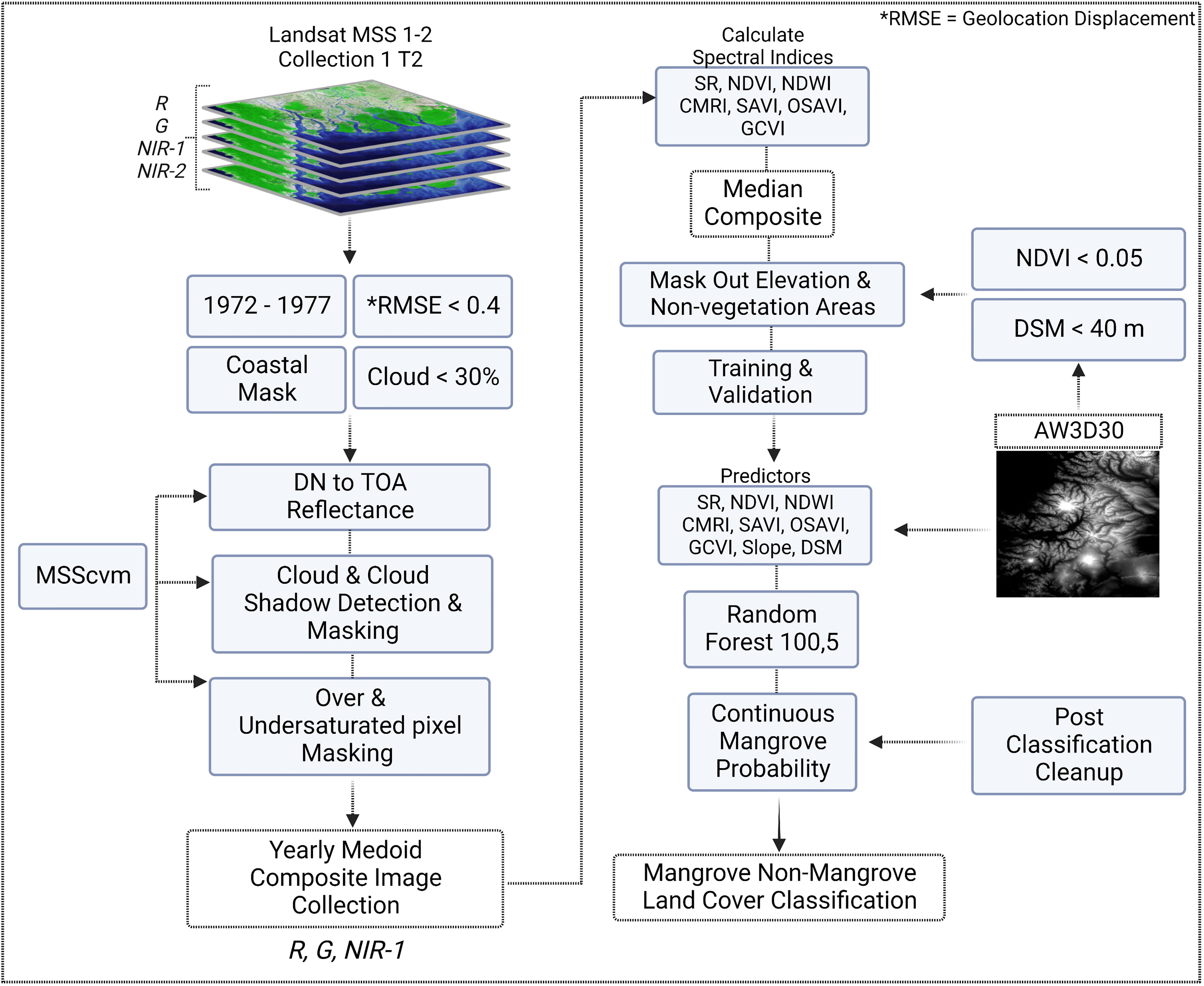
Figure 1 Overview of the methods used to conduct a random forest classification of mangrove forest extent in the case study countries. The analysis consisted of filtering and pre-processing; creation of yearly image composites; calculation of predictors; masking to constrain the analysis; a random forest classification; and post-classification cleanup.

FIGURE 2

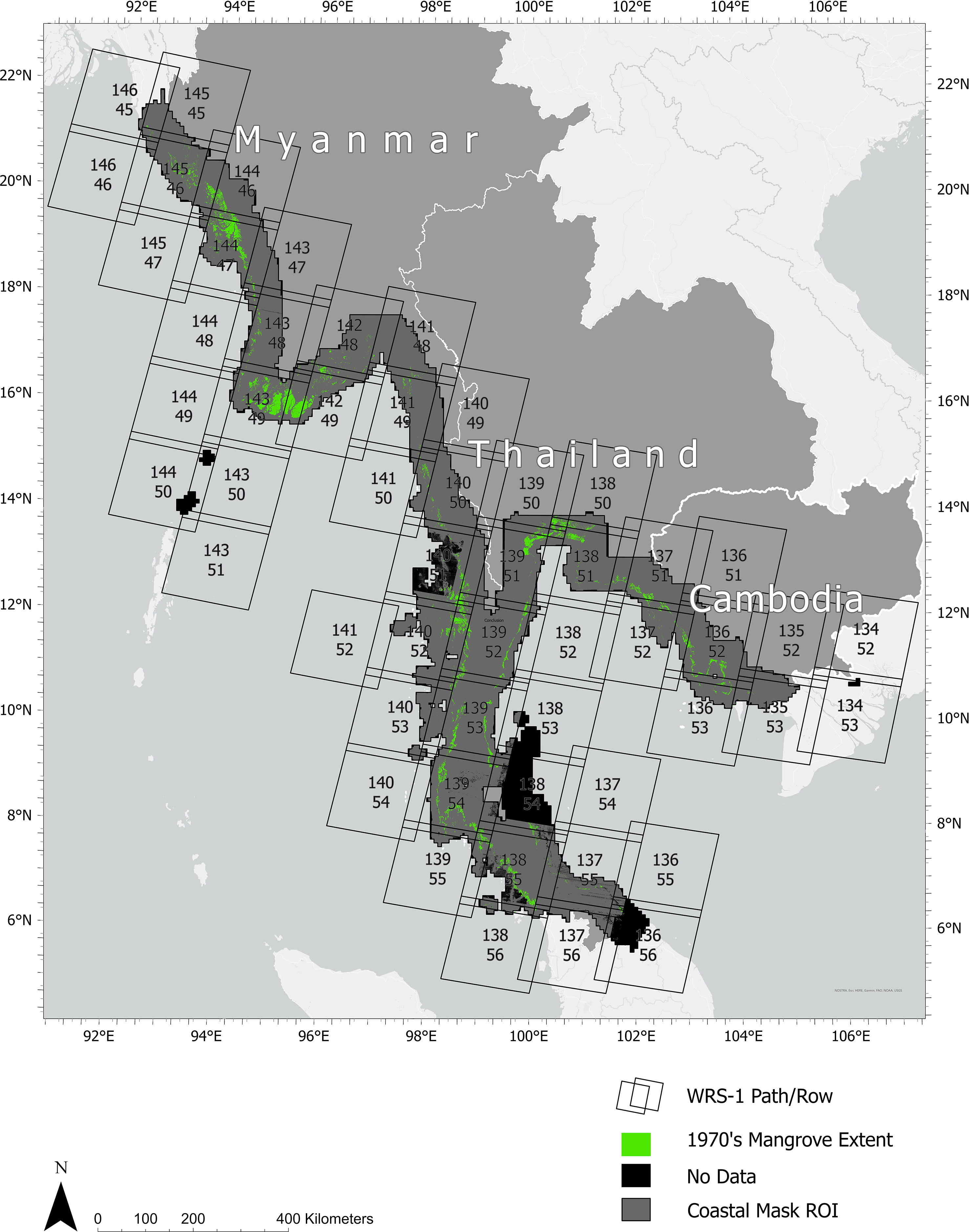
Figure 2 The study area showing the coastal mask that was generated to constrain the analysis to mangrove areas, the relevant WRS-1 Path/Row of the Landsat images used, the areas with no available Landsat data, and the 1970s mangrove distribution.

FIGURE 3

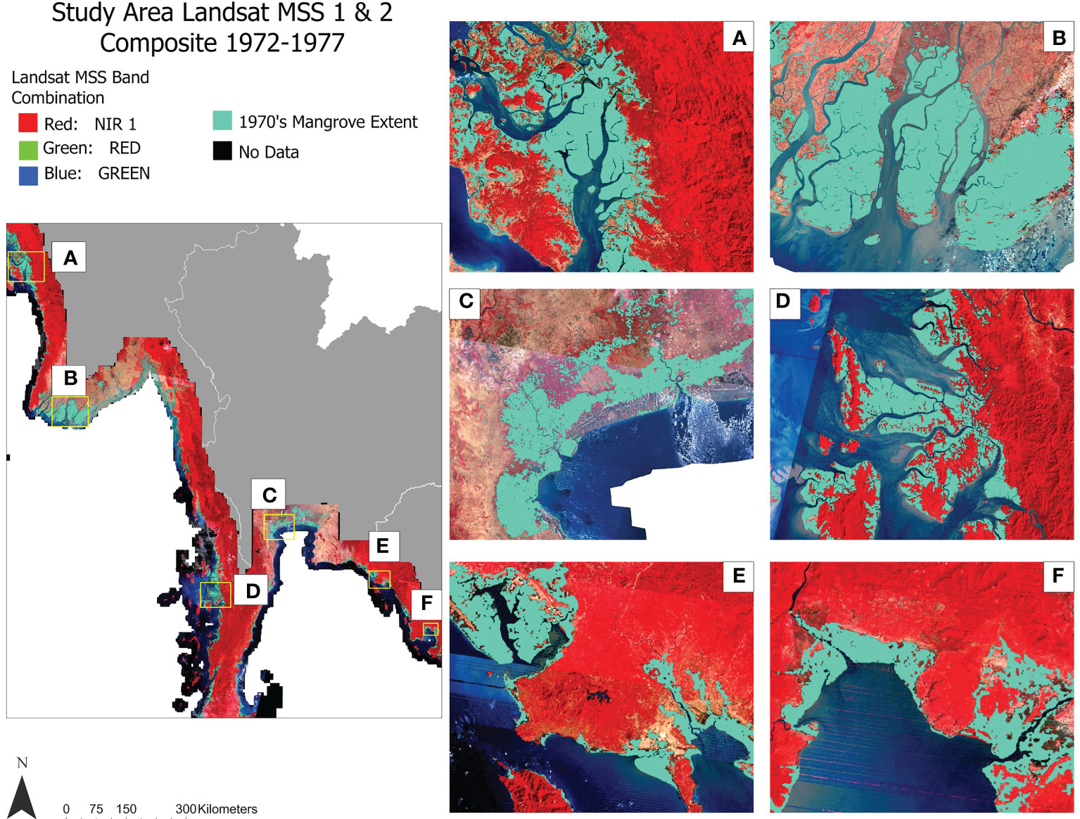
Figure 3 The LMSS composite circa 1972 to 1977. The displayed LMSS mosaic was constructed using the medoid on a yearly basis and then the yearly mosaics were composited using the median across the temporal period. The resulting random forest classification of mangrove extent is overlaid on the composite. Different mangroves across the study area are highlighted which include the (A) Rakhine state, Myanmar, (B) Ayeyarwady Delta, Myanmar, (C) Vicinity of Samut Sakorn, Thailand, (D) Tanintharyi Division, Myanmar, (E) Trat, Myanmar bordering Cambodia, and (F) Koh Kong Province, Cambodia.

Step one in our workflow included data filtering and selection followed by a series of pre-processing steps. To delineate coastal areas and subset the LMSS data needed for processing, a coastal mask was generated to include all potential mangrove areas. The mask included: the known extent of more current mangroves and coastal wetlands based on the global Wetland Extent Map (Mcowen et al., 2017) and the GMW dataset (Bunting et al., 2022), areas within 10 km of the shoreline, based on the global shorelines data (Sayre et al., 2019) and areas lower than 20 m elevations based on the Shuttle Radar Topography Mission (SRTM) DEM (Farr et al., 2007; Yang et al., 2011).

Given the unavailability of Tier 1 Landsat data, we utilized LMSS Tier 2 data for our analysis. Scenes with this level of processing have a lower radiometric and positional quality, but due to the lack of available scenes, this collection was selected. The coastal mask was used to select scenes from LMSS Tier 2, which were scaled and calibrated to at-sensor radiance. Only systematic terrain (L1GT) and systematic (L1GS) processing were applied to this collection due to insufficient ground control, excessive cloud cover, and geolocation issues (U.S. Geological Survey Department, 2018). This collection has a resampled spatial resolution of 60 m and a spectral range of 0.5–1.1µ including the Green, Red, NIR-1, and NIR-2 channels, and corresponds to WRS-1 (Wulder et al., 2022; U.S. Geological Survey Department, 2018). All scenes available from 1972 to 1977 were selected using the coastal mask as a spatial filter, which was then followed by a series of exclusionary steps. Scenes that did not have all of the five bands present which are the Red (B4), Green (B5), Near Infrared 1 (B6), Near Infrared 2 (B7), and the quality assurance bitmask (QA_Pixel) bands were excluded. Additionally, scenes were excluded if they had L1GS processing, exceeded a spatial displacement greater than ~24m or a root mean square value of 0.4, and cloud cover greater than 30%; effectively reducing imagery from 3,153 to 689 (see Figure 4). Images were then manually excluded if they had excessive cloud cover over mangrove areas, erroneously saturated pixels, or abnormal image artifacts, further reducing the collection to 371 images (see Figure 5). These issues were related to excessive detector striping, transcription artifacts, abnormal saturation, memory effect, and scan mirror pulse errors (U.S. Geological Survey Department, 2018; Vogeler et al., 2018).

FIGURE 4

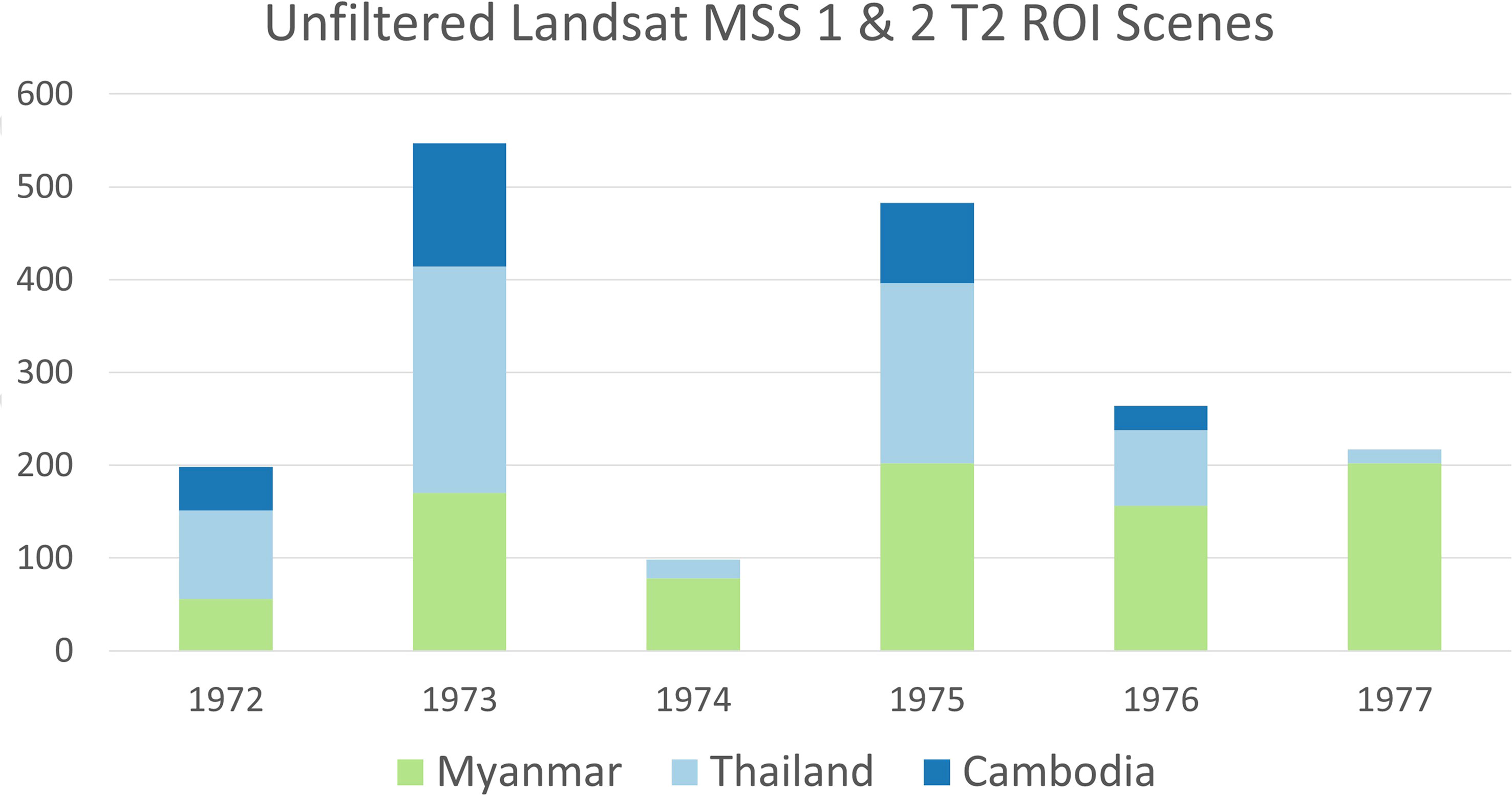
Figure 4 A histogram showing the image counts for all available Landsat 1 & 2 imagery over the region of interest and over the years of 1972 to 1977. The histogram shows that image availability was high before the filter process was initiated.

FIGURE 5

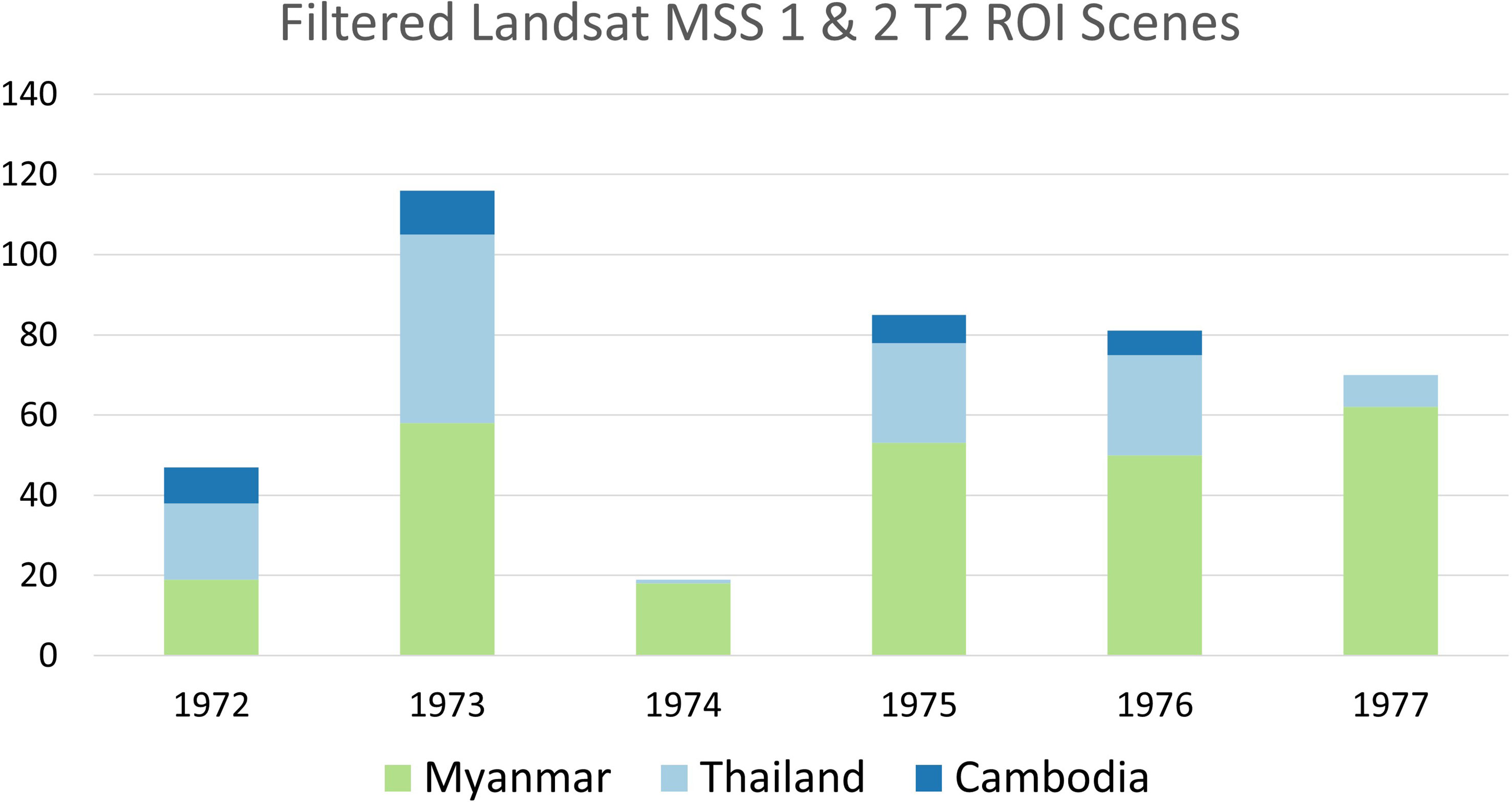
Figure 5 A histogram showing the image counts for all available Landsat 1 & 2 imagery over the region of interest and over the years of 1972 to 1977. Image availability was decreased by 88.23% once filters were applied to the collection to exclude imagery based on RMSE, cloud cover %, spatial characteristics, sensor attributes, and scene processing.

Following the manual inspection and removal of Landsat scenes from Landsat MSS over the study area, the next step was to mask out cloud cover and correct the imagery to top-of-atmosphere reflectance. We did this by using an automated cloud and cloud shadow detection and masking algorithm proposed by Braaten et al. (2015), called the Landsat Multispectral Scanner System clear-view-mask or MSScvm. This algorithm is an already established automated approach that identifies and masks out clouds based on green band brightness and the normalized difference between the green and red bands. It further identifies and masks cloud shadows using near infrared band darkness and cloud projection. Along with this cloud detection, it also corrects for topography-induced illumination and water identification using a digital elevation model (Braaten et al., 2015). Then on a per image basis, MSScvm was applied to each image effectively removing the majority of cloud cover and cloud shadow. Following that, we created a mosaic for subsequent classification. As shown in Figures 4, 5, the amount of imagery is highly variable. This study selected the years 1972 to 1977 due to these years having the highest and most semi-consistent image count with almost wall to wall coverage (see coastal mask in the Figure 1 study area) during the 1970s. Once the images were identified, the cloud free mosaics were generated per calendar year from 1972 to 1977 on a per pixel basis using the medoid, a more robust version of the median. Although these studies are more effective with seasonal composites, this was not feasible due to low image counts. The medoid represents the point with the minimal summed distance to all points in a data set. It also takes into consideration the multiple dimensions in the selection relevant to the different bands of a scene found within a year (Flood, 2013). The medoid was calculated by finding the difference between the median and the corresponding median of each band squared followed by finding the sum of the powered differences across bands per image for all observations. These annual medoid mosaics were much more sensitive to extreme outliers resulting in a more consistent representation of the study area. This approach was also selected to account for the inconsistent number of Landsat observations per year. The yearly medoid image collection was then used to produce a single five-year composite over the study period using the median across all medoid observations (see Figure 3 for composite results and Figure 1 for workflow).

Following the steps used to create a single mosaic of LMSS from 1972–1977, a series of indices were calculated that are ideal for mapping mangrove extents (Yancho et al., 2020). The indices that were calculated include the simple ratio (SR), normalized difference vegetation index (NDVI), the normalized difference water index (NDWI), the combined mangrove recognition index (CMRI), the soil-adjusted vegetation index (SAVI), the optimized soil-adjusted vegetation index (OSAVI), and the greenness chlorophyll vegetation index (GCVI) which serves as a proxy for chlorophyll content and proved to be useful in some mangrove mapping studies (Jordan, 1969; Tarpley et al., 1984; Huete, 1988; Gao, 1996; Gupta et al., 2018; Yancho et al., 2020; Rondeaux et al., 1996; Gitelson et al., 2003; Chamberlain et al., 2021). In addition to the vegetation indices, slope and elevation were also incorporated which was extracted from JAXA’s Land Observing Satellite (ALOS) (Takaku et al., 2014; Takaku et al., 2020). The predictors used for the random forest classifier can be referred to in Table 1 in addition to the original bands used in the LMSS collection.

TABLE 1

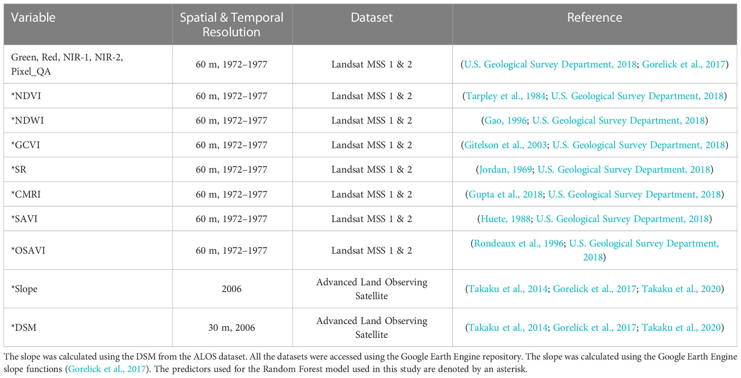
Table 1 The vegetation index inputs were created using the bands from Landsat MSS 1 & 2 as listed on the first row.

Before beginning the process of collecting model calibration and validation samples, masks were applied to the coastal region of interest (see Figure 1) using the ALOS DSM (Takaku et al., 2014; Takaku et al., 2020) and NDVI bands. These datasets were used to exclude areas that were not vegetation using NDVI pixels less than 0.05 and areas of elevation greater than 40 m. This masking excluded any area that did not have an NDVI values associated to dense vegetation, such as urban, water, and bare ground areas in addition to higher elevation areas. Given this level of masking, this study specifically focused on dense assemblages of mangrove forests and excluded only the most fragmented mangroves with low NDVI values. Training polygons were collected using the final composite by digitizing areas representing the most homogenous mangrove and non-mangrove vegetation pixels. Due to the lack of reference data from the 1970s, the composite itself was used as a reference to digitize the training samples. In total, 1,134 points were selected for the mangrove (n=283) and non-mangrove (n=851) land cover classes. Using the Landsat MSS composite (see Figure 3) an area was designated as mangrove if it was found within the coastal mask region, was found along the coastline, found along tributaries closest to the coastline, had a dense texture, and was a patch with high and consistent NDVI values. The non-mangrove training areas were selected based on whether it was found in water, areas at greater distances from the coast, and in groupings of pixels that were not homogenous or did not have a high NDVI value. These characteristics were chosen given that the minimum mapping unit (MMU) was around 0.16 ha and that we had a goal of mapping an assortment of mangrove trees and not individual mangrove trees below the MMU.

Following the preparation of predictors and collection of training samples, a random forest algorithm was used to predict the distribution of mangrove and non-mangrove areas for the entire study area using the LMSS mosaic. Random forest is an approach that uses non-parametric classification and decision trees in addition to classification and regression trees (Breiman, 2001). The hierarchy of this classifier is composed of a root node, inclusion of predictor samples, node separator with relevant decision rules, and the end of the leaf node with the desired classes – or in our case the probability of belonging to the mangrove class. Random forest was also chosen because models in other studies resulted in higher accuracies in comparison to other decision tree classifiers (Breiman, 2001; Pal, 2003; Ghimire et al., 2012; Belgiu and Drăguţ, 2016). The predictors that were selected for the model used in this study included the previously prepared indices or elevation parameters; SR, NDVI, NDWI, CMRI, SAVI, OSAVI, GCVI, and DSM. The random forest model we selected utilized a total of 100 trees sampled at random for every 5^th predictor, a minimum leaf population of 1, a bag fraction of 0.5 per tree, no limit on the maximum number of leaf nodes in each tree, a randomization seed value of 0, with the output mode set to a probability output. Following this classification of continuous mangrove probability, a series of post classification steps were used to remove noise and to threshold the classification’s bimodal distribution. First the classification was automatically thresholded using a gray level histogram detection method proposed by Otsu (1979) to divide the layer into two distinct classes, mangrove, and non-mangrove. Once the classification was automatically converted into a binary classification of mangrove and non-mangrove areas, the classification was cleaned up to remove noise using a majority filter. The majority filter was applied using a 3 by 3 kernel majority filter where a given pixel would be changed if most of the cells within a neighborhood were contiguous. Following the majority filter, a series of dilation and erosion techniques were used to generalize the zones using an evaluation of immediate orthogonal and diagonal neighbors for a given mangrove or non-mangrove region (Serra, 1982). The order of sorting priority was based on the size of the mangrove and non-mangrove zones when performing the classification smoothing. The classification was manually cleaned up to eliminate additional salt and pepper areas, areas that had visible errors introduced by excessive cloud cover or had any additional noise. An example of this would be any errors of commission found farther from the coastline where brackish waters are less concentrated.

To assess the classification, we followed the “good practices” proposed by Olofsson et al. (2013) and Olofsson et al. (2014) using a random stratification approach over the study area. It is important to note that the area proportion for the mangrove and non-mangrove class were 16% and 84% of the total study area and the sample allocation was based on the smaller area proportion class (mangrove). Furthermore, we anticipated an accuracy of 70% and a proportion of 20% for the mangrove class, and a target standard error of 1%. This leveraged a set of 300 samples for the non-mangrove class and a set of 67 samples for the mangrove class. However, a total of 28 were impossible to verify visually, therefore our final dataset resulted in 339 samples: 54 to mangrove and 285 to non-mangrove. The verification process took place in the Collect Earth platform (Bey et al., 2016; Saah et al., 2019), each sample was inspected using both the original LMSS mosaic, Google Earth Imagery (Lisle, 2006), and the classification overlaid as a reference. Sample points were validated as mangrove when 50% of a 30 m x 30 m square centered about a sample point had a higher NDVI reflectance (manifested as a dark red color), were adjacent to the coastline, at the intersection of a river outlet and the ocean, or were greater than the MMU of ~0.16 ha. The non-mangrove class was labeled if a given sample point was found in open water, bare ground with some vegetation cover, water with some vegetation, heavily fragmented vegetation, and vegetation that was not immediately adjacent to the coastline or river outlets for greater than 50% of a 30 m x 30 m area. Then the attribute table of the validation point was updated by extracting the value found in the classification at each point location. This was used to calculate the error matrices, overall, producer’s, user’s accuracy, and Kappa Coefficient.

Once the classification and accuracy assessment was completed, we analyzed the extent of mangrove ecosystems for our ROI within the context of each country’s unique circumstances, GMW extents, and other external estimates. In order to measure change in mangrove extent between the 1970s and 2020, we compared our 1970s mangrove cover map to maps created by GMW for 1996, 2007, 2010, 2016, and 2020 (Bunting et al., 2022). The GMW maps were reprojected and resampled to match the spatial resolution of the LMSS classification results. Then, the layer was rasterized. Lastly, the GMW raster was masked to exclude all areas that overlapped with no Landsat observations available in the final LMSS classification product.

3 Results

3.1 Data processing and uncertainty

A total of 3,153 images were identified during the initial data exploration phase before additional filters were applied. This study identified 371 images suitable for classification that met spatial offset and cloud cover filters, which reduced the available imagery by 88%. The study had an average of 63 ± 38 images per year but with significant interannual variability. The highest image availability occurred in 1973 (n = 109) and 1976 (n = 103). The year with the lowest image count was 1974 with 9 images. Following the filtering and scene selection phase, the LMSS imagery was corrected to top-of-atmosphere, cloud and cloud shadow masked, and then composited into a mosaic over the study period resulting in a cloud free medoid mosaic of LMSS. This approach likely has high amounts of variability and uncertainty due to the lack of observations & the inability to map mangrove cover seasonally. Additionally, the coarser spatial, spectral, and radiometric resolution of MSS constrains the capacity for mapping mangroves during the 1970s. This work would greatly benefit from additional efforts to map mangroves on a seasonal basis over a longer time period consistently with harmonization across all of Landsat’s sensors as done by other studies (Braaten et al., 2015; Zhu et al., 2018; H. Nguyen et al., 2019; Yan and Roy, 2021). Following the classification, the final mangrove data product was assessed for accuracy, but with other constraints.

The overall accuracy and kappa coefficient was 95% and 0.82 respectively. Producer’s and User’s accuracy were 98% and 96% for the non-mangrove class and 80% and 90% for the mangrove class (Table 2). These accuracy results indicated that the model was less likely to identify real mangrove features on the ground in comparison to the mapped mangrove feature in the map. The higher reliability, or User’s accuracy for the mangrove class indicated that map users were more likely to find the mangrove areas identified in the map on the ground. Some of these uncertainties were likely related to the quality of the mosaic and how consistent a given pixel may be. Take for example the issue of low image counts for 1974 in this study and the fact that there were regions with no Landsat observations.

TABLE 2

Table 2 Accuracy metrics.

3.2 1970s baseline of mangrove extent and assessment of change from 1970s to 2020

Our 1970s map of mangrove extent identified 15,420 km² across our study area (Table 3). Myanmar had the greatest extent of mangroves (9,272 km²), followed by Thailand (5,407 km²) and Cambodia (742 km²). When comparing our new 1970s baseline data to existing GMW maps of mangrove extent, we found a sharp decline in mangrove area between the 1970s and 1996. Across the study region, mangrove area declined by 47% (corresponding to a loss of 8,239 km²) during this period (Table 3). Loss rates were highest in Thailand (58%) and lowest in Cambodia (14%). In Thailand, declines in mangrove areas were especially pronounced around Bangkok and along the eastern portion of the Gulf of Thailand (Figure 6). In contrast, areas with the greatest occurrence of persistence and gain were found in the Mu Ko Phayam National Park along the coastline up to the Mu Ko Ra-Ko Phra Thong National Park. Myanmar experienced a 42% decline in mangrove area between the 1970s and 1996. Here, loss was greatest around the Ayeyarwady Delta (Figure 7). In Cambodia, most losses were concentrated along the Koh Kong coastline in the northwestern portion of the country (Figure 8). Although Cambodia experienced overall declines in mangrove extent between 1970s and 1996, there were some southwest gains in the Bay of Kampong Som in the Botum Sakor District of Koh Kong Province (Figure 8).

TABLE 3

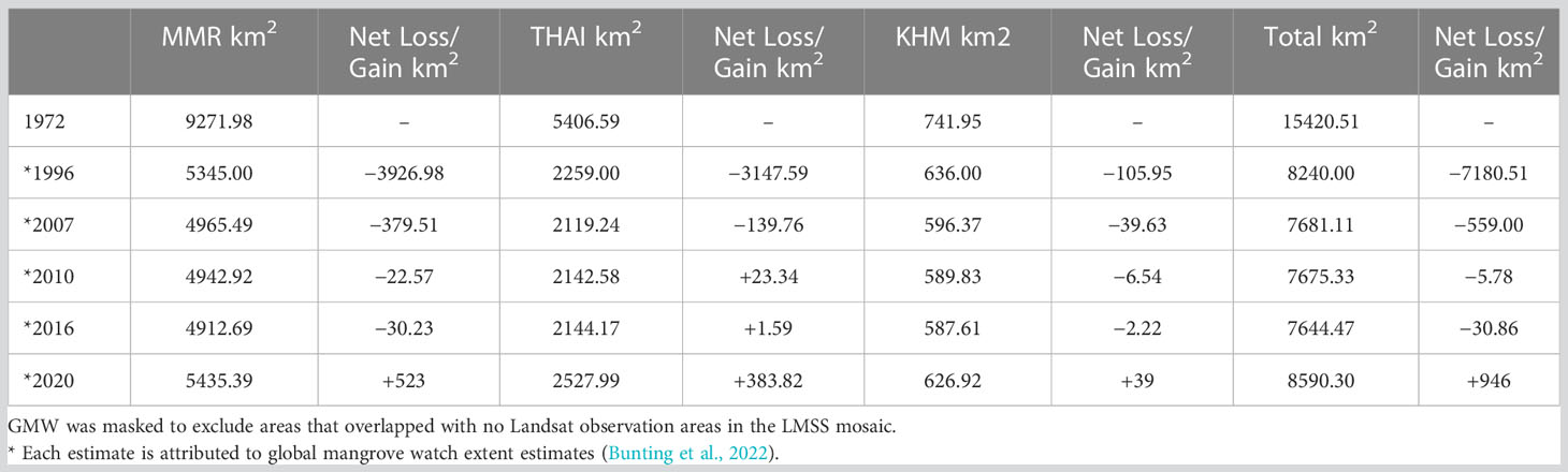
Table 3 A comparison of extent estimates from the new 1970s baseline and the *GMW extent.

FIGURE 6

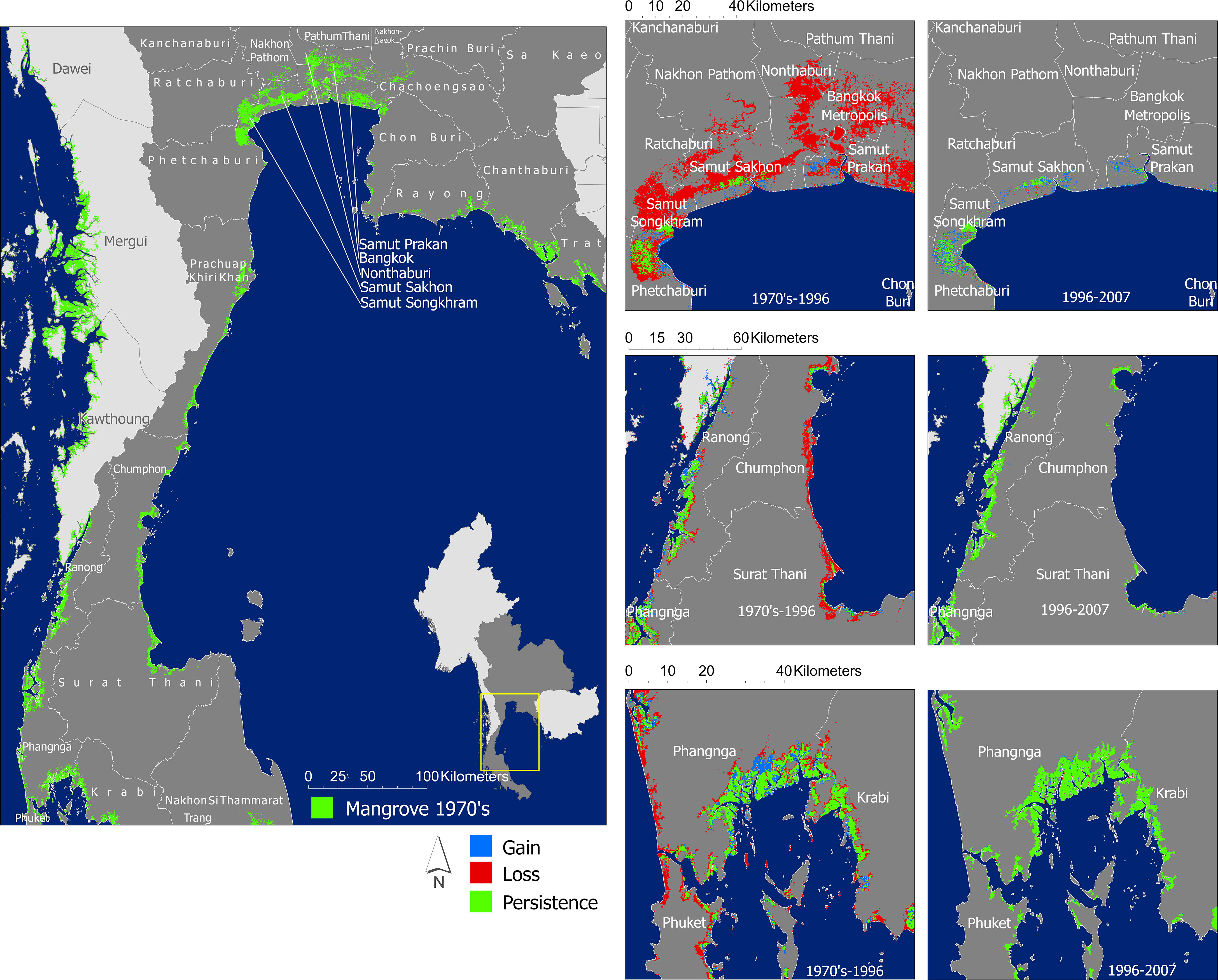
Figure 6 The classification difference between the 1970s Thailand mangrove baseline and the 1996 GMW mangrove extent. The losses were most significant in the Samut Sakhon, Nonthaburi, Bangkok, and Samut Prakan.

FIGURE 7

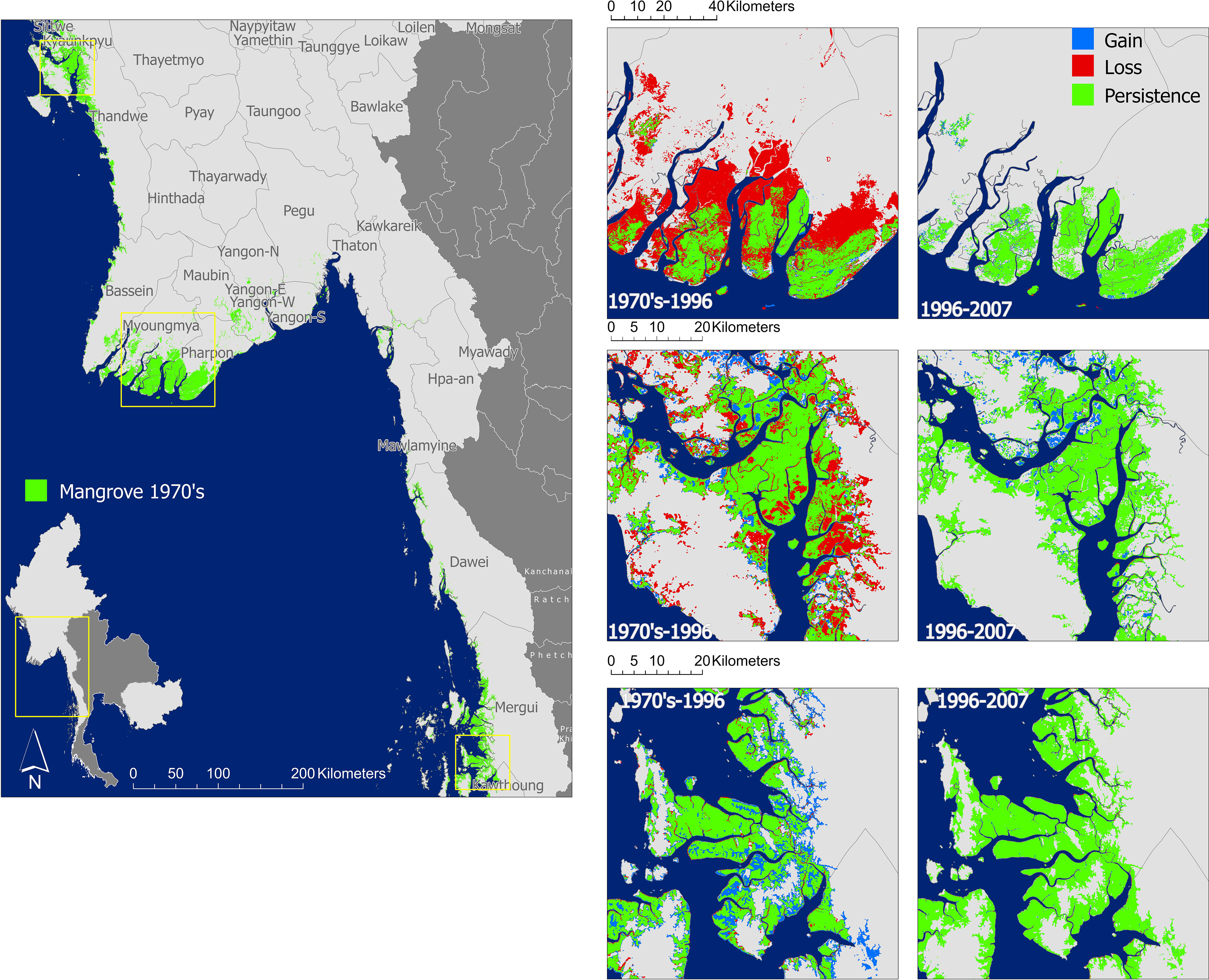
Figure 7 The classification difference between the 1970s Myanmar mangrove baseline and the 1996 GMW mangrove extent. The area of Myoungmya and Pharon showed the most jarring losses in Myanmar.

FIGURE 8

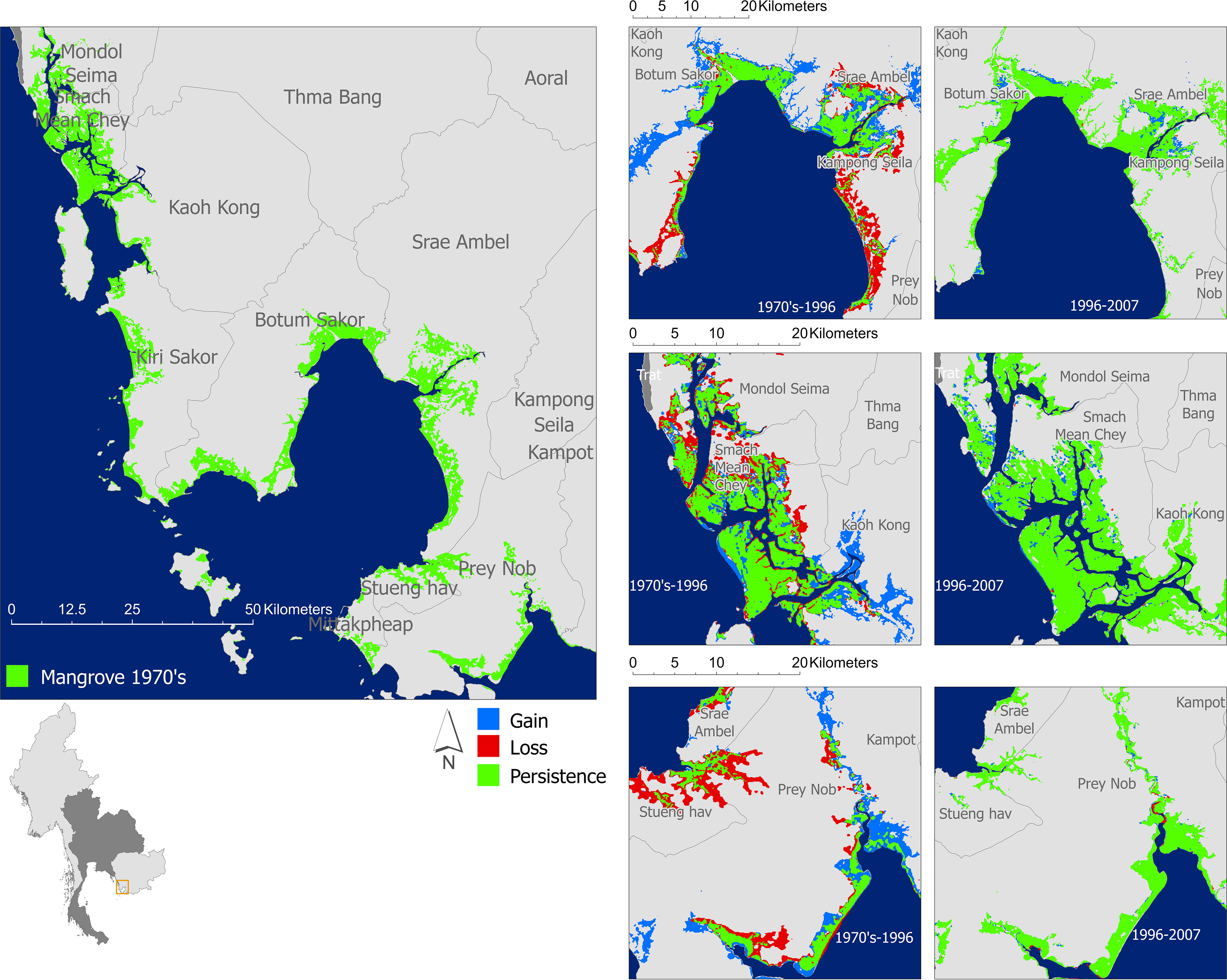
Figure 8 The classification difference between the 1970s Cambodia mangrove baseline and the 1996 GMW mangrove extent. The areas of Botum Sakor showed a trend of persistence, while Srae Ambel showed areas of mostly loss.

Firstly, the GMW estimates were masked using the areas labeled as 0 due to a lack of Landsat observations in the LMSS mosaic. The inventory of extent of different time points up to 2020 show that rates of mangrove loss across our study region declined dramatically after 1996 (Table 3; Figure 9). Overall, mangrove extent declined by 7% between 1996 and 2007 and these rates were similar across the three countries. Mangrove extent then showed little change between 2007 and 2016. Between 2016 and 2020, mangrove extent increased in all three countries; rates of mangrove expansion ranged from 7% (Cambodia) to 18% (Thailand). These results further extend our understanding of mangrove change before the 1990s, a period of data scarcity when it comes to mangrove data products.

FIGURE 9

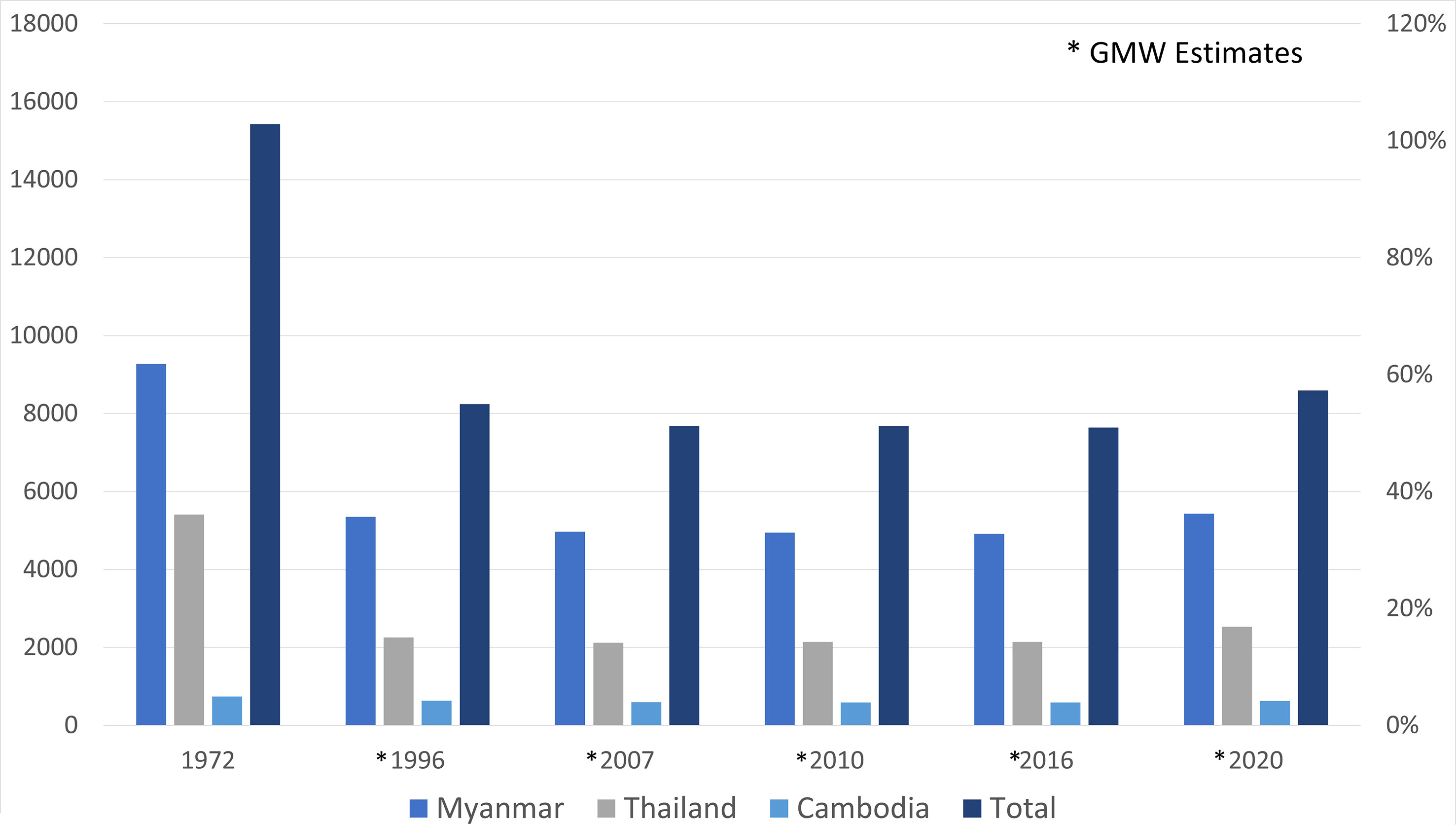
Figure 9 A histogram showing the distribution of mangrove extents comparing the new 1970s era baseline to the estimates for GMW at different time points; 1996, 2007, 2010, 2016, 2020. These estimates indicated an average loss of 44% from the 1970s to 2020 over the study period.

4 Discussion

4.1 Data processing challenges and limitations

In this study, we provided a semi-automatic approach to delineating the extent of mangrove area using LMSS data from the 1970s. We leverage the earliest available Landsat imagery using MSS and compared it to more recent mangrove extent maps to understand historical mangrove change. However, some limitations remain, for instance none of the LMSS data from this period has been processed to the highest level of terrain and precision (Braaten et al., 2015; Roy et al., 2016). The issues that affected the quality of the collection, a sensor that makes up a significant portion of the early Landsat record (Yan and Roy, 2021), were related to a variety of anomalous errors such as memory, effect, scan correlated shifts, and scan mirror pulse¹ . In addition to sensor-related issues, there is also the difficulty of conducting a remote sensing investigation in the case study countries, one of the planet’s cloudiest regions (Kontgis et al., 2015; Li et al., 2018; Oliphant et al., 2019). Because of these challenges, this study excluded imagery that had a spatial offset greater than 24 m, cloud cover of less than 30%, imagery with oversaturated pixels, or excessive striping. It should also be noted that the number of images found per year was not consistently the same (Figures 4, 5) or of an ideal quantity to do annual image classifications and change detection. As a result, we had to composite multiple years’ worth of data to cover the entire study area. These challenges will make it difficult to expand this approach to other countries outside of our study area.

Following this phase, careful measures were taken to identify the LMSS scenes that would be used in this study. The images then had to be preprocessed to TOA and cloud masked using the MSScvm (Braaten et al., 2015) algorithm. This algorithm was developed by researchers to overcome the challenge of automatically detecting and masking clouds from MSS (Braaten et al., 2015), but with some limitations. This algorithm was designed to work with temperate ecosystems, but due to the lack of automatic algorithms for MSS cloud detection, MSScvm was selected for pre-processing procedures. Many measures were taken to identify the best approach to establishing a new baseline, but these limitations must be considered.

4.2 Shifting perspectives on mangrove change

With our new 1970s baseline map of mangrove extent in our case study countries, we identified a sharp decline in mangrove extent primarily for Myanmar and Thailand between the 1970s and 1996. However, after 1996, mangrove loss rates declined dramatically, and mangrove extent has been relatively stable since the mid-2000s according to this assessment. We do believe that an additional effort must be done to map the extents more consistently and harmoniously across sensors over a dense time series. But that was not possible at this time because of the lack of MSS scenes of sufficient quality. The proximate and underlying drivers of gains and losses for our study area are complex due to the history of political and economic instability from situations like the reign of the Communist Party of Kampuchea (CPK) over the course of 1975 to 1979 in Cambodia (Mosyakov, 2000) or the lack of electricity and subsequent need for mangrove firewood (from the Ayeyarwady delta) in the Yangon province of Myanmar. Furthermore, studies have indicated that some of the Myanmar and Cambodia mangrove losses may have been attributed to Thailand’s ban on logging in 1989 (Brown et al., 2001) proving that conservation measures can have unintended deforestation consequences (Brown et al., 2001; Pumijumnong, 2014; Lim et al., 2017). Meanwhile, Cambodia’s decades of political conflict under the reign of CPK may have resulted in lower rates of deforestation due to the lack of timber demand prior to the 1980s (Boutros-Ghali, 1994; Le Billon, 2000). Studies on the political ecology coupled with this study can help shed light on the transition from war to peace or the nature of different industries and their impacts on land cover and land use change.

4.3 Country specific perspectives

In Cambodia, we calculated a total of 742 km² for the period of 1972 to 1977. This is a more conservative estimate compared to other studies that inventoried a total of 946 km² for the same period without using remote sensing (Cambodia Land Cover Atlas 1985/87–1992/93, 1994; Cambodia Forestry Policy Assessment, 1996; Ministry of Environment, Kingdom of Cambodia, 2009). Following this time period, one study estimated a total of 758 km² for 1989, while another study mapped a total of 646 km² by 1996 (Kozhikkodan Veettil and Quang, 2019; Bunting et al., 2022). Over the course of 1996 to 2016, different studies estimated a mangrove loss of 208–300 km². When comparing the new 1970s baseline to the estimate by Bunting et al. (2022) in 2020, this study indicates an additional loss of 115 km² ± 174 km². Many of the drivers of degradation and change have been attributed to shrimp pond aquaculture; salt pan and charcoal production; and infrastructure development (Kozhikkodan Veettil and Quang, 2019), but we suggest that the drivers of change were also very much political especially during the temporal period of this study (Boutros-Ghali, 1994; Le Billon, 2000).

It is important to note that several studies have indicated a high level of uncertainty on Cambodian mangrove forest estimates (Rizvi and Singer, 2016; Nop et al., 2017; Kozhikkodan Veettil and Quang, 2019). Although there is some uncertainty, these statistics show a trend of little change between the 1970s era up to 1996 and may serve as additional support to other claims on the political drivers of mangrove persistence. During the period of 1975 to 1979, the CPK (Boutros-Ghali, 1994; Le Billon, 2000) was the ruling regime in Cambodia. During this time, the country experienced severe famine, deaths associated to the lack of medicine, the proliferation of disease, and mass genocide which led to the deaths of up to 1.5 to 2 million people (Locard, 2005). These extremely difficult circumstances indirectly enabled forest stability and even gains (Le Billon, 2000) throughout the 1970s, which helped almost two-thirds of the country to be completely forested by the early 1980s (Cambodia Land Cover Atlas 1985/87–1992/93, 1994). Also, the aquaculture industry was not actively introduced until 1960 in Cambodia and was relatively inactive during the time of the CPK conflict. The active political conflict coupled with the lack of aquaculture activities are the likely drivers of mangrove stability seen between the 1970s to the 1990s.

Our estimate of mangrove extent from the 1970s for Thailand (5,407 km²) were somewhat higher than estimates from previous studies that mapped an extent with a range of 3,127–3,679 km² (Aksornkoae, 2012; Pumijumnong, 2014; Charupphat and Charupphat, 1997; Klankamsorn and Charuppat, 1982; Barbier and Cox, 2002; Naito and Traesupap, 2014). However, the large losses in mangrove extent that we observed between the 1970s and 1996 agree with other studies (Charupphat and Charupphat, 1997; Klankamsorn and Charuppat, 1982; Aksornkoae, 2012; Naito and Traesupap, 2014). One such study that documented the economic and demographic drivers of mangrove losses over the course of 1975 to 1996 in Thailand indicated that almost half (46%) of all mangroves were lost to coastal shrimp farming (50–65%) and the increased demand for land in coastal areas due to urbanization and agriculture during the period of 1979 to 1996 (Barbier and Cox, 2002; Spalding et al., 2010). This study indicates that the losses were 12% greater (58%) over the same time.

Mangrove losses associated with Thailand were primarily related to the demand for land development, aquaculture, economic incentives, and policy failures, but only up until industries started to aggressively expand. The studies by Barbier and Cox (2002) and Bantoon (1994) observed how even though aquaculture was introduced as early as 1974, the industry began to have severe mangrove loss impacts after 1985 due to Japanese demand (Bantoon, 1994; Barbier and Cox, 2002). In addition, sustained economic growth caused coastal populations to grow, boosting the demand for urbanization and economic crowding around mangrove areas. This caused shrimp production to go from 15,000 metric tonnes (KMT) in 1985 to 264,000 KMT in 1994 (Pednekar, 1998; Barbier and Cox, 2002). It also caused the shrimp farm area to rapidly expand between 1983 and 1996 and the number of farms to increase from 3,779 to 21,917. This boom in the aquaculture industry in addition to increased urbanization are the likely contributors to the severe mangrove losses seen throughout Thailand.

Previous estimates of mangrove extent and change in Myanmar exhibit a large amount of variation, highlighting the need for better data for this region (Aung, 2007; Spalding et al., 2010; Thant et al., 2012; Webb et al., 2014; Giardino et al., 2016; Veettil et al., 2018; Alban et al., 2020). Some of these claims documented that extreme overexploitation began as early as the Second World War to satisfy the demands of the military with the worst forest overexploitation occurring over the period of 1949 to 1972. According to Oo (2002) and Kyi (1992), mangrove forests in the Ayeyarwady delta decreased from 2,345 km² in 1954 to 1,786 km² in 1984. This study speculated losses that are much higher than our findings which established an area of 9,272 km² in the 1970s. More recently, Bunting et al. (2022) mapped a total of 5,821 km² of mangroves across the entire country in 1996, while Alban et al. (2020) mapped a total of 13,233 km² for the same year. These contradictory statistics demonstrate the need for region-specific mapping approaches in lieu of sub-setting a global dataset to report on country specific mangrove extent (Estoque et al., 2018; Alban et al., 2020). Also, Alban et al. (2020) estimated higher rates of mangrove deforestation in Myanmar, with 60% of mangroves permanently or temporarily lost between 1996 and 2016 due to the cultivation of rice, oil palm, and rubber in addition to urbanization.

Other studies that were done during the 1990s indicated additional land use drivers of change were to blame for the severe losses that were also found in Myanmar in the three main mangrove regions: Ayeyarwady, Tanintharyi, and Rakhine. According to Oo (2002), the main objective of mangrove management was fuel-wood and charcoal production. Then during Myanmar’s period of insurgency (1949–1972), the forest department was not able to effectively use forest management at large. However, mangrove species were not as affected by commercial demand, but by local demand. For example, the more heavily populated area of Yangon relied heavily on mangrove for charcoal and firewood production from the Ayeyarwady area, resulting in heavy losses. The Rakhine state on the other hand is an area with lower population and was speculated to have minimized losses according to Oo (2002) in the early 2000s. Higher populations and the demand for charcoal and fuel wood production therefore led to more extensive mangrove losses according to these studies. Following such losses, the Forest Department started intensive mangrove planting projects in 1975 followed by strict prohibitions of mangrove-derived charcoal and firewood after 1993. An important distinction that the study by Oo (2002) made is that many of the areas were experiencing losses due to the lack of electricity and need for energy which was an indirect driver of the fuel wood and charcoal production industry before prohibition.

Much of the losses of mangroves in our study region were driven by economic concerns. The Ayeyarwady delta of Myanmar experienced losses to mangrove charcoal and firewood production, but this resource was used to address the complete lack of electricity in the adjacent area of Yangon. This study indicated that almost half of mangrove area was lost by 1996, but we also urge researchers to have a sensitive perspective on the drivers behind the loss. Yes, these losses were extensive, but these results should be considered within the context of the people of Myanmar who had an urgent need to address their energy security, or the coastal communities of Thailand who pursued the economic benefits of the shrimp industry or urbanization, and the people of Cambodia who worked diligently towards reconstruction after the Khmer rouge. This study allowed us to not only establish a new baseline that would better inform current understandings of mangrove change before the 1990s, but it aided our understanding of the different needs that the people and their governments were trying to meet. We hope that this new baseline and conversation on the political ecology can serve as an example of good research practices in trying to understand mangrove change dynamics without forgetting about the human element.

5 Conclusion

Myanmar, Thailand, and Cambodia are home to one of the planet’s most biologically complex and carbon rich mangrove ecosystems. There is a high degree of variability in the cadence and severity of mangrove change in these complex coastal ecosystems. Ultimately, the social and ecological values of these mangrove ecosystems have urged a sustained effort to produce a variety of region and sub-regional mangrove extent data products and inventories for this area. However, mangrove extent and change dynamics before the mid-1990s are not well constrained and this area is no exception. Due to the limited availability of publicly available EO data of sufficient quality or availability, conducting a remote sensing analysis of this nature is supremely difficult. This study therefore worked to identify a semi-automatic approach to quantify mangrove distribution over the course of 1972 to 1977 using the best available Landsat 1-2 MSS Tier 2 data. The extent maps in this study were generated using a Random Forest model that mapped a new baseline extent of 15,421 km² with a resulting overall accuracy of 95%. The accuracy assessments also indicated a producer’s accuracy of 80% and 98% and a user’s accuracy of 90% and 96% for the mangrove and non-mangrove class. The study further established historical losses by comparing the new baseline to external mangrove estimates from GMW. This comparison indicated that mangroves were reduced by 6,830 km² (44%) by the year 2020. The majority of mangrove losses therefore occurred between the 1970s and the 1990s followed by an immediate trend in mangrove persistence. This study also elaborated on the political, social, and economic drivers of change for this area and urge the remote sensing community to do the same.

Data availability statement

The raw data supporting the conclusions of this article will be made available by the authors, without undue reservation.

Author contributions

Conceptualization, PB, PM-S, KC, CD, DL, MS, and TF; methodology, PB, CD, PM-S, and TF; validation, PB, PM-S, and CD; formal analysis, PB, PM-S, and CD; data curation, PB, PM-S, and CD; writing—original draft preparation, PB, PM-S, KC, and CD; writing—review and editing, PB, PM-S, KC, CD, DL, TT, MS, and TF; visualization, PB; supervision and project administration, KC, MS, and TF; funding acquisition, KC, DL, MS, and TF. All authors contributed to the article and approved the submitted version.

Funding

All authors were funded by NASA’s Land Cover and Land Use Change (LCLUC) Project: “Global Hotspots of Change in Mangrove Forests Project”, award number 2020 20-LCLUC2020-0050. Part of this work was performed at the Jet Propulsion Laboratory under contract with the National Aeronautics and Space Administration (NASA).

Acknowledgments

We would like to express our gratitude to folks who helped contribute ideas during the entirety of the project. We would also like to give a special thanks to all the authors who remained committed despite the challenges of an ongoing pandemic or challenges with health.

Conflict of interest

The authors declare that the research was conducted in the absence of any commercial or financial relationships that could be construed as a potential conflict of interest.

Publisher’s note

All claims expressed in this article are solely those of the authors and do not necessarily represent those of their affiliated organizations, or those of the publisher, the editors and the reviewers. Any product that may be evaluated in this article, or claim that may be made by its manufacturer, is not guaranteed or endorsed by the publisher.

Footnotes

1. ^ https://www.usgs.gov/landsat-missions/landsat-known-issues

References

Adame M. F., Connolly R. M., Turschwell M. P., Lovelock C. E., Fatoyinbo T., Lagomasino D., et al. (2021). “Future carbon emissions from global mangrove forest loss. Glob. Chang. Biol. 27 (12), 2856–2866. doi: 10.1111/gcb.15571

PubMed Abstract | CrossRef Full Text | Google Scholar

Aksornkoae S. (2012). Mangroves… coastal treasure of Thailand. J. R. Institute Thailand 4, 59–77. Available at: https://www.thaiscience.info/Journals/Article/TJRI/10990648.pdf.

Google Scholar

Alban J. D. T. D., Jamaludin J., de Wen D. W., Than M. M., Webb E. L. (2020). Improved estimates of mangrove cover and change reveal catastrophic deforestation in Myanmar. Environ. Res. Lett. 15 (3), 0340345. doi: 10.1088/1748-9326/ab666d

CrossRef Full Text | Google Scholar

Alongi D. M. (2014). Carbon cycling and storage in mangrove forests. Annu. Rev. Mar. Sci. 6, 195–219. doi: 10.1146/annurev-marine-010213-135020

CrossRef Full Text | Google Scholar

Aung U.M. (2007). Policy and practice in myanmar’s protected area system. J. Environ. Manage. 84 (2), 188–2035. doi: 10.1016/j.jenvman.2006.05.016

PubMed Abstract | CrossRef Full Text | Google Scholar

Bantoon S. (1994). Using simulation modelling and remote sensing technique for impact study of shrimp farms on mangrove area and aquatic animal production at welu estuary, khlung district, chantaburi province (Bangkok: Chulalongkorn University). Unpublished MSc Thesis.

Google Scholar

Barbier E., Cox M. (2002). Economic and demographic factors affecting mangrove loss in the coastal provinces of Thailand 1979-1996. Ambio 31 (4), 351–575. doi: 10.1579/0044-7447-31.4.351

PubMed Abstract | CrossRef Full Text | Google Scholar

Belgiu M., Drăguţ L. (2016). Random forest in remote sensing: a review of applications and future directions. ISPRS J. Photogrammetry Remote Sens. 114, 24–31. doi: 10.1016/j.isprsjprs.2016.01.011

CrossRef Full Text | Google Scholar

Bey A., Sánchez-Paus Díaz A., Maniatis D., Marchi G., Mollicone D., Ricci S., et al. (2016). Collect earth: land use and land cover assessment through augmented visual interpretation. Remote Sens. 8 (10), 807. doi: 10.3390/rs8100807

CrossRef Full Text | Google Scholar

Bouillon S., Borges A. V., Castañeda-Moya E., Diele K., Dittmar T., Duke N. C., et al. (2008). Mangrove production and carbon sinks: a revision of global budget estimates. Global Biogeochem. Cycles 22 (2), 207. doi: 10.1029/2007GB003052

CrossRef Full Text | Google Scholar

Boutros-Ghali B. (1994). Building peace and development: 1994 report on the work of the organization from the forty-eighth to the forty-ninth session of the general assembly (New York: United Nations Publications).

Google Scholar

Braaten J. D., Cohen W. B., Yang Z. (2015). Automated cloud and cloud shadow identification in landsat MSS imagery for temperate ecosystems. Remote Sens. Environ. 169 (November), 128–138. doi: 10.1016/j.rse.2015.08.006

CrossRef Full Text | Google Scholar

Brander L. M., Wagtendonk A. J., Hussain S. S., McVittie A., Verburg P. H., de Groot R. S., et al. (2012). Ecosystem service values for mangroves in southeast Asia: a meta-analysis and value transfer application. Ecosys. Serv. 1 (1), 62–695. doi: 10.1016/j.ecoser.2012.06.003

CrossRef Full Text | Google Scholar

Breiman L. (2001). Random forests. Mach. Learn. 45 (1), 5–32. doi: 10.1023/A:1010933404324

CrossRef Full Text | Google Scholar

Brown C., Durst P. B., Enters T. (2001). Forests out of bounds: impacts and effectiveness of logging bans in natural forests in Asia-pacific. (Bangkok, Thailand: FAO Regional office for Asia and the Pacific).

Google Scholar

Bunting P., Rosenqvist A., Hilarides L., Lucas R. M., Thomas N., Tadono T., et al. (2022). Global mangrove extent change 1996–2020: global mangrove watch version 3.0. Remote Sens. 14 (15), 36575. doi: 10.3390/rs14153657

CrossRef Full Text | Google Scholar

Cambodia Forestry Policy Assessment (1996). World Bank, United Nations Development Programme, and Food And Agriculture and Organization.

Google Scholar

Cambodia Land Cover Atlas 1985/87–1992/93 (1994). Rome, Italy: Food and agriculture organization.

Google Scholar

Chakraborty S., Sahoo S., Majumdar D., Saha S., Roy S. (2019). Future mangrove suitability assessment of Andaman to strengthen sustainable development. J. Cleaner Product. 234 (October), 597–614. doi: 10.1016/j.jclepro.2019.06.257

CrossRef Full Text | Google Scholar

Chamberlain D. A., Phinn S. R., Possingham H. P. (2021). Mangrove forest cover and phenology with landsat dense time series in central Queensland, Australia. Remote Sens. 13 (15), 30325. doi: 10.3390/rs13153032

CrossRef Full Text | Google Scholar

Charupphat T., Charupphat C. (1997) Application of landsat-5 (TM) for monitoring the changes of mangrove forest area in Thailand. Available at: https://scholar.google.com/scholar_lookup?title=Application+of+Landsat-5+%28TM%29+for+monitoring+the+changes+of+mangrove+forest+area+in+Thailand&author=Thongchai+Charupphat&publication_year=1997.

Google Scholar

Dahdouh-Guebas F., Cannicci S. (2021). Mangrove restoration under shifted baselines and future uncertainty. Front. Mar. Sci. 8. doi: 10.3389/fmars.2021.799543

CrossRef Full Text | Google Scholar

DeFries R. S., Rudel T., Uriarte M., Hansen M. (2010). Deforestation driven by urban population growth and agricultural trade in the twenty-first century. Nat. Geosci. 3 (3), 178–815. doi: 10.1038/ngeo756

CrossRef Full Text | Google Scholar

Devaraj C., Shah C. A. (2014). Automated geometric correction of landsat MSS L1G imagery. IEEE Geosci. Remote Sens. Lett. 11 (1), 347–515. doi: 10.1109/LGRS.2013.2257677

CrossRef Full Text | Google Scholar

Donato D. C., Kauffman J.B., Murdiyarso D., Kurnianto S., Stidham M., Kanninen M. (2011). Mangroves among the most carbon-rich forests in the tropics. Nat. Geosci. 4 (5), 293–975. doi: 10.1038/ngeo1123

CrossRef Full Text | Google Scholar

Estoque R. C., Myint S. W., Wang C., Ishtiaque A., Aung T. T., Emerton L., et al. (2018). Assessing environmental impacts and change in myanmar’s mangrove ecosystem service value due to deforestation, (2000–2014). Global Change Biol. 24 (11), 5391–54105. doi: 10.1111/gcb.14409

CrossRef Full Text | Google Scholar

Everitt J. H., Judd F. W. (1989). Using remote sensing techniques to distinguish and monitor black mangrove (Avicennia germinans). J. Coast. Res. 5 (4), 737–745. Available at: https://www.jstor.org/stable/4297605.

Google Scholar

Farr T. G., Rosen P. A., Caro E., Crippen R., Duren R., Hensley S., et al. (2007). The shuttle radar topography mission. Rev. Geophys. 45 (2). doi: 10.1029/2005RG000183

CrossRef Full Text | Google Scholar

Faundeen J. L., Williams D. L., Greenhagen C. A. (2004). Landsat yesterday and today. J. Map Geogr. Libraries 1 (1), 59–735. doi: 10.1300/J230v01n01_04

CrossRef Full Text | Google Scholar

Flood N. (2013). Seasonal composite landsat TM/ETM+ images using the medoid (a multi-dimensional median). Remote Sens. 5 (12), 6481–6500. doi: 10.3390/rs5126481

CrossRef Full Text | Google Scholar

Food and Agriculture Organization (2007). The world’s mangroves 1980–2005. FAO ForestryPaper 153.

Google Scholar

Friess D. A., Rogers K., Lovelock C. E., Krauss K. W., Hamilton S. E., Yip Lee S., et al. (2019). The state of the world’s mangrove forests: past, present, and future. Annu. Rev. Environ. Res. 44 (1), 89–1155. doi: 10.1146/annurev-environ-101718-033302

CrossRef Full Text | Google Scholar

Friess D. A., Thompson B. S., Brown B., Aldrie Amir A., Cameron C., Koldewey H. J., et al. (2016). Policy challenges and approaches for the conservation of mangrove forests in southeast Asia. Conserv. Biol. 30 (5), 933–495. doi: 10.1111/cobi.12784

PubMed Abstract | CrossRef Full Text | Google Scholar

Friess D. A., Webb E. L. (2014). Variability in mangrove change estimates and implications for the assessment of ecosystem service provision. Global Ecol. Biogeogr. 23 (7), 715–255. doi: 10.1111/geb.12140

CrossRef Full Text | Google Scholar

Gandhi S., Jones T. G. (2019). Identifying mangrove deforestation hotspots in south Asia, southeast Asia and Asia-pacific. Remote Sens. 11 (6), 7285. doi: 10.3390/rs11060728

CrossRef Full Text | Google Scholar

Gao B.-C. (1996). NDWI–a normalized difference water index for remote sensing of vegetation liquid water from space. Remote Sens. Environ. 58 (3), 257–266. doi: 10.1016/S0034-4257(96)00067-3

CrossRef Full Text | Google Scholar

Ghimire B., Rogan J., Galiano V. R., Panday P., Neeti N. (2012). An evaluation of bagging, boosting, and random forests for land-cover classification in cape cod, Massachusetts, USA. GISci. Remote Sens. 49 (5), 623–435. doi: 10.2747/1548-1603.49.5.623

CrossRef Full Text | Google Scholar

Giardino C., Bresciani M., Fava F., Matta E., Brando V. E., Colombo R. (2016). Mapping submerged habitats and mangroves of lampi island marine national park (Myanmar) from in situ and satellite observations. Remote Sens. 8 (1), 25. doi: 10.3390/rs8010002

CrossRef Full Text | Google Scholar

Gibbs H. K., Brown S., Niles J. O., Foley J. A. (2007). Monitoring and estimating tropical forest carbon stocks: making REDD a reality. Environ. Res. Lett. 2 (4), 0450235. doi: 10.1088/1748-9326/2/4/045023

CrossRef Full Text | Google Scholar

Giri C., Ochieng E., Tieszen L. L., Zhu Z., Singh A., Loveland T., et al. (2011). Status and distribution of mangrove forests of the world using earth observation satellite data. Global Ecol. Biogeogr. 20 (1), 154–159. doi: 10.1111/j.1466-8238.2010.00584.x

CrossRef Full Text | Google Scholar

Giri C., Zhu Z., Tieszen L. L., Singh A., Gillette S., Kelmelis J. A. (2008). Mangrove forest distributions and dynamics, (1975–2005) of the tsunami-affected region of Asia. J. Biogeogr. 35 (3), 519–528. doi: 10.1111/j.1365-2699.2007.01806.x

CrossRef Full Text | Google Scholar

Gitelson A. A., Viña A, Arkebauer T. J., Rundquist D. C., Keydan G., Leavitt B. (2003). Remote estimation of leaf area index and green leaf biomass in maize canopies. Geophys. Res. Lett. 30 (5). doi: 10.1029/2002GL016450

CrossRef Full Text | Google Scholar

Goldberg L., Lagomasino D., Thomas N., Fatoyinbo T. (2020). Global declines in human-driven mangrove loss. Global Change Biol. 26 (10), 5844–5555. doi: 10.1111/gcb.15275

CrossRef Full Text | Google Scholar

Gorelick N., Hancher M., Dixon M., Ilyushchenko S., Thau D., Moore R. (2017). Google Earth engine: planetary-scale geospatial analysis for everyone. Remote Sens. Environ. 202 (December), 18–27. doi: 10.1016/j.rse.2017.06.031

CrossRef Full Text | Google Scholar

Gupta K., Mukhopadhyay A., Giri S., Chanda A., Majumdar S. D., Samanta S., et al. (2018). An index for discrimination of mangroves from non-mangroves using LANDSAT 8 OLI imagery. MethodsX 5, 1129–1139. doi: 10.1016/j.mex.2018.09.011

PubMed Abstract | CrossRef Full Text | Google Scholar

Hamilton S. E., Casey D. (2016). Creation of a high spatio-temporal resolution global database of continuous mangrove forest cover for the 21st century (CGMFC-21). Global Ecol. Biogeogr. 25 (6), 729–385. doi: 10.1111/geb.12449

CrossRef Full Text | Google Scholar

Hamilton S. E., Castellanos-Galindo G. A., Millones-Mayer M., Chen M. (2018). “Remote sensing of mangrove forests: current techniques and existing databases,” in Threats to mangrove forests (Springer), 497–520. doi: 10.1007/978-3-319-73016-5_22

CrossRef Full Text | Google Scholar

Hamilton S. E., Stankwitz C. (2012). Examining the relationship between international aid and mangrove deforestation in coastal Ecuador from 1970 to 2006. J. Land Use Sci. 7 (2), 177–2025. doi: 10.1080/1747423X.2010.550694

CrossRef Full Text | Google Scholar

Han X., Dagsvik J., Cheng Y. (2020). Disability and job constraint in post civil war Cambodia. J. Dev. Stud. 56 (12), 2293–23075. doi: 10.1080/00220388.2020.1769073

CrossRef Full Text | Google Scholar

H. Nguyen T., Jones S., Soto-Berelov M., Haywood A., Hislop S. (2019). Landsat time-series for estimating forest aboveground biomass and its dynamics across space and time: a review. Remote Sens. 12 (1), 985. doi: 10.3390/rs12010098

CrossRef Full Text | Google Scholar

Howard J., Sutton-Grier A., Herr D, Kleypas J., Landis E., Mcleod E., et al. (2017). Clarifying the role of coastal and marine systems in climate mitigation. Front. Ecol. Environ. 15 (1), 42–505. doi: 10.1002/fee.1451

CrossRef Full Text | Google Scholar

Hu L., Li W., Xu B. (2018). The role of remote sensing on studying mangrove forest extent change. Int. J. Remote Sens. 39 (19), 6440–6625. doi: 10.1080/01431161.2018.1455239

CrossRef Full Text | Google Scholar

Huete A. R. (1988). A soil-adjusted vegetation index (SAVI). Remote Sens. Environ. 25 (3), 295–309. doi: 10.1016/0034-4257(88)90106-X

CrossRef Full Text | Google Scholar

Islam Md. M., Borgqvist H., Kumar L. (2019). Monitoring mangrove forest landcover changes in the coastline of Bangladesh from 1976 to 2015. Geocarto. Int. 34 (13), 1458–1765. doi: 10.1080/10106049.2018.1489423

CrossRef Full Text | Google Scholar

Jordan C. F. (1969). Derivation of leaf-area index from quality of light on the forest floor. Ecology 50 (4), 663–666. doi: 10.2307/1936256

CrossRef Full Text | Google Scholar

Klankamsorn B., Charuppat C. (1982). Changes of mangrove areas in Thailand by using LANDSAT Vol. 58 (Bangkok, Thailand: Royal Forest Department Press).

Google Scholar

Kodikara K. A. S., Mukherjee N., Jayatissa L. P., Dahdouh-Guebas F., Koedam N. (2017). Have mangrove restoration projects worked? an in-depth study in Sri Lanka. Restor. Ecol. 25 (5), 705–165. doi: 10.1111/rec.12492

CrossRef Full Text | Google Scholar

Kontgis C., Schneider A., Ozdogan M. (2015). Mapping rice paddy extent and intensification in the Vietnamese Mekong river delta with dense time stacks of landsat data. Remote Sens. Environ. 169 (November), 255–269. doi: 10.1016/j.rse.2015.08.004

CrossRef Full Text | Google Scholar

Kovacs J. M., de Santiago F. F., Bastien J., Lafrance P. (2010). An assessment of mangroves in Guinea, West Africa, using a field and remote sensing based approach. Wetlands 30 (4), 773–825. doi: 10.1007/s13157-010-0065-3

CrossRef Full Text | Google Scholar

Kozhikkodan Veettil B., Quang N. X. (2019). Mangrove forests of Cambodia: recent changes and future threats. Ocean Coast. Manage. 181 (November), 104895. doi: 10.1016/j.ocecoaman.2019.104895

CrossRef Full Text | Google Scholar

Kuenzer C., Bluemel A., Gebhardt S., Quoc T. V., Dech S. (2011). Remote sensing of mangrove ecosystems: a review. Remote Sens. 3 (5), 878–9285. doi: 10.3390/rs3050878

CrossRef Full Text | Google Scholar

Kyi T. M. (1992)Reforestation techniques applied in the ayeyarwady mangroves. In: Workshop on the conservation and rehabilitation of mangrove resources in Myanmar (Hmawbi (Myanmar). Available at: https://www.usgs.gov/landsat-missions/landsat-known-issues (Accessed June 27, 2022).

Google Scholar

Le Billon P. (2000). The political ecology of transition in Cambodia 1989–1999: war, peace and forest exploitation. Dev. Change 31 (4), 785–805. doi: 10.1111/1467-7660.00177

CrossRef Full Text | Google Scholar

Lekfuangfu W. N., Nakavachara V. (2021). Reshaping thailand’s labor market: the intertwined forces of technology advancements and shifting supply chains. Econ. Model. 102 (September), 105561. doi: 10.1016/j.econmod.2021.105561

CrossRef Full Text | Google Scholar

Lewis A. J., MacDonald H. C. (1972). Mapping of mangrove and perpendicular-oriented shell reefs in southeastern Panama with side-looking radar. Photogrammetria 28 (6), 187–995. doi: 10.1016/0031-8663(72)90001-4

CrossRef Full Text | Google Scholar

Li P., Feng Z., Xiao C. (2018). Acquisition probability differences in cloud coverage of the available landsat observations over mainland southeast Asia from 1986 to 2015. Int. J. Digital Earth 11 (5), 437–505. doi: 10.1080/17538947.2017.1327619

CrossRef Full Text | Google Scholar

Li M. S., Mao L. J., Shen W. J., Liu S. Q., Wei A. S. (2013). “Change and fragmentation trends of zhanjiang mangrove forests in southern China using multi-temporal landsat imagery, (1977–2010),” in Estuarine, coastal and shelf science, pressures, stresses, shocks and trends in estuarine ecosystems. (London: Elsevier Ltd), 130, 111–120. doi: 10.1016/j.ecss.2013.03.023

CrossRef Full Text | Google Scholar

Lim C. L., Prescott G. W., De Alban J. D. T., Ziegler A. D., Webb E. L. (2017). Untangling the proximate causes and underlying drivers of deforestation and forest degradation in Myanmar. Conserv. Biol.: J. Soc. Conserv. Biol. 31 (6), 1362–1725. doi: 10.1111/cobi.12984

CrossRef Full Text | Google Scholar

Lisle R. J. (2006). Google Earth: a new geological resource. Geol. Today 22 (1), 29–32. doi: 10.1111/j.1365-2451.2006.00546.x

CrossRef Full Text | Google Scholar

Locard H. (2005). State violence in democratic Kampuchea, (1975–1979) and retribution, (1979–2004). Eur. Rev. History: Rev. Européenne d’histoire 12 (1), 121–143. doi: 10.1080/13507480500047811

CrossRef Full Text | Google Scholar

Lorenzo E. N., de Jesus B. R. Jr., Jara R. S. (1979). “Assessment of mangrove forest deterioration in zamboanga peninsula, Philippines using landsat MSS data,” in Proceedings of the Thirteenth International Symposium on Remote Sensing of Environment, Ann Arbor, Mich, 23-27 April 1979 (Environmental Research Institute of Michigan).

Google Scholar

Loveland T. R., Dwyer J. L. (2012). Landsat: building a strong future. Remote Sens. Environ. 122 (July), 22–29. doi: 10.1016/j.rse.2011.09.022

CrossRef Full Text | Google Scholar

Mcowen C. J., Weatherdon L. V., Bochove J.-W. V., Sullivan E., Blyth S., Zockler C., et al. (2017). A global map of saltmarshes. Biodiversity Data J. 5 (March), e11764. doi: 10.3897/BDJ.5.e11764

CrossRef Full Text | Google Scholar

Ministry of Environment, Kingdom of Cambodia (2009). Cambodia environment outlook (Phnom Penh, Cambodia: Ministry of Environment). Available at: https://www.unep.org/resources/report/cambodia-environmental-outlook.

Google Scholar

Mosyakov D. (2000). The Khmer rouge and the Vietnamese communists: a history of their relations as told in the soviet archives. Cambodian Genocide Project Yale Univ. Available at: https://www.files.ethz.ch/isn/46645/GS20.pdf.

Google Scholar

Murillo-Sandoval P. J., Fatoyinbo L., Simard M. (2022). Mangroves cover change trajectories 1984-2020: the gradual decrease of mangroves in Colombia. Front. Mar. Sci. 9. doi: 10.3389/fmars.2022.892946

PubMed Abstract | CrossRef Full Text | Google Scholar

Murray N. J., Worthington T. A., Bunting P., Duce S., Hagger V., Lovelock C. E., et al. (2022). High-resolution mapping of losses and gains of earth’s tidal wetlands. Science 376 (6594), 744–749. doi: 10.1126/science.abm9583

PubMed Abstract | CrossRef Full Text | Google Scholar

Naito T., Traesupap S. (2014). “The relationship between mangrove deforestation and economic development in Thailand,” in Mangrove ecosystems of Asia: status, challenges and management strategies. Eds. Faridah-Hanum I., Latiff A., Hakeem K. R., Ozturk M. (New York, NY: Springer), 273–294. doi: 10.1007/978-1-4614-8582-7_13

CrossRef Full Text | Google Scholar

Nop S., DasGupta R., Shaw R. (2017). Opportunities and challenges for participatory management of mangrove resource (PMMR) in Cambodia. Participatory Mangrove Manage. Changing Climate, 187–202. doi: 10.1007/978-4-431-56481-2_12

CrossRef Full Text | Google Scholar

Oliphant A. J., Thenkabail P. S., Teluguntla P., Xiong J., Gumma M. K., Congalton R. G., et al. (2019). Mapping cropland extent of southeast and northeast Asia using multi-year time-series landsat 30-m data using a random forest classifier on the Google earth engine cloud. Int. J. Appl. Earth Observation Geoinf. 81 (September), 110–124. doi: 10.1016/j.jag.2018.11.014

CrossRef Full Text | Google Scholar

Olofsson P., Foody G. M., Herold M., Stehman S. V., Woodcock C. E., Wulder M. A. (2014). Good practices for estimating area and assessing accuracy of land change. Remote Sens. Environ. 148, 42–57. doi: 10.1016/j.rse.2014.02.015

CrossRef Full Text | Google Scholar

Olofsson P., Foody G. M., Stehman S. V., Woodcock C. E. (2013). Making better use of accuracy data in land change studies: estimating accuracy and area and quantifying uncertainty using stratified estimation. Remote Sens. Environ. 129, 122–131. doi: 10.1016/j.rse.2012.10.031

CrossRef Full Text | Google Scholar

Oo N. (2002). Present state and problems of mangrove management in Myanmar. Trees 16 (2), 218–223. doi: 10.1007/s00468-001-0150-6

CrossRef Full Text | Google Scholar

Otsu N. (1979). A threshold selection method from Gray-level histograms. IEEE Trans. Sys. Man Cybernetics 9 (1), 62–66. doi: 10.1109/TSMC.1979.4310076

CrossRef Full Text | Google Scholar

Pal M. (2003). “Random forests for land cover classification,” in IGARSS 2003. 2003 IEEE International Geoscience and Remote Sensing Symposium. Proceedings (IEEE Cat. No. 03CH37477), Vol. 6. 3510–3512 (Toulouse France: IEEE).

Google Scholar

Pasquarella V. J., Holden C. E., Kaufman L., Woodcock C. E. (2016). From imagery to ecology: leveraging time series of all available landsat observations to map and monitor ecosystem state and dynamics. Remote Sens. Ecol. Conserv. 2 (3), 152–705. doi: 10.1002/rse2.24

CrossRef Full Text | Google Scholar

Pednekar S. S. (1998). Background report for the Thai marine rehabilitation plan 1997-2001. (Bangkok, Thailand: Thailand Development Research Institute Foundation).

Google Scholar

Peel M. C., Finlayson B. L., McMahon T. A. (2007). Updated world map of the köppen-Geiger climate classification. Hydrol. Earth Sys. Sci. 11 (5), 1633–1445. doi: 10.5194/hess-11-1633-2007

CrossRef Full Text | Google Scholar

Polidoro B. A., Carpenter K. E., Collins L., Duke N. C., Ellison A. M., Ellison J. C., et al (2010). The loss of species: mangrove extinction risk and geographic areas of global concern. PloS One 5 (4), e10095. doi: 10.1371/journal.pone.0010095

PubMed Abstract | CrossRef Full Text | Google Scholar

Pumijumnong N. (2014). “Mangrove forests in Thailand,” in Mangrove ecosystems of Asia: status, challenges and management strategies. Eds. Faridah-Hanum I., Latiff A., Hakeem K. R., Ozturk M. (New York, NY: Springer), 61–79. doi: 10.1007/978-1-4614-8582-7_4

CrossRef Full Text | Google Scholar

Rahman M.M. (2012). Time-series analysis of coastal erosion in the sundarbans mangrove. Int. Arch. Photogrammetry Remote Sens. Spatial Inf. Sci. 39 (B8), 425–429. doi: 10.5194/isprsarchives-XXXIX-B8-425-2012

CrossRef Full Text | Google Scholar

Reddy C.S., Pattanaik C., Murthy M. S. R. (2007). Assessment and monitoring of mangroves of bhitarkanika wildlife sanctuary, orissa, India using remote sensing and GIS. Curr. Sci. 92 (10), 1409–1415.

Google Scholar

Richards D. R., Friess D. A. (2016). Rates and drivers of mangrove deforestation in southeast Asia 2000–2012. Proc. Natl. Acad. Sci. 113 (2), 344–495. doi: 10.1073/pnas.1510272113

CrossRef Full Text | Google Scholar

Richards D. R., Thompson B. S., Wijedasa L. (2020). Quantifying net loss of global mangrove carbon stocks from 20 years of land cover change. Nat. Commun. 11 (1), 42605. doi: 10.1038/s41467-020-18118-z

CrossRef Full Text | Google Scholar

Rizvi A. R., Singer U. (2016). Cambodia Coastal situation analysis (Switzerland: International Union for Conservation of Nature). Available at: https://www.iucn.org/content/cambodia-coastal-situation-analysis.

Google Scholar

Rondeaux G., Steven M., Baret F. (1996). Optimization of soil-adjusted vegetation indices. Remote Sens. Environ. 55 (2), 95–1075. doi: 10.1016/0034-4257(95)00186-7

CrossRef Full Text | Google Scholar

Roy D. P., Kovalskyy V., Zhang H. K., Vermote E. F., Yan L., Kumar S. S., et al. (2016). Characterization of landsat-7 to landsat-8 reflective wavelength and normalized difference vegetation index continuity. Remote Sens. Environ. 185, 57–70. doi: 10.1016/j.rse.2015.12.024

CrossRef Full Text | Google Scholar

Ruiz-Luna A., Acosta-Velázquez J., Berlanga-Robles C. (2008). On the reliability of the data of the extent of mangroves: a case study in Mexico. Ocean Coast. Manage. 51 (4), 342–515. doi: 10.1016/j.ocecoaman.2007.08.004

CrossRef Full Text | Google Scholar

Saah D., Johnson G., Ashmall B., Tondapu G., Tenneson K., Patterson M., et al. (2019). Collect earth: an online tool for systematic reference data collection in land cover and use applications. Environ. Model. Softw. 118 (August), 166–171. doi: 10.1016/j.envsoft.2019.05.004

CrossRef Full Text | Google Scholar

Sayre R., Noble S., Hamann S., Smith R., Wright D., Breyer S., et al. (2019). A new 30 meter resolution global shoreline vector and associated global islands database for the development of standardized ecological coastal units. J. Operational Oceanogr. 12 (sup2), S47–S56. doi: 10.1080/1755876X.2018.1529714

CrossRef Full Text | Google Scholar

Serra J. (1982). Image analysis and mathematical morphol-ogy. vol. 1–2.

PubMed Abstract | Google Scholar

Simard M., Fatoyinbo L., Smetanka C., Rivera-Monroy V. H., Castañeda-Moya E., Thomas N., et al. (2019). Mangrove canopy height globally related to precipitation, temperature and cyclone frequency. Nat. Geosci. 12 (1), 40–455. doi: 10.1038/s41561-018-0279-1

CrossRef Full Text | Google Scholar

Singh G., Ramanathan A. L., Prasad M. BALA KRISHNA (2005). Nutrient cycling in mangrove ecosystem: a brief overview. Int. J. Ecol. Environ. Sci. 30, 231–244.

Google Scholar

Son N.-T., Chen C.-F., Chang N.-B., Chen C.-R., Chang L.-Y., Thanh B.-X. (2014). Mangrove mapping and change detection in Ca mau peninsula, Vietnam, using landsat data and object-based image analysis. IEEE J. Sel. Topics Appl. Earth Observations Remote Sens. 8 (2), 503–105. doi: 10.1109/JSTARS.2014.2360691

CrossRef Full Text | Google Scholar

Spalding M., Kainuma M., Collins L. (2010). World atlas of mangroves (London, UK: Washington, DC: Routledge).

Google Scholar

Takaku J., Tadono T., Doutsu M., Ohgushi F., Kai H. (2020). UPDATES OF’AW3D30’ALOS GLOBAL DIGITAL SURFACE MODEL WITH OTHER OPEN ACCESS DATASETS. Int. Arch. Photogrammetry Remote Sens. Spatial Inf. Sci. 43, 183–189. doi: 10.5194/isprs-archives-XLIII-B4-2020-183-2020

CrossRef Full Text | Google Scholar

Takaku J., Tadono T., Tsutsui K. (2014). GENERATION OF HIGH RESOLUTION GLOBAL DSM FROM ALOS PRISM. ISPRS Ann. Photogrammetry Remote Sens. Spatial Inf. Sci. 2 (4), 243–248. doi: 10.5194/isprsarchives-XL-4-243-2014

CrossRef Full Text | Google Scholar

Tarpley J. D., Schneider S. R., Money R. L. (1984). Global vegetation indices from the NOAA-7 meteorological satellite. J. Climate Appl. Meteorol. 23 (3), 491–494. doi: 10.1175/1520-0450(1984)023<0491:GVIFTN>2.0.CO;2

CrossRef Full Text | Google Scholar

Thant Y. M., Kanzaki M., Ohta S., Than M. M. (2012). Carbon sequestration by mangrove plantations and a natural regeneration stand in the ayeyarwady delta, Myanmar. Tropics 21 (1), 1–105. doi: 10.3759/tropics.21.1

CrossRef Full Text | Google Scholar

Thomas N., Lucas R., Bunting P., Hardy A., Rosenqvist A., Simard M. (2017). Distribution and drivers of global mangrove forest change 1996–2010. PloS One 12 (6), e01793025. doi: 10.1371/journal.pone.0179302

CrossRef Full Text | Google Scholar

U.S. Geological Survey, Department of the Interior (2018) Landsat multispectral scanner (MSS) level 1 (L1) data format control book (DFCB).” U.S. geological survey. Available at: https://earth.esa.int/eogateway/documents/20142/37627/LSDS-286_LandsatMSS-Level1_DFCB-v11.pdf.

Google Scholar

Valiela I., Bowen J. L., York J. K. (2001). Mangrove forests: one of the world’s threatened major tropical environments: At least 35% of the area of mangrove forests has been lost in the past two decades, losses that exceed those for tropical rain forests and coral reefs, two other well-known threatened environments. Bioscience 51 (10), 807–155. doi: 10.1641/0006-3568(2001)051[0807:MFOOTW]2.0.CO;2

CrossRef Full Text | Google Scholar

Veettil B. K., Pereira S. F. R., Quang N. X. (2018). Rapidly diminishing mangrove forests in Myanmar (Burma): a review. Hydrobiologia 822 (1), 19–355. doi: 10.1007/s10750-018-3673-1

CrossRef Full Text | Google Scholar

Vogeler J. C., Braaten J. D., Slesak R. A., Falkowski M. J. (2018). Extracting the full value of the landsat archive: inter-sensor harmonization for the mapping of Minnesota forest canopy cover, (1973–2015). Remote Sens. Environ. 209 (May), 363–374. doi: 10.1016/j.rse.2018.02.046

CrossRef Full Text | Google Scholar

Wang L., Jia M., Yin D., Tian J. (2019). A review of remote sensing for mangrove forests: 1956–2018. Remote Sens. Environ. 231 (September), 111223. doi: 10.1016/j.rse.2019.111223

CrossRef Full Text | Google Scholar

Webb E. L., Jachowski N. R.A., Phelps J., Friess D. A., Than M. M., Ziegler A. D. (2014). Deforestation in the ayeyarwady delta and the conservation implications of an internationally-engaged Myanmar. Global Environ. Change 24 (January), 321–333. doi: 10.1016/j.gloenvcha.2013.10.007

CrossRef Full Text | Google Scholar

Worthington T., Spalding M. (2018). Mangrove restoration potential: a global map highlighting a critical opportunity. Apollo - University of Cambridge Repository. 3–29. doi: 10.17863/CAM.39153

CrossRef Full Text | Google Scholar

Wulder M. A., Roy D. P., Radeloff V. C., Loveland T. R., Anderson M. C., Johnson D. M., et al. (2022). Fifty years of landsat science and impacts. Remote Sens. Environ. 280 (October), 113195. doi: 10.1016/j.rse.2022.113195

CrossRef Full Text | Google Scholar

Wulder M. A., White J. C., Loveland T. R., Woodcock C. E., Belward A. S., Cohen W. B., et al. (2016). The global landsat archive: status, consolidation, and direction. Remote Sens. Environ. 185 (November), 271–283. doi: 10.1016/j.rse.2015.11.032

CrossRef Full Text | Google Scholar

Yan L., Roy D. P. (2021). Improving landsat multispectral scanner (MSS) geolocation by least-Squares-Adjustment based time-series Co-registration. Remote Sens. Environ. 252 (January), 112181. doi: 10.1016/j.rse.2020.112181

CrossRef Full Text | Google Scholar

Yancho J., Maxwell M., Jones T. G., Gandhi S. R., Ferster C., Lin A., et al. (2020). The Google earth engine mangrove mapping methodology (GEEMMM). Remote Sens. 12 (22), 37585. doi: 10.3390/rs12223758

CrossRef Full Text | Google Scholar

Yang L., Meng X., Zhang X. (2011). SRTM DEM and its application advances. Int. J. Remote Sens. 32 (14), 3875–3965. doi: 10.1080/01431161003786016

CrossRef Full Text | Google Scholar

Zhu Z., Qiu S., He B., Deng C. (2018). Cloud and cloud shadow detection for landsat images: the fundamental basis for analyzing landsat time series. Remote Sens. Time Ser. Image Process., 3–23. doi: 10.1201/9781315166636-1

CrossRef Full Text | Google Scholar

Zhu Z., Wulder M. A., Roy D. P., Woodcock C. E., Hansen M. C., Radeloff V. C., et al. (2019). Benefits of the free and open landsat data policy. Remote Sens. Environ. 224, 382–385. doi: 10.1016/j.rse.2019.02.016

CrossRef Full Text | Google Scholar

Zöckler C., Aung C. (2019). The mangroves of myanmar. Sabkha Ecosystems: Volume VI: Asia/Pacific, pp. 253–268.

Google Scholar