Ocean response offshore of Taiwan to super typhoon Nepartak (2016) based on multiple satellite and buoy observations

1 Introduction

Typhoons are tropical cyclones that take place in the Western Pacific Ocean and have a wind speed exceeding 32.7 m/s. They are one of the most destructive natural disasters in the world and are accompanied by waves, storm surges, strong winds, heavy rain, and landslides (Song et al., 2021; Liu et al., 2022; Qiao et al., 2022; Wang and Xiu, 2022). Accurately predicting a typhoon’s intensity and track is crucial for disaster prevention and hazard mitigation (Li et al., 2022). Although great progress has been made in typhoon track prediction with the development of numerical models and satellite remote sensing, many challenges still remain for accurately predicting the typhoon intensity (Emanuel, 2017; Miles et al., 2017; Seroka et al., 2017; Zhang et al., 2019). This is mainly because the typhoon track is largely controlled by a large-scale steering flow, while the typhoon intensity depends on various internal and environmental factors involved in the typhoon’s evolution, including its interaction with the upper ocean (Wang and Wu, 2004; Li et al., 2014; Mei et al., 2015; Zhang et al., 2019; Guan et al., 2021; Liu et al., 2022).

The sea surface temperature (SST) greater than 26°C is conducive to typhoon generation and intensification. Typhoons intensify by gaining heat from the ocean through sea–air interactions. Thus, the ocean plays a dominant role in providing energy to a typhoon (Liu et al., 2022; Singh and Roxy, 2022). On the other hand, a typhoon cools the upper ocean by entraining cold and salty water from the thermocline, which forms a cold wake that inhibits the development of the typhoon or even weakens it (Yan et al., 2017; Liu et al., 2020; Li et al., 2021). This negative feedback typically cools the SST by 1°C–6°C (Price, 1981; Yue et al., 2018; Li et al., 2021; Qiu et al., 2021; Zhang et al., 2021) and even 10°C in some case (Chiang et al., 2011; Glenn et al., 2016). The magnitude of the SST cooling is mainly related to typhoon factors (Wang et al., 2016) and preexisting ocean conditions (Jyothi et al., 2019), such as the typhoon intensity, translation speed, mesoscale eddies (Ma et al., 2018), and barrier layers (Wang et al., 2011). SST cooling induced by the passage of a typhoon is mainly controlled by three processes: (1) heat loss caused by air–sea heat fluxes; (2) vertical mixing/entrainment of colder thermocline water into the sea surface by wind shear instability; and (3) upwelling induced by wind stress curl (Price, 1981; Yan et al., 2017; Guan et al., 2021; Ni et al., 2021). Among them, vertical mixing is considered the main mechanism for SST cooling (Price, 1981). These ocean processes cannot be studied without various observations, including satellite remote sensing and in situ observation by vessels, moorings, and floats.

Satellite remote sensing of the ocean began in the 1970s (Fu et al., 2019), and it facilitates obtaining large-scale and real-time information synchronously so that large-scale ocean phenomena can be recorded. Satellite observation of the sea surface wind (SSW), SST, sea surface salinity (SSS), sea surface height (SSH), and ocean color has provided new insights into ocean–atmosphere interactions and their relation to the climate, ocean dynamics, and ocean biogeochemistry (Lee et al., 2012; Fu et al., 2019). However, satellites, especially those with microwave sensors, can only observe SST cooling, not the subsurface (Wang et al., 2016). Thus, satellite observation is insufficient for obtaining a fully three-dimensional structure of the upper ocean response to typhoons (Wu et al., 2020). The temperature, salinity, and current profiles of the upper ocean before, during, and after the passage of a typhoon can only be obtained by in situ measurements (Yang et al., 2019). However, direct field observation during a typhoon is difficult because of the severe conditions. Traditionally, buoys and autonomous underwater vehicles (e.g., gliders) are deployed at appropriate locations prior to the arrival of a typhoon so that they can record the response of the near-sea surface atmosphere and upper ocean to the typhoon (Yang et al., 2019; Wu et al., 2020). Appropriate locations can be identified by statistical analysis of historical typhoon tracks. The Array for Real-time Geostrophic Oceanography (Argo) floats can also be used to measure the temperature and salinity under extreme conditions to provide a full picture of the upper ocean response to typhoons. Several typhoons have been directly observed by using moored buoys in the Northwest Pacific Ocean. A Kuroshio Extension Observatory mooring observed Typhoon Choi-Wan in 2009 about 40 km from the eye of the typhoon; it showed that the mixed layer freshened due to heavy rainfall as the typhoon approached, which was followed by a rapid cooling, increase in salinity, and vertical displacement of 15–20 m for the mixed layer because of inertial pumping after the passage of the typhoon (Bond et al., 2011). An array of moored buoys and subsurface moorings in the South China Sea recorded the response of the upper ocean to Typhoon Kalmaegi in 2014, and the results showed strong near-inertial currents with opposite phases in the mixed layer and thermocline. The temperature and salinity anomalies usually exhibited a three-layer vertical structure with the surface layer becoming cooler and saltier, the subsurface layer becoming warmer and fresher, and the lower layer becoming cooler and saltier (Zhang et al., 2016).

Despite these high-quality observations of the ocean response on one side or both sides of a typhoon and the variations in air–sea parameters during a typhoon (Bond et al., 2011; Zhang et al., 2016; Wu et al., 2020), there is still a lack of high-resolution measurements before, during, and after the passage of a typhoon near its eye. To better understand the air–sea interactions during a typhoon and improve the prediction accuracy of typhoons in the Western Pacific Ocean (Chang et al., 2017), the Institute of Oceanography at National Taiwan University (NTU) has deployed two buoys off southeastern Taiwan to measure high-resolution meteorological and oceanic environmental data. In July 2016, Typhoon Nepartak quickly developed into a super typhoon, and its eye passed directly over the buoys’ positions, which provided a unique opportunity to obtain high-resolution air–sea observations of typhoon-induced changes in the upper ocean and better understand atmospheric conditions near the eye of the typhoon, the heat exchange between the atmosphere and ocean during typhoons, and the response of the upper ocean to super typhoons. Based on this data, Yang et al. (2019) recently reported that the rapid temperature drop (~1.5°C in 4 h) and dramatic strengthening of the velocity shear were the driving mechanism for the rapid cooling induced by Nepartak. However, the dramatic changes of the ocean environmental field throughout the period of the typhoon passing through have not been fully considered. Therefore, this study focused on analyzing the response characteristics of ocean parameters (e.g., temperature, salinity, current) to Nepartak based on the high-resolution buoy data and multi-satellite remote sensing data. The results of this study are expected to provide a basis for coastal environment monitoring and warning, and further analysis of the ocean feedback effect of typhoons at different locations away from the coast can provide a reference for predicting typhoon intensity.

The remainder of this article is arranged as follows. Section 2 presents the datasets and methodology used in the study. Section 3 provides a detailed description of Nepartak. Section 4 presents the results. Section 5 presents the discussion and summarizes the major conclusions.

2 Data and methods

2.1 Typhoon data

The typhoon track data were obtained from the International Best Track Archive for Climate Stewardship (IBTrACS) version 4.0, which is provided by the National Oceanic and Atmospheric Administration. This dataset includes the best track data of tropical cyclones from multiple national meteorological agencies and sources (e.g., Joint Typhoon Warning Center, Japan Meteorological Agency, Shanghai Typhoon Institute, Hong Kong Observatory), and it comprises information on the tropical cyclone name, time, position (i.e., latitude and longitude), minimum pressure, and maximum wind speed, which are recorded in standard format at 6-h intervals in UTC (Knapp et al., 2010). This data can be downloaded from https://www.ncdc.noaa.gov/ibtracs/index.php?name=ib-v4-access.

2.2 Multi-satellite remote sensing data

The 1-h cloud-top brightness temperature data were acquired from the Himawari-8 satellite and downloaded from the website of Kochi University, Japan at a spatial resolution of 0.05° × 0.05° (Geo-Coordinate Mapped Data for Almost ALL Area GMS/MTSAT Covers). The 6-h Cross-Calibrated Multi-Platform (CCMP) version 2.0 gridded sea surface wind data were acquired by Remote Sensing Systems (RSS) at a spatial resolution of 0.25° × 0.25° (Mears et al., 2019). The daily SSH anomalies and geostrophic velocity anomalies were obtained from the Copernicus Marine and Environment Monitoring Service (CMEMS) at a horizontal resolution of 0.25° × 0.25° (Global Ocean Gridded L4 Sea Surface Height and Derived Variables Reprocessed (1993-ongoing).The daily microwave and infrared optimally interpolated SST (MW_IR OISST) data were provided by RSS at a resolution of nearly 9 km (Gentemann et al., 2010). The daily 8-day running mean level 3 version 4 SSS data were obtained by the soil moisture active passive (SMAP) satellite at a resolution of 0.25° × 0.25° and are available from RSS (Meissner et al., 2018). The Tropical Rainfall Measuring Mission (TRMM) daily accumulated precipitation product was generated from the research-quality 3-h TRMM Multi-Satellite Precipitation Analysis data at a horizontal resolution of 0.25° × 0.25°.

2.3 Buoy data

The buoy data were provided by Professor Yiing-Jang Yang. The buoys NTU1 and NTU2 were moored at distances of approximately 375 km (123.9°E, 21.1°N) and 175 km (122.6°E, 21.9°N), respectively, off the coast of southeastern Taiwan (Hsieh et al., 2017). NTU1 and NTU2 were on the left side of Nepartak’s track and were within its maximum wind radius; NTU2 was much closer to the track (Table 1). The provided data included air–sea parameters (i.e., wind, air temperature, air pressure, and SST) as well as the buoy data-derived air–sea heat flux observed at a sampling frequency of 6 min, temperature profile of the upper 500-m water layer at a sampling frequency of 1 min, and 75-m current at a sampling frequency of 30 min (Table 2).

TABLE 1

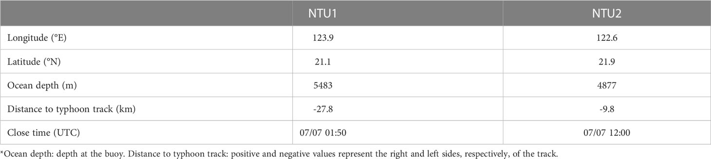
Table 1 Details of Nepartak when closest to NTU1 and NTU2^*.

TABLE 2

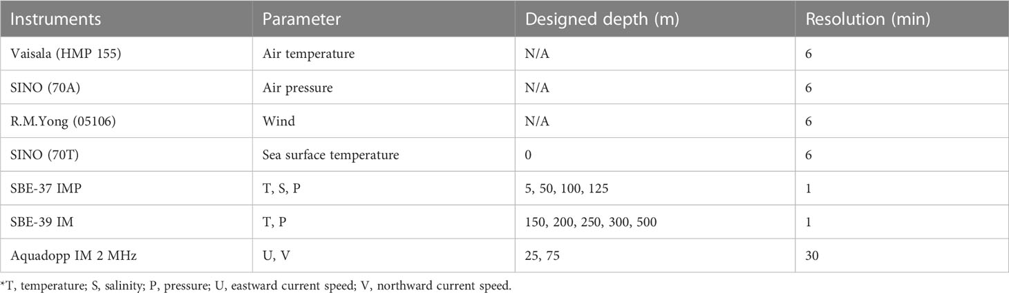
Table 2 Observation instruments and measured parameters at buoys^*.

2.4 Other data

The climatological Global Ocean Physics Reanalysis product was used to estimate the climatological mixed layer depth (MLD) and depth of the 26°C isotherm (D26) at a spatial resolution of 1/12° × 1/12°. The daily Global Ocean Physics Reanalysis product (https://resources.marine.copernicus.eu/) was used to estimate the pre-typhoon MLD and D26 (i.e., (on 4 July 2016) at a spatial resolution of 1/12° × 1/12° (i.e., approximately 8 km). The daily sea level anomalies (SLAs) and geostrophic current anomalies were taken from CMEMS (https://resources.marine.copernicus.eu/) at a spatial resolution of 0.25° × 0.25°.

2.5 Ekman pumping velocity

The wind stress from a typhoon is the main mechanism for the upper ocean response, which can cause the Ekman pumping effect. The Ekman pumping velocity (EPV, m/s) that results from Ekman pumping can be computed as follows (Price, 1981):

$\begin{array}{ll}\text{EPV}=\frac{1}{{\text{ρ}}_0}\nabla \times (\frac{\tau }{\text{f}})& (1)\end{array}$

where ${\text{ρ}}_0=1024 \text{kg}/{\text{m}}^3$ is the density of seawater, f is the Coriolis parameter, and τ is the wind stress vector (N). τ can be calculated as follows:

$\begin{array}{ll}\tau ={\text{ρ}}_{\text{a}}{\text{C}}_{\text{D}}\left|U_{10}\right|U_{10}& (2)\end{array}$

where C_D is the drag coefficient, ρ_α is the air density ($\text{kg}/{\text{m}}^3$), and U₁₀ is the 10 m wind vector (m/s). The drag coefficient can be calculated as follows (Li et al., 2021):

$\begin{array}{ll}{C}_D=\{\begin{array}{c}(4-0.6\left|U_{10}\right|)\times {10}^{-3} for \left|U_{10}\right|<5 m/s\\ (0.737+0.0525|U_{10}|)\times {10}^{-3} for 5m/s\le \left|U_{10}\right|<25m/s\\ 2.05\times {10}^{-3} for \left|U_{10}\right|\ge 25m/s\end{array}& (3)\end{array}$

2.6 Rotary spectral analysis

Rotary spectral analysis (Leaman and Sanford, 1975) is a type of spectral analysis that uses the time series of the current velocity vector, which includes clockwise (CW) and counterclockwise (CCW) spectra, to reflect the energy distribution of a characteristic rotational frequency in the CW and CCW directions, respectively. Any velocity vector can be written as $W(t)=u(t)+iv(t)$, where u, v are the east–west and north–south components, respectively, of the velocity. The Fourier transform corresponding to each wave number in the vertical direction can be expressed as $u=a_{1}cos\text{ω}t+b_{1}sin\text{ωt}$, $v=a_{2}cos\omega t+b_{2}sin\omega t$.This equation can be divided into two parts comprising the positive and negative wave numbers:

$\begin{array}{ll}u+iv=W_{+}{e}^{i\text{θt}}+W_{-}{e}^{-i\text{θt}}& (4)\end{array}$

$\begin{array}{ll}{W}_{+}=\frac{1}{2}[(a_1+b_2)+i(a_2-b1)], W_{-}=\frac{1}{2}[(a_1-b_2)+i(a_2+b_1)]& (5)\end{array}$

where $a_1,b_1,a_2,b_2$ are the component velocity amplitudes, t is the time, i is the imaginary unit, ω is the rotation angular velocity, and θ is the phase. $W_{+}, W_{-}$ are the CCW and CW rotational components, respectively, of the velocity. Their corresponding CCW and CW rotation spectra are given by

$\begin{array}{ll}{S}_{+}=\langle W_{+}{W}_{+}^{*}\rangle /2,S_{-}=\langle W_{-}{W}_{-}^{*}\rangle /2& (6)\end{array}$

where the angled brackets represent the total average and the asterisk represents the conjugate. The direction of energy propagation is the same as the direction of group velocity while the direction of group velocity propagation is opposite to the direction of the wave number. Therefore, when the direction of the wave number is upward, S_- represents the tendency of energy to propagate downward; when the direction of the wave number is downward, S₊ represents the tendency of energy to propagate upward (Leaman and Sanford, 1975).

3 Evolution of Nepartak

Nepartak was first observed as a tropical depression near 10°N, 145°E in the early morning of 3 July 2016, and it moved northwestward with steadily increasing intensity. It developed into a category 1 typhoon at 18:00 UTC on 4 July, and it was upgraded to a category 4 super typhoon at 12:00 UTC on 5 July. Its intensity continued to strengthen into a category 5 super typhoon at 00:00 UTC on 6 July with a maximum sustained wind speed of ~80 m/s (155 kn) (Figure 1, Figure 2E). The maximum wind speed decreased by ~10 m/s as Nepartak weakened from category 5 to category 4 and made its first landfall near Taitung City in southeastern Taiwan at 21:50 UTC on 7 July with a near-center wind speed of up to 55 m/s and a minimum central pressure of 920 hPa (Figures 2D, E). It made its second landfall over Shishi, Fujian Province at 05:45 UTC on 9 July with a near-center wind speed of up to 25 m/s and a minimum central pressure of 990 hPa (Figure 1). It decayed quickly after making its second landfall.

FIGURE 1

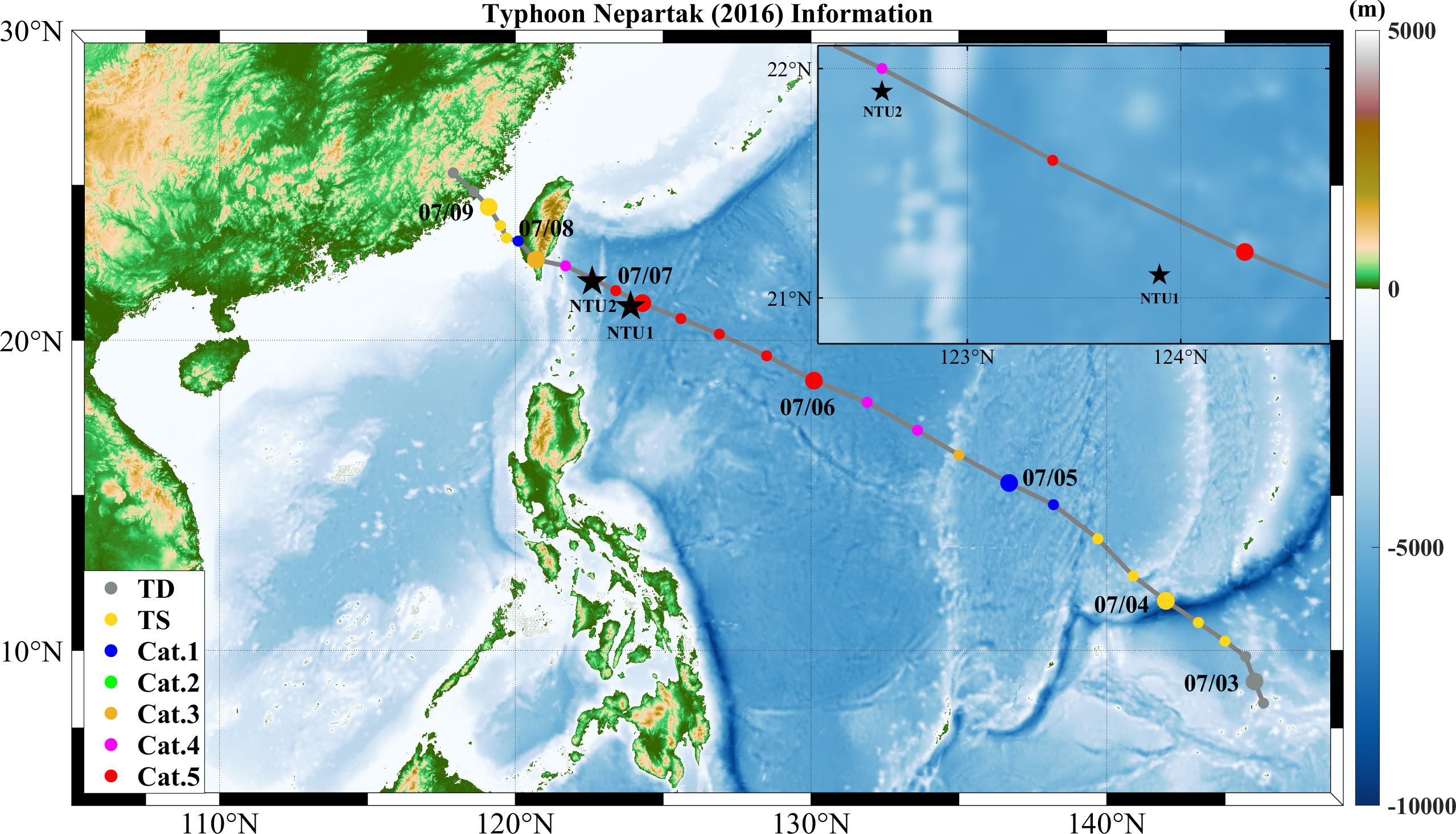
Figure 1 Tracks of Typhoons Nepartak (2016) obtained from the IBTrACS, showing their positions every 6 h (dots). The time at 0000 UTC from 3 to 9 July is labeled. The black pentagram indicates the positions of the buoy stations (NTU1 and NTU2). In the legend, TD, TS, Cat.1, Cat.2, Cat.3, Cat.4, and Cat.5 are abbreviations for tropical depression, tropical storm, category 1 typhoon, category 2 typhoon, category 3 typhoon, category 4 typhoon and category 5 typhoon, respectively. The background shade indicates the topography.

FIGURE 2

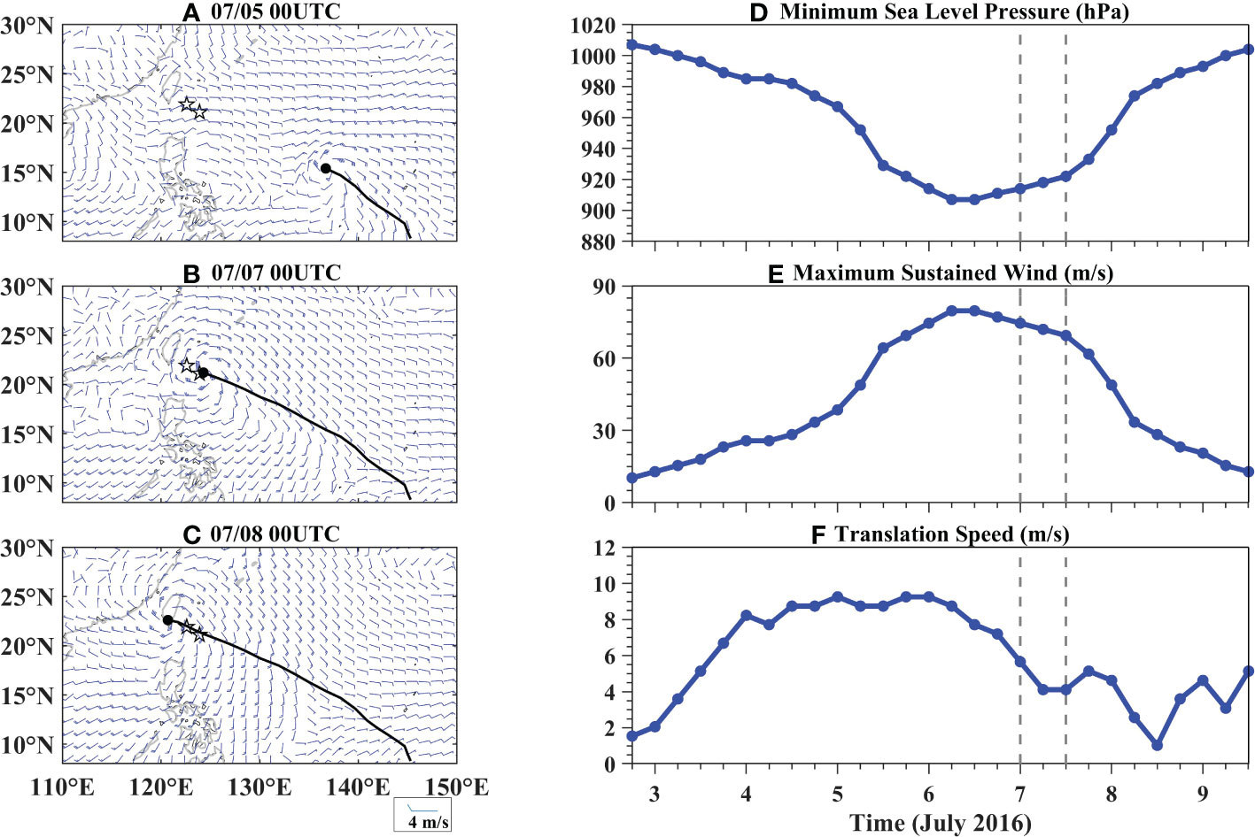
Figure 2 CCMP windbar at (A) 5 July 2016 00:00 UTC (B) 7 July 2016 00:00 UTC (C) 8 July 2016 00:00 UTC. The black curves show Nepartak’s track and the black circles indicate its center at 0000 UTC on the specified day. Also shown are temporal variations in (D) sea-level central air pressure, (E) maximum sustained wind and (F) translation speed for Typhoon Nepartak (2016).

During the buoy observation period, Nepartak was 27.8 km away from NTU1 at 01:50 UTC on 7 July, which was located to the left of the typhoon track (Figure 1). About 10 h later, the eye of the typhoon approached NTU2 at 12:00 UTC on 7 July, which was 9.8 km to the left of the typhoon track (Figure 1). Supplementary Figure 1 shows the Himawari-8 satellite image at 02:00 UTC and 12:00 UTC on 7 July. When Nepartak reached NTU1 with a well-formed and distinguishable eye, the sea level pressure at its eye decreased to 914 mbar (Supplementary Figure 1A) in the early morning of 7 July, and NTU1 observed an atmospheric pressure of 940 hPa and maximum wind gust of 41 m/s. When the eye of the typhoon reached NTU2 in the evening of 7 July, the sea level pressure at its eye was 922 mbar (Supplementary Figure 1B), and NTU2 recorded a very low pressure of 911 hPa and a maximum gust of 44 m/s.

From 18:00 UTC on 2 July to 00:00 UTC on 4 July, Nepartak continued accelerating, and it reached a moving speed of ~9.5 m/s by 00:00 UTC on 6 July (Figure 2F), after which it started to slow down. Nepartak passed the two buoys at an average speed of ~4.6 m/s as a relatively slow-moving typhoon. The non-dimensional moving speed is the ratio of the local inertial period to the typhoon residence time and can be calculated as S = πU_h/(4R_maxf), where U_h is the typhoon translation speed, f is the local inertial frequency, and R_max is the maximum wind radius (Price et al., 1994). When the non-dimensional moving speed is close to 1, the typhoon residence time is comparable to the local inertial period, and the response of the upper ocean should contain strong inertial motions (Wang et al., 2012). Nepartak had a non-dimensional moving speed of S = 2.32 at the buoys, which suggests a relatively strong inertial motion.

Supplementary Figure 2 displays the distribution of the daily accumulated precipitation during the passage of Nepartak. The rainfall was mainly distributed near the eye wall of the typhoon, but some heavy precipitation was also outside it. As Nepartak gradually intensified, spiral rain bands were established. Precipitation at NTU1 and NTU2 was mainly concentrated on 6–8 July. The asymmetry in rainfall distribution can be attributed to the southwest monsoon and topography with increased convective precipitation to the left of the typhoon track (Corbosiero and Molinari, 2003; Xu et al., 2014).

4 Results

4.1 Pre-typhoon ocean conditions

The atmospheric and oceanic factors along a typhoon’s path influence how it develops over the ocean. Before the passage of Nepartak, easterly winds with a maximum wind speed of ~6 m/s prevailed in the Philippine Sea on 4 July 2016. The southwest monsoon transported a warm and humid airflow promoting convection and cloud system development, which was conducive to the development of Nepartak (Figure 2A). The temperature of the upper ocean is also thought to play a significant role in the development of typhoons. The SST was greater than 29°C along the typhoon track with a peak of nearly 31°C (Figure 3A). D26 defines the depth of the warm water layer according to the threshold temperature of 26°C, and it is used to measure the upper ocean heat content (Hsieh et al., 2017). Figures 3B, D show the climatological D26 and D26 on 4July. Before the passage of the typhoon, D26 was thicker than 90 m along most of the typhoon track. Although D26 was shallower at the two buoys, it was still about 80 m thick.

FIGURE 3

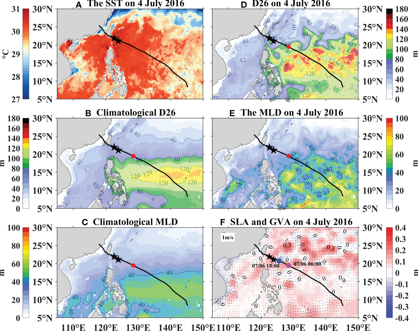
Figure 3 Pre-storm distributions of (A) SST on 4 July 2016, (B, D) depths of the 26°C isotherm, (C, E) mixed layer depth, (F) sea level anomaly and geostrophic currents anomaly on 4 July 2016. (B, C) are estimated based on climatological global ocean reanalysis product, (D, E) on the global ocean reanalysis for 4 July 2016. The black curve denotes the best track of Nepartak. The black pentagrams indicate the buoy stations. The red dots in (C–F) and the pink dot in (B) indicate the position where Nepartak reached its peak. The blue dots indicate the position where Nepartak started to weaken. SST, sea surface temperature, D26, the depths of the 26°C isotherm, MLD, the mixed layer depth, SLA, sea level anomaly, GVA, geostrophic currents anomaly.

The MLD is the depth at which the water temperature is 0.5°C lower than the SST (Nishikawa and Yasuda, 2011). Figures 3C, E show the distribution of the climatological MLD and MLD on 4 July. The background MLD affects the typhoon intensity (Zhao and Chan, 2017). For a given translation speed, a higher SST and a greater D26 or MLD means that the SST will not decrease sharply after passage of a typhoon churns stirs up the upper ocean, which is more conducive for typhoon intensification (Hsieh et al., 2017). Both the results estimated from the daily Global Ocean Physics Reanalysis product and derived from the climatological Global Ocean Physics Reanalysis product displayed a common feature: in most marine areas south of 20° N in the Northwest Pacific, D26 was thicker than 80 m, and MLD was deeper than 40 m. In particular, the pre-typhoon D26 on 4 July was thicker than the climatological D26 at about 120 m along the track of Nepartak south of 20°N. The integrated ocean conditions (i.e., SST > 29°C, MLD > 40 m, D26 > 120 m) favored the intensification of Nepartak (Zhao and Chan, 2017), which may explain why it continued to strengthen after its generation and reached its peak (red dots in Figure 3) at 06:00 UTC on 6 July. Another important factor in the development of a typhoon is whether it passes over a warm water surface or eddy to gain energy through heat flux exchange or passes over a cold water surface or eddies to lose energy (Jangir et al., 2021). Figure 3F shows the distribution of SLAs and geostrophic current anomalies on 4 July. Before Nepartak reached its peak intensity (pink dot), most of the area it passed through had weak warm mesoscale eddies. When Nepartak passed through areas with significant SLAs at 06:00 UTC on 6 July, there was a weak warm anticyclone on the left side of the typhoon track (127°E, 19.5°N), and the SLA value was 0.2 m higher at the center than at the edge area. Meanwhile a relatively strong warm anticyclone was on the right side of the typhoon track (131°E, 20.3°N) for which the SLA value was 0.3 m higher at the center than at the edge area. Hence, Nepartak peaked as it passed over an area with warm eddies, a thick warm water layer, and a deep MLD, which supplied it with energy. After 12 h (18:00 UTC on 6 July), Nepartak passed over a cold mesoscale eddy for which the SLA value was 0.15 m lower at the center than at the edge area, where D26 was less than 40 m (Figure 3D) and MLD was less than 20 m (Figure 3E). The high SST combined with a thinner D26 and shallower MLD meant that the SST decreased as the typhoon passed through and churned up the upper ocean, which suppressed subsequent intensification. This is when Nepartak began to weaken (blue dot in Figure 3F). Although Nepartak later passed over a relatively strong warm eddy, the shallow D26 meant that the typhoon-induced vertical mixing/entrainment easily penetrated the mixed layer, which brought cold water of the thermocline layer into the upper layer and weakened Nepartak.

4.2 Evolution of air–sea parameters

The temporal evolution of atmosphere parameters (i.e., wind, air temperature, air pressure), the SST, and the air–sea heat flux at NTU1 and NTU2 were analyzed before, during, and after the passage of Nepartak. The air–sea heat flux includes the following components: the shortwave radiation (Q_sw), longwave radiation (Q_lw), sensible heat flux (Q_sen), and latent heat flux (Q_lat). All of these have been calculated using the bulk parameterization by the research in Yang et al. (Fairall et al., 2003; Yang et al., 2019).

Figure 4 shows that, before the passage of Nepartak, the background wind at the two buoys was dominated by easterly winds with a wind speed of less than 10 m/s. This is consistent with the CCMP wind data (Figure 2A). The sea level pressure was about 1010 hPa at both buoys. The SSTs were 30.5°C and 30.8°C at NTU1 and NTU2, respectively, while the air temperature fluctuated around 30°C at both buoys. Before Nepartak, Q_lat and Q_sen were about −200 and 4 W/m², respectively, at NTU1 and −140 and 3 W/m², respectively, at NTU2. The variation in the radiant heat flux (Q_sw + Q_lw) was small with an obvious diurnal variation. The net heat flux (Q_net = Q_sw + Q_lw + Q_sen + Q_lat) was mainly dominated by the radiant heat flux, which indicates that the ocean mainly gained heat from solar radiation. The time evolution figure of heat flux (Figures 4G, H) is similar to Yang et al. (Yang et al., 2019).

FIGURE 4

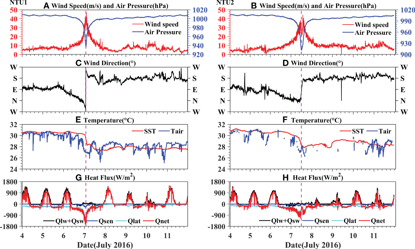
Figure 4 Buoy observed air-sea variables at NTU1 and NTU2 during 4–11 July 2016. (A, B) air pressure (blue line) and wind speed (red line). (C, D) wind direction. Regarding the wind directions, N, W, S, and E indicate the approach directions of the winds, namely, north, west, south, and east, respectively. (E, F) surface air temperature (blue line) and sea surface temperature (red line). (G, H) Buoy data-derived net air-sea heat flux (Qnet, red line), net radiation heat flux (Qsw+Qlw, black line), latent heat flux (Qlat, cyan line), and sensible heat flux (Qsen, blue line). The magenta vertical dashed lines indicate the time at a minimum air pressure.

When Nepartak was approaching the buoys, the wind speed gradually increased (Figure 2B), and the air pressure gradually decreased. NTU1 recorded an air pressure of 940 hPa, maximum wind gust of 41 m/s, and decrease in SST from 30.5°C to 28.3°C when the eye of Nepartak approached. After a few hours, the eye of Nepartak approached NTU2, which recorded a relatively low air pressure of 911 hPa, maximum wind gust of 44 m/s, and drop in the SST from 30.8°C to 28.1°C. The wind direction was counterclockwise when Nepartak passed the two buoys, which means that they were on the left side of the typhoon track. This is consistent with Figure 1. The air pressure was 29 mbar lower at NTU2 than at NTU1 because the former was closer to the eye of the typhoon. NTU2 showed double peaks in the wind speed with an intervening minimum (Figure 4B) accompanied by a sharp change in wind direction (north to south), which means that it passed through the eye (Supplementary 1B). During the passage of Nepartak, the air temperature dropped by about 4.5°C at NTU1. There were significant gaps in the air temperature data at NTU2, but the remaining data indicated a significant decline. The solar radiation was almost zero due to cloud cover (Supplementary 1). Qnet reached about −1600 and −1440 W/m² at NTU1 and NTU2, respectively, which indicates that the air–sea interface heat exchange was very strong and that the atmosphere absorbed a significant amount of heat from the ocean. Qlat decreased significantly and reached about −1140 and −950 W/m² at NTU1 and NTU2, respectively. These account for 90% and 83%, respectively, of Qnet, which suggests that the heat transfer from the ocean to the atmosphere was the main contributor to the latent heat flux. Therefore, during the passage of a typhoon, the drastic change in air–sea parameters is an important mechanism for how the typhoon affects the ocean. After the passage of Nepartak, the background wind at the two buoys was dominated by southerly winds with a wind speed of about 10 m/s (Figure 2C), and the sea level pressure gradually rose to 1005–1010 hPa. One day after the typhoon, the SSTs at the two buoys fell to minimum values of 27.3°C and 27.8°C, respectively.

4.3 Surface response

Figure 5 shows the SST evolution during the passage of Nepartak from 4 to 8 July according to satellite data. Before Nepartak passed through, the Northwest Pacific was 29°C–31°C (Figure 5A); this is much warmer than the threshold value of 26°C, which is typically considered the minimum SST at which a storm can develop. The SST cooling was slightly biased to the right side of the typhoon track and gradually recovered after the cold wake. The magnitude of the SST cooling was small at about 1°C–2°C (Figures 5B, C) because of the pre-typhoon conditions, such as a thicker warm water layer and deeper mixed layer. When Nepartak passed the buoys on 7 July, the SST dropped to ~28°C on the right side of the eye, and increased cooling was observed near the typhoon track (Figure 5D). The SST cooling became more pronounced as the warm water layer became thinner (Figure 3D) and the mixed layer became shallower (Figure 3F). One day after the passage of Nepartak, the SST dropped to ~27°C on the right side of the typhoon track near the buoys with an obvious large patch of cold water. Figure 5F displays the SST cooling caused by Nepartak, which was calculated as the difference between the SSTs on 4 and 8 July. A maximum SST cooling of about 4°C was observed on the right side of the typhoon track near NTU1, which may have been caused by the combination of increased latent and sensible heat losses at the surface, more vigorous vertical mixing because of enhanced vertical velocity shear, and the injection of more kinetic energy through surface wave breaking (Yang et al., 2019; Wu et al., 2020).

FIGURE 5

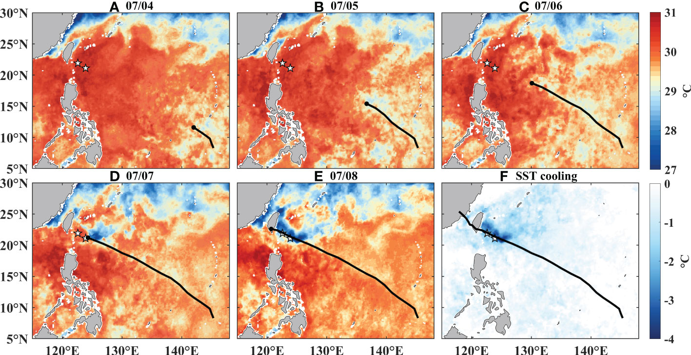
Figure 5 Daily satellite microwave optimally interpolated sea surface temperature on 4 and 8 July 2016 (A–E) and their difference (F), the latter minus the former). The black lines indicate the best track of Nepartak track and black dots indicate the centers of the tropical cyclones at 0000 UTC on that day. The white pentagrams indicate the buoy stations.

Similar to the SST response, the SSS also had anomalies on the left and right sides of the typhoon track. Figure 6 shows an 8-day running mean of the SSS map from the SMAP satellite before, during, and after Nepartak. The change in SSS induced by the typhoon was calculated as the difference between the SSS values on 4 and 8 July. The salinity primarily increased on the right side of the typhoon track and decreased on the left side. The increase in salinity on the right side can be attributed to the CW rotation of the wind stress vector on this side and resonant coupling with the mixed layer current (Price, 1981). The positive salinity anomalies on the right side of the typhoon track were less than 0.5 psu before the typhoon passed over the buoys because of the thick warm water layer in the upper ocean, which made it more difficult to bring the saltier water of the thermocline to the surface. As Nepartak passed over the buoys, the strong turbulent mixing easily penetrated the thinner mixed layer, which brought the saltier water from the thermocline to the mixed layer and increased the SSS. A positive salinity anomaly of about 0.6 psu was observed on the right side of the typhoon track near NTU1. Negative salinity anomalies were observed on the left side of the typhoon track, which can be attributed to the heavier precipitation on this side (Supplementary Figure 2). Among the five main factors for changes in salinity (i.e., vertical mixing, entrapment, advection, precipitation, and evaporation) (Delcroix et al., 1996; Perigaud et al., 2003; Liu et al., 2007), only precipitation decreases the SSS. In addition, advection of fresh water from another region may also decrease the local SSS (Hu and Zhao, 2022). Previous studies have shown that precipitation is greater on the left side of a typhoon than on the right side because of vertical wind shear, tropical cyclone motion, water vapor flux, and topography (Burpee and Black, 1989; Corbosiero and Molinari, 2003; Ueno, 2007; Chen et al., 2010; Xu et al., 2014; Gao et al., 2018). There was clearly more precipitation on the left side of Nepartak’s track, especially, the maximum precipitation is mainly concentrated on the left, which resulted in a significant negative salinity anomaly on this side (Figure 6F).

FIGURE 6

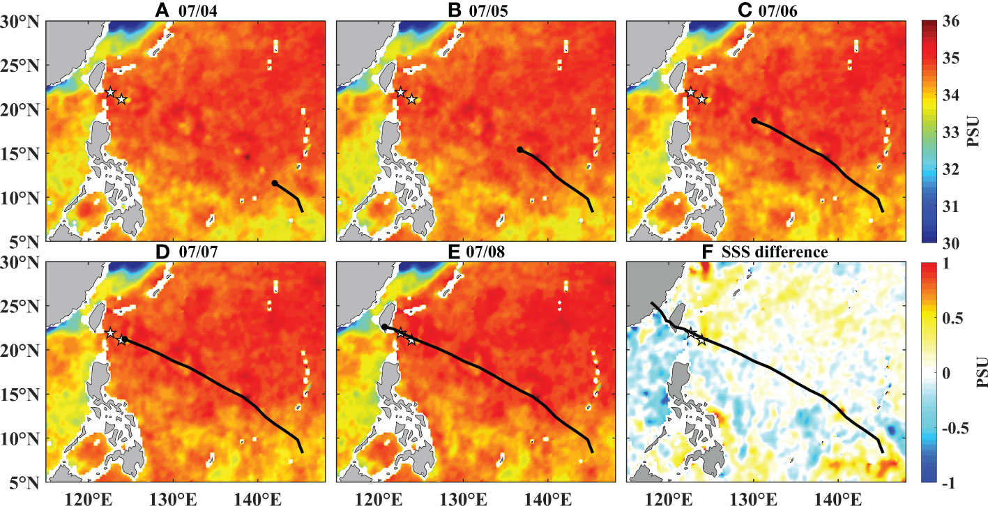
Figure 6 Daily 8 day running mean Soil Moisture Active Passive (SMAP) satellite sea surface salinity on 4 and 8 July 2016 (A–E) and their difference (F), the latter minus the former). The black lines indicate the best track of Nepartak and black dots indicate the centers of the tropical cyclones at 0000 UTC on that day. The white pentagrams indicate the buoy stations.

4.4 Subsurface response

Typhoons can cause not only a surface response of an ocean but also a subsurface response. Figure 7 shows the temporal evolution of the subsurface temperature response of the upper ocean at depths of 2–150 m as observed by NTU1 and NTU2. Temperature profile anomalies, which were defined as the time series of the temperature profile minus the average pre-typhoon value (4 July), are also shown to highlight the effect of the typhoon on the thermal structure of the ocean subsurface. The evolution of MLD (black line for NTU1, green line for NTU2) with time is also superimposed on the figure.

FIGURE 7

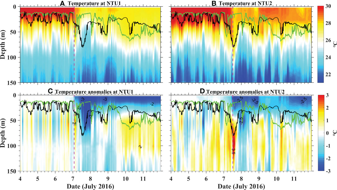
Figure 7 Temperature and Temperature anomalies during Nepartak for Buoy NTU1 (left column) and Buoy NTU2 (right column). Here, the temperature anomalies are defined as the time series of temperature profile minus the averaged value of pre-storm (4 July). The panels show (A, B) temperature, and (C, D) temperature anomalies. The magenta vertical dashed lines indicate the time when Nepartak was nearest to Buoy. The green and black curves indicate variations in mixed layer depth at NTU1 and NTU2, respectively.

Before Nepartak, the MLD fluctuated moderately around 13 m at NTU1 and fluctuated dramatically at 10–40 m at NTU2. This may be because of the combined effects of diurnal variation in solar radiation and tidal dynamics because NTU2 was closer to the shore and more susceptible to tidal influence than NTU1 (Wu et al., 2020). NTU1 started responding to Nepartak in the early morning of 7 July, and NTU2 responded several hours later. The water cooled significantly in the upper 40 m with a maximum cooling of about −3°C at NTU1 and −2.5°C at NTU2. The two buoys showed a significant difference in the MLD response. According to NTU1, the MLD increased rapidly to about 55 m a few hours before Nepartak passed and then decreased, and it increased again to about 60 m when Nepartak had passed. In contrast, NTU2 showed that the MLD gradually increased a few hours before Nepartak passed and reached a maximum of about 80 m when it passed. This may explain why NTU1 observed greater cooling than NTU2 did. After Nepartak, the MLD floated up and down due to the near-inertial oscillation of the current. At the depth of 50–120 m, the water at NTU1 initially cooled and then warmed (Figure 7C), and the water at NTU2 alternately warmed and cooled (Figure 7D). Thus, the subsurface layer had alternating warm and cold anomalies, which was especially obvious at NTU2. The maximum warm anomalies in the subsurface layer at NTU1 and NTU2 were about 2 and 3.5, respectively. In the direct forced stage (7 July), there was a strong warm anomaly in the subsurface layer at NTU2 where mixed warming was dominant; meanwhile, the subsurface layer was dominated by cold anomalies at NTU1, where the cooling effect of upwelling was significantly stronger than the warming effect caused by mixing. This also explains why the magnitude of cooling in the upper 40 m depth was greater at NTU1 than at NTU2.

To demonstrate the net effect of Nepartak on the subsurface thermal structure at the two buoys, the temperature time series of 7–9 July were averaged, including the direct forced period and early relaxed period, to obtain mean temperature anomalies. Figure 8 shows that the entire upper ocean was cooled at NTU1 during the direct forced period and early relaxed period. At NTU2, there was a cold anomaly in the uppermost 60 m, warm anomaly at 60–150 m, and negative anomaly below 150 m. Overall, NTU1 recorded cooling of the whole upper ocean, and NTU2 recorded a clear three-layer structure for the vertical response comprising a cooler surface and deep layer with a warmer layer in between.

FIGURE 8

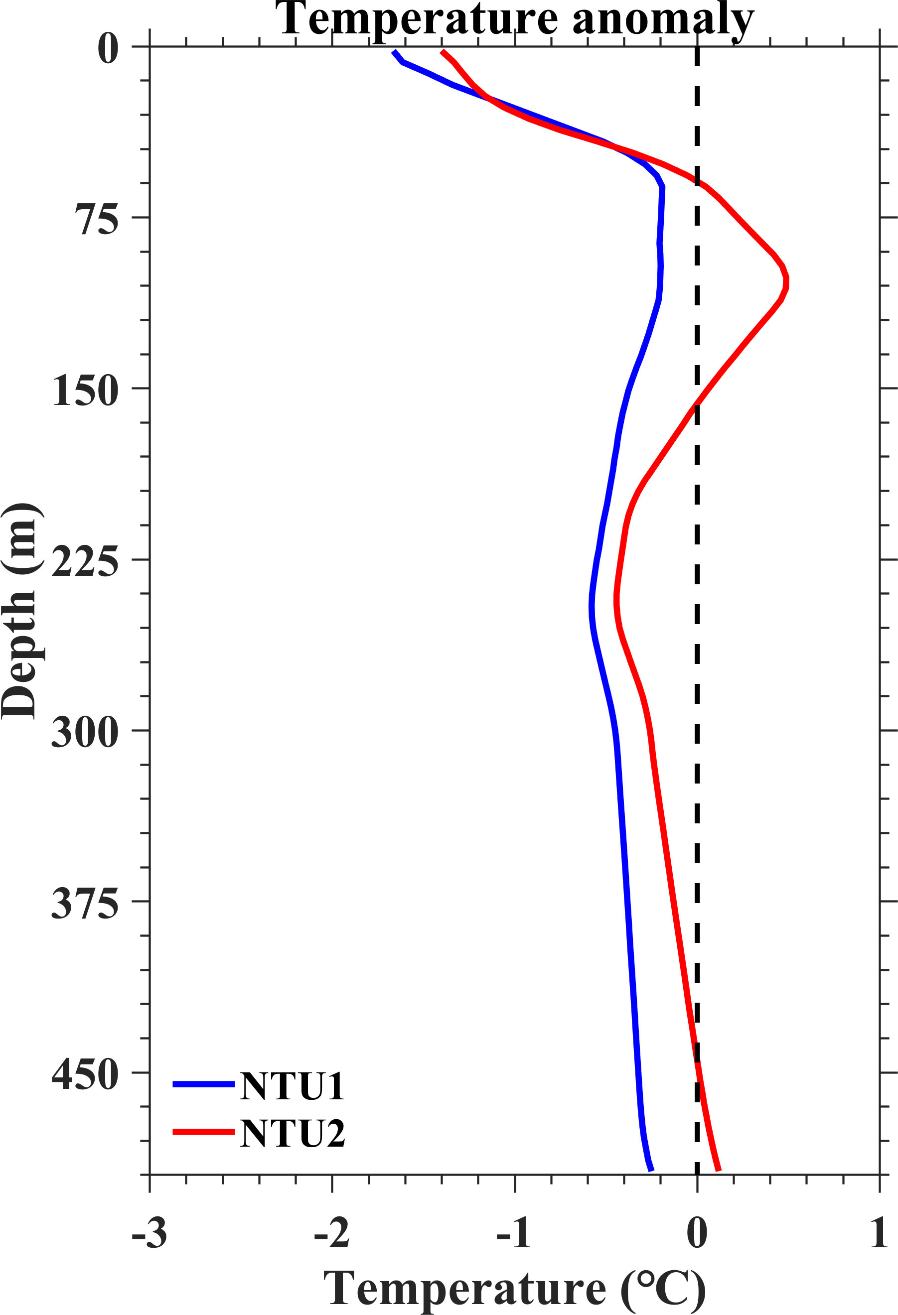
Figure 8 Mean temperature anomalies averaged over the period of 0000 UTC 7 July to 2355 UTC 9 July for NTU1(bule line) and NTU2 (red line).

The passage of a typhoon inputs a large amount of mechanical energy to the ocean (Sriver and Huber, 2007; Liu et al., 2008). In addition to enhanced local mixing, this energy is also transmitted into the ocean interior in the form of near-inertial oscillations (Gill, 1984). In this study, the ocean currents observed by NTU1 and NTU2 at a depth of 75 m were analyzed.

Figure 9 shows the eastward current component (U-component), northward current component (V-component), and current vector of the two buoys at a depth of 75 m. For the U-component, NTU1 observed a notable increase in the current speed during Nepartak from about 10 to 60 cm/s while NTU2 observed an increase from about 10 to 21 cm/s. This is mainly due to the fact that NTU2 was closer to the typhoon eye than NTU1 (Supplementary Figure 1) and the intensity of typhoon at NTU1 was stronger than at NTU2. Therefore, the energy input into the ocean interior at NTU2 is smaller than at NTU1, the near-inertial current at NTU2 was smaller than at NTU1. The current velocity exhibited significant oscillations (Figures 9A, B). The increase in current velocity was accompanied by a significant increase in the current period. As the kinetic energy dissipated, the current velocity and period also gradually decreased. On 14 July, the inertial oscillation attenuated to the state before the typhoon, which indicates that it persisted for 7 days. This agrees with previous studies showing that storm-induced near-inertial oscillations typically last 7 days or more (Qi et al., 1995; Teague et al., 2007).

FIGURE 9

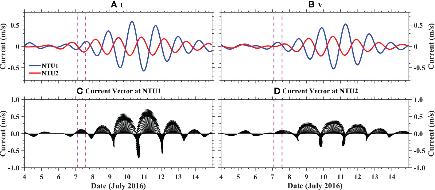
Figure 9 Buoy observed variables at NTU1 and NTU2 during 4–14 July 2016. (A) eastward current component, (B) northward current component, and (C, D) current vector at 75 m depth. The magenta vertical dashed lines indicate the time when Nepartak was nearest to Buoy.

To further study the characteristics of the near-inertial oscillations induced by the typhoon, the CW and CCW rotation power spectra were obtained at a depth of 75 m. Figure 10 shows that the extreme value point of the near-inertial oscillation energy corresponded to a frequency close to the local inertial frequency. The energy was mainly concentrated at the local inertial frequency (f1 and f2) and diurnal internal tide frequency (O₁, K₁), and the energy spectral magnitude of the semidiurnal internal tide (M₂, S₂) was less than 10⁰ m²/s²/cpd (cpd: cycle per day). Near the inertial frequency, both the CW and CCW rotation spectra had maximum values. The CW energy spectrum had greater values than the CCW energy spectrum, which indicates that the down-transmission and up-transmission characteristics of the near-inertial oscillation coexisted but the CW energy was dominant, as demonstrated by the stronger down-transmission characteristics. The energy spread to the deep ocean from the ocean surface; in other words, the energy transmitted into the ocean was mainly from Nepartak.

FIGURE 10

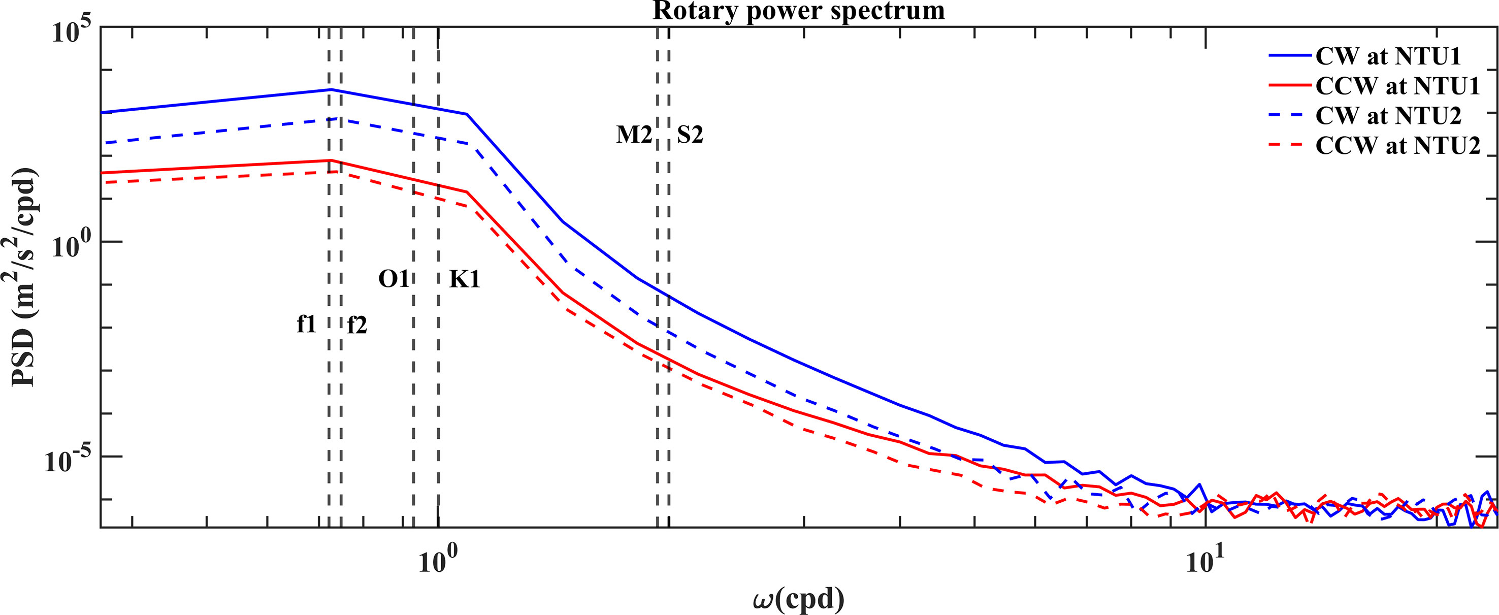
Figure 10 The diagram of energy rotation power spectrum at buoy NTU1 and NTU2, respectively. The blue solid lines represent the clockwise (CW) rotation power spectra at NTU1, the red solid lines represent the counterclockwise (CCW) rotation power spectra at NTU1, the blue dashed lines represent the clockwise (CW) rotation power spectra at NTU2, the red dashed lines represent the counterclockwise (CCW) rotation power spectra at NTU2. The black dashed lines represent local inertial frequency (f1 and f2), diurnal tide frequency (K₁ and O₁), semidiurnal tide frequency (M₂ and S₂).

4.5 Differences in the ocean response at the two buoys

Two buoys located 350 and 150 km off the coast of Taiwan accurately captured the characteristics of the upper ocean response caused by Nepartak. Both buoys were on the left side of the typhoon track and suffered similar typhoon factors (e.g., typhoon intensity and translation speed) during its passage. However, the subsurface temperature responses differed significantly during the direct forced period (7 July) and early relaxed period (8-9 July) at the two buoys. At NTU1, the entire upper ocean experienced strong cooling; at NTU2, the subsurface experienced warming. Typhoons are known to significantly affect the thermal structure of the upper ocean, where the dominant mechanisms are heat pumping and cold suction. Strong wind stirring enhances vertical mixing in the upper ocean, which causes warm water to roll down and cold water to surge up. After the passage of a typhoon, the SST gradually recovers due to solar radiation at the air–sea interface while the warm anomalies in the subsurface layer remain; this generates a net heat input, which is the heat pump effect (Emanuel, 2001). Meanwhile, the cyclonic wind stress of typhoons can cause strong upwelling that cools the entire upper ocean, which is known as cold suction (Price, 1981; Zhang et al., 2016). For actual typhoons, the heat pump and cold suction mechanisms jointly affect the thermal response of the upper ocean, which results in a decrease in the SST and a complex variability in the subsurface temperature (Zhang, 2022).

As Nepartak passed over the buoys, significant SST cooling along the typhoon track was observed due to the deepening of the mixed layer, release of heat from the ocean to the atmosphere through the latent heat flux (Figures 4G, H), and upwelling near the eye. The temporal evolution of the temperature profiles at the two buoys (Supplementary Figure 3) indicated that, when Nepartak passed NTU1 (7 July), the oceanic thermocline was strongly uplifted because of the cyclonic wind stress, which cooled the entire upper ocean. This indicates that cold suction was the main mechanism. when Nepartak passed through NTU2, not only the surface layer was cooled but also the subsurface layer was warmed, the vertical mixing seemed to be the dominant mechanism. Thus, the importance of mixing (heat pumping) or upwelling (cold suction) differed according to where the typhoon passed through the buoys. Figure 11 exhibits the temporal evolution of the wind stress and Ekman pumping velocity at the two buoys. When Nepartak passed NTU1 (7 July), the wind stress was slightly stronger than that at NTU2 while the Ekman pumping velocity was weaker than that at NTU2. However, the upper ocean presented a three-layer structure at NTU2 while was cooled at NTU1 on 7 July (Figure 8), which indicates that other factors affected the change in the upper ocean temperature at NTU1. Figure 12 displays the evolution of SLAs during Nepartak. There was a cold eddy at NTU1 when Nepartak passed by on 7 July while NTU2 had zero SLAs. The cold eddy induced by the typhoon may have contributed to the cooling of the entire upper ocean at NTU1. Figure 13 shows a simplified sketch of the vertical temperature profiles when typhoon Nepartak passed the two buoys. The upper ocean temperature response shows a two-layer vertical structure consisting of cooler surface and warmer subsurface layer in the case of only mixing (Figure 13A). When Nepartak passed NTU1, strong upwelling cause by cold eddy cooled the entire upper ocean (Figure 13C), while the vertical mixing caused by wind stress was stronger than the upwelling caused by wind stress curl at NTU2 (Figure 13B). Thus, during the direct forced period (7 July), the cold eddy and upwelling may have been the main mechanism for the subsurface temperature anomalies at NTU1, while vertical mixing was dominant at NTU2.

FIGURE 11

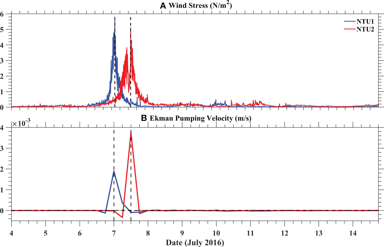
Figure 11 The temporal evolution of wind stress (A) and Ekman pumping velocity (B) at buoy NTU1 and NTU2, respectively. The gray vertical dashed lines indicate the time when Nepartak was nearest to Buoy.

FIGURE 12

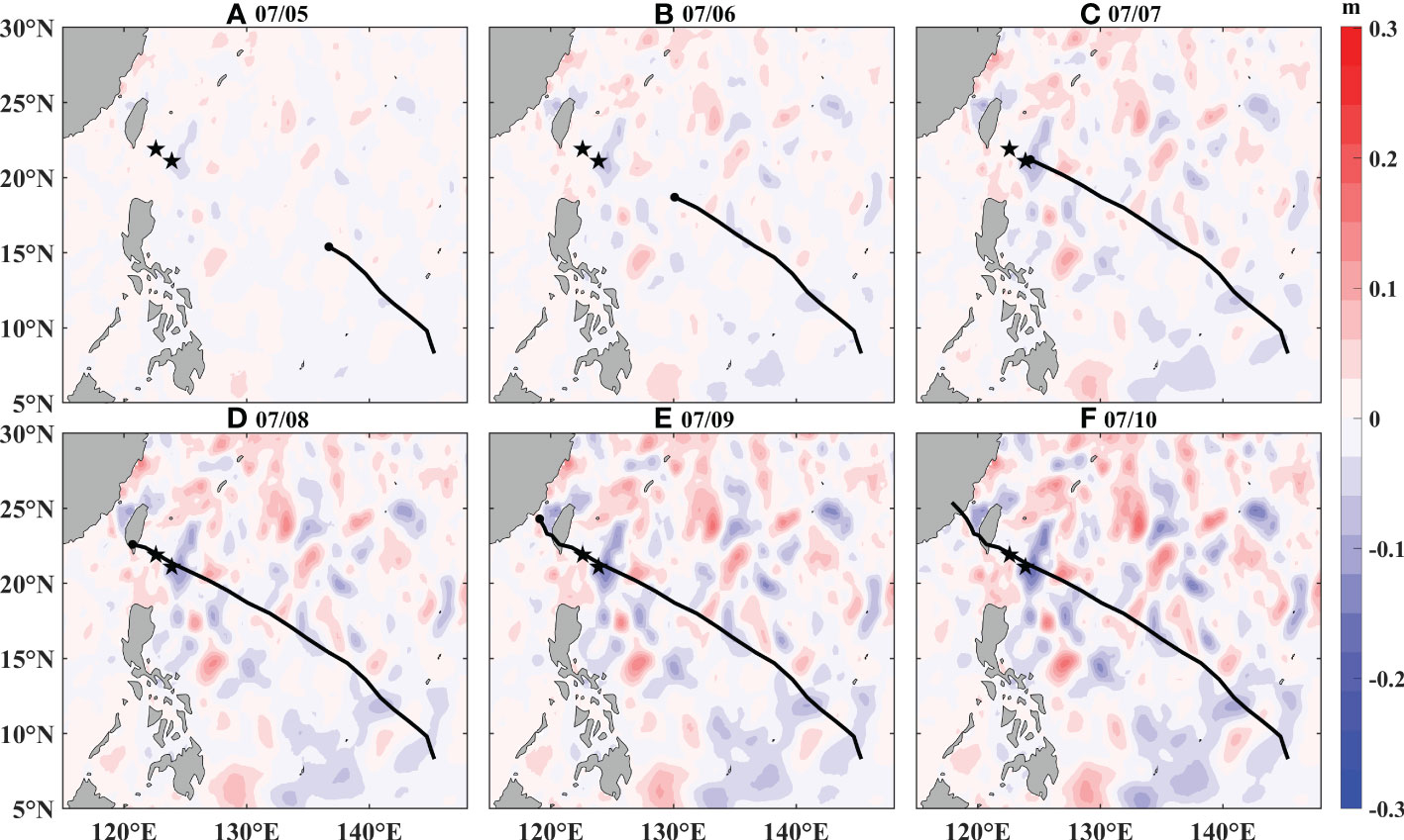
Figure 12 Daily SLA distribution during typhoon Nepartak. (A, B) before the passage of Nepartak; (C, D) during the passage of Nepartak; (E, F) after the passage of Nepartak. The black lines indicate the best track of Nepartak and black dots indicate the centers of the tropical cyclones at 0000 UTC on that day. The black pentagrams indicate the buoy stations.

FIGURE 13

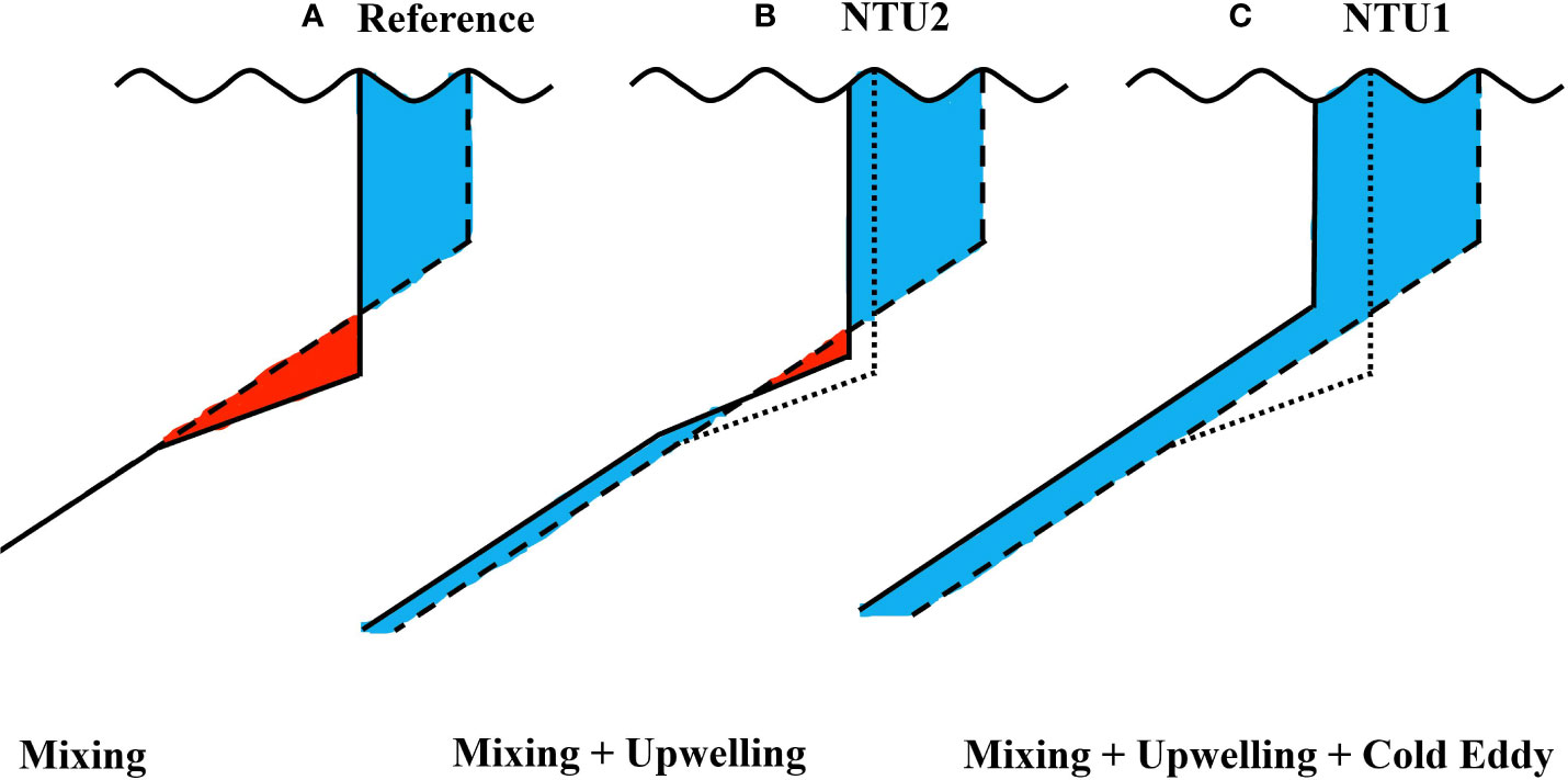
Figure 13 Sketch of the vertical temperature profiles during typhoon “Nepartak” that caused by before (dashed lines) and after (solid lines) (A) only mixing (as a reference), (B) composition of mixing and upwelling, and (C) composition of mixing, upwelling and cold eddy. The dotted lines in (B, C) indicate the temperature profiles caused by only mixing. The red and the blue shadings indicate the warming and cooling anomaly, respectively.

5 Discussion and conclusions

Although many prior observational studies have focused on the upper ocean response to typhoons, there is still a lack of comprehensive understanding of the underlying processes during super typhoons, especially near the eye. In July 2016, two buoys deployed off the coast of southeastern Taiwan captured data on the upper ocean response to the category 5 Super Typhoon Nepartak within 30 km of the eye, which provided a rare opportunity to better understand typhoon–ocean interactions and improve predictions of typhoon intensity for disaster mitigation. Observational data from the two buoys and satellite remote sensing data were used for a systematic analysis on the atmospheric and oceanic parameters during the passage of Nepartak. Some new findings were obtained to supplement typical response characteristics that are already known, such as cooling of the SST on the right side of the typhoon path:

1) The high SST (>29°C), thick warm water layer (D26 > 120 m) and deep mixed layer (MLD >40 m) provided a good thermal environment for continuous intensification of the typhoon. The appearance of a cold eddy, thinner warm water layer (D26< 40 m), and shallow mixed layer (MLD< 20 m) made it easier for the cold water of the thermocline to enter the mixing layer, which made the typhoon begin to weaken.

2) During the direct forced period and early relaxed period, the upper ocean temperature response showed different structures at the two buoys on the left side of Nepartak. At NTU1, which was 27.8 km to the left of the typhoon, the entire upper ocean was cooled. At NTU2, which was 9.8 km to the left of the typhoon, there was a clear three-layer vertical structure consisting of cooler surface and deep layers with a warmer layer between.

3) The mechanism for the change in subsurface temperature in the direct forced period differed at the two buoys. The main mechanism for subsurface temperature anomalies was the cold eddy and upwelling at NTU1 and vertical mixing at NTU2.

4) The typhoon-generated near-inertial energy was mainly concentrated in the local inertial frequency and diurnal internal tide frequency and showed stronger down-transmission characteristics.

These high-quality observations of Nepartak are unique. The two buoys captured two distinct subsurface ocean responses, which was attributed to competition between two typical ocean response mechanisms. Under similar preexisting oceanic conditions, the movement of ocean eddies under typhoon forcing was an unexpected mechanism leading to the dominance of upwelling, which needs to be considered for predicting changes in the ocean environment and typhoon intensity. The two buoys were moored at 30 and 10 km to the left side of the typhoon track, but no observations were made on the right side. A more detailed discussion on the main mechanisms causing temperature anomalies on both sides of the typhoon track is beyond the scope of the present work due to the lack of high-quality in situ observations. This topic will be examined in future studies by numerical simulation to further quantify the contributions of different physical processes to subsurface temperature anomalies.

Data availability statement

The original contributions presented in the study are included in the article/Supplementary Material. Further inquiries can be directed to the corresponding authors.

Author contributions

HW performed the data analysis and wrote the initial draft. JL proposed the main ideas and dramatically modified the manuscript. JS and CZ all participated in the discussion and contributed to the improvement of the manuscript. All authors contributed to the article and approved the submitted version.

Funding

The National Natural Science Foundation of China (No.41605070), the Project supported by Innovation Group Project of Southern Marine Science and Engineering Guangdong Laboratory (Zhuhai) (No. 311022001), the Project of Southern Marine Science and Engineering Guangdong Laboratory (Zhuhai) (No. SML2021SP207).

Acknowledgments

We thank Professor Yiing-Jang Yang for providing the high-quality buoy observation data.

Conflict of interest

Author DK is employed by Xiamen Ocean Engineering Exploration and Design Institute Co. Ltd.

The authors declare that the research was conducted in the absence of any commercial or financial relationships that could be construed as a potential conflict of interest.

Publisher’s note

All claims expressed in this article are solely those of the authors and do not necessarily represent those of their affiliated organizations, or those of the publisher, the editors and the reviewers. Any product that may be evaluated in this article, or claim that may be made by its manufacturer, is not guaranteed or endorsed by the publisher.

Supplementary material

The Supplementary Material for this article can be found online at: https://www.frontiersin.org/articles/10.3389/fmars.2023.1132714/full#supplementary-material

References

Bond N. A., Cronin M. F., Sabine C., Kawai Y., Ichikawa H., Freitag P., et al. (2011). Upper ocean response to typhoon choi-wan as measured by the kuroshio extension observatory mooring. J. Geophys. Res.: Oceans 116. doi: 10.1029/2010JC006548

CrossRef Full Text | Google Scholar

Burpee R. W., Black M. L. (1989). Temporal and spatial variations of rainfall near the centers of two tropical cyclones. Monthly Weather Rev. 117, 2204–2218. doi: 10.1175/1520-0493(1989)117<2204:TASVOR>2.0.CO;2

CrossRef Full Text | Google Scholar

Chang D. H.-I., Ma Y.-F., Her M. W.-H., Yang Y.-J., Chang M.-H., Jan S., et al. (2017). The NTU buoy for typhoon observation, part 1: System. OCEANS conferences, 1–5. doi: 10.1109/OCEANSE.2017.8084822

CrossRef Full Text | Google Scholar

Chen L., Li Y., Cheng Z. (2010). An overview of research and forecasting on rainfall associated with landfalling tropical cyclones. Adv. Atmos Sci. 27, 967–976. doi: 10.1007/s00376-010-8171-y

CrossRef Full Text | Google Scholar

Chiang T.-L., Wu C.-R., Oey L.-Y. (2011). Typhoon kai-tak: An ocean’s perfect storm. J. Phys. Oceanography 41, 221–233. doi: 10.1175/2010JPO4518.1

CrossRef Full Text | Google Scholar

Corbosiero K. L., Molinari J. (2003). The relationship between storm motion, vertical wind shear, and convective asymmetries in tropical cyclones. J. Atmospheric Sci. 60, 366–376. doi: 10.1175/1520-0469(2003)060<0366:TRBSMV>2.0.CO;2

CrossRef Full Text | Google Scholar

Delcroix T., Henin C., Porte V., Arkin P. (1996). Precipitation and sea-surface salinity in the tropical pacific ocean. Deep Sea Res. Part I: Oceanographic Res. Papers 43, 1123–1141. doi: 10.1016/0967-0637(96)00048-9

CrossRef Full Text | Google Scholar

Emanuel K. (2017). Will global warming make hurricane forecasting more difficult? Bull. Am. Meteorological Soc. 98, 495–501. doi: 10.1175/BAMS-D-16-0134.1

CrossRef Full Text | Google Scholar

Emanuel K. (2001). Contribution of tropical cyclones to meridional heat transport by the oceans. J. Geophys. Res.: Atmos. 106 (D14), 14771–14781. doi: 10.1029/2000JD900641

CrossRef Full Text | Google Scholar

Fairall C. W., Bradley E. F., Hare J. E., Grachev A. A., Edson J. B. (2003). Bulk parameterization of air–Sea fluxes: Updates and verification for the COARE algorithm. J. Climate 16, 571–591. doi: 10.1175/1520-0442(2003)016<0571:BPOASF>2.0.CO;2

CrossRef Full Text | Google Scholar

Fu L.-L., Lee T., Liu W. T., Kwok R. (2019). 50 years of satellite remote sensing of the ocean. Meteorological Monogr. 59, 5.1–5.46. doi: 10.1175/AMSMONOGRAPHS-D-18-0010.1

CrossRef Full Text | Google Scholar

Gao S., Zhai S., Li T., Chen Z. (2018). On the asymmetric distribution of shear-relative typhoon rainfall. Meteorol Atmos Phys. 130, 11–22. doi: 10.1007/s00703-016-0499-0

CrossRef Full Text | Google Scholar

Gentemann C. L., Meissner T., Wentz F. J. (2010). Accuracy of satellite Sea surface temperatures at 7 and 11 GHz. IEEE Trans. Geosci. Remote Sens. 48, 1009–1018. doi: 10.1109/TGRS.2009.2030322

CrossRef Full Text | Google Scholar

Geo-Coordinate Mapped Data for Almost ALL Area GMS/MTSAT Covers. Available at: http://weather.is.kochi-u.ac.jp/archive-e.html (Accessed October 27, 2022).

Google Scholar

Gill A. E. (1984). On the behavior of internal waves in the wakes of storms. J. Phys. Oceanography 14, 1129–1151. doi: 10.1175/1520-0485(1984)014<1129:OTBOIW>2.0.CO;2

CrossRef Full Text | Google Scholar

Glenn S. M., Miles T. N., Seroka G. N., Xu Y., Forney R. K., Yu F., et al. (2016). Stratified coastal ocean interactions with tropical cyclones. Nat. Commun. 7, 1–10. doi: 10.1038/ncomms10887

CrossRef Full Text | Google Scholar

Global Ocean Gridded L4 Sea Surface Height and Derived Variables Reprocessed (1993-ongoing). Available at: https://resources.marine.copernicus.eu/product-detail/SEALEVEL_GLO_PHY_L4_MY_008_047/INFORMATION (Accessed October 27, 2022).

Google Scholar

Guan S., Zhao W., Sun L., Zhou C., Liu Z., Hong X., et al. (2021). Tropical cyclone-induced sea surface cooling over the yellow Sea and bohai Sea in the 2019 pacific typhoon season. J. Mar. Syst. 217, 103509. doi: 10.1016/j.jmarsys.2021.103509

CrossRef Full Text | Google Scholar

Hsieh C.-Y., Ma Y.-F., Shie S.-C., Her W.-H., Chang H.-I., Yang Y.-J., et al. (2017). “The NTU buoy for typhoon observation part 2: Field tests,” in OCEANS 2017 - Aberdeen (Aberdeen, United Kingdom: IEEE), 1–5. doi: 10.1109/OCEANSE.2017.8084821

CrossRef Full Text | Google Scholar

Hu R., Zhao J. (2022). Sea Surface salinity variability in the western subpolar north Atlantic based on satellite observations. Remote Sens. Environ. 281, 113257. doi: 10.1016/j.rse.2022.113257

CrossRef Full Text | Google Scholar

Jangir B., Swain D., Ghose S. K. (2021). Influence of eddies and tropical cyclone heat potential on intensity changes of tropical cyclones in the north Indian ocean. Adv. Space Res. 68, 773–786. doi: 10.1016/j.asr.2020.01.011

CrossRef Full Text | Google Scholar

Jyothi L., Joseph S., Suneetha P. (2019). Surface and Sub-surface ocean response to tropical cyclone phailin: Role of pre-existing oceanic features. J. Geophys. Res. Oceans 124, 6515–6530. doi: 10.1029/2019JC015211

CrossRef Full Text | Google Scholar

Knapp K. R., Kruk M. C., Levinson D. H., Diamond H. J., Neumann C. J. (2010). The international best track archive for climate stewardship (IBTrACS): Unifying tropical cyclone data. Bull. Am. Meteorological Soc. 91, 363–376. doi: 10.1175/2009BAMS2755.1

CrossRef Full Text | Google Scholar

Leaman K. D., Sanford T. B. (1975). Vertical energy propagation of inertial waves: A vector spectral analysis of velocity profiles. J. Geophys. Res. 80, 1975–1978. doi: 10.1029/JC080i015p01975

CrossRef Full Text | Google Scholar

Lee T., Lagerloef G., Gierach M. M., Kao H.-Y., Yueh S., Dohan K. (2012). Aquarius reveals salinity structure of tropical instability waves. Geophysical Res. Lett. 39. doi: 10.1029/2012GL052232

CrossRef Full Text | Google Scholar

Li Y., Peng S., Wang J., Yan J. (2014). Impacts of nonbreaking wave-stirring-induced mixing on the upper ocean thermal structure and typhoon intensity in the south China Sea. J. Geophys. Res.: Oceans 119, 5052–5070. doi: 10.1002/2014JC009956

CrossRef Full Text | Google Scholar

Li Z., Tam C., Li Y., Lau N., Chen J., Chan S. T., et al. (2022). How does air-Sea wave interaction affect tropical cyclone intensity? an atmosphere-Wave-Ocean coupled model study based on super typhoon mangkhut, (2018). Earth Space Sci. 9. doi: 10.1029/2021EA002136

CrossRef Full Text | Google Scholar

Li J., Yang Y., Wang G., Cheng H., Sun L. (2021). Enhanced oceanic environmental responses and feedbacks to super typhoon nida, (2009) during the sudden-turning stage. Remote Sens. 13, 2648. doi: 10.3390/rs13142648

CrossRef Full Text | Google Scholar

Liu L. L., Wang W., Huang R. X. (2008). The mechanical energy input to the ocean induced by tropical cyclones. J. Phys. Oceanogr 38, 1253–1266. doi: 10.1175/2007JPO3786.1

CrossRef Full Text | Google Scholar

Liu Z., Xu J., Zhu B., Sun C., Zhang L. (2007). The upper ocean response to tropical cyclones in the northwestern pacific analyzed with argo data. Chin. J. Ocean Limnol 25, 123–131. doi: 10.1007/s00343-007-0123-8

CrossRef Full Text | Google Scholar

Liu F., Zhang H., Ming J., Zheng J., Tian D., Chen D. (2020). Importance of precipitation on the upper ocean salinity response to typhoon kalmaegi, (2014). Water 12, 614. doi: 10.3390/w12020614

CrossRef Full Text | Google Scholar

Liu J., Zhang H., Zhong R., Han B., Wu R. (2022). Impacts of wave feedbacks and planetary boundary layer parameterization schemes on air-sea coupled simulations: A case study for typhoon maria in 2018. Atmos. Res. 278, 106344. doi: 10.1016/j.atmosres.2022.106344

CrossRef Full Text | Google Scholar

Ma Z., Fei J., Huang X., Cheng X. (2018). Modulating effects of mesoscale oceanic eddies on Sea surface temperature response to tropical cyclones over the Western north pacific. J. Geophys. Res. Atmos 123, 367–379. doi: 10.1002/2017JD027806

CrossRef Full Text | Google Scholar

Mears C. A., Scott J., Wentz F. J., Ricciardulli L., Leidner S. M., Hoffman R., et al. (2019). A near-Real-Time version of the cross-calibrated multiplatform (CCMP) ocean surface wind velocity data set. JGR Oceans 124, 6997–7010. doi: 10.1029/2019JC015367

CrossRef Full Text | Google Scholar

Mei W., Xie S.-P., Primeau F., McWilliams J. C., Pasquero C. (2015). Northwestern pacific typhoon intensity controlled by changes in ocean temperatures. Sci. Adv. 1. doi: 10.1126/sciadv.1500014

PubMed Abstract | CrossRef Full Text | Google Scholar

Meissner T., Wentz F. J., Le Vine D. M. (2018). The salinity retrieval algorithms for the NASA aquarius version 5 and SMAP version 3 releases. Remote Sens. 10, 1121. doi: 10.3390/rs10071121

CrossRef Full Text | Google Scholar

Miles T., Seroka G., Glenn S. (2017). Coastal ocean circulation during hurricane sandy. J. Geophys. Res.: Oceans 122, 7095–7114. doi: 10.1002/2017JC013031

CrossRef Full Text | Google Scholar

Ni Z., Yu J., Shang X., Jin W., Luo Y., Vetter P. A., et al. (2021). Response of the upper ocean to tropical cyclone in the Northwest pacific observed by gliders during fall 2018. Acta Oceanol Sin. 40, 103–112. doi: 10.1007/s13131-020-1672-3

CrossRef Full Text | Google Scholar

Nishikawa H., Yasuda I. (2011). Long-term variability of winter mixed layer depth and temperature along the kuroshio jet in a high-resolution ocean general circulation model. J. Oceanogr 67, 503–518. doi: 10.1007/s10872-011-0053-0

CrossRef Full Text | Google Scholar

Perigaud C., McCreary J. P., Zhang K. Q. (2003). Impact of interannual rainfall anomalies on Indian ocean salinity and temperature variability. J. Geophysical Research: Oceans 108. doi: 10.1029/2002JC001699

CrossRef Full Text | Google Scholar

Price J. F. (1981). Upper ocean response to a hurricane. J. Phys. Oceanography 11, 153–175. doi: 10.1175/1520-0485(1981)011<0153:UORTAH>2.0.CO;2

CrossRef Full Text | Google Scholar

Price J. F., Sanford T. B., Forristall G. Z. (1994). Forced stage response to a moving hurricane. J. Phys. Oceanogr. 24, 233–260. doi: 10.1175/1520-0485(1994)024<0233:FSRTAM>2.0.CO;2

CrossRef Full Text | Google Scholar

Qi H., Szoeke R. A. D., Paulson C. A., Eriksen C. C. (1995). The structure of near-inertial waves during ocean storms. J. Phys. Oceanography 25, 2853–2871. doi: 10.1175/1520-0485(1995)025<2853:TSONIW>2.0.CO;2

CrossRef Full Text | Google Scholar

Qiao M., Cao A., Song J., Pan Y., He H. (2022). Enhanced turbulent mixing in the upper ocean induced by super typhoon goni, (2015). Remote Sens. 14, 2300. doi: 10.3390/rs14102300

CrossRef Full Text | Google Scholar

Qiu G., Xing X., Chai F., Yan X.-H., Liu Z., Wang H. (2021). Far-field impacts of a super typhoon on upper ocean phytoplankton dynamics. Front. Mar. Sci. 8, 643608. doi: 10.3389/fmars.2021.643608

CrossRef Full Text | Google Scholar

Seroka G., Miles T., Xu Y., Kohut J., Schofield O., Glenn S. (2017). Rapid shelf-wide cooling response of a stratified coastal ocean to hurricanes. J. Geophys. Res.: Oceans 122, 4845–4867. doi: 10.1002/2017JC012756

PubMed Abstract | CrossRef Full Text | Google Scholar

Singh V. K., Roxy M. K. (2022). A review of ocean-atmosphere interactions during tropical cyclones in the north Indian ocean. Earth-Science Rev. 226, 103967. doi: 10.1016/j.earscirev.2022.103967

CrossRef Full Text | Google Scholar

Song K., Tao L., Gao J. (2021). Rapid weakening of tropical cyclones in monsoon gyres over the Western north pacific: A revisit. Front. Earth Sci. 9. doi: 10.3389/feart.2021.688613

CrossRef Full Text | Google Scholar

Sriver R. L., Huber M. (2007). Observational evidence for an ocean heat pump induced by tropical cyclones. Nature 447, 577–580. doi: 10.1038/nature05785

PubMed Abstract | CrossRef Full Text | Google Scholar

Teague W. J., Jarosz E., Wang D. W., Mitchell D. A. (2007). Observed oceanic response over the upper continental slope and outer shelf during hurricane Ivan. J. Phys. Oceanography 37, 2181–2206. doi: 10.1175/JPO3115.1

CrossRef Full Text | Google Scholar

Ueno M. (2007). Observational analysis and numerical evaluation of the effects of vertical wind shear on the rainfall asymmetry in the typhoon inner-core region. J. Meteorological Soc. Japan 85, 115–136. doi: 10.2151/jmsj.85.115

CrossRef Full Text | Google Scholar

Wang Z., DiMarco S. F., Stössel M. M., Zhang X., Howard M. K., du Vall K. (2012). Oscillation responses to tropical cyclone gonu in northern Arabian Sea from a moored observing system. Deep Sea Res. Part I: Oceanographic Res. Papers 64, 129–145. doi: 10.1016/j.dsr.2012.02.005

CrossRef Full Text | Google Scholar

Wang X., Han G., Qi Y., Li W. (2011). Impact of barrier layer on typhoon-induced sea surface cooling. Dynamics Atmospheres Oceans 52, 367–385. doi: 10.1016/j.dynatmoce.2011.05.002

CrossRef Full Text | Google Scholar

Wang Y., Wu C.-C. (2004). Current understanding of tropical cyclone structure and intensity changes? a review. Meteorol Atmos Phys. 87, 257–278. doi: 10.1007/s00703-003-0055-6

CrossRef Full Text | Google Scholar

Wang G., Wu L., Johnson N. C., Ling Z. (2016). Observed three-dimensional structure of ocean cooling induced by pacific tropical cyclones. Geophysical Res. Lett. 43, 7632–7638. doi: 10.1002/2016GL069605

CrossRef Full Text | Google Scholar

Wang Y., Xiu P. (2022). Typhoon footprints on ocean surface temperature and chlorophyll-a in the south China Sea. Sci. Total Environ. 840, 156686. doi: 10.1016/j.scitotenv.2022.156686

PubMed Abstract | CrossRef Full Text | Google Scholar

Wu R., Zhang H., Chen D. (2020). Effect of typhoon kalmaegi, (2014) on northern south China Sea explored using muti-platform satellite and buoy observations data. Prog. Oceanography 180, 102218. doi: 10.1016/j.pocean.2019.102218

CrossRef Full Text | Google Scholar

Xu W., Jiang H., Kang X. (2014). Rainfall asymmetries of tropical cyclones prior to, during, and after making landfall in south China and southeast United States. Atmospheric Res. 139, 18–26. doi: 10.1016/j.atmosres.2013.12.015

CrossRef Full Text | Google Scholar

Yan Y., Li L., Wang C. (2017). The effects of oceanic barrier layer on the upper ocean response to tropical cyclones: EFFECTS OF THE BARRIER LAYER ON TCs. J. Geophys. Res. Oceans 122, 4829–4844. doi: 10.1002/2017JC012694

CrossRef Full Text | Google Scholar

Yang Y. J., Chang M.-H., Hsieh C.-Y., Chang H.-I., Jan S., Wei C.-L. (2019). The role of enhanced velocity shears in rapid ocean cooling during super typhoon nepartak 2016. Nat. Commun. 10, 1–11. doi: 10.1038/s41467-019-09574-3

PubMed Abstract | CrossRef Full Text | Google Scholar

Yue X., Zhang B., Liu G., Li X., Zhang H., He Y. (2018). Upper ocean response to typhoon kalmaegi and sarika in the south China Sea from multiple-satellite observations and numerical simulations. Remote Sens. 10, 348. doi: 10.3390/rs10020348

CrossRef Full Text | Google Scholar

Zhang H. (2022). Modulation of upper ocean vertical temperature structure and heat content by a fast-moving tropical cyclone. J. Phys. Oceanogr. 53 (2), 493–508. doi: 10.1175/JPO-D-22-0132.1

CrossRef Full Text | Google Scholar

Zhang H., Chen D., Zhou L., Liu X., Ding T., Zhou B. (2016). Upper ocean response to typhoon kalmaegi, (2014). J. Geophys. Res.: Oceans 121, 6520–6535. doi: 10.1002/2016JC012064

CrossRef Full Text | Google Scholar

Zhang H., He H., Zhang W.-Z., Tian D. (2021). Upper ocean response to tropical cyclones: a review. Geosci. Lett. 8, 1–12. doi: 10.1186/s40562-020-00170-8

CrossRef Full Text | Google Scholar

Zhang Z., Wang Y., Zhang W., Xu J. (2019). Coastal ocean response and its feedback to typhoon hato, (2017) over the south China Sea: A numerical study. J. Geophys. Res. Atmos 124, 13731–13749. doi: 10.1029/2019JD031377

CrossRef Full Text | Google Scholar

Zhao X., Chan J. C. L. (2017). Changes in tropical cyclone intensity with translation speed and mixed-layer depth: idealized WRF-ROMS coupled model simulations. Q. J. R. Meteorological Soc. 143, 152–163. doi: 10.1002/qj.2905

CrossRef Full Text | Google Scholar