Development of a bioenergetics and population dynamics coupled model: A case study of chub mackerel

1 Introduction

In the last several decades, major commercial fish species including Pacific saury (Cololabis saira), Japanese anchovy (Engraulis japonicus), Japanese sardine (Sardinops melanostictus) and chub mackerel (Scomber japonicus) showed large stock fluctuations in the western North Pacific (Kawasaki, 2013). Decadal-scale climate variability often shows a high correlation with the decadal-scale stock fluctuations of dominant fish species, including the Pacific Decadal Oscillation (PDO) (Mantua et al., 1997; Chavez et al., 2003), North Pacific index in winter (NPI) (Trenberth and Hurrell, 1994; Yasunaka and Hanawa, 2002), North Pacific Gyre Oscillation index in winter (NPGO) (Di Lorenzo et al., 2008; Yatsu et al., 2021), and Arctic Oscillation index in winter (AO) (Thompson and Wallace, 1998; Ohshimo et al., 2009). Meanwhile, local oceanic environments, such as sea surface temperature (SST) in the Kuroshio Extension, have also been reported to influence the dynamics of stock fluctuations of commercial fish species (Noto and Yasuda, 1999). Additionally, intra- and inter-specific relationships are usually deemed to have density-dependent effects on the pre-recruitment of marine fish stock through starvation and predation (Yatsu et al., 2019).

The early life stages of fish are important for recruitment because of the significant correlation between environmental factors, survival rate of eggs, and overall recruitment strength (Leggett and Deblois, 1994). “Match-mismatch” between seasonal prey production peak with larval appearance is an important factor to determine the mortality during the pre-juvenile stages through fish growth and hence size (Leggett and Deblois, 1994). In addition to prey availability, temperature is an important factor in determining mortality during the early life stages. There is a strong correlation between recruitment per spawner (RPS) and growth rate in early life stages, which supports the hypothesis that the “optimal growth temperature” plays a key role in the growth of early life stages and subsequent stock fluctuations of dominant fish species, such as Japanese anchovy and Japanese sardine (Takasuka et al., 2007). Regarding the relationship between growth/size and mortality, there are several hypotheses, which suggest importance of size (“bigger is better”: Miller, 1998) and growth (“stage-duration”: Chambers and Leggett (1987), and “growth-selective-mortality”: Takasuka et al. (2007)) to reduce early life stage predation risk. All of these hypotheses suggest that size/growth-dependent mortality is notable when analyzing environment-induced stock fluctuations. However, studies considering size/growth-dependent mortality in the early life stage and covering the full life stages of target fish are limited, especially in the western North Pacific. Suda et al. (2008) included stage-dependent mortality to simulate stock fluctuations of the Japanese sardine and chub mackerel, they did not directly calculate the growth of fish based on a bioenergetics model. To the best of our knowledge, there is no population dynamics model that explicitly considers size/growth-dependent mortality coupled with a bioenergetics model for analyzing the stock fluctuations of small pelagic fish in the western North Pacific, where the value of this study lies.

This study employed chub mackerel as an example for analysis, as one of the most important pelagic and commercial fish species that showed an obvious regime shift in the western North Pacific in the past decades (Collette et al., 2011). The estimated biomass decreased during 1980s and 1990s, showed the minimum value 153 thousand tons in 2001, but dramatically increased after 2013. Adult chub mackerel mainly spawns from January to June and reaches a peak in reproduction from March to June around the Izu Islands (Watanabe, 1970). Hatched larvae and juveniles with limited swimming capacity drift along the Kuroshio to the mixed water region between the Kuroshio Extension and the Oyashio Front, which are regarded as nursery grounds (Watanabe, 1970). Subsequently, they migrated to the waters around the Kuril Islands for feeding from June to October (Watanabe, 1970). During winter, immature individuals migrate southward to the coast or offshore of Hokkaido or Sanriku for overwintering migration to the Joban and Kashima areas and follow a new cycle of annual migration with older adults spawning in the spawning ground where they started (Iizuka, 1974). Generally, the longevity and maturity age of chub mackerel are 7–8 years old and 2–3 years old respectively, based on catch analysis (Yukami et al., 2019). The trophic level of chub mackerel is higher than that of most other small pelagic fish. Stomach content analysis was conducted for chub mackerel in their early life stages, and a piscivore feeding pattern starting from the juvenile stage was confirmed as they grew (Castro and Hernandez-Garcia, 1995).

A statistically significant correlation between the otolith-based growth rate of chub mackerel in early life stages and RPS was found among April cohorts from 2002 to 2010 (Kamimura et al., 2015), which indicated that the growth rate in early life stages may be the key to successful recruitment. A model simulation of the individual growth of chub mackerel until immature showed that years with high growth individuals in their models corresponded to the year of the observed higher recruitment and RPS (Guo et al., 2021). However, their model simulation was limited to the immature stages and did not close the life cycle. Suda et al. (2008) included stage-dependent mortality to simulate stock fluctuations of chub mackerel; however, they did not directly calculate the growth of fish based on a bioenergetics model. Therefore, a population dynamics model explicitly integrated with size/growth-dependent mortality coupled with a bioenergetics model can be a significant step in understanding the mechanism of stock fluctuation. The principal objectives of this study are (A) to build a bioenergetics-population dynamics coupled model that can be integrated for several decades and used for evaluating the performance of different settings of size/growth-dependent mortality function in the model; (B) to offer a comprehensive elucidation of the mechanisms of how the stock of the chub mackerel is affected by environmental factors through size/growth-dependent mortality, and (C) to test the influence of fishing pressure on environmentally induced stock fluctuations. The coupled model employed in this study was equipped with (i) full life stages of chub mackerel, (ii) explicit size/growth-dependent mortality based on a bioenergetics model, (iii) bioenergetics-based spawning algorithm, and (iv) monthly cohorts to close the life cycle.

2 Materials and methods

2.1 Model overview

A bioenergetics and population dynamics coupled model is developed. The daily weight growth was first calculated using a bioenergetics model, and was then converted to size (body length: standard length) and daily growth rate (standard length increases per unit time), which were input into the population dynamics model for calculating the daily natural mortality during the first year of life history. To simulate interannual stock fluctuations, a conceptual monthly cohort was employed in the model, in which a specific monthly cohort in a specific year was produced at the end of the specific month based on the total number of eggs spawned in a specific month. Whereas the start timing of model integration for each monthly cohort differs by up to one month as the maximum compared with the spawned timing in the model, the monthly cohort simplification reduces the computational costs. All individuals within the specific monthly cohort shared all the environmental variables, model parameters, and hence model output variables, but the total individual number in each cohort decreased by the constant mortality during the egg stage (the egg stage duration depends on SST), size/growth-dependent mortality during age-0, and constant natural mortality and observed fishing mortality after age-1. To ensure the stability of the model, the parameter sensitivity of the drifts of the model was verified in advance.

Six boxes from the spawning grounds to feeding grounds were assumed in the model to represent the ontogenetic migration of chub mackerel according to month (Figure 1) (Yukami et al., 2019), indicating that the migration route was fixed in this study (Table 1). Satellite-derived SST and chlorophyll-a are the drivers of bioenergetics models. This study employed SST data from the NOAA Extended Reconstructed SST (ERSST) v5 (Zhang et al., 2019) and calculated the input data in six boxes using the same spatial and temporal resolution. The chlorophyll-a data were downloaded from GlobColor, and the filter conditions were set as follows: monthly data; all time range; field 32–46°N, 137–151°E; depth 0 m. Then, the month-specific average data of chlorophyll-a were calculated to be similar to that of sea surface temperature (SST). The chlorophyll-a values were transformed to prey zooplankton concentrations, as described in 2.2.1. Subsequently, linear interpolation was used in both SST and prey zooplankton concentrations daily for the model run (Figure S1). All the parameters employed are listed in Table 2. For comparison within situ data, the annual biomass and RPS were calculated every July, when the annual assessments were executed by the Japanese Fisheries Agency (JFA) (Yukami et al., 2019).

FIGURE 1

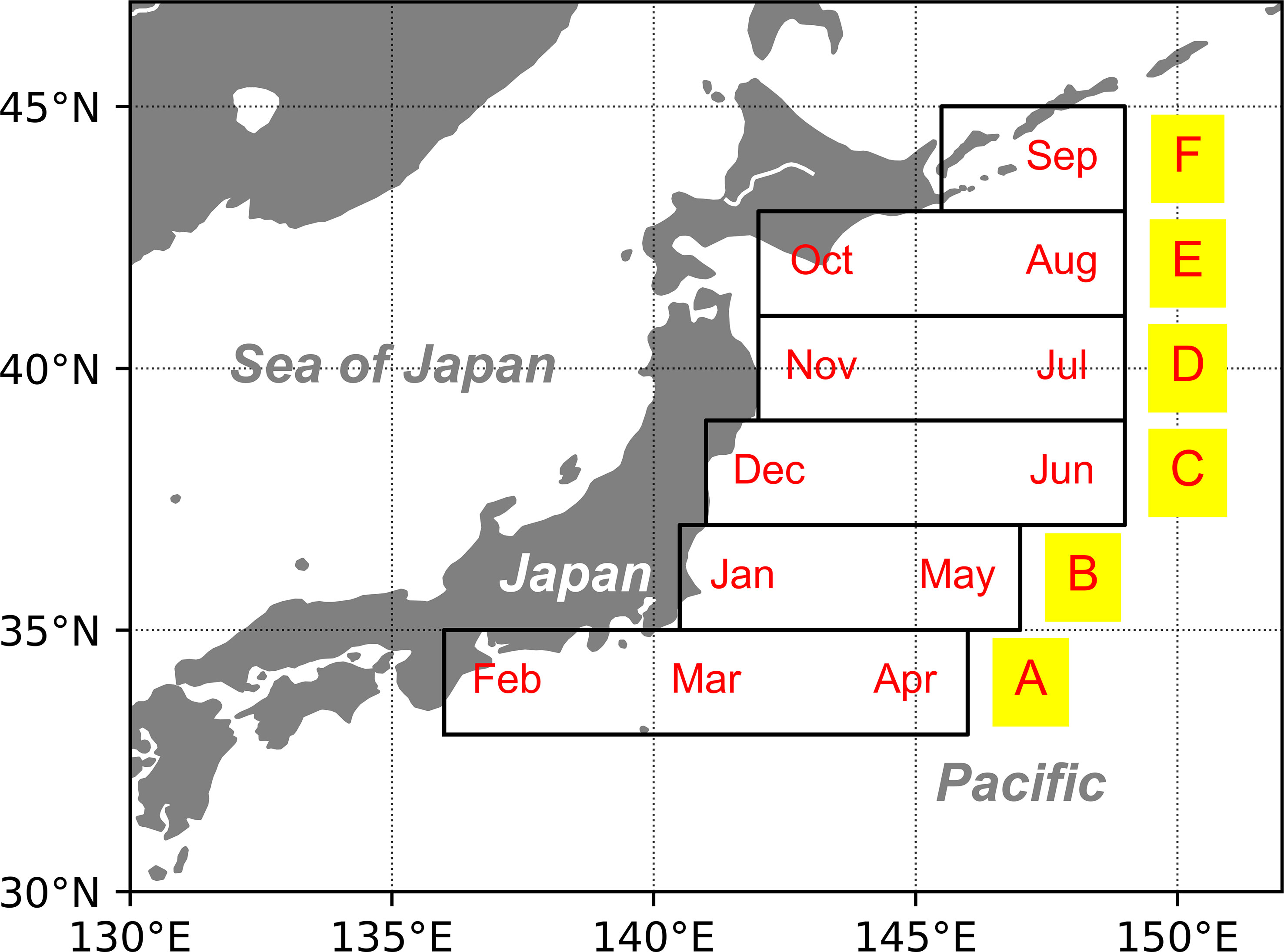
Figure 1 Spatial distribution of six boxes representing the ontogenetic migration of chub mackerel in each month (from south to north are A–F orderly). The distribution and migration of chub mackerel were defined based on Yukami et al. (2019).

TABLE 1

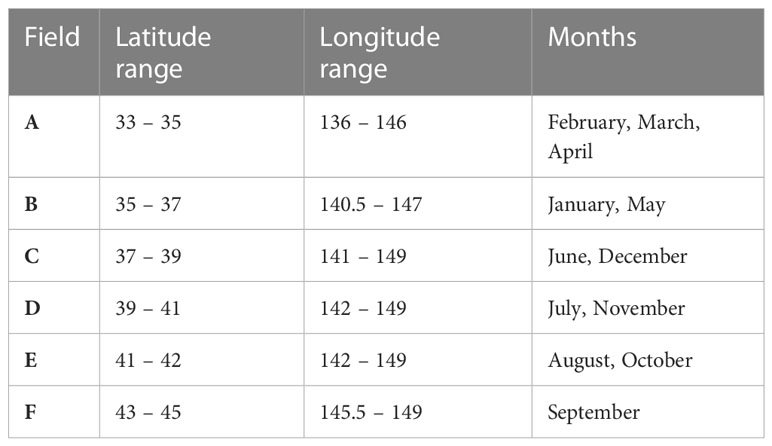
Table 1 The range of latitude and longitude of each employed box and the corresponding months of existence of chub mackerel.

TABLE 2

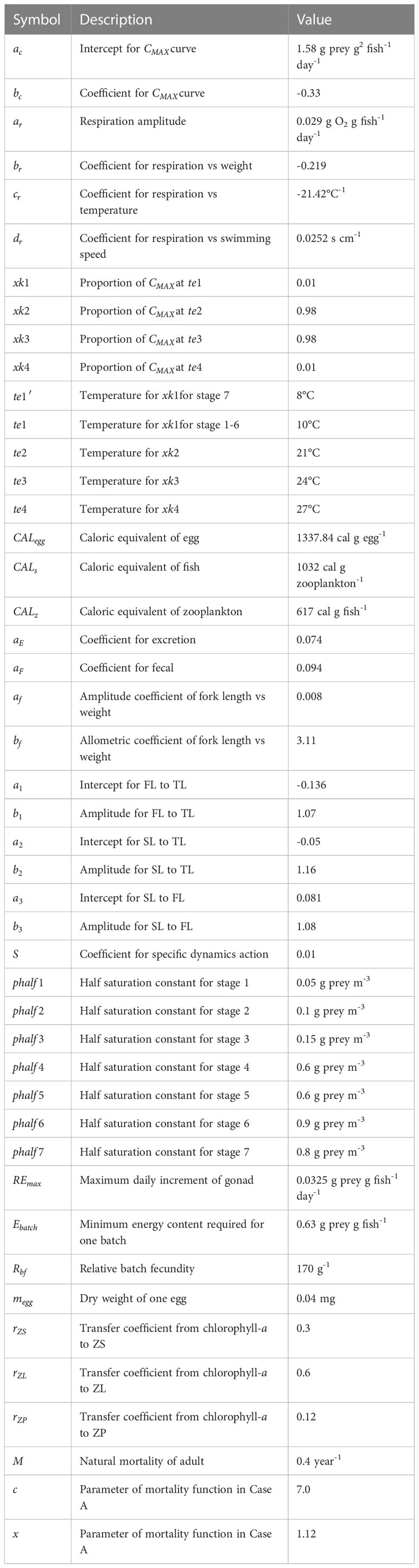
Table 2 Parameters employed in the model.

2.2 Bioenergetics model

To simulate the weight growth of individual chub mackerel, we extended the bioenergetics model of chub mackerel by Guo et al. (2022), which only targeted larval and early juvenile stages, to include full life cycles. The basic model is the Wisconsin bioenergetics model (Rudstam, 1988) (Eq. 1). The model simulated daily weight growth with half saturation constants as a function of standard length after the pre-larval stages. During the egg and pre-larval stages, we assumed that the model fish developed using energy from the yolk, as described later. The initial standard length and dry weight of chub mackerel in post-larvae were assumed to be 3.1 mm and 0.04 mg, respectively based on the findings of Hunter and Kimbrell (1980). Laboratory observations in the same study revealed that, first feeding occurred 46 hours after hatching and all larvae were observed to have fed by 60 hours after hatching (2.5 d). Metamorphosis occurred in 24 days at a standard length of 15 mm (Hunter and Kimbrell, 1980), which is regarded as the start of juvenile. In addition, fork lengths of 50 and 180 mm are regarded as the start of the young and immature stages of chub mackerel, respectively, according to field observations (Watanabe, 1970). The adult stage is assumed to be reached at an age of one year with a 288 mm fork length based on catch analysis (Hwang et al., 2008). Based on the above information, we divided the life stages of the chub mackerel, as shown in Table 3. The wet weight increment per unit weight of an individual was calculated according to the following equation:

TABLE 3

Table 3 Division of life history by days after being hatched and the sources.

$\begin{array}{ll}\begin{array}{c}\frac{1}{W}·\frac{dW}{dt}=[C-(R+E+F+SDA+\delta E_{buffer})]\frac{CA{L}_z}{CA{L}_f}\end{array}& (1)\end{array}$

where W is wet weight (g), C is consumption (g prey g fish^-1 day^-1), R is respiration (g prey g fish^-1 day^-1), E is excretion (g prey g fish^-1 day^-1), F is egestion (g prey g fish^-1 day^-1), SDA is a specific dynamic action (g prey g fish^-1 day^-1) or losses because of energy costs of digesting food, E_buffer is stored energy in the gonad for reproduction (g prey day^-1), δ is the Kronecker delta value, which is 1 when the fish releases the energy of reproduction stored in E_buffer; otherwise, the value of δ will be 0 (see section 2.3.1). CAL_z and CAL_f are the caloric equivalents of zooplankton (617 cal g zooplankton^-1 (Laurence, 1976)) and fish (1032 cal g fish^-1), (MEXT, 2015) respectively. The weight produced was transferred to the standard length (Eq. S21) as input to the population dynamics model to calculate the natural mortality.

2.2.1 Consumption

To estimate the maximum consumption curve as a function of weight, sufficient rearing experiments and field data are required. This study included both laboratory rearing experiments and field studies on stomach contents as references. The weight was then divided into a series of ranges to estimate the weight-specific average of C_MAX (Figure S2). Daily rations from the stomach content analysis from catch were multiplied by three times before being used because fish usually cannot predate enough in the natural field, and the parameters were then determined as an allometric function of wet weight (Wiff and Roa-Ureta, 2008; see Appendix). The post-larval stage is deemed to start predating on small zooplankton (ZS), and the juvenile stage is considered the start of feeding on large zooplankton (ZL) and predator zooplankton (ZP) (Castro and Hernandez-Garcia, 1995; Takagi et al., 2009). As there is no available data on zooplankton concentrations with the same resolution as in the model, the concentrations of ZS, ZL, and ZP were calculated from satellite-derived chlorophyll-a concentrations using pre-calculated ratios of chlorophyll-a to ZS, ZL, and ZP, respectively. The annual mean observed chlorophyll-a was calculated as 110 mg chlorophyll-a m^-3, which was based on assumption that ratio of carbon to chlorophyll-a is 60 (Batchelder and Miller 1989), with the annual mean observed biomass of phytoplankton 6.6 g C m^-3 (Kasai et al., 2001). The observed ZS, ZL and ZP were 3.2 g C m^-3, 6.6 g C m^-3 and 1.3 g C m^-3 in the same place, respectively (Yamaguchi et al., 2002; Ikeda et al., 2008). The zooplankton values were converted to 32, 66, and 13 g zooplankton m^-3 using 0.5 g carbon g dry-zooplankton^-1 (Omori, 1969) and 0.2 g dry-zooplankton g wet-zooplankton^-1. Then, the ratios of chlorophyll-a to concentrations of ZS, ZL and ZP were calculated as 0.3, 0.6 and 0.12 g zooplankton mg chlorophyll-a ^-1, respectively.

2.2.2 Dissipation terms

Oxygen consumption rate and respiration-related parameters were estimated for chub mackerel in the western North Pacific through laboratory-reared experiments (Guo et al., 2021), from which the value of parameter of swimming speed dependence d_r was calculated as 0.0252 s cm^-1, the parameter of mass dependence b_r was defined as -0.219, constant a_r and temperature dependence c_r were defined as 0.0290 g O₂ g fish^-1 day^-1 and -21.42°C, respectively (see Appendix). This study assumed chub mackerel swimming with an optimal speed U_opt in which the cost of transportation is the minimum. We used the same definition for U_opt with the highest limitation of 42.5 cm s^-1 in the respiration function with Guo et al. (2021). To avoid overestimation of respiration for smaller fish sizes by allometry fitting, we fixed b_r as 0 when the mass was smaller than 1 g. The dissipation terms of excretion and egestion followed the same equations as those used in a previous study (Ito et al., 2004). Energy partitioning experiments on juvenile chub mackerel in the laboratory revealed that 7.4% of total energy consumption was allocated to feces and 8.7% was allocated to the sum of urinary and branchial excretion. (Ohnishi et al., 2016). Therefore, the egesting coefficient of consumption a_F was assumed to be 0.074, and the excretion coefficient of consumption a_E was calculated as 0.094 according to a_E (1 – a_F) C = 0.087 C. Unfortunately, the energy partitioning rate of specific dynamic action has not been estimated for chub mackerel; therefore, we used the coefficient of SDA for Pacific herring (Megrey et al., 2007) for all stages since the post-larval stage of chub mackerel in this model. Because there is no energy intake until the post-larval stage, all energy losses (R, E, F and SDA) were fixed at 0 before the post-larval stage, with the assumption that all energy was transferred from the yolk sac to the larvae before the pre-larval stage.

2.3 Population dynamics model

The monthly cohort was employed to simulate population dynamics, as mentioned previously. The survival of monthly cohorts was calculated daily as follows:

$\begin{array}{ll}\begin{array}{c}\frac{d{N}_{m,y}}{dt}=N_{m,y}\times (-N_{mol}-F_{mol})\end{array}& (2)\end{array}$

where N_m,y represents the individual number of monthly cohorts in m month in y year, N_mol is the natural mortality, and F_mol is the fishing mortality. The annual age-specific fishing mortality coefficients of chub mackerel were obtained from the stock assessment report of the JFA (Yukami et al., 2019). The natural mortality from post-larval to the time chub mackerel reached 365 days of age was assumed as follows based on Bartsch and Coombs (2004):

$\begin{array}{ll}\begin{array}{c}{N}_{mol}=c\frac{G^{1-x}}{L^{1+x}}\end{array}& (3)\end{array}$

where c represents a magnitude of natural mortality, G means the daily growth rate of standard length, which was fixed as 0.63 mm day^-1 during the first year for simplification or calculated from bioenergetics model. The value of 0.63 mm day^-1 was estimated by a pre-calculated standard length 23 cm in 365 days after hatching in the bioenergetics model divided by 365 days. L is the standard length (mm), and x is the sensitivity parameter, which was adjusted together with c to minimize the difference between the model-derived results and observations (see details in Section 2.5). The natural mortality was defined as 0.4 year^-1 after 365 daily age (Honma et al., 1987).

As for the natural mortality of the egg stage, a laboratory experiment estimated it to be 10% per day (Lockwood and Nichols, 1977); however, the value did not include mortality by predation. Therefore, the mortality of the egg stage was assumed to be the same as the mortality on the first day of the pre-larval stage calculated by the mortality function (Eq. 3) to maintain the continuity of mortality function during the egg and larval stages. The period of the egg stage was calculated according to the function of the effective accumulated temperature (Watanabe, 1970) obtained from the laboratory as follows:

$\begin{array}{ll}\begin{array}{c}lo{g}_{10}H=\frac{4338.43}{K}-13.0702\end{array}& (4)\end{array}$

where H is the hours required for hatching, and K is the absolute temperature in Kelvin on the egg-spawned day.

2.3.1 Spawning algorithm

This study employed the structure of spawning algorithms developed for Atlantic mackerel (Gkanasos et al., 2019) with several modifications and parameter replacements for the applicability of chub mackerel (Figure 2). The spawning season was assumed to be from January to June, based on observations (Watanabe, 1970). We estimated the daily maximum energy (converted to weight of food in the model) that the gonad can store (RE_max) during the spawning season as:

FIGURE 2

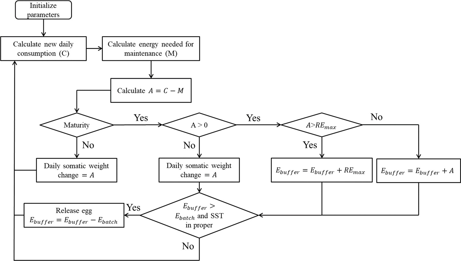
Figure 2 Overview of process of spawning algorithm in the bioenergetics model. RE_max defines daily maximum energy that the gonad can store (Eq. 5). E_buffer defines the current stored energy in gonad. E_batch defines the minimum weight of food required for a batch of eggs (Eq. 6).

$\begin{array}{ll}\begin{array}{c}R{E}_{max}=\frac{R_{bf}\times m_{egg}\times sex ratio\times \frac{CA{L}_{egg}}{CA{L}_z}}{Spawning interval}\end{array}& (5)\end{array}$

where R_bf is the relative batch fecundity set at 170 g^-1 (Yamada et al., 1998), the sex ratio of weight was assumed as 0.5, and the shortest spawning interval was assumed as one day (Table 3; Yamada et al., 1998). The mass of one egg m_egg was calculated by dividing 0.04 mg dry weight by the remaining water content of 76.6% (Valdes Szeinfeld, 1993): 0.04/(1 – 76.6%) = 0.17 mg. RE_max was calculated to be 0.0325 g prey g fish^-1 day^-1. If the net energy from food intake was higher than RE_max, RE_max was added to the stored energy in the gonad (E_buffer). Otherwise, all net energy intake was stored in the gonad, unless the net energy intake became negative.

The minimum weight of food required for a batch of eggs (E_batch) was calculated using Eqs. 6 and 7:

$\begin{array}{ll}\begin{array}{c}{E}_{batch}=E_0\times R_{bf}\times \frac{1}{CA{L}_z}\end{array}& (6)\end{array}$

$\begin{array}{ll}\begin{array}{c}{E}_0=m_{egg}\times CA{L}_{egg}\end{array}& (7)\end{array}$

Where E₀ means energy content of one egg and CAL_egg represents caloric equivalent of egg, which was assumed as 1337.84 Cal g egg^-1 based on Valdes Szeinfeld (1993) (transformed from joule 5600 J g egg^-1). E_batch was calculated to be 0.063 g prey g fish^-1. The optimal temperature for spawning is 16–20°C (Okabe et al., 2012). Therefore, 16°C was set as the lowest spawning temperature in the spawning algorithm. When SST was appropriate and E_buffer was larger than E_batch, the cohort spawned a new batch of eggs. The total number of spawned eggs during a specific month was integrated and released into the model at the end of the month to produce the new monthly cohort.

2.4 Initialization and simulation

Before each simulation, the model was spun up for 20 years to reach the equilibrium stage under the monthly average climatological condition calculated by:

$\begin{array}{ll}\begin{array}{c}{\overline{var}}_m=\frac{{\sum }_{1998}^{2018}va{r}_{m,y}}{21}\end{array}& (8)\end{array}$

where var is the SST or concentration of prey zooplankton and m and y represent the month and year ranges, respectively (See in Figure S1). The average fishing mortality coefficients were also used during the spin-up process. At the start of the spin-up run, the age structure of the chub mackerel in 1998 was used as the initial condition. The steady state showed a stable trend and there is no overshooting or collapse of stock, that means the model is stable (Figure S3).

2.5 Evaluation of model skill

To evaluate the model performance, the root-mean-square error (RMSE) was employed for the biomass and RPS. However, because the distribution of observed biomass and RPS were not normally distributed, as reported by JFA (Yukami et al., 2019), the values were log-transformed. In addition, because the units between the biomass and RPS are different, standardized anomalies were calculated by dividing the anomalies from the average by the standard deviation. The combined RMSE is then calculated as λ:

$\begin{array}{ll}\begin{array}{c}\lambda =\sqrt{RMS{E}_{biomass}^2+RMS{E}_{RPS}^2}\end{array}& (9)\end{array}$

where RMSE_biomass and RMSE_RPS are the RMSEs of the log-transformed normalized anomaly of biomass and RPS (abbreviated as LTBIO and LTRPS hereafter), respectively. To calculate λ, data from 1998 to 2014 were used because the accuracy of RPS might be lower after 2014 due to lack of data to estimate RPS using a virtual population dynamics model. Indeed, the RPS data in the last six years have been frequently revised in the stock assessment report of the JFA. The mortality parameters c and x varied from 4.0–8.0 and 0.0–4.0, respectively. The combination of c and x showed that the minimum λ was selected for each case study, as shown in Section 2.6.

2.6 Experimental plan

All numerical experiments are listed in Table 4. In the control run (Case A), mortality was calculated using a fixed daily growth rate, whereas actual growth was calculated in the bioenergetics model (Table 4). In Case G, the mortality was calculated based on the daily growth rate derived from the bioenergetic model. By comparing the results of Cases A and G, the mortality dependence on size and growth was discussed.

TABLE 4

Table 4 Case studies in numerical experiments.

To clarify the mechanism by which environmental factors affect body growth and subsequent population dynamics, Cases C and T were carried out. Climatological SST was used in Case C to evaluate the effects of the interannual variation in prey zooplankton availability. Climatological chlorophyll-a was used in Case T to evaluate the effects of the interannual SST variability.

Additionally, the influence of fishing pressure was tested using three different fishing scenarios: low fishing pressure (Case LF), middle fishing pressure (Case MF) and high fishing pressure (Case HF). In Case MF, the interannual variations in fishing mortality coefficients were removed with the averaged fishing mortality coefficients from 1998 to 2018 for each age group (Table 5). Case-LF and Case-HF used fishing mortality coefficients by adding and subtracting the standard deviation of fishing mortality coefficients to the average, respectively. In further attempts to figure out how fishing pressure impact by age groups influences on the stock fluctuation, two sub-cases were conducted in Case-LF and Case-HF, respectively: Case-LF-0 which subtracted the standard deviation of fishing mortality coefficient only for age-0 group, Case-LF-1 which subtracted it for adult groups, Case-HF-0 which added it only for age-0 group, and Case-HF-1 which added it for adult groups. The above sub-cases allow us to determine the differences in degree of impact of fishing pressure to spawners or recruits.

TABLE 5

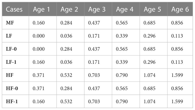
Table 5 Fishing mortality coefficients for each age group in the low-, middle-, and high-pressure case studies and their sub-cases.

3 Results

3.1 Modeled growth and life cycle

The average weight of survival cohorts of the same daily age from all monthly cohorts during 1998–2018 in Case A showed relatively rapid growth during age-1 (Figure 3). As a result, the model average overestimated the weight compared with the observation from age-2 to age-4. However, the observed values were within the 90 percentiles. In addition, the weight of age-0, which influences mortality in the model, was reasonably reproduced in Case A. The larvae mostly hatched from egg in 2–3 days and most metamorphosis occurred in 28 days in the model (Figure 4). Compared with observations that the eggs hatched in 56 hours at 19°C and metamorphosis occurred in 24 days at 16.8°C and 16 days at 22.1°C, the simulated hatch days of cohorts were fit with observations and simulated data of metamorphosis were slightly later than the observed days (Hunter and Kimbrell, 1980). The stages of life history were defined by the SL in the model, which was plotted as a black line in Figure 4, accompanied by the critical SL at the start of juvenile and young stages. The weight showed a peak in the fall for all age groups when they migrated back from the feeding ground in the model (Figure 5). The seasonal variation in the condition factor of chub mackerel on the Pacific coast was reported to show its peak in fall and winter (Yatsu et al., 2019), which was consistent with the model results.

FIGURE 3

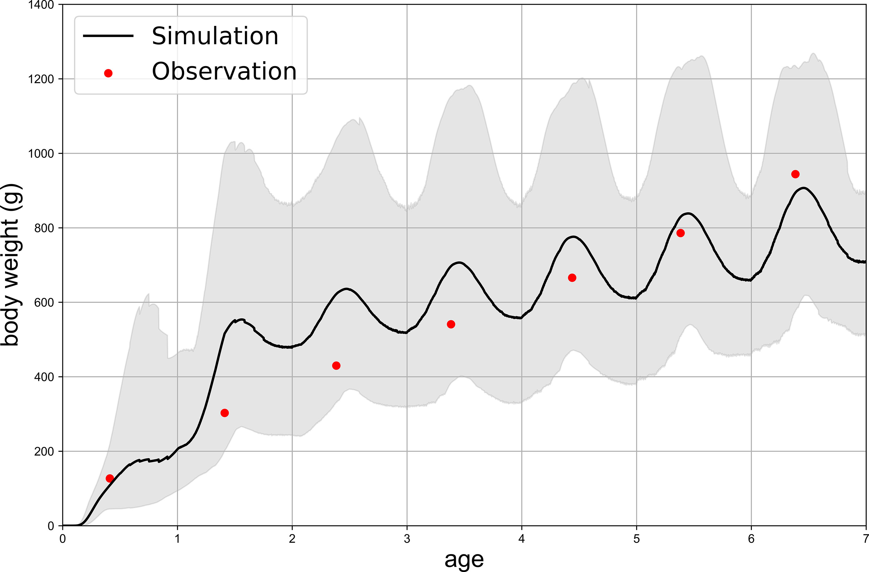
Figure 3 Weight variations simulated in Case A. Black line represents the average weight among all monthly cohorts in each day while the upper and lower boundary of grey field indicate the highest and lowest 10% of the total cohorts, respectively. Red points are observation data from Yukami et al. (2019).

FIGURE 4

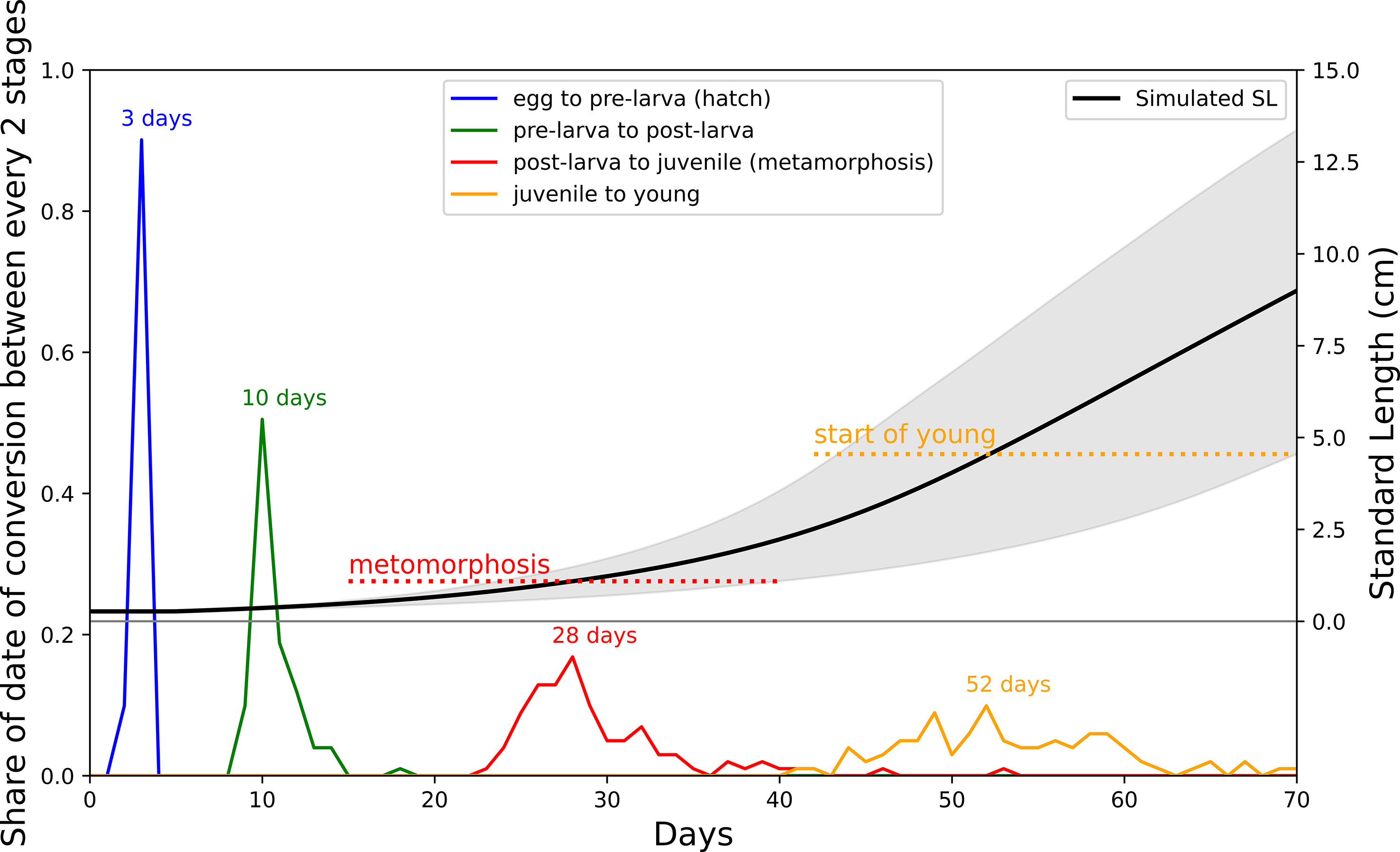
Figure 4 Distribution of frequency of starting date of each stage. Blue line is starting date of pre-larval with peak in three days; Green line is starting date of post-larval with peak in 10 days; Red line is start date of juvenile (metamorphosis) with peak in 28 days; Yellow line is start date of young with peak in 52 days. Black line represents simulated SL growth while grey field is 90 percentiles. Dashed red line and yellow line denotes critical SL for juvenile and young respectively.

FIGURE 5

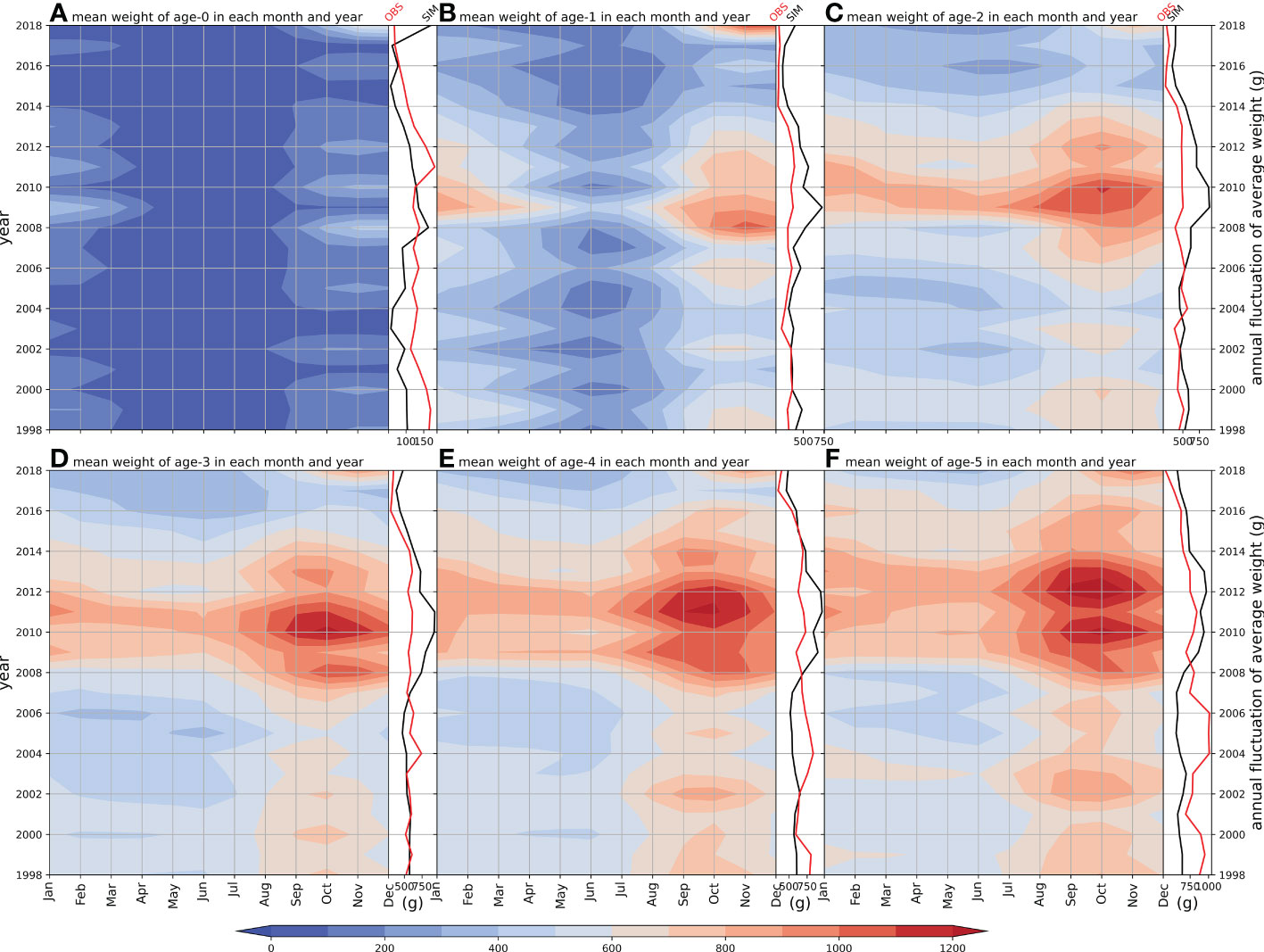
Figure 5 Hovmöller diagram of simulated age-specific mean weight and age-specific weight of annual fluctuation (black line) compared with observation (red line), (A–F) illustrate age 0–5 groups respectively.

The first reproduction started in 368 days and was mostly distributed during 368–383 days in the model (Figure 6A). The cohorts whose first reproduction occurred in age-1 occupied 74% (75/101) of the total cohorts, while the cohorts whose first reproduction occurred in age-2 occupied 26% (26/101) of the total cohorts (Figure 6A). The abundance of spawning eggs peaked from March to June in the model (Figures 6B–G), which almost corresponded with the survey on chub mackerel (Yukami et al., 2019). The principal spawners were age-1,2,3 groups because of the large group size, while the elder groups spawned at a higher frequency than the younger groups (Figures 6B–H).

FIGURE 6

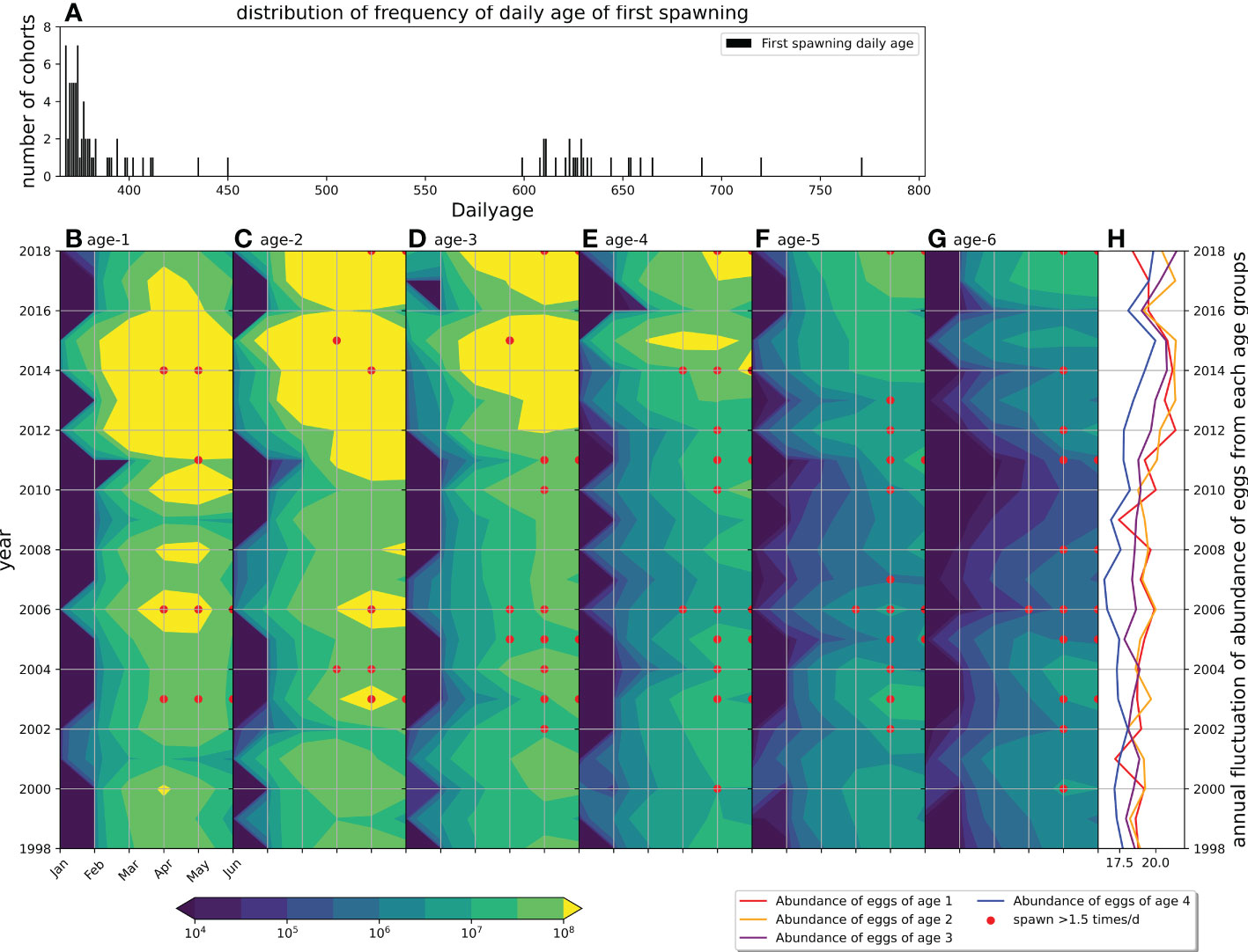
Figure 6 Distribution of frequency of date of first reproduction of all projected monthly cohorts (A). Hovmöller diagram of abundance of spawned eggs from age-specific spawners groups (B–G represents age 1–6 spawners respectively). Points denote the frequency of spawning where red point denotes the cohort spawns more than 1.5 times every day. Lines with colors (H) represent annual fluctuations of abundance of eggs from age-1 (red), age-2 (yellow), age-3 (purple) and age-4 (blue).

3.2 Modeled biomass and RPS fluctuations

The annual fluctuation of the modeled weight of age-0 peaked around 2008 and decrease during 2001–2007, which was similar to the observation with a lag of a few years (Yukami et al., 2019) (Figure 5). The modeled weights of other age classes were overestimated compared with the observations, but a decreasing trend since 2012 was captured (Figures 5B–F).

The annual fluctuation in the abundance of spawning eggs showed an increasing trend during 2009–2015 (Figures 6B–H). To separate the influence of the size of spawner group, the spawning frequency was scattered in the corresponding months, from which we found that the spawning frequencies were high before 2009 and after 2009 for age-1 to age-6 groups as the red dots in Figures 6B–G, which represent the spawner spawned more than 1.5 times every day, respectively (Figures 6B–G). The survival of age-0 was defined as S365 (survival rate in 365 days) in the model that was scattered corresponding to the experienced SST and chlorophyll-a in the first month by using the monthly cohorts, from which S365 was found to be high from April to June (Figure 7). Eleven strong monthly cohorts were identified in Case A using the definition that S365 was higher than the average plus one standard deviation (Figure 7). The strong cohorts were mainly caused by good prey conditions in June 2002, April and May 2004, June 2008, and May 2010, and by a short duration of egg period with warmer SST in April 1998, May and June 2000, June 2010, June 2014, and June 2017 (Figure 7).

FIGURE 7

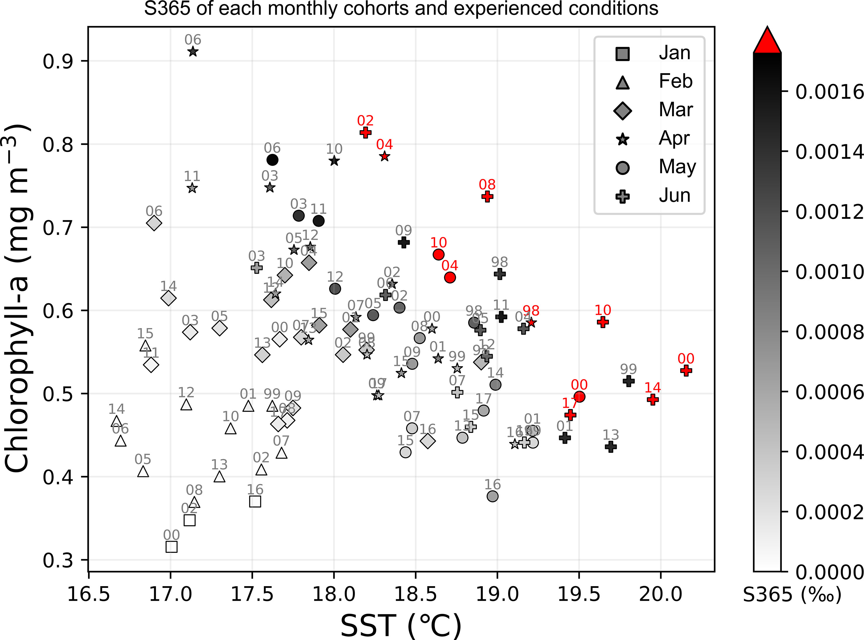
Figure 7 Distribution of survival rate at 365 days after being hatched (S365) of all the simulated cohorts in Case A on the experienced SST and chlorophyll-a (experienced in the first month) plane. Various markers indicate the different months while the color bar represents the value of S365 (unit is ‰), where the red color means the survival rate is higher than average plus standard deviation, which also could be called as strong cohort.

The model reproduced the increasing trend of abundance and biomass from 1998 to 2018 in Case A (Figure 8, normalized anomalies for logarithm are in Figure S4). Both observed RPS showed strong year classes in 2002 and 2004. The model RPS amplitudes were not sufficient, but revealed relatively higher values in 2002 and 2004. The observed biomass increased after 2009, and the model also showed a biomass increase during the same period. Although the rapid increase in biomass after 2013 was not reproduced in the model, the combined RMSE λ (Eq. 9), were not evaluated after 2012. The distribution of λ showed a higher dependency on x (length dependency parameter of mortality) than c (growth dependency parameter of mortality). The optimal combinations of x and c were found to be x = 1.12 and c = 7.0, respectively, in Case A with λ = 1.40. The resulting number of natural deaths in the age 0 cohort was much higher than the number of deaths from fishing (see Figure S5, where the black bar is invisibly small), indicating the importance of natural mortality.

FIGURE 8

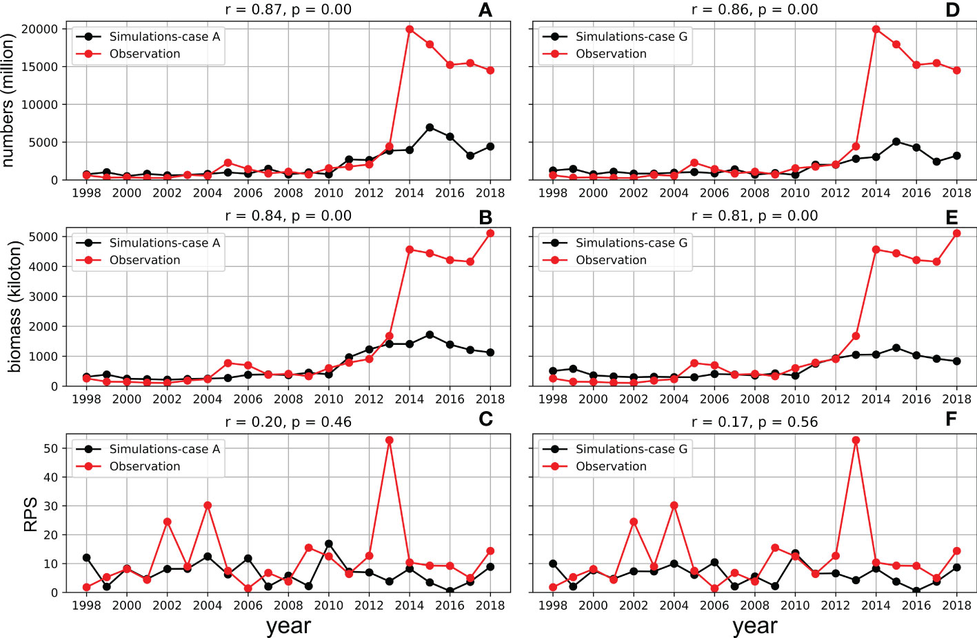
Figure 8 Simulated (black lines) and observed (red lines) abundance of adult individuals (upper, A-Case A; D-Case G), biomass (middle, B-Case A; E-Case G) and RPS (bottom, C-Case A; F-Case G) of whole cohorts from 1998 to 2018 in Case A (left) and Case G (right). The observed values were from Yukami et al. (2019).

3.3 Growth effects on mortality

The pattern of the distribution of λ in Case G, in which the growth estimated by the bioenergetics model was used to calculate natural mortality, was different from that in Case A. The dependency on c (growth dependency parameter of mortality) increased and became comparable with x (length dependency parameter of mortality) in the range x was between 0.1 and 2.2 in Case G (Figure 9B). For a given c, although there is only one minimum value of λ in Case A, there are two local minimum values of λ in Case G (Figure 9) across x = 0.9. When x is greater than 1, natural mortality decreases with an increase in growth. When x is lesser than 1, natural mortality increases with an increase in growth. The minimum λ (= 1.45) was obtained with c = 6.5 and x = 0.905 in Case G, in which higher growth contributes to higher natural mortality. In addition, the minimum λ (= 1.45 with c = 6.5, x = 0.905) in Case G was larger than the minimum λ (= 1.40, with c = 7.0, x = 1.12) in Case A (Figure 9), which suggests the importance of the size-dependency of natural mortality in reproducing realistic stock increases in chub mackerel. Indeed, the abundance and biomass produced in Case A showed higher correlation coefficients than those in Case G (Figures 8D, E). However, the simulated RPS in Case G showed a higher sensitivity and produced a higher correlation coefficient with the observation than in Case A. A more dramatic increase was remarkable, especially in 2002 and 2004, when the observed RPS showed strong year classes (Figure 8F), which may indicate the importance of the growth dependency of natural mortality in projecting the RPS.

FIGURE 9

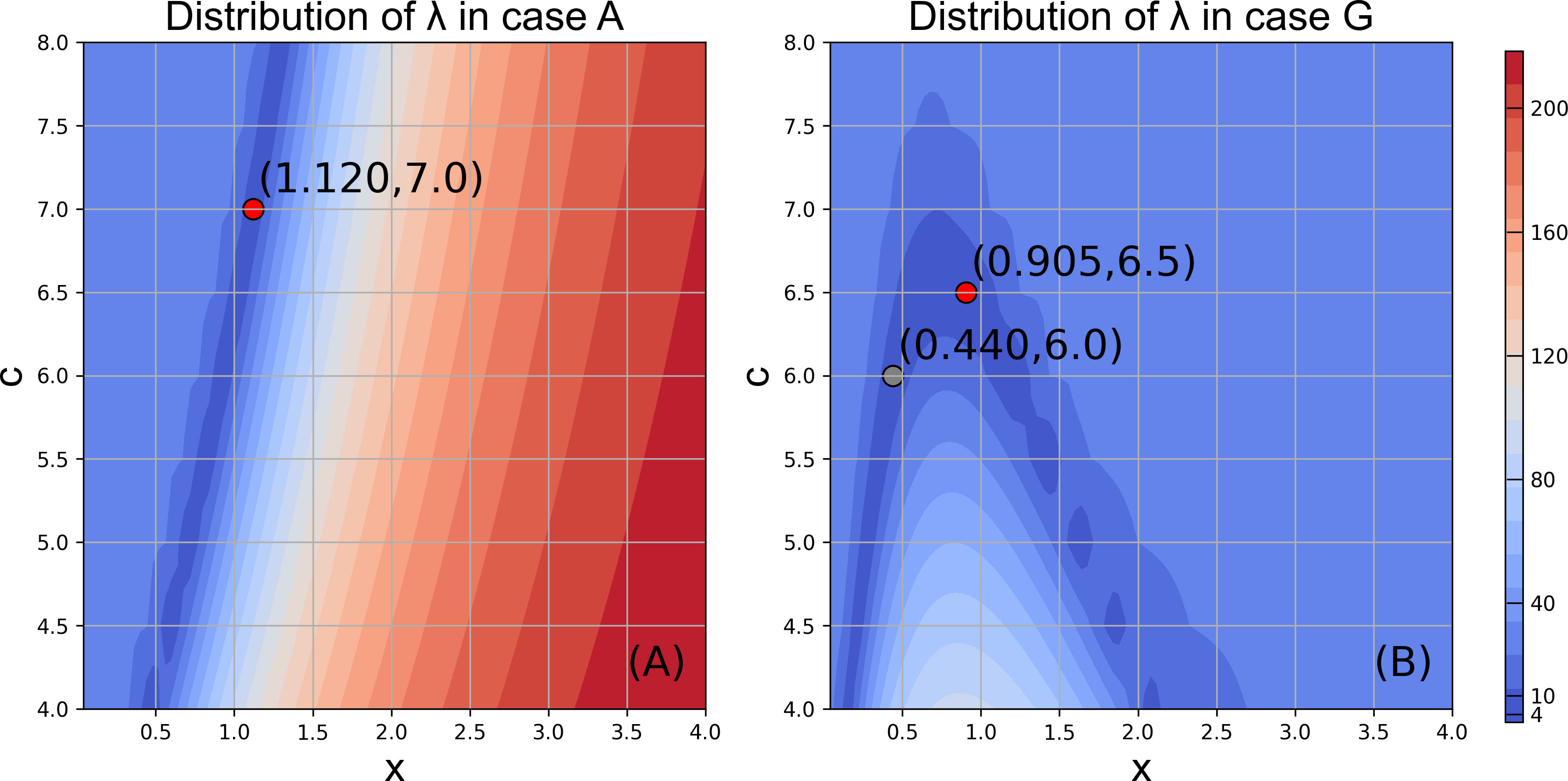
Figure 9 Distribution of λ in Case A (A) and Case G (B) in the given ranges of x and c. Red points represent the minimum value in the limited plate respectively, which indicates the best performance of model. Grey point in (B) denotes the local minimum value.

3.4 Environmental effects on survival

In Case C, in which climatological SST was used as the forcing, the biomass increase pattern was very similar to that of Case A (Figure 10). Even for RPS, the interannual patterns were similar between Case C and Case A. By contrast, the biomass trends and RPS fluctuations were relatively different in Case T, in which climatological prey zooplankton concentrations were used as the forcing, with those of Cases A and C. However, the biomass increased after 2014. Meanwhile, the comparison also shows that SST is the principal driver for the increasing trend of stock after 2013 in Case T, which corresponds well to the rapid increase in observed biomass after 2014.

FIGURE 10

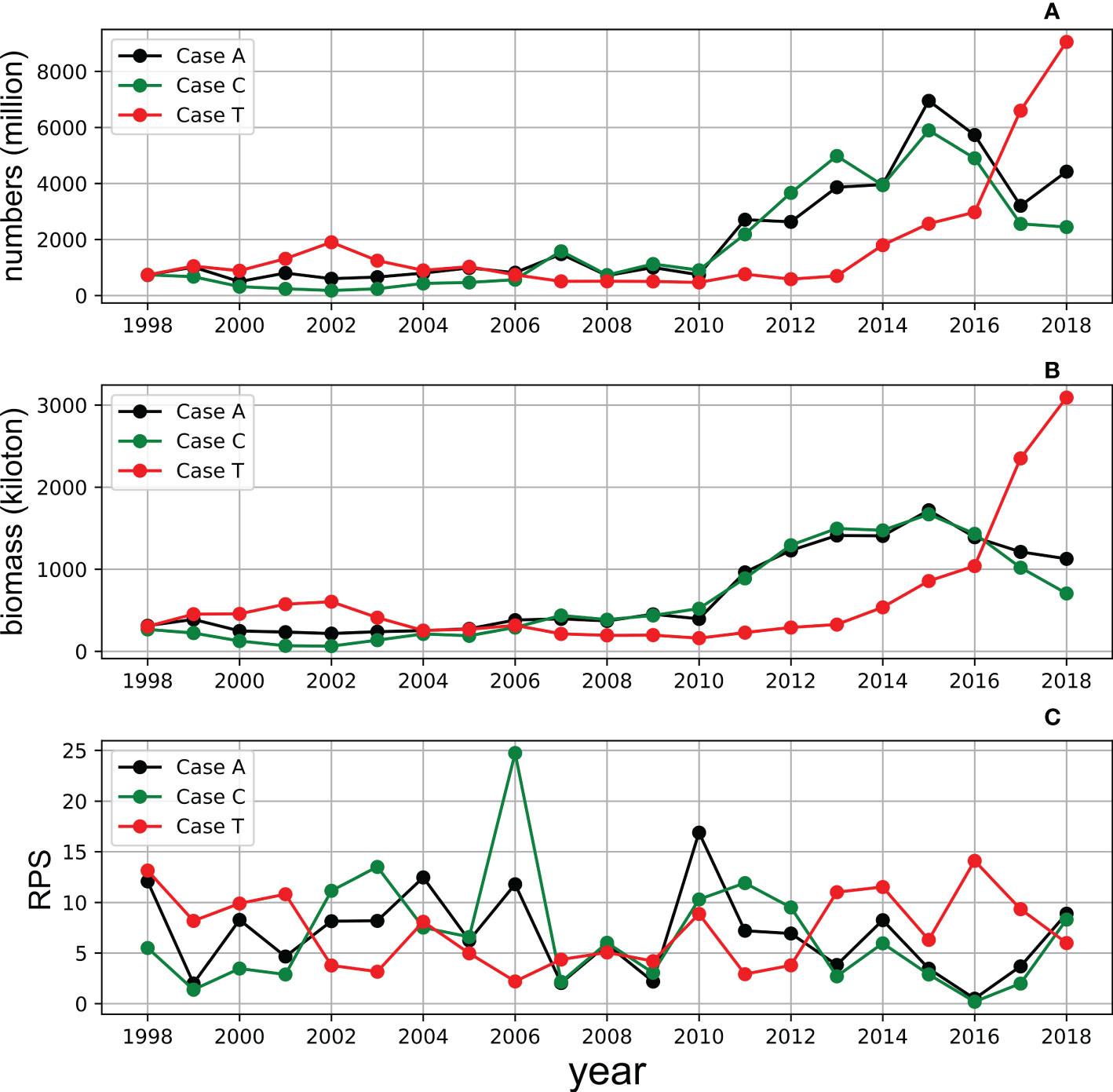
Figure 10 Simulation of the annual adult numbers (upper, A), biomass (middle, B) and RPS (bottom, C) of whole cohorts from 1998 to 2018 in Case A (black), Case C (green) and Case T (red).

3.5 Effects of fishing pressures

The population of chub mackerel showed a rapid increase after 2010 with moderate fishing pressure (Case MF, Figure 11B), which was similar to Case A (Figure 8A). However, the surviving population was much higher in Case MF than that in Case A. For example, the surviving adult population exceeded 5,000 million in 2011 in Case MF, but it occurred in 2015 in Case A. The maximum surviving adult population surpassed 10,000 million in 2015 in Case MF, whereas it was less than 7,500 million in Case A. The population of chub mackerel also showed a rapid increase after 2010 with low fishing pressure (Case LF, Figure 11A). In contrast, the population of chub mackerel decreased under high fishing pressure (Case HF, Figure 11C). The influence of fishing pressure on the biomass was larger when the fishing pressure on spawners was enhanced or weakened compared with the case when the fishing pressure on recruits was enhanced or weakened (Figure 12).

FIGURE 11

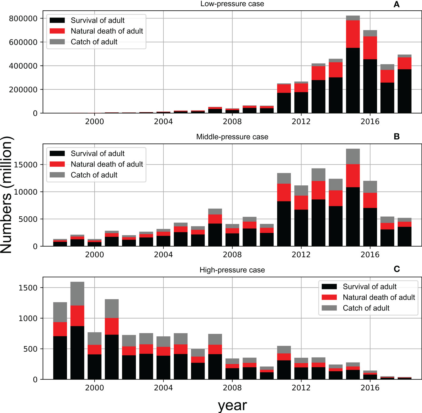
Figure 11 Simulated survival (black column), natural death (red column) and catch (grey column) of adult in low-pressure case (upper, A), middle-pressure case (center, B) and high-pressure case (bottom, C). The stacked bar denotes the total population without any death while the red and grey bar represent the different causes of death.

FIGURE 12

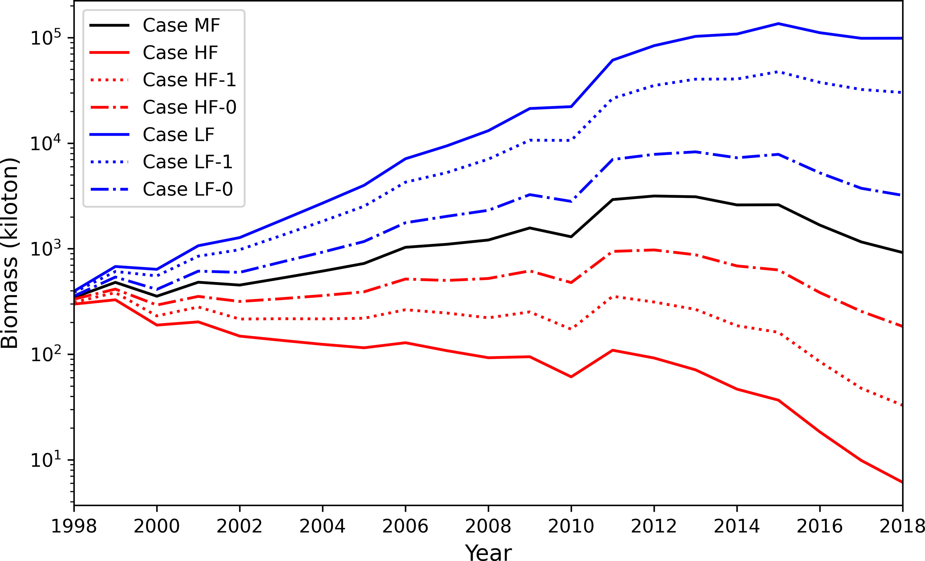
Figure 12 Plots of biomass in the simulation of Cases MF (averaged fishing pressure), HF (increased fishing pressure) and LF (decreased fishing pressure) and their sub-cases. Black line is Case MF, blue line is Case LF and red line is Case HF; Dotted lines denote sub-cases in which the fishing pressure was increased/decreased only for adults while dot-dashed lines denote sub-cases in which the fishing pressure was increased/decreased only for recruits.

4 Discussion

This study built up a bioenergetics and population dynamics coupled model with the whole life history of chub mackerel, which is the first study to analyze the population dynamics from a comprehensive perspective including feeding energy intake and energy dissipation; hence, temperature and food availability influence growth, reproduction process, ontogenetic migration, size/growth-dependent mortality, and fishing pressure. Using this model, the daily mortality rate, which is difficult to measure from field data, could be estimated based on simulated daily body growth and, hence, the size of fish. The model used a simplified representation of the ontogenetic migration of chub mackerel. However, analyzing the survival and stock fluctuation mechanisms of chub mackerel in terms of monthly cohorts could provide a more detailed understanding of the impact of environmental factors on these processes.

4.1 Mortality function

Bartsch and Coombs (2004) proposed the growth- and length-dependent mortality of Atlantic mackerel. We used the same type of function for natural mortality, but compared two cases: a fixed growth case and a daily growth rate case estimated from the bioenergetics model. The optimal dependency parameters were identified by changing the mortality dependency on growth/size (x) and the mortality amplitude (c). The distribution of λ exhibited a higher dependency on x than c in Case A. This can be expected because the growth rate was fixed when the natural mortality was calculated in Case A. Indeed, the dependency on c increased and became comparable to x in Case G. The minimum λ was obtained with x larger than 1, and the natural mortality increased with length, but was compensated by a decrease with an increase in growth in Case G. In Bartsch and Coombs (2004), the original value of x and c for Atlantic mackerel was 0.3 and 5.0, respectively, which indicates an increasing mortality with increase of growth. In this case, the influencing pattern of growth dependency is different from that of the chub mackerel in this study.

The minimum λ was smaller in Case A than that in Case G, suggesting that it is not necessary for the model to employ the simulated daily growth rate for the mortality function. However, this does not deny the importance of the daily growth rate. The daily growth rate influences the length of fish and subsequently, the natural mortality (Eq. 3). Notably, the egg mortality depends not only on Eq. 3, but also on the duration of egg periods, which determines the survival rate at 365 days after hatching (S365) to a considerable degree and subsequently the performance of the model. On average, the number of deaths during the egg stage accounted for 97.1% of the total number of deaths until 365 days of age in Case A. The egg-stage duration becomes longer when the temperature is cooler, and cooler temperatures also influence slower growth of larvae. Egg mortality may partially compensate for the effect of growth on natural mortality.

Note that the density-dependent effect is not included in the current model. Density dependence on growth and body condition was observed in chub mackerel (Kamimura et al., 2021). To incorporate the density dependence of food availability, a dynamic linkage between prey food and fish predation should be included (Rose et al., 2015), in which prey concentration is changed by predation pressure from fish. In this study, we used satellite-derived prey zooplankton concentrations, and it was impossible to include dynamic linkage, but it is possible to couple with a lower trophic ecosystem model (Ito et al., 2004). By including density dependence, the length and growth dependency of natural mortality might change. This should be investigated further in future studies.

4.2 Stock fluctuations

The coupled model in this study successfully captured the increasing trend of the stock of chub mackerel from 1998 to 2018 (Figure 8). The monthly cohorts were used in the model. The high survival rate cohorts, also called as strong cohorts, have contributed to an increase in the population. Strong monthly cohorts occurred when the larvae experienced higher SST and/or higher chlorophyll-a concentrations (Figure 7). The chlorophyll-a concentration showed significant positive correlations with S365 (Figure 13, p< 0.05, for the February, March, April, and May cohorts) by controlling net food intake (Figure S6-1&2, p< 0.05, for all monthly cohorts). These results suggest that prey availability is one of the most important drivers of stock fluctuation. However, there were outliers that showed higher S365 values than others in the same chlorophyll-a range. Outliers were frequently observed in June, which seemed to decrease the correlation between chlorophyll-a and S365 in June. The outliners experienced warmer temperatures higher than 19.4°C (Figure 7). The egg stage is the period with the highest natural mortality rate during the whole life stage, and even a small change in duration may cause a great difference in survival after one year.

FIGURE 13

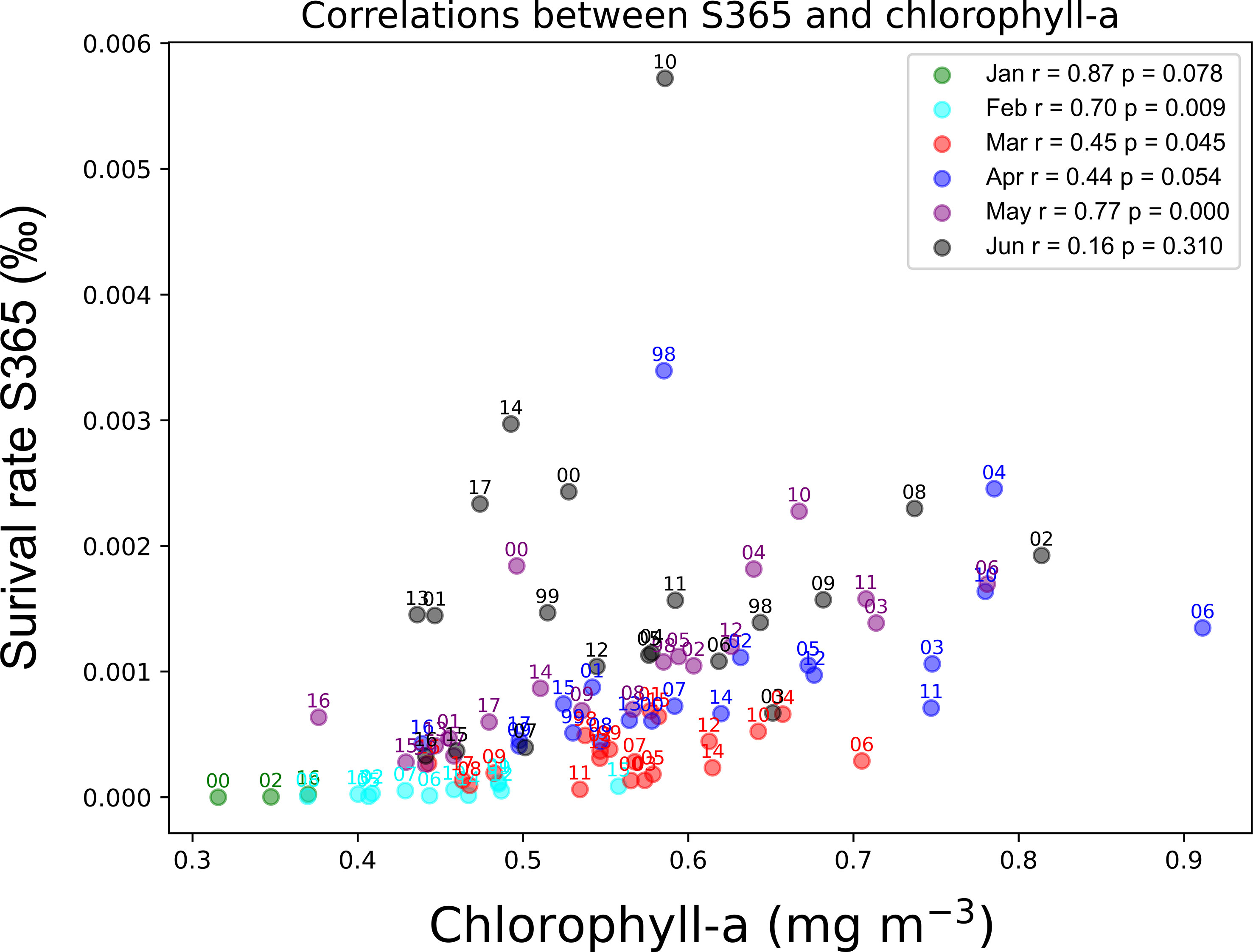
Figure 13 Scatters which show the correlations between S365 and experienced chlorophyll-a during the first month of each monthly cohort. Colors represent cohorts in different months while the numbers beyond the circles mean the year. Correlation coefficient r and its p-value shown in legend are calculated in monthly-specific.

The different environmental influences on stock fluctuations can be recognized by comparing case studies. The increasing trends in the population in Case C seem to be similar to those in Case A, which suggests a strong influence of chlorophyll-a in Case A. Before 2010, when the prey availability-induced strong cohorts frequently occurred, the population fluctuations were similar in Cases A and C. After 2010, when warmer SST frequently induced strong cohorts, the population difference between Case A and Case C increased. Simultaneously, the population increased rapidly in Case T. The results suggest the contribution of prey availability to the increasing trend before 2010 and the contribution of SST after 2010. Environmental influences also show seasonal differences. Kaneko et al. (2019) analyzed the correlation between temperature and RPS seasonally and confirmed the negative impact in winter in spawning ground and positive impact in nursery ground, indicating a seasonal difference in the impact of SST. The correlation between temperature during the spawning period (January to June) and annual LTRPS was significantly negative in this study (Figure 14A, r = -0.46, p = 0.03), which emphasizes the importance of temperature in the spawning period on LTRPS. However, the temperature from July to December did not show a significant impact on LTRPS (Figure 14A, r = -0.03, p = 0.89), which implies seasonal differences in the influence of SST, which may be attributed to different stages of life history. Meanwhile, chlorophyll-a showed a more significant correlation with LTRPS based on the model in this study, not only in the spawning period, but also in the first year (Figure 14B), where a profound impact from food supply can be figured out. Annual population dynamics were projected for chub mackerel during 1976–2000 with different temperature scenarios in Suda et al. (2008) wherein an increasing SST resulted in a lower stock, but seasonal differences in SST impacts and SST impacts on the spawning process were not considered. Our results indicate a clearer mechanism of SST impact on chub mackerel.

FIGURE 14

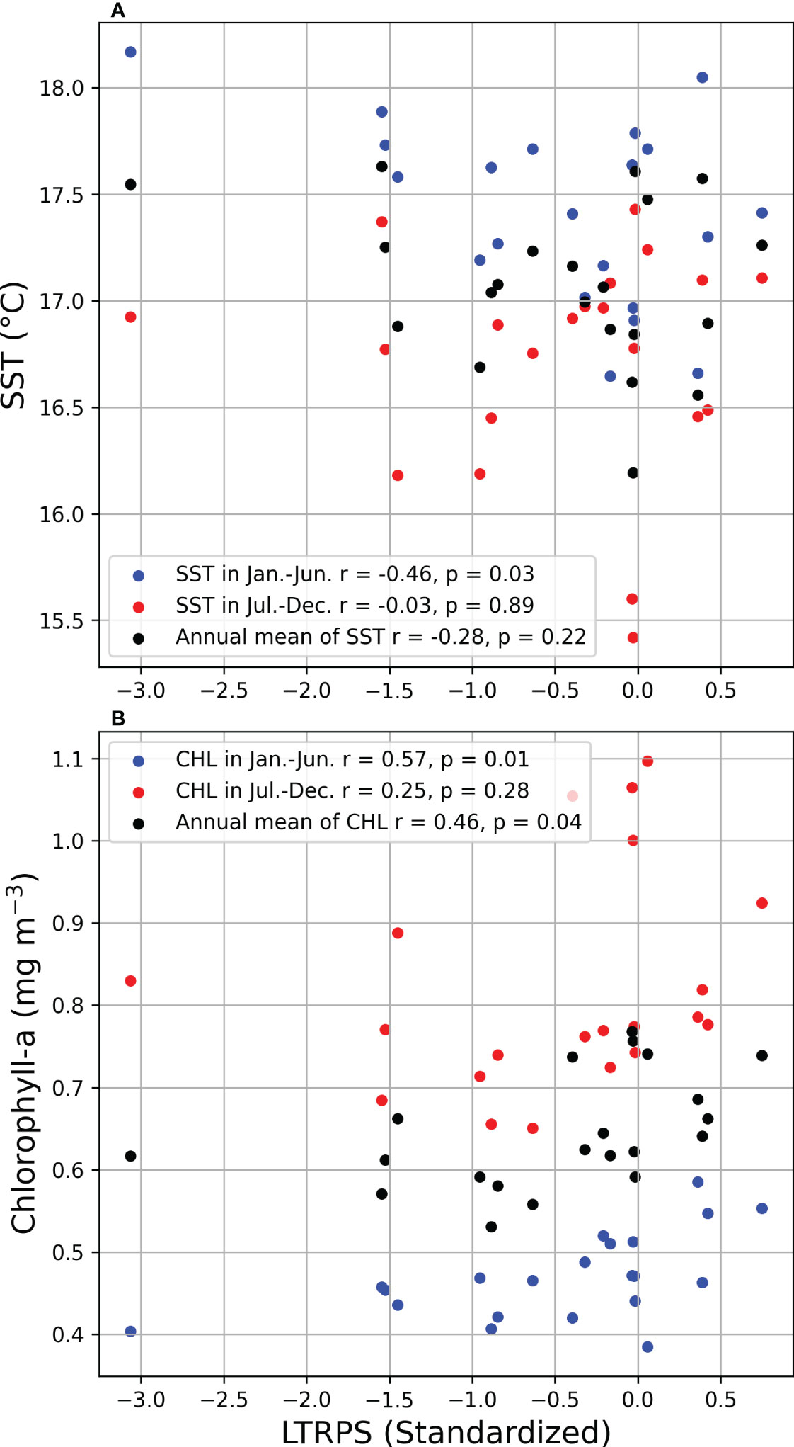
Figure 14 Correlation between log-transformed RPS (standardized) and month-division SST (upper, A)/Chlorophyll-a (lower, B). Red, blue and black denotes the mean SST/Chlorophyll-a during Jan. to Jun., Jul. to Dec. and whole year respectively. Correlation coefficient r and its p-value shown in legends are calculated in different durations.

It was also noted that good prey availability or a short duration of the egg period is not sufficient for a strong cohort. For instance, the monthly cohort of April 2006 experienced extremely high chlorophyll-a over 0.9 mg m^-3 but suffered from a relatively cooler SST during its first year, and the monthly cohorts of June 2001 and 2013 experienced a warmer SST in the early life stage, while the supply of food was not suitable for growth (Figure 7). No strong cohorts appeared in any of the three cases. It seems that the thresholds in both environmental factors SST and chlorophyll-a exist around 18.3°C and 0.46 mg m^-3 respectively, below which strong cohorts are not expected. The 18.3°C is close to the threshold temperature indicated by Kamimura et al. (2015), during which there is a significant correlation between the growth rate and SST. Another significant correlation between RPS and experienced temperature was determined over 5–11 April from 2001–2012 in a particle experiments correlation that depicted a shifting axis of Kuroshio induced different peaks of experienced temperature (Kaneko et al., 2019). The experienced temperature will be over 18°C if the axis of the Kuroshio is closer to the spawning ground, resulting in a higher RPS (Kaneko et al., 2019).

Additionally, fishing pressure affects the occurrence of strong cohorts. For example, SST and chlorophyll-a satisfied the conditions that could generate a strong cohort, but the resulting S365 value was not high (Figure 7). When the fishing mortality coefficients changed to the averaged during 1998–2018 for each age group (Table 4, as the same as Case MF), the monthly cohort in June 1999 became a strong cohort (Figure S7). This change suggests that fishing pressure can also become an obstacle for producing strong cohorts besides SST and chlorophyll-a, which are the principal drivers of stock fluctuations. The trajectory of survival rate of June 1999 cohort in Cases A showed a steeper decrease of survival rate than that in Case MF because of higher fishing pressure in Case A than Case MF (See in Figure S8). The importance of fishing pressure was also confirmed through case studies with different fishing pressures. Under the high fishing pressure scenario, the increasing stock trend was not reproduced. The importance of fishing pressure was also highlighted by Suda et al. (2008) that the increasing trend of stock fluctuation could be halted by high fishing pressure, although the environmental conditions were suitable for the fish. It should be noted that the abundance increase in Case LF is overemphasized because lack of density dependent effects in our model. As mentioned in 4.1, density dependence on growth and body condition was observed in chub mackerel (Kamimura et al., 2021) and potentially suppresses rapid increase of abundance even for low fishing pressure. The results of the subcase studies indicated the importance of fishing pressure on spawners or adults than that on recruits (Figure 12). This is partly because the average fishing pressure is higher for adults which age is older than age-1 (Table 5). Considering the current fishery target, the fishery management especially on adult fish seems essential to allow occurrence of strong cohorts. Further studies are needed to establish sustainable fishery management.

4.3 Limitation of this study and future direction

This study’s model has several weaknesses. The most important aspect is the accuracy of the simulation. As the results show, an increasing trend was obtained, while the strong cohorts were not accurately simulated compared with the observed data. One possible reason is in the difficulty of initialization. The model was simulated since 1998 after spin-up using the climatological forcing for 20 years. It potentially causes biases in the initial several years of simulation because the environmental conditions during 1991-1997 have not been reflected to age-1 to age-7 fish. Therefore, the spawner age composition might not be reasonably reproduced. This is an inevitable limitation of the model application. Therefore, we primarily focused on RPS. The RPS of age-0 is important for the stock fluctuation and age-0 in 1998 was mainly influenced by the environment in 1998, whereas the biased spawner age composition might influence on the RPS during the simulation.

A recent study analyzed the shift in the central gravity of spawning grounds and the spawning season of chub mackerel, from which the northward shift of spawning grounds accompanied by an increase in temperature has been discovered (Kanamori et al., 2019). Meanwhile, the extension of the end of the spawning season and unmoved start indicate that the period of the spawning season has been prolonged since 2000 (Kanamori et al., 2019). A possible reason for the inaccuracy of the simulation, which also requires urgent improvement, is distribution and migration. This study employed a simplified 6-boxes distribution and migration setting, which cannot reflect the real situation of interannual changes in the field. Therefore, coupling with the 3-D migration model is expected to improve the performance of the model.

In this model, the food component of chub mackerel only includes zooplankton, which was represented by the concentration of chlorophyll-a in this study. However, Guo et al. (2022) indicated the importance of the composition of prey zooplankton. When the prey zooplankton composition is optimal for larvae, growth can be accelerated. Interannual variation in prey zooplankton composition should be considered in future studies. In addition, the chub mackerel becomes a piscivore and starts to feed on fish, such as anchovies when they grow up (Castro and Hernandez-Garcia, 1995). Hence, fish as a food component for chub mackerel in the model is another way to consider. As previously mentioned, inter-specific competition and density-dependent factors were deemed to be important for stock fluctuations, which also deserves further research. However, too complex models prevent us to understand key mechanisms working in the model. We need objective oriented strategy for model development. The similar idea was already realized in Models of Intermediate Complexity for Ecosystem assessments (MICE) MICE which are “context- and question-driven and limit complexity by restricting the focus to those components of the ecosystem needed to address the main effects of the management question under consideration” (Plagányi et al., 2014). Our model will be further developed to elucidate key mechanisms of the fish stock fluctuations in future.

5 Conclusions

We developed a bioenergetics and population dynamics coupled model that was established for the full life cycle of chub mackerel with a simplified setting of the migration route. Although the model could not capture all the details of the stock fluctuations, the increasing trend of the stock was reasonably reproduced with size-dependent mortality. Strong cohorts were generated by sufficient prey zooplankton availability or a shorter duration of egg period with warmed SST, but either was not sufficient for the occurrence of a strong cohort. Food supply mainly contributed to the stock increase before 2010, while SST contributed to an increasing trend after 2010. The model results also indicate the importance of fishery management in stock recovery.

Data availability statement

Publicly available datasets were analyzed in this study. This data can be found here: https://www.ncei.noaa.gov/products/extended-reconstructed-sst. https://hermes.acri.fr/ Other datasets are available on request: The raw data supporting the conclusions of this article will be made available by the authors, without undue reservation.

Author contributions

ZW, SI contributed to conception and design of the study. SI provided a basic model and CG developed basic model parameterization. ZW developed the coupling model and conducted numerical simulations and performed the statistical analysis. SI and IY supervised ZW. ZW wrote the first draft of the manuscript. SI, CG, IY reorganized the manuscript. All authors contributed to the article and approved the submitted version.

Funding

This research was financially supported by grants from the Japan Society for the Promotion of Science (JSPS) KAKENHI 21H04735 and JP22H05030.

Acknowledgments

We would like to thank Editage (www.editage.com) for English language editing.

Conflict of interest

The authors declare that the research was conducted in the absence of any commercial or financial relationships that could be construed as a potential conflict of interest.

Publisher’s note

All claims expressed in this article are solely those of the authors and do not necessarily represent those of their affiliated organizations, or those of the publisher, the editors and the reviewers. Any product that may be evaluated in this article, or claim that may be made by its manufacturer, is not guaranteed or endorsed by the publisher.

Supplementary material

The Supplementary Material for this article can be found online at: https://www.frontiersin.org/articles/10.3389/fmars.2023.1142899/full#supplementary-material

References

Bartsch J., Coombs S. H. (2004). An individual-based model of the early life history of mackerel (Scomber scombrus) in the eastern north Atlantic, simulating transport, growth and mortality’. Fisheries Oceanogr. 13 (6), 365–379. doi: 10.1111/j.1365-2419.2004.00305.x

CrossRef Full Text | Google Scholar

Batchelder H. P., Miller C. B. (1989). Life history and population dynamics of metridia pa cifica: Results from simulation modelling. Ecol. Model 48, 113–136. doi: 10.1016/0304-3800(89)90063-X

CrossRef Full Text | Google Scholar

Castro J. J., Hernandez-Garcia V. (1995). Ontogenetic changes in mouth structures, foraging behaviour and habitat use of scomber japonicus and Ille coindetii. Scientia Marina 59 (3–4), 347–355.

Google Scholar

Chambers R. C., Leggett W. C. (1987). Size and age at metamorphosis in marine fishes: An analysis of laboratory-reared winter flounder (Pseudopleutonectes americanus) with a review of variation in other species. Can. J. Fisheries Aquat. Sci. 44 (11), 1936–1947. doi: 10.1139/f87-238

CrossRef Full Text | Google Scholar

Chavez F. P., Ryan J., Lluch-Cota S. E., Niquen M. C. (2003). From anchovies to sardines and back: Multidecadal change in the pacific ocean. Science 299, 217–221. doi: 10.1126/science.1075880

PubMed Abstract | CrossRef Full Text | Google Scholar

Collette B., Acero A., Canales Ramirez C., Cardenas G., Carpenter K.E., Chang S.-K., et al. (2011). Scomber japonicus. IUCN Red List Threatened Species 2011. doi: 10.2305/IUCN.UK.2011-2.RLTS.T170306A6737373.en

CrossRef Full Text | Google Scholar

Di Lorenzo E., Schneider N., Cobb K. M., Franks P. J. S., Chhak K., Miller A. J., et al. (2008). North pacific gyre oscillation links ocean climate and ecosystem change. Geophysical Res. Lett. 35 (8), L08607. doi: 10.1029/2007GL032838

CrossRef Full Text | Google Scholar

Gkanasos A., Somarakis S., Tsiaras K., Kleftogiannis D., Giannoulaki M., Schismenou E., et al. (2019). Development, application and evaluation of a 1-d full life cycle anchovy and sardine model for the north Aegean Sea (Eastern Mediterranean). PLoS One 14 (8), e0219671. doi: 10.1371/journal.pone.0219671

PubMed Abstract | CrossRef Full Text | Google Scholar

Guo C., Ito S., Yoneda M., Kitano H., Kaneko H., Enomoto M., et al. (2021). Fish specialize their metabolic performance to maximize bioenergetic efficiency in their local environment: Conspecific comparison between two stocks of pacific chub mackerel (Scomber japonicus). Front. Mar. Sci. 8. doi: 10.3389/fmars.2021.613965

CrossRef Full Text | Google Scholar

Guo C., Ito S., Kamimura Y., Xiu P. (2022). Evaluating the influence of environmental factors on the early life history growth of chub mackerel (Scomber japonicus) using a growth and migration model. Prog Oceanogr. 206. doi: 10.1016/j.pocean.2022.102821

CrossRef Full Text | Google Scholar

Honma M., Sato Y., Usami S. (1987). Estimation of the population size of the pacific mackerel by the cohort analysis. Bull. Tokai Regional Fisheries Res. Lab. 121, 1–11.

Google Scholar

Hunter J. R., Kimbrell C. A. (1980). Early life history of pacific mackerel, Scomber japonicus. Fishery Bull. 78 (1), 89–101.

Google Scholar

Hwang S.-D., Kim J.-Y., Lee T.-W. (2008). Age, growth, and maturity of chub mackerel off Korea. North Am. J. Fisheries Manage. 28 (5), 1414–1425. doi: 10.1577/m07-063.1

CrossRef Full Text | Google Scholar

Iizuka S. M. (1974). The ecology of young mackerel in the north-eastern Sea of Japan, 4: Estimation of the population size of the 0-age group and the tendencies of growth patterns on 0, I, and II age groups. Bull. Tohoku Regional Fisheries Res. Lab. (Japan) 34, 1–16.

Google Scholar

Ikeda T., Shiga N., Yamaguchi A. (2008). Structure, biomass distribution and trophodynamics of the pelagic ecosystem in the oyashio region, Western subarctic pacific. J. Oceanogr 64, 339–354. doi: 10.1007/s10872-008-0027-z

CrossRef Full Text | Google Scholar

Ito S. I., Kishi M. J., Kurita Y., Oozeki Y., Yamanaka Y., Megrey B. A., et al. (2004). Initial design for a fish bioenergetics model of pacific saury coupled to a lower trophic ecosystem model. Fisheries Oceanogr. 13 (1), 111–124. doi: 10.1111/j.1365-2419.2004.00307.x

CrossRef Full Text | Google Scholar

Kamimura Y., Takahashi M., Yamashita N., Watanabe C., Kawabata A. (2015). Larval and juvenile growth of chub mackerel Scomber japonicus in relation to recruitment in the western north pacific. Fisheries Sci. 81 (3), 505–513. doi: 10.1007/s12562-015-0869-4

CrossRef Full Text | Google Scholar

Kamimura Y., Taga M., Yukami R., Watanabe C., Furuichi S. (2021). Intra- and inter-specific density dependence of body condition, growth, and habitat temperature in chub mackerel (Scomber japonicus). ICES J. Mar. Sci. 78 (9), 3254–3264. doi: 10.1093/icesjms/fsab191

CrossRef Full Text | Google Scholar

Kanamori Y., Takasuka A., Nishijima S., Okamura H. (2019). Climate change shifts the spawning ground northward and extends the spawning period of chub mackerel in the western north pacific. Mar. Ecol. Prog. Ser. 624, 155–166. doi: 10.3354/meps13037

CrossRef Full Text | Google Scholar

Kaneko H., Okunishi T., Seto T., Kuroda H., Itoh S., Kouketsu S., et al. (2019). Dual effects of reversed winter–spring temperatures on year-to-year variation in the recruitment of chub mackerel (Scomber japonicus). Fisheries Oceanogr. 28 (2), 212–227. doi: 10.1111/fog.12403

CrossRef Full Text | Google Scholar

Kasai Y., Saito H., Kashiwai M., Taneda T., Kusaka A., Kawasaki Y., et al. (2001). Seasonal and interannual variations in nutrients and plankton in the oyashio region: A summary of a 10-years observation along the a-line. Bull. Hokkaido Natl. Fisheries Res. Institute (Japan).

Google Scholar

Kawasaki T. (2013). Regime shift: Fish and climate change (Sendai: Tohoku University Press).

Google Scholar

Laurence G. (1976). Caloric values of some north Atlantic calanoid copepods. Fishery Bull. 74 (1), 218–220.

Google Scholar

Leggett W. C., Deblois E. (1994). Recruitment in marine fishes: Is it regulated by starvation and predation in the egg and larval stages? Netherlands J. Sea Res. 32 (2), 119–134. doi: 10.1016/0077-7579(94)90036-1

CrossRef Full Text | Google Scholar

Lockwood S. J., Nichols J. H. (1977). The development rates of mackerel (Scomber scombrus l) eggs over a range of temperatures. ICES CM 13, p8.

Google Scholar

Mantua N. J., Hare S. R., Zhang Y., Wallace J. M., Francis R. C. (1997). A pacific interdecadal climate oscillation with impacts on salmon production. Bull. Am. Meteorol. Soc. 78 (6), 1069–1080. doi: 10.1175/1520-0477(1997)078<1069:APICOW>2.0.CO;2

CrossRef Full Text | Google Scholar

Megrey B. A., Rose K. A., Klumb R. A., Hay D. E., Werner F. E., Eslinger D. L., et al. (2007). A bioenergetics-based population dynamics model of pacific herring (Clupea harengus pallasi) coupled to a lower trophic level nutrient-phytoplankton-zooplankton model: Description, calibration, and sensitivity analysis. Ecol. Model. 202 (1–2), 144–164. doi: 10.1016/j.ecolmodel.2006.08.020

CrossRef Full Text | Google Scholar

MEXT (2015). Standard tables of food composition in Japan (seventh revised version). Tokyo: Ministry of Education, Culture, Sports, Science and Technology, Japan.

Google Scholar

Miller G. F. (1998). How mate choice shaped human nature: A review of sexual selection and human evolution. In Crawford C., Krebs D. Eds. Handbook of evolutionary psychology: Ideas, issues, and applications, 87–130. Lawrence Erlbaum.

Google Scholar

Noto M., Yasuda I. (1999). Population decline of the Japanese sardine, Sardinops melanostictus, in relation to sea surface temperature in the kuroshio extension. Can. J. Fisheries Aquat. Sci. 56, 973–983. doi: 10.1139/f99-028

CrossRef Full Text | Google Scholar

Ohnishi T., Biswas A., Kaminaka K., Murata O., Takii K. (2016). Energy partitioning in cultured juvenile chub mackerel (Scomber japonicas) fed with diet composed of enzyme treated fish meal. Fisheries Sci. 82 (3), 473–480. doi: 10.1007/s12562-016-0975-y

CrossRef Full Text | Google Scholar

Ohshimo S., Tanaka H., Hiyama Y. (2009). Long-term stock assessment and growth changes of the Japanese sardine (Sardinops melanostictus) in the Sea of Japan and east China sea from 1953 to 2006. Fisheries Oceanogr. 18 (5), 346–358. doi: 10.1111/j.1365-2419.2009.00516.x

CrossRef Full Text | Google Scholar

Okabe K., Yamada A., Hamada N. (2012). Water temperature suitable for hatching fertilized eggs of chub mackerel. Bull. Kanagawa Prefectural Fisheries Technol. Center 5, 27–28.

Google Scholar

Omori M. (1969). Weight and chemical composition of some important oceanic zooplankton in the North Pacific Ocean. Mar. Biol. 3, 4–10. doi: 10.1007/BF00355587

CrossRef Full Text | Google Scholar

Plagányi É.E., Punt A. E., Hillary R., Morello E. B., Thebaud O., Hutton T., et al. (2014). Multispecies fisheries management and conservation: Tactical applications using models of intermediate complexity. Fish Fisheries 15 (1), 1–22. doi: 10.1111/j.1467-2979.2012.00488.x

CrossRef Full Text | Google Scholar

Rose K. A., Sable S., DeAngelis D. L., Yurek S., Trexler J. C., Graf W. (2015). Proposed best modeling practices for assessing the effects of ecosystem restoration on fish. Ecol. Model. 300, 12–29. doi: 10.1016/j.ecolmodel.2014.12.020

CrossRef Full Text | Google Scholar

Rudstam L. G. (1988). Exploring the dynamics of herring consumption in the Baltic: Abstract applications of an energetic model of fish growth. Kieler Meeresforsch. Sonderh 6, 312–322.

Google Scholar

Suda M., Watanabe C., Akamine T. (2008). Two-species population dynamics model for Japanese sardine Sardinops melanostictus and chub mackerel Scomber japonicus off the pacific coast of Japan. Fisheries Res. 94 (1), 18–25. doi: 10.1016/j.fishres.2008.06.012

CrossRef Full Text | Google Scholar

Takagi K., Yatsu A., Itoh H., Moku M., Nishida H. (2009). Comparison of feeding habits of myctophid fishes and juvenile small epipelagic fishes in the western north pacific. Mar. Biol. 156 (4), 641–659. doi: 10.1007/s00227-008-1115-8

CrossRef Full Text | Google Scholar

Takasuka A., Oozeki Y., Aoki I. (2007). Optimal growth temperature hypothesis: Why do anchovy flourish and sardine collapse or vice versa under the same ocean regime? Can. J. Fisheries Aquat. Sci. 64 (5), 768–776. doi: 10.1139/F07-052

CrossRef Full Text | Google Scholar

Thompson D. W. J., Wallace J. M. (1998). The Arctic oscillation signature in the wintertime geopotential height and temperature fields. Geophysical Res. Lett. 25 (9), 1297–1300. doi: 10.1029/98GL00950

CrossRef Full Text | Google Scholar

Trenberth K. E., Hurrell J. W. (1994). Decadal atmosphere-ocean variations in the pacific. Climate Dynamics 9, 303–319. doi: 10.1007/BF00204745

CrossRef Full Text | Google Scholar

Valdes Szeinfeld E. (1993). The energetics and evolution of intraspecific predation (egg cannibalism) in the anchovy engraulis capensis. Mar. Biol 115, 301–308. doi: 10.1007/BF00346348

CrossRef Full Text | Google Scholar

Watanabe T. (1970). Morphology and ecology of early stages of life in Japanese common mackerel, Scomber japonicus houttuyn, with special reference to fluctuation of population. Bull. Tokai Regional Fisheries Res. Lab. 62, 1–283.

Google Scholar

Wiff R., Roa-Ureta R. (2008). Predicting the slope of the allometric scaling of consumption rates in fish using the physiology of growth. Mar. Freshw. Res. 59 (10), 912–921. doi: 10.1071/MF08053

CrossRef Full Text | Google Scholar

Yamada T., Aoki I., Mitani I. (1998). Spawning time, spawning frequency and fecundity of Japanese chub mackerel, Scomber japonicus in the waters around the izu islands, Japan. Fisheries Res. 38, 83–89. doi: 10.1016/S0165-7836(98)00113-1

CrossRef Full Text | Google Scholar

Yamaguchi A., Watanabe Y., Ishida H., Harimoto T., Furusawa K., Suzuki S., et al. (2002). Community and trophic structures of pelagic copepods down to greater depths in the western subarctic pacific (WEST-COSMIC). Deep-Sea Res. I 49, 1007–2015. doi: 10.1016/S0967-0637(02)00008-0

CrossRef Full Text | Google Scholar

Yasunaka S., Hanawa K. (2002). Regime shifts found in the northern hemisphere SST field. J. Meteorol. Soc. Japan 80 (1), 119–135. doi: 10.2151/jmsj.80.119

CrossRef Full Text | Google Scholar

Yatsu A., Takahashi K., Watanabe K., Honda O. (2019). Seasonal and interannual variability in crude fat content and condition factor of chub mackerel Scomber japonicus captured from waters off northeastern Japan during 2012-2017. Bull. Japanese Soc. Fisheries Oceanogr. 83 (1), 19–27.

Google Scholar

Yatsu A., Okumura H., Ichii T., Watanabe K. (2021). Clarifying the effects of environmental factors and fishing on abundance variability of Pacific saury (Cololabis saira) in the western North Pacific Ocean during 1982–2018. Fish. Oceanogr. 30 (2), 194–204. doi: 10.1111/fog.12513

CrossRef Full Text | Google Scholar

Yukami R., Nishijima S., Imasu K., Watanabe C., Kamimura Y., Furuichi S., et al. (2019). “Stock assessment and evaluation for the pacific stock of chub mackerel (fiscal year 2018),” in Marine fisheries stock assessment and evaluation for Japanese waters. Tokyo: Japan Fisheries Agency.

Google Scholar

Zhang H. M., Huang B., Lawrimore J., Menne M., and Smith T. M. (2019). NOAA Global surface temperature dataset (NOAAGlobalTemp), version 4.0 ERSST v4 (NOAA National Centers for Environmental Information). doi: 10.7289/V5FN144H

CrossRef Full Text | Google Scholar