Nanophytoplankton and microphytoplankton in the western tropical Pacific Ocean: its community structure, cell size and carbon biomass

1 Introduction

Phytoplankton are single-celled algae that drift with ocean currents and are widely distributed in the upper layers of the ocean. They play a crucial role as primary producers in the ocean, converting CO₂ into organic matter for other marine organisms to survive (Sun, 2011). Moreover, they fix carbon and regulate atmospheric CO₂ concentrations, making them important contributors to global climate regulation (Zhang et al., 2022). However, their community structure is highly sensitive to environmental changes, especially in extensive oligotrophic oceans where changes in physical factors can have profound effects on phytoplankton clusters. As changes in phytoplankton community structure and biomass can affect global climate in terms of productivity and carbon fluxes, studying their changes in relation to global climate is a key issue in marine ecology (Street and Paytan, 2005). Previous studies have shown that changes in phytoplankton community structure are influenced by environmental factors, such as changes in currents, topography, and nutrient availability (Wang et al., 2015; Wei et al., 2017; Mena et al., 2019). Therefore, understanding the responses of phytoplankton to environmental changes is essential for predicting and mitigating the effects of climate change on marine ecosystems (Morán et al., 2010; Winder and Sommer, 2012).

Accurately determining the carbon biomass of phytoplankton is crucial in assessing their ability to convert inorganic carbon to organic carbon and to store carbon (Gosselain et al., 2000). Although chlorophyll-based estimates of phytoplankton carbon biomass are widely used, they are vulnerable to environmental variations (Thomalla et al., 2017). Chemical methods like the Redfield ratio are rapid but can be inaccurate (Teng et al., 2014). Hillebrand’s geometric model, which calculates phytoplankton volume from microscopic measurements and converts it to carbon biomass using equations, overcomes these limitations by being independent of environmental factors and providing accurate results (Hillebrand et al., 1999). Furthermore, this method allows for the investigation of the relationship between cell volume and carbon biomass. Sun further refined the model proposed by Hillebrand to improve its applicability (Sun and Liu, 2003).

The size structure of phytoplankton has significant implications for both the biology of individual organisms and the ecology of the entire community (Finkel et al., 2010; Weithoff and Beisner, 2019). As a primary functional trait, cell size affects the way phytoplankton interact with their environment (Finkel, 2001; Sciascia et al., 2013; Pérez-Hidalgo and Moreno, 2016; Charalampous et al., 2021). Phytoplankton can be classified according to their equivalent spherical diameter (ESD) into picophytoplankton (<2 μm), nanophytoplankton (2-20 μm), and microphytoplankton (20-200 μm).Larger-sized cells experience greater self-shading due to the packing effect of pigment molecules, resulting in less light absorbed per unit of chlorophyll (Finkel et al., 2004; Wang et al., 2015). Additionally, cell size affects the uptake of nutrients. Under oligotrophic conditions, the growth of phytoplankton is limited when nutrient concentrations fall below a certain threshold that increases exponentially with increasing cell size (Marañón et al., 2013). Small-sized phytoplankton also play a vital role in the carbon pool. While larger-sized phytoplankton are often assumed to be the primary contributors to carbon export, recent studies have highlighted the importance of small-sized phytoplankton in this process (Stukel and Landry, 2010; Shiozaki et al., 2019; Irion et al., 2021; Wei and Sun, 2022). Overall, understanding the implications of phytoplankton size structure is critical for predicting the response of marine ecosystems to environmental change.

The western Tropical Pacific Ocean (WTP) plays a crucial role in global climate regulation due to its unique geographical position, influenced by various currents that bring together water masses from different seas (McCreary and Lu, 1994; Li et al., 2013; Hu et al., 2020). The WTP’s surface water receives strong solar radiation throughout the year, resulting in a temperature exceeding 28°C (Zhao et al., 2003). However, severe stratification of seawater causes difficulties in vertical water exchange, leading to the WTP being classified as a typical oligotrophic sea (Zhang D. et al., 2012). This unique marine environment profoundly affects the phytoplankton community and size structure of the WTP (Wang et al., 2015). Despite the increasing number of studies on the phytoplankton community structure of the WTP (Mackey et al., 2002; Chen et al., 2017; Chen et al., 2018; Chen et al., 2021), few reports exist on cell size and carbon biomass in this region. Therefore, this study aims to investigate the phytoplankton community structure of the WTP, revealing the response of phytoplankton to environmental factors, filling the gap in the study of phytoplankton cell size, and providing fundamental information on carbon storage in this region.

2 Sampling and analysis methods

2.1 Study area and sampling

This study relies on the shared voyage of the WTP commissioned by the National Natural Science Foundation of China. Physical, biological, chemical, and geological surveys were carried out on the R/V “Kexue” from October to December 2019. The survey included 45 stations, divided into four sections (Figure 1). Section A comprised stations A1-A9 (8°-14°N, 129°E), section B included stations B1-B18 (1°-20°N, 141°E), section C consisted of stations C1-C10 (0°, 142°-160°E), and section D comprised stations D1-D8 (2°S-4°N, 163°E). Samples were collected at depths of 5, 25, 50, 75, 100, 150, and 200m, with a total of 315 bottles collected.

FIGURE 1

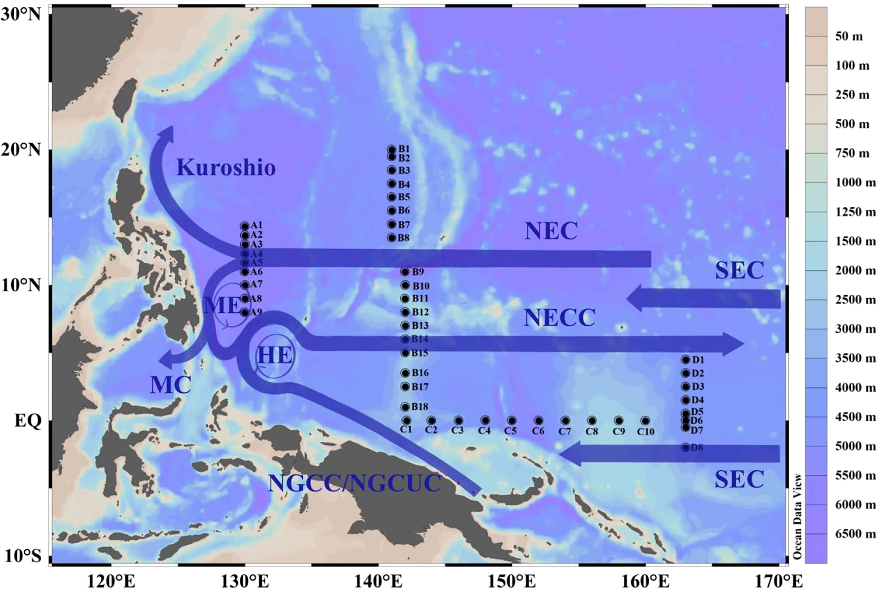
Figure 1 Station locations and currents in the study area in the WTP. NEC, North Equatorial Current, MC, Mindanao Current, NECC, North Equatorial Counter Current, SEC, South Equatorial Current, NGCC, New Guinea Coastal Current, NGCUC, New Guinea Coastal Undercurrent Current, ME, Mindanao Eddy, HE, Halmahera Eddy.

2.2 Identification of phytoplankton

CTD collected samples of the phytoplankton community structure. Samples from different water layers were placed in 1 L PE bottles, fixed with formaldehyde solution (3%), and stored in a cool place. The phytoplankton samples were shaken gently and settled in a 100 ml sedimentation column for 48 hours in the laboratory. The structure of the phytoplankton community was identified qualitatively and quantitatively under an inverted microscope (Motic AE 2000) based on Utermöhl method (Sun et al., 2002). The phytoplankton species were identified according to Jin, Isamu Y (Isamu, 1991), and Sun (Sun et al., 2002).

2.3 Analysis of the nutrient

Dissolved inorganic nitrogen (DIN), dissolved inorganic phosphorus (DIP) and dissolved silicon (DSi) were measured by colorimetric method using Technicon AA3 Auto-Analyzer (Bran Luebbe, Germany). The DIN measured included Nitrate (NO₃-N), Nitrite (NO₂-N), and Ammonium (NH₄-N). Using the cadmium-copper column reduction method to determine NO₃-N, the limit of detection (LOD) was 0.01 μmol L^-1 (Wood et al., 1967).The naphthalene ethylenediamine method was used to determine NO₂-N with a LOD of 0.01 μmol L^-1 (Wang et al., 2022). Using the sodium salicylate method to determine NH₄-N with a LOD of 0.03 µmol L^-1 (Verdouw et al., 1978). DIP was determined as PO₄-P with a LOD of 0.02 µmol L^-1 using the phosphomolybdenum blue method (Taguchi et al., 1985). DSi was determined as SiO₃-Si. The LOD was 0.02 µmol L^-1 using the silicon-molybdenum blue method (Isshiki et al., 1991).

2.4 Measurement of cell size and carbon biomass

The carbon biomass of the cells was estimated based on the cell volume with conversion factors. A fluorescence microscope (RX50) was used to measure phytoplankton-related volume parameters at a magnification of 200× (or 400×). Each phytoplankton cell was measured 25-30 times, and the volume parameters were averaged to find the cell volume (Sun et al., 1999). Calculate the cell volume regarding Sun’s model and formula (Sun and Liu, 2003). Biomass calculation was based on Eppley (Eppley et al., 1970):

$$\text{Diatoms}:lo{g}_{10}C=0.76lo{g}_{10}V-0.352$$

$$\text{Other microalgae}:lo{g}_{10}C=0.94lo{g}_{10}V-0.60$$

represents the single-cell volume (μm³); $C$represents the single-cell carbon biomass (pg).

The phytoplankton importance was calculated using the method of Sun (Sun, 2004):

$$K=\frac{B_i}{B}·f_i$$

where $K$ is the importance of keystone species in the survey; $B_i$ is the total carbon biomass of species $i$ (μg L^-1); $B$ is the total carbon biomass of all phytoplankton (nanophytoplankton and microphytoplankton) in one survey (μg L^-1); $f_i$ is the frequency of occurrence of species $i$ in the survey.

In this study, phytoplankton carbon biomass in the water column calculated using trapezoidal integration (Uitz et al., 2006):

$$C=\left[\sum _{i=1}^{n-1}\frac{C_{i+1}+C_i}{2}·(D_{i+1}-D_i)\right]/(D_{max}-D_{min})$$

where $C$ is the average value of phytoplankton carbon biomass in water column (mg m^-3); $n$ is the total number of layers sampled; $C_i$ is the carbon biomass of layer $i$ (mg m^-3); $D_i$ is the sampling depth of layer $i$ (m); $D_{max}$ represents the maximum sampling depth and $D_{min}$ represents the minimum sampling depth (m).

2.5 Data analysis

Calculation of the dominance of phytoplankton:

$$Y=(\frac{n_i}{N})\times f_i$$

$N$ is the total number of individuals; $n_i$ is the number of individuals of species i; $f_i$ is the frequency of occurrence of species i.

The Shannon index was calculated using the “Vegan” package (Oksanen et al., 2022) in R version 4.2.1, and significance was tested using the Wilcoxon rank-sum test. To account for the heterogeneous cell size distribution in the studied sea area, quantile regression was used to analyze cell size trends, as it provides a clearer understanding of cell volume. Quantile regressions of cell size were calculated using the “quantreg” package (Maniaci et al., 2022) in R version 4.2.1, and significance was determined using the P-test. Pearson’s correlation coefficient was used to assess the relationship between phytoplankton abundance, diversity of phytoplankton and environmental factors. Canonical Correspondence Analysis (CCA) was performed using Canoco 5.0 on the cell abundance of species and environmental factors, with both data sets being log10(x+1) transformed. The species data consisted of the abundance of the top 60 dominant species. Hierarchical Clustering was used for cluster analysis of phytoplankton, and the dissimilarity between different groups of phytoplankton was calculated using Primer 6 (6.1.12.0).

3 Results

3.1 Hydrology and nutrients analyses

In 2019, the surface temperature distribution in the western Tropical Pacific Ocean (WTP) was characterized by high values, with a mean surface temperature of about 28°C, which is a typical feature of the western Pacific warm pool (Figures 2A-D). The water temperature decreased unevenly with increasing depth, and a sharp thermocline was observed at around 100 m at all sections. Salinity also increased unevenly with depth, due to the presence of North Pacific Tropical Water and South Pacific Tropical Water at the thermocline (Figures 2E–H). In section B (2°-15°N), both isothermals and isohalines were elevated. The subsurface water temperature and salinity were higher in sections C and D near the equator, owing to the warm pool and saline South Pacific Tropical Water (Figures 2C, D, G, H). Surface nutrients were deficient and only gradually increased at depths of 100 m (Figure 3). Similar to the vertical distribution of temperature and salinity, nutrients had a bump in the 2°-15°N section of section B (Figures 3B, F, J)

FIGURE 2

Figure 2 Vertical distribution of temperature (A–D) and salinity (E–H) in the WTP in 2019.

FIGURE 3

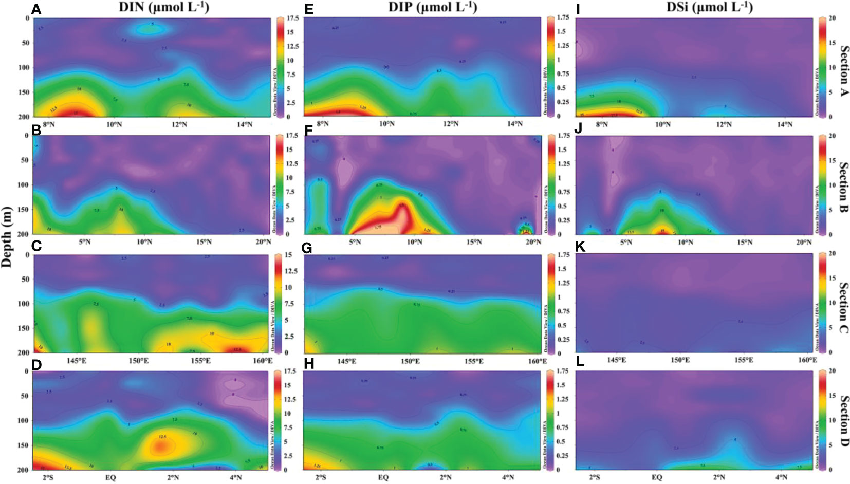
Figure 3 Vertical distribution of nutrients (μmol L^-1) in the WTP in 2019. (A-D) vertical distribution of DIN; (E-H) vertical distribution of DIP; (I-L) vertical distribution of DSi.

3.2 Species composition and community structure of phytoplankton

This investigation identified a total of 260 species from 4 phyla: Bacillariophyta, Dinophyta, Cyanophyta, and Chrysophyta, across 64 genera (Table S1). Diatoms were represented by 33 genera and 73 species, dinoflagellates by 28 genera and 181 species, cyanobacteria by 2 genera and 4 species, and chrysophyceae by 1 genus and 2 species. Dinoflagellates had the largest number of species, accounting for 69.92% of the total species with a cell abundance of 9698 cells L^-1. Diatoms made up 28.08% of the species with a cell abundance of 9026 cells L^-1. Cyanobacteria had the highest cell abundance of 121,398 cells L^-1, but their species accounted for only 1.54% of the total. The smallest proportion of both species and cell abundance was from chrysophyceae, at 0.77% and 896 cells L^-1, respectively. The top ten dominant species identified in the investigation included four dinoflagellates, three cyanobacteria, and three diatoms (Table 1).

TABLE 1

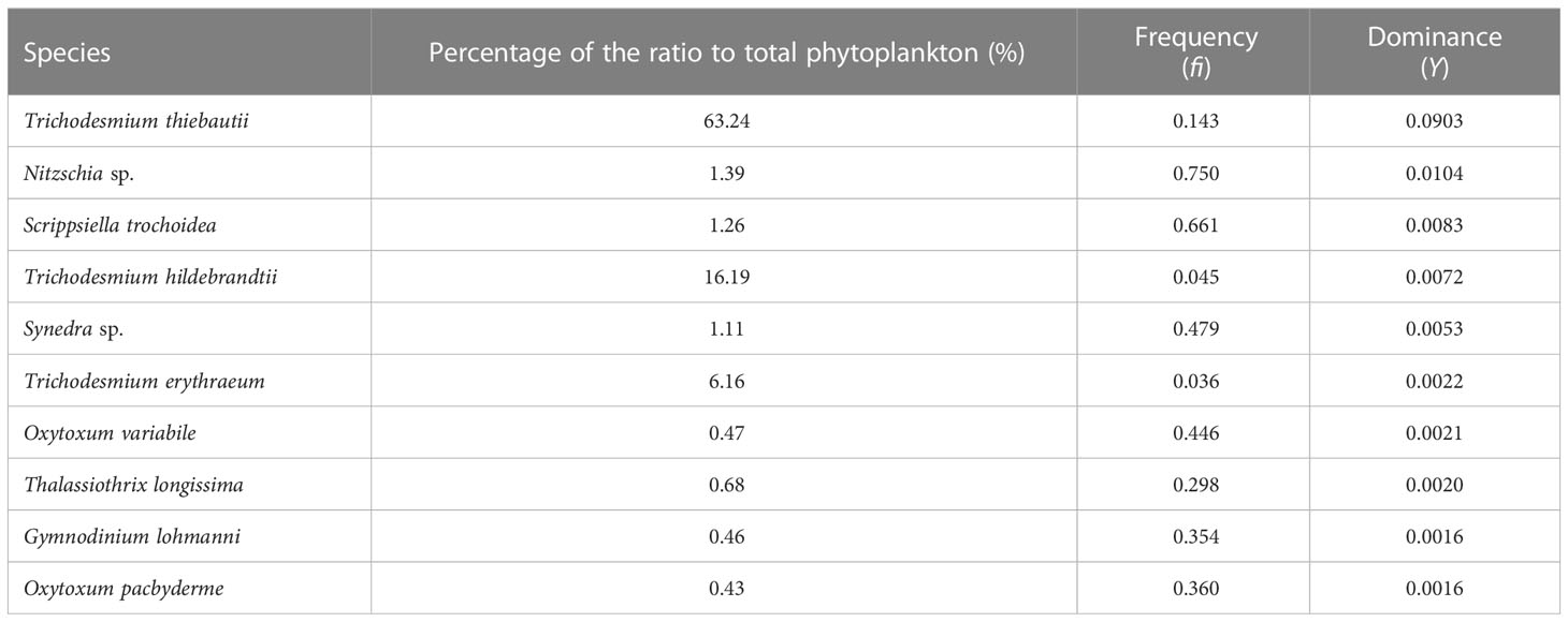
Table 1 Dominant phytoplankton species in the WTP.

Overall, the distribution of phytoplankton varied significantly among the four sections (Figure 4A). Dinoflagellates were found to be evenly distributed across all four sections. Section B had the highest proportion of cyanobacteria, while the proportion of diatoms sharply increased in sections B9-B15. Sections C and D had a similar phytoplankton composition, with higher levels of diatoms near land in section C. The dominant species of phytoplankton also differed across the sections (Figure 4B). Trichodesmium thiebautii was the dominant species in stations A1, A2, A8, and A9, while Scrippsiella trochoidea, Nitzschia sp., and Thalassiothrix longissima were the dominant species in other stations. Section B was mainly dominated by Trichodesmium thiebautii, Trichodesmium hildebrandtii, and Trichodesmium erythraeum, except for stations B9-B12 and B14, which had high levels of diatoms such as Nitzschia sp. and Synedra sp. Sections C and D had a similar phytoplankton composition, with dominant species including Synedra sp., Scrippsiella trochoidea, Nitzschia sp., Thalassiothrix longissima, Dictyocha fibula and Coscinodiscus granii.

FIGURE 4

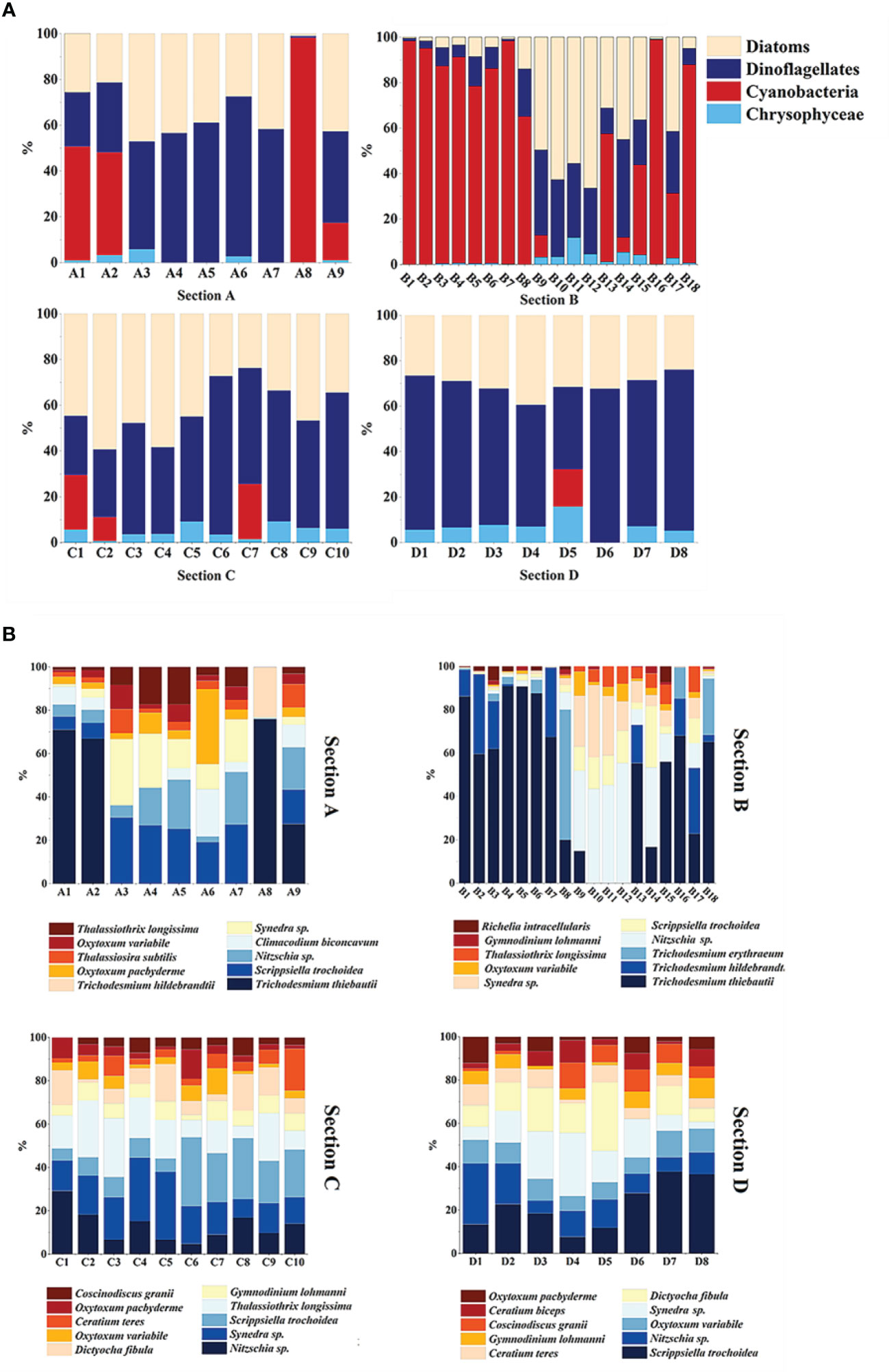
Figure 4 Composition of phytoplankton (A) and dominant species (B) in four sections in the WTP.

For the diversity of phytoplankton, the Shannon diversity index of sites B1-B8 is lower, while sections C and D near the equator have higher diversity (Figure 5). Therefore, the difference in planktonic plant diversity between section B and sections C and D is very significant, while the difference relative to section A is relatively small.

FIGURE 5

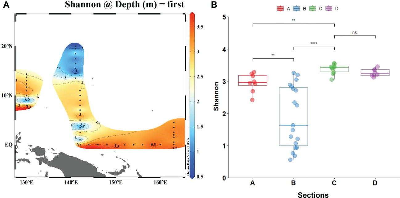
Figure 5 Comparison of Shannon diversity index between all stations (A) and four sections (B). (The significance results of section D between sections A and B were the same as those of section C). “*” represents significance, *: p < 0.05, **: p < 0.005, ***: p < 0.001. “ns” means no significance.

3.3 Cell size of phytoplankton

When cell abundance was regressed against equivalent sphere diameter (ESD) using all data, a high degree of significance was found (p-value< 0.01), with 38.1% of the change in abundance being explained by ESD. The slope of the fitted straight line of cell abundance versus ESD increased with increasing cell volume, indicating that the decrease in cell abundance rate is faster when the cells are larger (Figure 6A). However, the slope hardly changes when the quantile is 0.01-0.3 (Figure 6C), suggesting that cell abundance is high and does not vary much in this ESD range of approximately 2 to 12 μm. At a quantile of approximately 0.3, the slope decreases, indicating that the abundance of cells with ESD greater than 12 μm begins to decrease. At quantile 0.8, the slope decreases again, and the ESD is about 25 μm, indicating that the abundance of cells with ESD greater than 25 μm is small, and the abundance of cells becomes smaller as the cell volume increases.

FIGURE 6

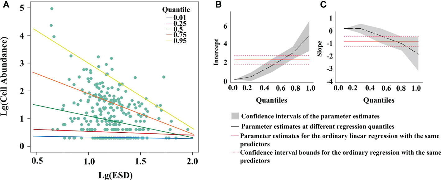
Figure 6 Quantile regression analysis of equivalent sphere diameter (ESD) versus cell abundance in the WTP. Least squares fit to log 10 transformed data. (A) Results of fitting ESD to cell abundance at different percentile; (B) intercepts of different interquartile fits; (C) slopes of different interquartile fits.

3.4 Distribution of phytoplankton cell abundance and carbon biomass

Along sections A and B, cell abundance was dominated by cyanobacteria, which were present only in the surface layer (Figures 7C, O). In section A, cell abundance distribution was similar for diatoms and dinoflagellates, but diatoms distributed in deeper layers (Figures 7A, B). The cell abundance of chrysophyceae was small and mainly distributed in the subsurface layer (Figure 7D). Compared to microphytoplankton, nanophytoplankton had a giant cell abundance and was mainly distributed in the upper layers, while microphytoplankton was mainly distributed in the lower layers (Figures 7E, F). Notably, cyanobacteria were more widespread in section B (Figure 7O) and phytoplankton were distributed in deeper layers compared to section A (Figures 7Q, R).

FIGURE 7

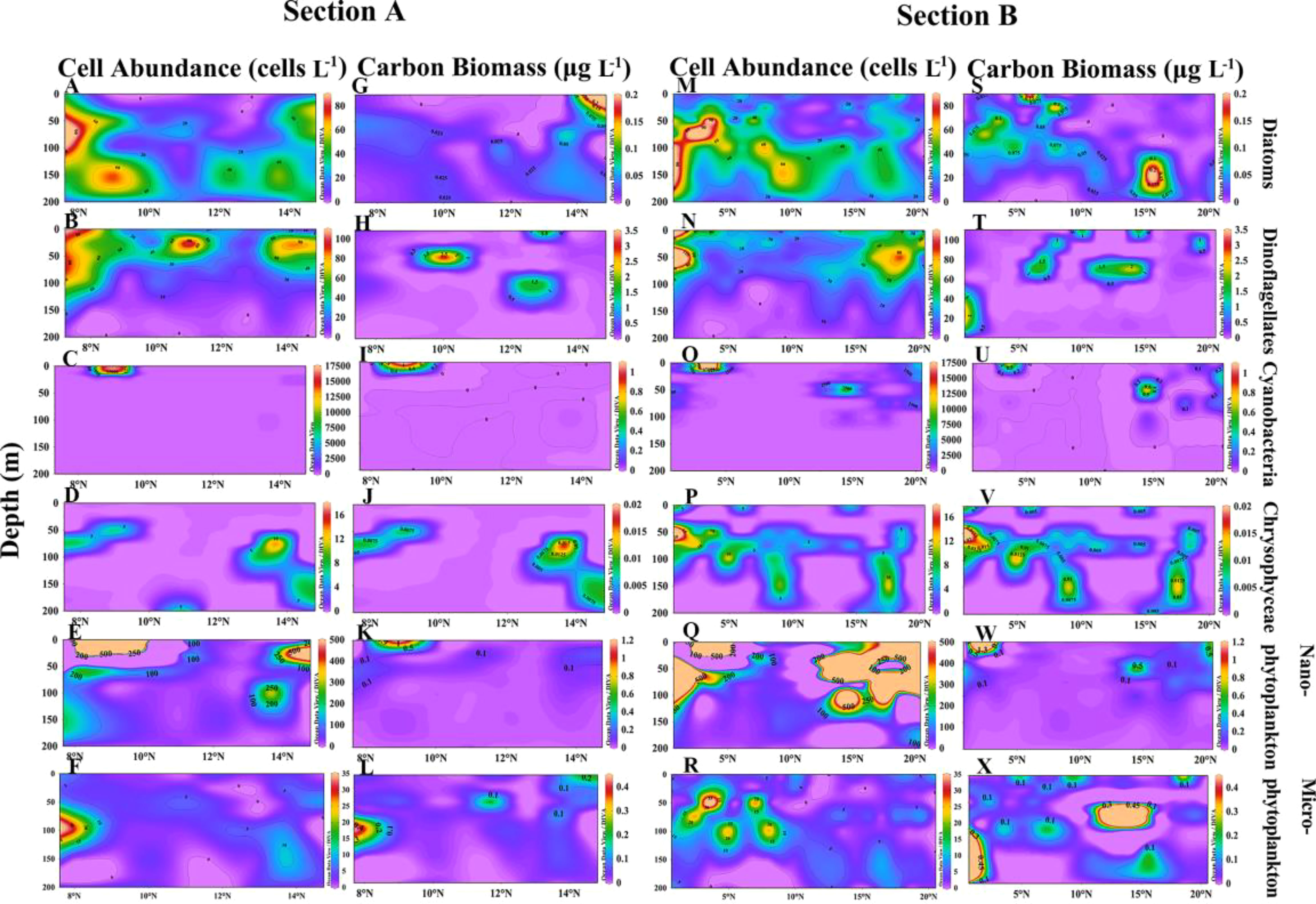
Figure 7 Vertical distribution of cell abundance and carbon biomass of phytoplankton in sections A and B. Cell abundance and carbon biomass of diatoms (A, G), dinoflagellates (B, H), cyanobacteria (C, I), chrysophyceae (D, J), nanophytoplankton (E, K) and microphytoplankton (F, L) in section A; Cell abundance and carbon biomass of diatoms (M, S), dinoflagellates (N, T), cyanobacteria (O, U), chrysophyceae (P, V), nanophytoplankton (Q, W) and microphytoplankton (R, X) in section B.

The cell abundance and carbon biomass of sections C and D are shown in Figure 8. In sections C and D, the phytoplankton abundance was dominated by dinoflagellates and diatoms, with little presence of cyanobacteria (Figures 8A–C, M–O). Dinoflagellates were primarily concentrated in the surface layer (Figure 8B), while the abundance of diatoms and chrysophyceae increased in section C, especially near land (Figures 8A, D). The cell abundance of microphytoplankton was greatest in section C, mainly distributed around 75m, and the cell abundance in section D was the smallest among all sections (Figures 8Q, R). The cell abundance of diatoms in section D decreased and was almost exclusively distributed in the subsurface layer (Figure 8A).

FIGURE 8

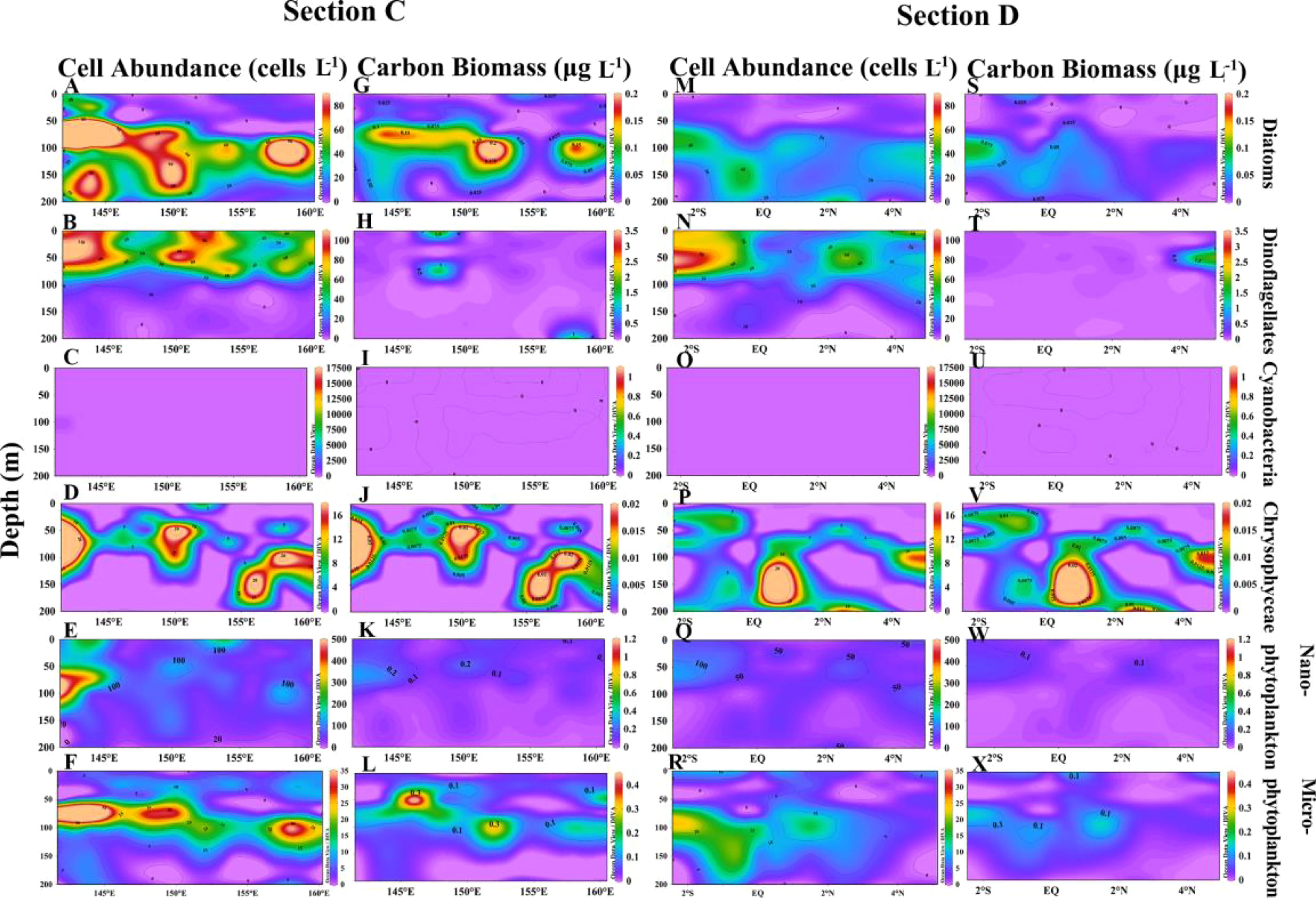
Figure 8 Vertical distribution of cell abundance and carbon biomass of phytoplankton in sections C and D. Cell abundance and carbon biomass of diatoms (A, G), dinoflagellates (B, H), cyanobacteria (C, I), chrysophyceae (D, J), nanophytoplankton (E, K) and microphytoplankton (F, L) in section C; Cell abundance and carbon biomass of diatoms (M, S), dinoflagellates (N, T), cyanobacteria (O, U), chrysophyceae (P, V), nanophytoplankton (Q, W) and microphytoplankton (R, X) in section D.

The carbon biomass in the survey area ranged from 6.597 mg m^-3 to 155.627 mg m^-3, with a mean value of 25.969 ± 24.752 mg m^-3 (Table S1). The carbon biomass of different species and cell sizes of phytoplankton were examined separately (Figures 9A, B). In terms of phytoplankton species, the carbon biomass of dinoflagellates, diatoms, cyanobacteria, and chrysophyceae was 674.266 mg m^-3, 338.329 mg m^-3, 125.266 mg m^-3, and 30.758 mg m^-3, respectively, accounting for 57.698%, 28.951%, 10.719%, and 2.632%, respectively (Figure 9A). Dinoflagellates contributed more than 50% of the carbon in each section. The carbon contribution of diatoms increased in sections C and D, with an abrupt increase at stations B9 to B17. The carbon contributed by cyanobacteria was mainly concentrated in stations A8, B1-B7, and B16. In terms of phytoplankton size, the total carbon biomass of nanophytoplankton and microphytoplankton was 376.324 mg m^-3 and 792.295 mg m^-3, respectively, accounting for 32.202% and 67.798% of the total carbon biomass (Figure 9B). The carbon contribution of microphytoplankton exceeded 60% in each section.

FIGURE 9

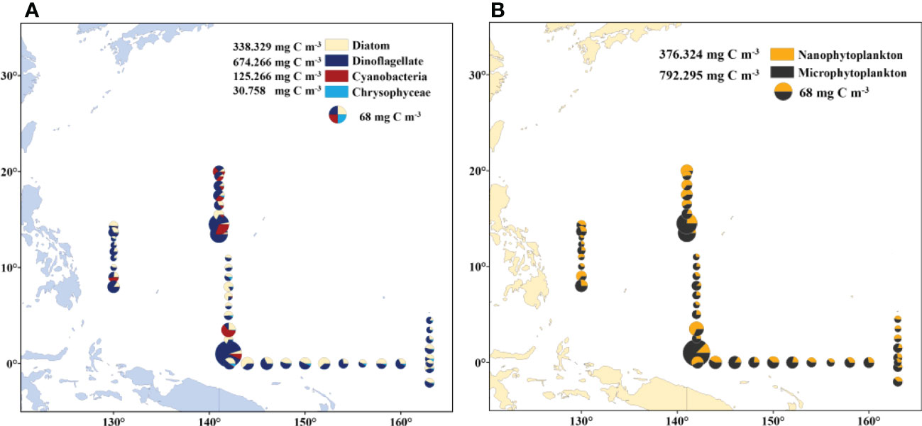
Figure 9 Spatial distribution of carbon biomass of phytoplankton. (A) Carbon biomass distribution of diatoms, dinoflagellates, cyanobacteria and chrysophyceae; (B) carbon biomass of nanophytoplankton and microphytoplankton.

Analysis of the vertical distribution of carbon biomass revealed that diatoms contributed the most to the carbon biomass in sections B and C, and were primarily distributed in the subsurface layer (Figures 7S, 8G). In contrast, dinoflagellates and cyanobacteria showed higher carbon biomass in the upper layer (Figures 7H, T, I, U, 8H, T, I, U). Nanophytoplankton contributed more carbon biomass in sections A and B, and were primarily found in the surface layer (Figures 7K, W). The carbon biomass of microphytoplankton was highest in section B, and mainly concentrated in the subsurface layer (Figures 7X).

3.5 Keystone species for carbon biomass

To better understand the role of low abundance and high volume cells in the ecosystem, this study utilized a combination of phytoplankton carbon biomass and dominance calculations to identify key species in the WTP phytoplankton community (Table 2). The importance of each species to carbon biomass was used to determine the keystone species, with dinoflagellates (3 species) and diatoms (2 species) being the primary contributors, followed by cyanobacteria (1 species). Scrippsiella trochoidea was frequently observed and had the highest importance among the identified keystone species, while Coscinodiscus granii had the highest single-cell carbon biomass (Table 2). Trichodesmium thiebautii was also considered a keystone species due to its high abundance despite its minimal single-cell carbon amount.

TABLE 2

Table 2 Keystone species and their carbon biomass in the WTP.

The carbon biomass of dinoflagellates and cyanobacteria peaked at depths of 5-50 m, with Trichodesmium thiebauti and Ceratium pulchellum having the highest mean carbon biomass at 5 m, at 0.430 μg L^-1 and 0.583 μg L^-1, respectively (Figures S2D, F). The peak carbon biomass of Gymnodinium lohmanni was observed at 50 m, with 0.395 μg L^-1 (Figure S2C). In contrast, diatoms had a deeper distribution, with the peak carbon biomass of Coscinodiscus granii at 100 m (0.280 μg L^-1) (Figure S2B), and Synedra sp. at 150 m (0.359 μg L^-1) (Figure S2E).

3.6 Community structure and hydrological characteristics of four groups of phytoplankton

Cluster analysis was employed to classify phytoplankton into four groups. The results showed that group 1 and group 2 were highly similar, while group 3 and group 4 were also highly similar (Figure 10). Compared to group 2, group 1 had a higher diatom abundance, with Nitzschia sp. and Thalassiothrix longissima having the highest abundance among the four groups (Table 3). In group 2, the abundance of Trichodesmium thiebautii was the highest among the four groups, but Trichodesmium hildebrandtii and Trichodesmium erythraeum were not observed. Group 3 exhibited distinct characteristics of low temperature and low salinity, with the highest diatom abundance. Synedra sp. and Thalassiothrix longissima also had higher abundance in group 3.

FIGURE 10

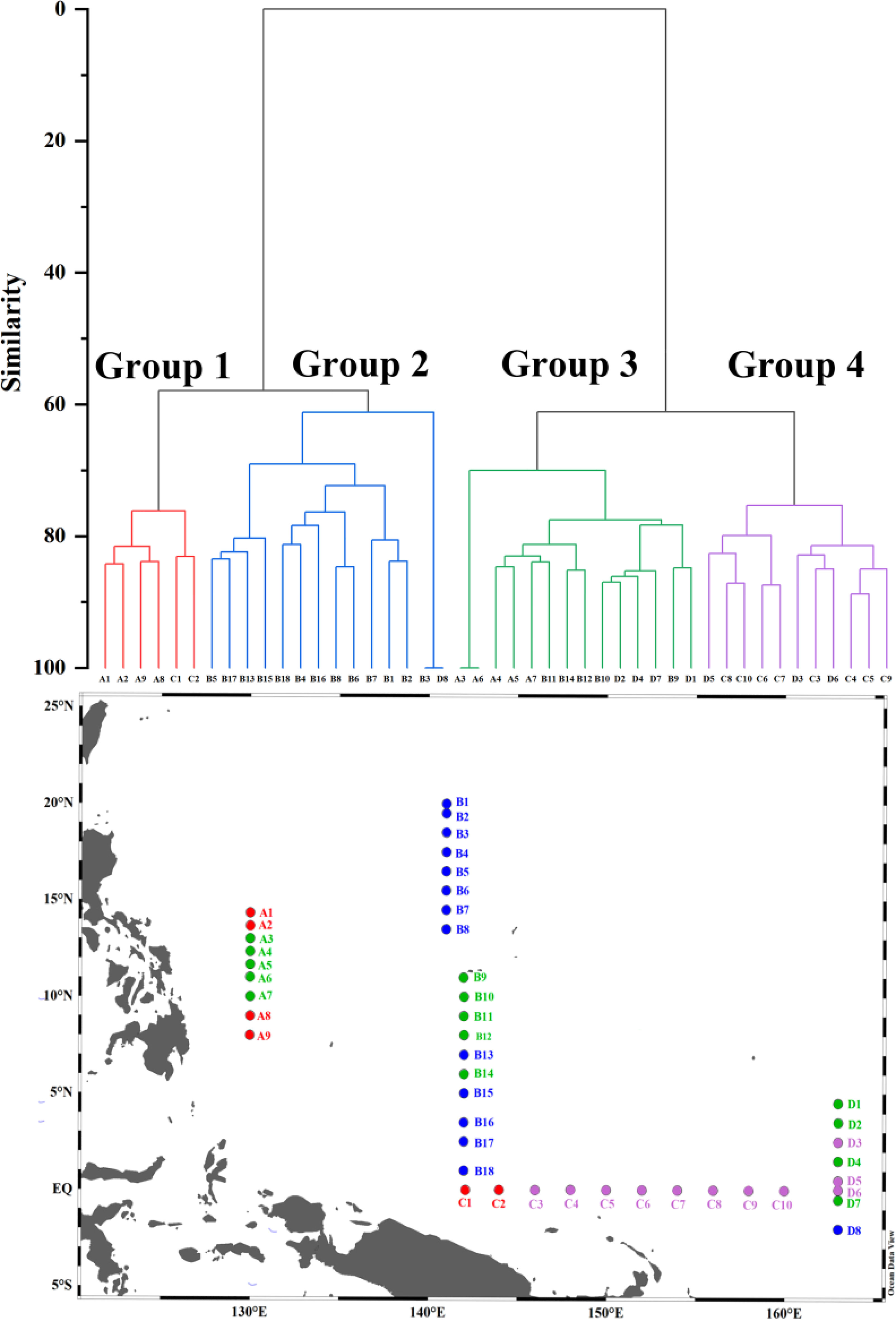
Figure 10 Results and location of cluster analysis of phytoplankton composition in the WTP.

TABLE 3

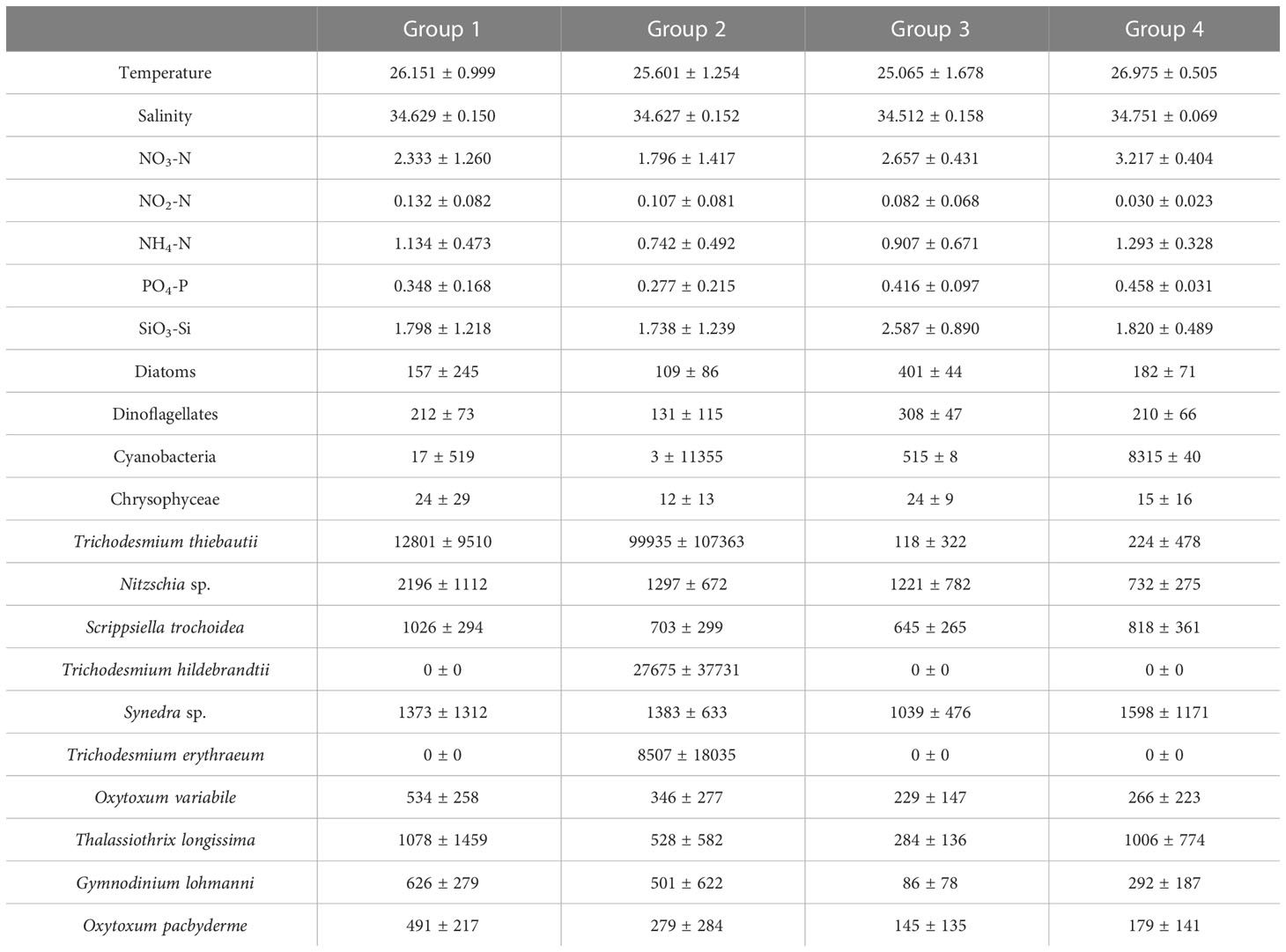
Table 3 Mean values of temperature (℃), salinity, nutrients (μmol L^-1) and species cell abundance (cells L^-1) of four groups of phytoplankton obtained by clustering analysis.

3.7 Environmental effects on phytoplankton community, cell size and carbon biomass

The Pearson correlation reflects the relationship between phytoplankton and environmental factors (Figure S3). Cyanobacteria were highly significantly and positively correlated with temperature, suggesting that temperature may affect their distribution. Dinoflagellate abundance was highly significantly and positively correlated with temperature and negatively correlated with nutrition, reflecting that the growth of dinoflagellates is susceptible to temperature. At the same time, dinoflagellates may can survive better under nutrient-deficient conditions. Diatom abundance was positively correlated with DIN and DIP, indicating that nutrients can influence the distribution of diatoms. Microphytoplankton was extremely significantly and positively correlated with diatoms reflecting that it is mainly composed of diatoms. Several diatom species, such as Thalassiothrix longissimi and Synedra sp., were positively correlated with nitrate and negatively correlated with temperature (Figure 11). In contrast, the majority of cyanobacteria and dinoflagellate species showed a negative correlation with nitrate and a positive correlation with temperature, such as Trichodesmium thiebautii and Scrippsiella trochoidea.

FIGURE 11

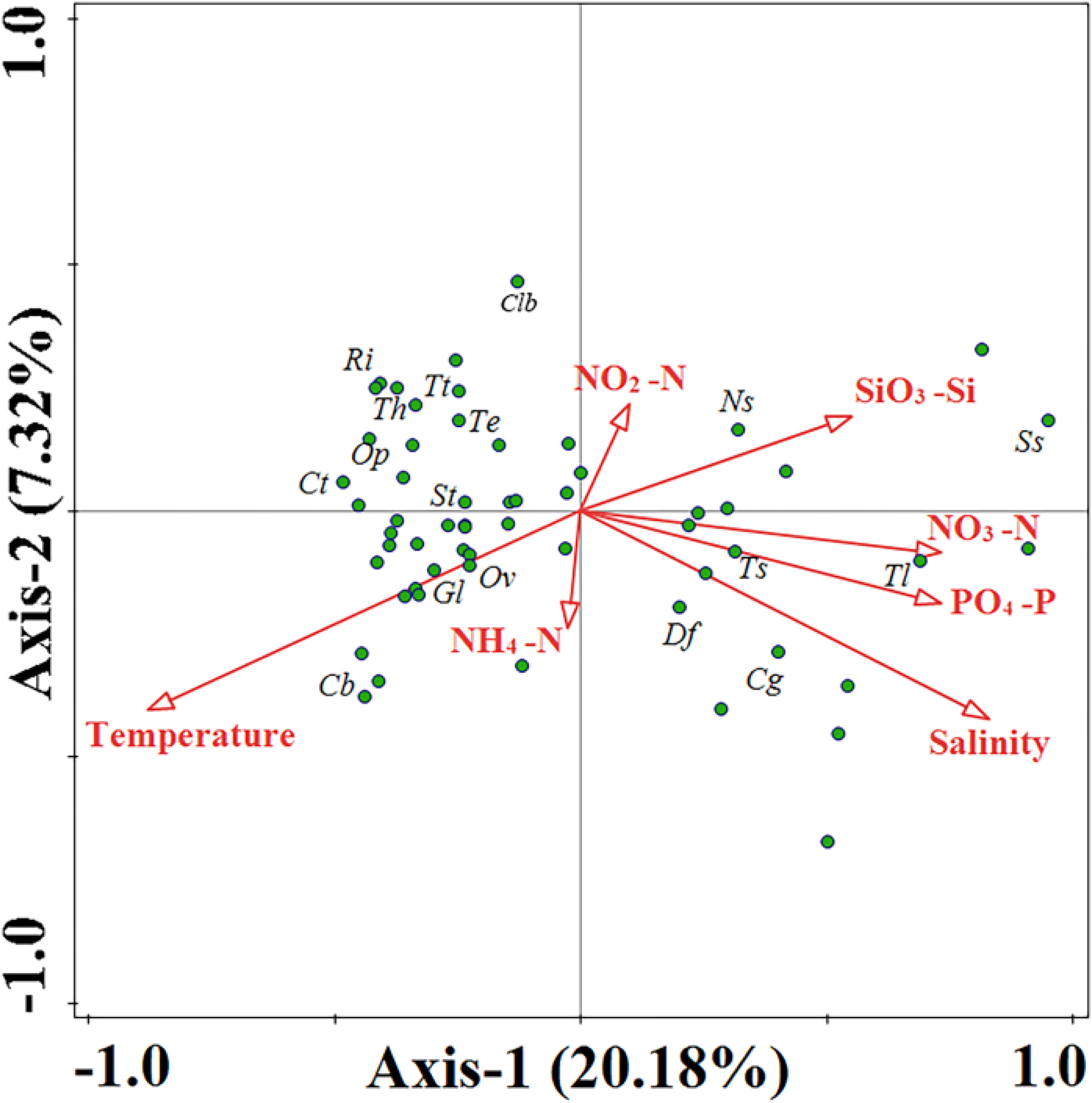
Figure 11 Canonical Correspondence Analysis (CCA) of phytoplankton species and environmental factors in the WTP. Clb, Climacodium biconcavum; Ri, Richelia intracellularis; Tt, Trichodesmium thiebautii; Th, Trichodesmium hildebrandtii; Te, Trichodesmium erythraeum; Ct, Ceratium teres; St, Scrippsiella trochoidea; Gl, Gymnodinium lohmanni; Ov, Oxytoxum variabile; Op, Oxytoxum pacbyderme; Cb, Ceratium biceps; Ns., Nitzschia sp.; Ss., Synedra sp.; Tl, Thalassiothrix longissimi; Ts, Thalassiosira subtilis; Df, Dictyocha fibula; Cg, Coscinodiscus granii.

4 Discussion

4.1 Classification of phytoplankton and their corresponding hydrological environments

We used cluster analysis to divide phytoplankton into four groups, and the differences in phytoplankton composition between stations reflected changes in ocean currents, which profoundly affected the diversity and distribution of phytoplankton. Although the changes in phytoplankton composition cannot be strictly distinguished by ocean currents, the variation in phytoplankton at different sections still showed certain patterns. For instance, in section A, the phytoplankton composition underwent a transition from Group 1 to Group 3 and then back to Group 1, respectively, which confirms that this section was impacted by the influence of distinct water masses. Kuroshio, known for its high temperature and low nutrient levels, provides suitable conditions for the growth of cyanobacteria, resulting in an increase in cyanobacteria abundance at stations A1 and A2 (Figures 4A, S3). Although station A9 is also classified under Group 1, it may be affected by the Mindanao Eddy, which brings up nutrient-rich cold water to the surface within the eddy. This causes the thermocline depth to become shallower, promoting the growth of diatoms, according to Zhang’s study (Zhang Q. et al., 2012). Unlike Group 1, Group 3 had the lowest temperature and salinity and higher nitrate concentration (Table 3). This may be due to the current-seamount interaction generated by the North Equatorial Current encountering seamounts at stations B9-B12 (Figures 1–3), consistent with the research by Ma (Ma et al., 2019). This effect creates a unique phytoplankton community structure in Group 3, which is dominated by diatoms that prefer low temperature and high nutrients (Figures 4B, 11). Except for the stations affected by current-seamount interaction, the phytoplankton in section B was dominated by cyanobacteria, with low species diversity, possibly due to minimal ocean current influence and distance from the land (Figure 1). In contrast to section B, the species diversity in sections C and D was high (Figure 5). On the one hand, the thermocline in the eastern equatorial Pacific is much lower than that in the western Tropical Pacific Ocean, and nutrient-rich seawater is transported by the South Equatorial Current to the Gulf of Papua, and nutrient levels are increasing due to the influence of the New Guinea continent (Gordon and Fine, 1996; Mackey et al., 2002). On the other hand, the New Guinea coastal upwelling, which flows southeast to northwest year-round, also carries high salinity and nutrient-rich South Pacific water northward along the coast (Christian et al., 2004). Therefore, the waters outside the New Guinea Islands have higher species diversity and diatom biomass (Figure 5, 9A), consistent with the research by Dong (Dong et al., 2012).

4.2 Environmental preferences of dominant species

Different dominant species exhibit specific environmental preferences and can significantly influence the characteristics of entire ecological communities. Our study employs both cluster analysis and CCA analysis to identify two distinct types of phytoplankton: the high-temperature low-nitrate type, represented by Trichodesmium and Scrippsiella trochoidea, and the low-temperature high-nitrate type, represented by Thalassiothrix longissima and Synedra sp. (Figures 10, 11). Trichodesmium, a crucial nitrogen-fixing alga in the ocean, contributes substantially to primary production and biomass in our study area. However, factors such as wind, phosphorus, and unique metal characteristics can significantly impact the abundance of Trichodesmium (Chang et al., 2000; Nuester et al., 2012). Our survey has indicated that Trichodesmium erythraeum and Trichodesmium hildebrandtii solely appeared in Group 2, suggesting their affinity for living in undisturbed oligotrophic water bodies. Chen’s research also supports our findings, demonstrating that Trichodesmium thiebautii primarily dominates areas outside the New Guinea Islands with large ocean currents. Conversely, Trichodesmium erythraeum and Trichodesmium hildebrandtii have a greater abundance in sections unaffected by ocean currents (5°-35°N, 145°E). Scrippsiella trochoidea, a dominant and key species in the western Tropical Pacific Ocean, exhibits widespread distribution and high abundance across four sections, ranging from northern to tropical waters. This species has been reported to bloom in various regions, such as Japan, the Mediterranean, and the US coast (Montresor et al., 1998; Zinssmeister et al., 2011; Morozova et al., 2016). Our survey has also revealed that Scrippsiella trochoidea can maintain high density even in low-nutrient conditions, corroborating existing literature (Yin et al., 2008).

The dominant diatom species identified in this survey mostly belong to nanophytoplankton. The small cell size of these diatoms enables them to remain suspended and to rapidly absorb nutrients. Some diatom species have become elongated or flattened to increase their surface area-to-volume ratio for better nutrient absorption (Reynolds, 2006), such as Thalassiothrix longissima and Synedra sp. (Figure S1). Ceratium biceps is an important species that distinguishes Group 3 from Group 4 (Table S4). It prefers high-salinity conditions of Group 4 (Table 3), which is consistent with the results of CCA analysis (Figure 11). In the continental shelf area close to land, the abundance of Ceratium biceps is higher, which is consistent with the findings (Hallegraeff and Jeffrey, 1984).

5 Conclusion

We investigated the community structure, cell size, and carbon biomass of phytoplankton in the western Tropical Pacific Ocean in 2019. The phytoplankton community was mainly composed of dinoflagellates (181 species), diatoms (73 species), cyanobacteria (4 species), and chrysophyceae (2 species), with most species having equivalent spherical diameters of 2-12 µm and dominated by nanophytoplankton. Despite their lower abundance, microphytoplankton contributed 792.295 mg m^-3 of carbon, while nanophytoplankton contributed 376.324 mg m^-3. In this study, we found that the composition and distribution of phytoplankton were closely related to ocean currents. For example, the abundance of diatoms increased under the influence of the South Equatorial Current and the coastal currents of the New Guinea Coastal Undercurrent Current, while the abundance of Trichodesmium was very high in areas with little disturbance from ocean currents. Overall, this survey provided valuable insights into the distribution and composition of phytoplankton in the western tropical Pacific Ocean. It highlighted the relationship between species distribution and ocean currents and provided basic information on cell size and carbon biomass in the region.

Data availability statement

The original contributions presented in the study are included in the article/Supplementary Material. Further inquiries can be directed to the corresponding author.

Author contributions

JS: Conceptualization, Methodology, Project administration, Resources, Supervision, Visualization, Review & editing. WY: Sample measurement, Data analysis, Writing the manuscript. ZC: Sample identification, Data analysis. FW and GZ: Sample collection, Environmental factor determination. LZ: CTD data interpretation and review. All authors contributed to the article and approved the submitted version.

Funding

This research was supported by the National Natural Science Foundation of China (41876134), and the Changjiang Scholar Program of the Chinese Ministry of Education (T2014253) through grants to Jun Sun. The research was also partially supported by the State Key Laboratory of Biogeology and Environmental Geology, China University of Geosciences (GKZ22Y656).

Acknowledgments

CTD data and water samples were collected on board of R/V KeXue implementing open research cruises NORC2019-09 and NORC2021-09 supported by NSFC Shiptime Sharing Projects (Nos. 41849909 and 42049909) and Laoshan Science and Technology Innovation project (No. LSKJ202201700).

Conflict of interest

The authors declare that the research was conducted in the absence of any commercial or financial relationships that could be construed as a potential conflict of interest.

Publisher’s note

All claims expressed in this article are solely those of the authors and do not necessarily represent those of their affiliated organizations, or those of the publisher, the editors and the reviewers. Any product that may be evaluated in this article, or claim that may be made by its manufacturer, is not guaranteed or endorsed by the publisher.

Supplementary material

The Supplementary Material for this article can be found online at: https://www.frontiersin.org/articles/10.3389/fmars.2023.1147271/full#supplementary-material

References

Chang J., Chiang K.-P., Gong G.-C. (2000). Seasonal variation and cross-shelf distribution of the nitrogen-fixing cyanobacterium, trichodesmium, in southern East China Sea. Cont Shelf Res. 20 (4), 479–492. doi: 10.1016/S0278-4343(99)00082-5

CrossRef Full Text | Google Scholar

Charalampous E., Matthiessen B., Sommer U. (2021). Grazing induced shifts in phytoplankton cell size explain the community response to nutrient supply. Microorganisms 9 (12), 2440. doi: 10.3390/microorganisms9122440

PubMed Abstract | CrossRef Full Text | Google Scholar

Chen Z., Sun J., Gu T., Zhang G., Wei Y. (2021). Nutrient ratios driven by vertical stratification regulate phytoplankton community structure in the oligotrophic western pacific ocean. Ocean Sci. 17 (6), 1775–1789. doi: 10.5194/os-17-1775-2021

CrossRef Full Text | Google Scholar

Chen Z., Sun J., Zhang G. (2018). Netz-phytoplankton community structure of the tropical Western pacific ocean in summer 2016. Mar. Sci. 42 (7), 114–130. doi: 10.11759//hykx20180331002

CrossRef Full Text | Google Scholar

Chen Y., Sun X., Zhu M., Zheng S., Yuan Y., Denis M. (2017). Spatial variability of phytoplankton in the pacific western boundary currents during summer 2014. Mar. Freshw. Res. 68 (10), 1887–1900. doi: 10.1071/MF16297

CrossRef Full Text | Google Scholar

Christian J., Murtugudde R., Ballabrera J., McClain C. (2004). A ribbon of dark water: phytoplankton blooms in the meanders of the pacific north equatorial countercurrent. Deep Sea Res. Part II: Topical Stud. Oceanography 51, 209–228. doi: 10.1016/j.dsr2.2003.06.002

CrossRef Full Text | Google Scholar

Dong L., Li L., Wang H., He J., Wei Y. (2012). PHYTOPLANKTON DISTRIBUTION IN SURFACE WATER OF WESTERN PACIFIC DURING WINTER 2008: a STUDY OF MOLECULAR ORGANIC GEOCHEMISTRY. Mar. Geology Quaternary Geology 32, 51–60. doi: 10.3724/SP.J.1140.2012.01051

CrossRef Full Text | Google Scholar

Eppley R. W., Reid F. M. H., Strickland J. D. H. (1970). Estimates of phytoplankton crop size, growth rate, and primary production. Bull. Scripps Inst Oceanogr 17, 33–42.

Google Scholar

Finkel Z. V. (2001). Light absorption and size scaling of light-limited metabolism in marine diatoms. Limnol Oceanogr 46 (1), 86–94. doi: 10.4319/lo.2001.46.1.10086

CrossRef Full Text | Google Scholar

Finkel Z. V., Beardall J., Flynn K. J., Quigg A., Rees T. A. V., Raven J. A. (2010). Phytoplankton in a changing world: cell size and elemental stoichiometry. J. Plankton Res. 32, 119–137. doi: 10.1093/PLANKT/FBP098

CrossRef Full Text | Google Scholar

Finkel Z. V., Irwin A., Schofield O. (2004). Resource limitation alters the 3/4 size scaling of metabolic rates in phytoplankton. Mar. Ecol-Prog Ser. 273, 269–279. doi: 10.3354/meps273269

CrossRef Full Text | Google Scholar

Gordon A. L., Fine R. A. (1996). Pathways of water between the pacific and Indian oceans in the Indonesian seas. Nature 379 (6561), 146–149. doi: 10.1038/379146a0

CrossRef Full Text | Google Scholar

Gosselain V., Hamilton P., Descy J.-P. (2000). Estimating phytoplankton carbon from microscopic counts: an application for riverine systems. Hydrobiologia 438, 75–90. doi: 10.1023/A:1004161928957

CrossRef Full Text | Google Scholar

Hallegraeff G., Jeffrey S. W. (1984). Tropical phytoplankton species and pigments of continental shelf waters of north and north-West Australia. Mar. Ecol-Prog Ser. 20, 59–74. doi: 10.3354/meps020059

CrossRef Full Text | Google Scholar

Hillebrand H., Dürselen C.-D., Kirschtel D., Pollingher U., Zohary T. (1999). Biovolume calculation for pelagic and benthic microalgae. J. Phycol 35, 403–424. doi: 10.1046/j.1529-8817.1999.3520403.x

CrossRef Full Text | Google Scholar

Hu D., Wang F., Sprintall J., Wu L., Riser S., Cravatte S., et al. (2020). Review on observational studies of western tropical pacific ocean circulation and climate. J. Oceanology Limnology 38 (4), 906–929. doi: 10.1007/s00343-020-0240-1

CrossRef Full Text | Google Scholar

Irion S., Christaki U., Berthelot H., L’Helguen S., Jardillier L. (2021). Small phytoplankton contribute greatly to CO2-fixation after the diatom bloom in the southern ocean. ISME J. 15 (9), 2509–2522. doi: 10.1038/s41396-021-00915-z

PubMed Abstract | CrossRef Full Text | Google Scholar

Isamu Y. (1991). Illustrations of the marine plankton of Japan (Hoikusha Press: Tokyo, Japan).

Google Scholar

Isshiki K., Sohrin Y., Nakayama E. (1991). Form of dissolved silicon in seawater. Mar. Chem. 32 (1), 1–8. doi: 10.1016/0304-4203(91)90021-N

CrossRef Full Text | Google Scholar

Li Y., Wang F., Tang X. (2013). Spatial-temporal variability of thermohaline intrusions in the northwestern tropical pacific ocean. Chin. Sci. Bull. 58 (9), 1038–1043. doi: 10.1007/s11434-012-5359-9

CrossRef Full Text | Google Scholar

Ma J., Song J., Li X., Yuan H., Li N., Duan L., et al. (2019). Environmental characteristics in three seamount areas of the tropical Western pacific ocean: focusing on nutrients. Mar. pollut. Bull. 143, 163–174. doi: 10.1016/j.marpolbul.2019.04.045

PubMed Abstract | CrossRef Full Text | Google Scholar

Mackey D. J., Blanchot J., Higgins H. W., Neveux J. (2002). Phytoplankton abundances and community structure in the equatorial pacific. Deep Sea Res. Part II: Topical Stud. Oceanography 49 (13), 2561–2582. doi: 10.1016/S0967-0645(02)00048-6

CrossRef Full Text | Google Scholar

Maniaci G., Brewin R. J. W., Sathyendranath S. (2022). Concentration and distribution of phytoplankton nitrogen and carbon in the Northwest Atlantic and Indian ocean: a simple model with applications in satellite remote sensing. Front. Mar. Sci. 9. doi: 10.3389/fmars.2022.1035399

PubMed Abstract | CrossRef Full Text | Google Scholar

Marañón E., Cermeño P., Lopez-Sandoval D., Rodríguez-Ramos T., Sobrino C., Huete-Ortega M., et al. (2013). Unimodal size scaling of phytoplankton growth and the size dependence of nutrient uptake and use. Ecol. Lett. 16, 371–379. doi: 10.1111/ele.12052

PubMed Abstract | CrossRef Full Text | Google Scholar

McCreary J. P., Lu P. (1994). Interaction between the subtropical and equatorial ocean circulations: the subtropical cell. J. Phys. Oceanogr 24 (2), 466–497. doi: 10.1175/1520-0485(1994)024<0466:Ibtsae>2.0.Co;2

CrossRef Full Text | Google Scholar

Mena C., Reglero P., Hidalgo M., Sintes E., Santiago R., Martín M., et al. (2019). Phytoplankton community structure is driven by stratification in the oligotrophic Mediterranean Sea. Front. Microbiol. 10. doi: 10.3389/fmicb.2019.01698

PubMed Abstract | CrossRef Full Text | Google Scholar

Montresor M., Zingone A., Sarno D. (1998). Dinoflagellate cyst production at a coastal Mediterranean site. J. Plankton Res. 20 (12), 2291–2312. doi: 10.1093/plankt/20.12.2291

CrossRef Full Text | Google Scholar

Morán X. A. G., López-Urrutia Á., Calvo-Díaz A., Li W. K. W. (2010). Increasing importance of small phytoplankton in a warmer ocean. Glob Change Biol. 16 (3), 1137–1144. doi: 10.1111/j.1365-2486.2009.01960.x

CrossRef Full Text | Google Scholar

Morozova T. V., Orlova T. Y., Efimova K. V., Lazaryuk A. Y., Burov B. A. (2016). Scrippsiella trochoidea cysts in recent sediments from amur bay, Sea of Japan: distribution and phylogeny. Botanica Marina 59 (2-3), 159–172. doi: 10.1515/bot-2015-0057

CrossRef Full Text | Google Scholar

Nuester J., Vogt S., Newville M., Kustka A., Twining B. (2012). The unique biogeochemical signature of the marine diazotroph trichodesmium. Front. Microbiol. 3. doi: 10.3389/fmicb.2012.00150

PubMed Abstract | CrossRef Full Text | Google Scholar

Oksanen J., Kindt R., O’Hara B. (2005). Community Ecology Package. The vegan Package: 21–26.

Google Scholar

Pérez-Hidalgo L., Moreno S. (2016). Nutrients control cell size. Cell Cycle 15 (13), 1655–1656. doi: 10.1080/15384101.2016.1172471

PubMed Abstract | CrossRef Full Text | Google Scholar

Reynolds C. S. (2006). The ecology of phytoplankton (Cambridge: Cambridge University Press).

Google Scholar

Sciascia R., De Monte S., Provenzale A. (2013). Physics of sinking and selection of plankton cell size. Phys. Lett. A 377 (6), 467–472. doi: 10.1016/j.physleta.2012.12.020

CrossRef Full Text | Google Scholar

Shiozaki T., Hirose Y., Hamasaki K., Kaneko R., Ishikawa K., Harada N. (2019). Eukaryotic phytoplankton contributing to a seasonal bloom and carbon export revealed by tracking sequence variants in the Western north pacific. Front. Microbiol. 10. doi: 10.3389/fmicb.2019.02722

PubMed Abstract | CrossRef Full Text | Google Scholar

Street J. H., Paytan A. (2005). Iron, phytoplankton growth, and the carbon cycle. Met Ions Biol. Syst. 43, 153–193. doi: 10.1201/9780824751999.ch7

PubMed Abstract | CrossRef Full Text | Google Scholar

Stukel M. R., Landry M. R. (2010). Contribution of picophytoplankton to carbon export in the equatorial pacific: a reassessment of food web flux inferences from inverse models. Limnol. Oceanogr. 55, 2669–2685. doi: 10.4319/lo.2010.55.6.2669

CrossRef Full Text | Google Scholar

Sun J. (2004). Geometric models for calculating cell biovolume and surface area for marine phytoplankton and its relative conversion biomass. (Master). Ed. Qingdao P. R. (China: Ocean University of China).

Google Scholar

Sun J. (2011). Marine phytoplankton and biological carbon sink. Acta Ecol. Sin. 31 (18), 5372–5378. doi: CNKI:SUN:STXB.0.2011-18-031

Google Scholar

Sun J., Liu D. (2003). Geometric models for calculating cell biovolume and surface area for phytoplankton. J. Plankton Res. 25 (11), 1331–1346. doi: 10.1093/plankt/fbg096

CrossRef Full Text | Google Scholar

Sun J., Liu D., Qian S. (1999). Study on phytoplankton biomass i. phytoplankton measurement biomass from cell volume or plasma volume. Acta Oceanol Sin. , 21 (2), 75–85.

Google Scholar

Sun J., Liu D., Qian S. (2002). A quantative research and analysis method for marine phytonplankton: an introduction to utermohl method and its modification (in Chinese with English abstract). J. Oceanography Huanghai Bohai Seas (黄渤海海洋) 20, 105–112. doi: 10.3969/j.issn.1671-6647.2002.02.016

CrossRef Full Text | Google Scholar

Taguchi S., Ito-Oka E., Masuyama K., Kasahara I., Goto K. (1985). Application of organic solvent-soluble membrane filters in the preconcentration and determination of trace elements: spectrophotometric determination of phosphorus as phosphomolybdenum blue. Talanta 32 (5), 391–394. doi: 10.1016/0039-9140(85)80104-1

PubMed Abstract | CrossRef Full Text | Google Scholar

Teng Y.-C., Primeau F. W., Moore J. K., Lomas M. W., Martiny A. C. (2014). Global-scale variations of the ratios of carbon to phosphorus in exported marine organic matter. Nat. Geosci 7 (12), 895–898. doi: 10.1038/ngeo2303

CrossRef Full Text | Google Scholar

Thomalla S. J., Ogunkoya A. G., Vichi M., Swart S. (2017). Using optical sensors on gliders to estimate phytoplankton carbon concentrations and chlorophyll-to-Carbon ratios in the southern ocean. Front. Mar. Sci. 4. doi: 10.3389/fmars.2017.00034

CrossRef Full Text | Google Scholar

Uitz J., Claustre H., Morel A., Hooker S. B. (2006). Vertical distribution of phytoplankton communities in open ocean: an assessment based on surface chlorophyll. J. Geophys Res. Oceans 111 (C8), 1–23. doi: 10.1029/2005JC003207

CrossRef Full Text | Google Scholar

Verdouw H., Van Echteld C. J. A., Dekkers E. M. J. (1978). Ammonia determination based on indophenol formation with sodium salicylate. Water Res. 12 (6), 399–402. doi: 10.1016/0043-1354(78)90107-0

CrossRef Full Text | Google Scholar

Wang S., Ishizaka J., Hirawake T., Watanabe Y., Zhu Y., Hayashi M., et al. (2015). Remote estimation of phytoplankton size fractions using the spectral shape of light absorption. Opt Express 23 (8), 10301–10318. doi: 10.1364/OE.23.010301

PubMed Abstract | CrossRef Full Text | Google Scholar

Wang F., Wei Y., Zhang G., Zhang L., Sun J. (2022). Picophytoplankton in the West pacific ocean: a snapshot. Front. Microbiol. 13. doi: 10.3389/fmicb.2022.811227

CrossRef Full Text | Google Scholar

Wei Y., Liu H., Zhang X., Xue B., Munir S., Sun J. (2017). Physicochemical conditions in affecting the distribution of spring phytoplankton community. Chin. J. Ocean Limnol 35 (6), 1342–1361. doi: 10.1007/s00343-017-6190-6

CrossRef Full Text | Google Scholar

Wei Y., Sun J. (2022). A Large silicon pool in small picophytoplankton. Front. Microbiol. 13. doi: 10.3389/fmicb.2022.918120

CrossRef Full Text | Google Scholar

Weithoff G., Beisner B. E. (2019). Measures and approaches in trait-based phytoplankton community ecology – from freshwater to marine ecosystems. Front. Mar. Sci. 6. doi: 10.3389/fmars.2019.00040

CrossRef Full Text | Google Scholar

Winder M., Sommer U. (2012). Phytoplankton response to a changing climate. Hydrobiologia 698, 5–16. doi: 10.1007/s10750-012-1149-2

CrossRef Full Text | Google Scholar

Wood E. D., Armstrong F. A. J., Richards F. A. (1967). Determination of nitrate in sea water by cadmium-copper reduction to nitrite. J. Mar. Biol. Assoc. UK 47 (1), 23–31. doi: 10.1017/S002531540003352X

CrossRef Full Text | Google Scholar

Yin K., Song X.-X., Liu S., Kan J., Qian P.-Y. (2008). Is inorganic nutrient enrichment a driving force for the formation of red tides?: a case study of the dinoflagellate scrippsiella trochoidea in an embayment. Harmful Algae 8 (1), 54–59. doi: 10.1016/j.hal.2008.08.004

CrossRef Full Text | Google Scholar

Zhang M., Cheng Y., Bao Y., Zhao C., Wang G., Zhang Y., et al. (2022). Seasonal to decadal spatiotemporal variations of the global ocean carbon sink. Glob Change Biol. 28 (5), 1786–1797. doi: 10.1111/gcb.16031

CrossRef Full Text | Google Scholar

Zhang D., Wang C., Liu Z., Xu X., Wang X., Zhou Y. (2012). Spatial and temporal variability and size fractionation of chlorophyll a in the tropical and subtropical pacific ocean. Acta Oceanol Sin. 31 (3), 120–131. doi: 10.1007/s13131-012-0212-1

CrossRef Full Text | Google Scholar

Zhang Q., Zhou H., Liu H. (2012). Interannual variability in the Mindanao eddy and its impact on thermohaline structure pattern. Acta Oceanol Sin. 31 (6), 56–65. doi: 10.1007/s13131-012-0247-3

CrossRef Full Text | Google Scholar

Zhao Y., Wu A., Chen Y., Hu D. (2003). The climatic jump of the Western pacific warm pool and its climatic effects. J. Trop. Meteorol 9 (1), 9–18. doi: 10.3969/j.issn.1006-8775.2003.01.002

CrossRef Full Text | Google Scholar

Zinssmeister C., Soehner S., Facher E., Kirsch M., Meier K. J. S., Gottschling M. (2011). Catch me if you can: the taxonomic identity of scrippsiella trochoidea (F.Stein) A.R.Loebl. (Thoracosphaeraceae, dinophyceae). Syst. Biodivers. 9 (2), 145–157. doi: 10.1080/14772000.2011.586071

CrossRef Full Text | Google Scholar