Abnormal high tides and flooding induced by the internal surge in Hiroshima Bay due to a remote typhoon

1 Introduction

In coastal areas with numerous tourist spots, industries, beaches, harbors, and cultural properties along the coastline, human activities, such as coastal fisheries, aquaculture, and marine leisure and rescue, are easily affected by changes in the environment of coastal seas. In particular, coastal floodings above astronomical tides are critical because coastal structures were built considering the predicted highest tide levels (Kurogi and Hasumi, 2019).

Coastal floodings can cause fatal damage to infrastructure and life in densely populated coastal areas and are critical phenomena in vulnerability research due to abrupt changes in sea levels by hurricanes (Kates et al., 2006; Tollefson, 2013), typhoons (Lee et al., 2013; Lee and Kim, 2015; Takagi et al., 2017), tsunamis (Mori et al., 2011; Lee et al., 2015), and so on.

Seto Inland Sea (SIS) in the western part of Japan is a semi-enclosed coastal sea with a size of 23,000 km², a length of 450 km, and an average depth of approximately 38 m (Lee et al., 2015). The SIS is connected to the Pacific Ocean through the Bungo and Kii channels with approximately 700 islands and many narrow waterways/straits (Seto in Japanese) that connect basins (Nada in Japanese) and bays, including Hiroshima Bay (Lee et al., 2015) (Figure 1). The SIS also frequently experiences abrupt sea-level changes (storm surges) due to typhoons.

FIGURE 1

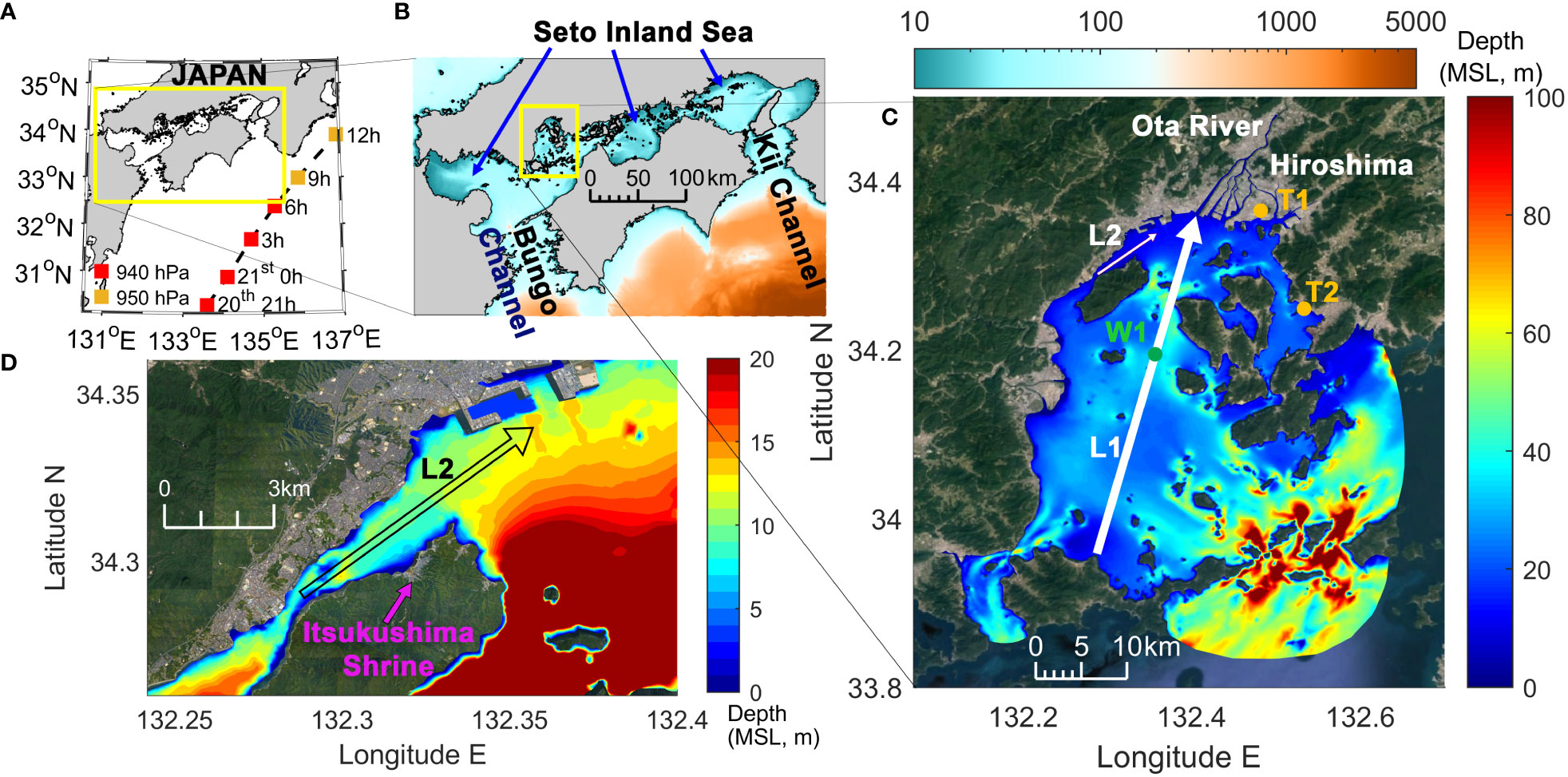
Figure 1 (A) A pathway of Typhoon Roke in 2011, its minimum central pressure, and the location of Seto Inland Sea (yellow box); (B) bathymetry of Seto Inland Sea and the location of Hiroshima Bay (yellow box); (C) bathymetry of Hiroshima Bay and the locations of the Hiroshima and Kure tidal stations, T1 and T2, respectively; and (D) bathymetry near the Itsukushima Shrine and the location of L2.

The Itsukushima Shrine, located in the northern part of the semi-closed Hiroshima Bay in SIS (Figure 1D), is a beautiful and highly cultural-valued structure preserved as one of the World Heritage sites in Japan. The shrine was built by the sea, 30 cm above the highest tide, to prevent it from submerging. However, from 2011 to 2022, the shrine was submerged five times at high tides, mainly in September, due to abnormally high tides in the bay. On 29 September 2011, an abnormally high tide occurred in northern Hiroshima Bay and caused a flooding of the shrine. It was not due to a storm surge because it occurred on a sunny and calm day without distinct atmospheric forcing. A case study for the 2011 flood event based on an acoustic tomography survey postulated that an internal surge caused the northern bay flood. The surge was induced by northerly winds due to the remote typhoon, Roke, passing through the eastern part of the SIS approximately 400 km east of Hiroshima Bay (Zhang et al., 2014; Zhang et al., 2015a) (Figure 1A). The typhoon had passed east off the bay 7–8 days before the surge. When it approached the SIS the closest, the 10-min mean wind of the typhoon was approximately 49 m/s with a maximum radius of gale wind (approximately 15.4 m/s) of 600 km. Their survey confirmed the upwelling of bottom cold water around the northern part of the bay by the typhoon. Then, the surface temperature that became relatively low by the upwelling was restored to its original warm state after approximately 6 days, whose timescale was in parallel with the sea-level increase. However, even though such sea-level rises have been observed very clearly from tidal stations for several decades (Zhang et al., 2014), its physical generation mechanism on the bay scale still needs to be clarified.

Internal waves as gravity waves within a stratified fluid medium have been studied for their generation process, physical properties, and effects on the environment and ecosystem. Vertical movement by the waves can also cause other accompanying effects, such as the transport of heat and dissolved substances (Wetzel, 2001), resulting in chemical and biological changes in these ecosystems (Lai et al., 2010; Straskraba et al., 2013). In particular, research on internal waves inducing internal surges has been conducted actively in closed or semi-closed systems such as lakes and reservoirs (Lemmin et al., 2005; Roget et al., 2017; Bueno and Bleninger, 2018). Because the internal waves in the relatively stable system are more disruptive, they can easily be observed clearly. Furthermore, the waves can be initiated by diverse forces inducing instability of stratification, for example, turbulence, diffusion, intrusion, bathymetry of the stratified basins, and wind (Bueno and Bleninger, 2018).

In the ocean, research on internal waves is mainly related to the internal tide, which is energetic and periodic (semidiurnal commonly). The internal tide has received highlights due to the dissipation of barotropic tides after interaction with bottom topography. Furthermore, the converted internal tide can enhance vertical mixing (Jithin et al., 2020) by adding baroclinic velocities (Kurapov et al., 2010). In shelf scales, internal waves, excluding internal tides, by winds and freshwater intrusion near river mouths can also generate turbulence and mixing of the stratified water column in internal bores or wind-driven upwelling form (Woodson et al., 2007; Kurapov et al., 2010; Walter et al., 2012).

In semi-closed coastal areas, such as a bay, strait, and fjord, the internal waves in the form of internal seiche can be developed and amplified inside the areas (Otsubo et al., 1991; Suzuki et al., 1997; Arneborg and Liljebladh, 2001; Yamanaka et al., 2011; Castillo et al., 2017). However, as far as the authors are concerned, there is relatively less interest in sea-level variation by internal waves, and no internal surge/seiche-induced abnormal tides and floods in a semi-closed bay are reported. Thus, we investigate the physical process of abnormal tides and floods due to the internal surge to find evidence of internal waves in Hiroshima Bay to explain the process of abnormal sea-level rises several days after the passage of typhoons. Also, this research will be helpful for the environmental management of the bay with Japan’s largest oyster aquaculture industry.

In this study, first, we attempted to verify the internal surge suggested as the cause of the flooding by Zhang et al. (2014) and Chen et al. (2017) and then investigate the density-driven circulation using vertical and horizontal current and density profiles at the scales of the Hiroshima Bay and the Itsukushima Shrine. Finally, we explain the bay-scale generation mechanism of the internal surge, consequential abnormal high tide, and flood of the shrine. To achieve those objectives, a high-resolution unstructured-grid 3D ocean circulation model for Hiroshima Bay was established, and its simulation results were validated with observations.

2 Material and methodology

2.1 Outline of numerical model: SCHISM

Semi-implicit Cross-scale Hydroscience Integrated System Model (SCHISM) was applied to simulate the development process of internal waves under the effect of a remote typhoon in Hiroshima Bay. The unstructured-grid 3D baroclinic finite element model, SCHISM, is an open-source and derivative product based on the original SELFE [v3.1dc; Zhang and Baptista (2008)] (Zhang et al., 2016). The latest version of the SCHISM model is capable of following (1) mixed triangular–quadrangular horizontal grid useful to describe complicated coastal lines; (2) semi-implicit finite-element/-volume method to solve the Navier–Stokes equations in hydrostatic form to embrace extensive physical and biological processes; (3) a higher-order scheme for the momentum advection with ELAD filter to control excess mass with an iterative smoother; (4) a higher-order implicit advection scheme for transport (TVD²) using two limiters (in space and in time), which helps the successful capture of smaller eddies by conserving baroclinic instability without filtering out; (5) a highly flexible vertical grid system of the Localized Sigma Coordinates with Shaved Cells (LSC²), which makes it possible to significantly reduce pressure gradient errors by making a coordinate slope much milder than in terrain-following coordinates (Zhang et al., 2015b); and (6) a new horizontal viscosity scheme, which is less dissipative in the eddying regime, with a purpose of efficiently filtering out spurious inertial modes without introducing excessive dissipation. These strengths of SCHISM allow seamless cross-scale modeling across creek–lake–river–estuary–shelf–ocean scales.

The fundamental equations for the hydrodynamic model, SCHISM, are the continuity equation, the momentum equation, and the transport equation in sequence:

$\begin{array}{ll}\nabla ·u+\frac{\partial w}{\partial z}=0& (1)\end{array}$

$\begin{array}{ll}\frac{Du}{Dt}=\frac{\partial }{\partial z}(\nu \frac{\partial u}{\partial z})-g\nabla \eta +F& (2)\end{array}$

$\begin{array}{ll}\frac{DC}{Dt}=\frac{\partial }{\partial z}(\kappa \frac{\partial C}{\partial z})+F_h+Q & (3)\end{array}$

where ($x$, $y$) are the horizontal Cartesian coordinates, $z$ is the vertical coordinate (upward), $t$ is the time, $u$ ($u$ , $y$ , $z$ , $t$) is the horizontal velocity, $w$ is vertical velocity, $h$ ($x$ , $y$) is the bathymetric depth, $\eta$ ($x$, $y$, $t$) is the free surface elevation, $\nabla$ is $(\partial /\partial x, \partial /\partial y)$, $D/Dt$ is material derivative, $g$ is the acceleration of gravity [m s⁻²], $C$ is tracer concentration (e.g., salinity, temperature, and sediment), $\nu$ is vertical eddy viscosity [m² s⁻¹], $\kappa$ is vertical eddy diffusivity for tracers [m² s⁻¹], and $F$ is other momentum forcings such as Coriolis, air pressure, horizontal viscosity, and earth tidal potential. $F_h$ is horizontal diffusion, and $Q$ is mass sources/sinks of tracers.

The wind stress vector (${\tau }_{wx}$, ${\tau }_{wy}$) was parameterized as described in Pond and Pickard (1998):

$\begin{array}{ll}{\tau }_{wx}= C_{wD}\times {\rho }_a\times W_m\times W_x& (4)\end{array}$

$\begin{array}{ll}{\tau }_{wy}= C_{wD}\times {\rho }_a\times W_m\times W_y& (5)\end{array}$

where ($W_x, W_y$) are u and v components of the wind at 10 m above the sea surface, its speed is $W_m$ calculated from $\sqrt{W_x^{ 2}+W_y^{ 2}}$, ${\rho }_a$ is the air density (1.293×10^-3 g ml⁻¹ in SCHISM), and $C_{wD}$ is the wind drag coefficient. A regression line to calculate $C_{wD}$ using $W_m$ was proposed by Smith (1980). Thereafter, it was observed that, as $W_m$ increased to 51 m s⁻¹, $C_{wD}$ tended to decrease due to surface bubble layers caused by steep wave faces being sheared off by the wind (Powell et al., 2003). As a result, the regression equation for $C_{wD}$ in SCHISM can be expressed as:

$\begin{array}{ll}{C}_{wD}={1.0}^{-3}\{\begin{array}{c}0.61+0.063\times 6.0 W_m<6.0\\ 0.61+0.063\times W_m 6.0\le W_m\le 50.0\\ 0.61+0.063\times 50, 50.0<W_m \end{array}& (6)\end{array}$

2.2 Model setups

The model was simulated from 17 August 2011 to 9 October 2011 to analyze the abnormal tide on 29 September 2011. The unstructured grid covers Hiroshima Bay from the Ota River with high resolution (10–40 m) to three open boundaries with increasing resolution (650–850 m), as shown in Figure 2. Regarding mesh generation of the bay, pre-defined ocean/land boundaries were used in the Surface-water Modeling System (SMS) software. After several trials, the bias value for the paving mesh type, which controls the mesh density in the domain, was set as 0.055 (default is 0.3) to find the optimal balance between model performance and computing time. As a result, the model consisted of 67,064 nodes and 124,468 cells. Twenty sigma levels were used for the vertical grid. The length scale of the domain is approximately 50 km zonally, 70 km meridionally, 25 m of averaged depth only for the part of the inner bay, and 170 m of maximum depth in the whole domain. The time step was set as 2.5 s by considering the Courant–Friedrichs–Lewy (CFL) condition. At the river boundary for river discharge upstream, the CFL condition showed 0.48 during the simulation, implying that the model is robust enough from unexpected disturbance. As a result, in terms of the computation time, it took approximately 90 min of CPU time to simulate one day with 88 CPUs.

FIGURE 2

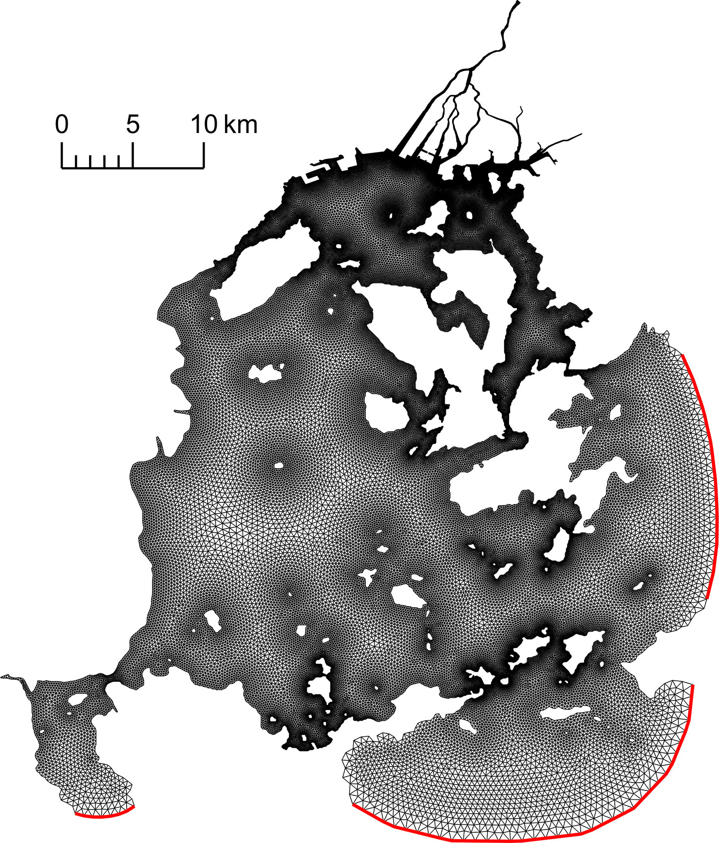
Figure 2 Unstructured grid of Hiroshima Bay for the SCHISM model with open boundaries in red.

For initial and boundary conditions for temperature and salinity, 4D fields from FORA-WNP30 (Four-dimensional variational Ocean Re-Analysis for the Western North Pacific over 30 years; Usui et al., 2017) were utilized. The FORA-WNP30 dataset covers the northwestern Pacific (117°E–160°W, 15°N–65°N) with a horizontal resolution of 0.1° (approximately 10 km) near Japan and 54 vertical levels from 1 m to a maximum of 6,300 m depth. This long-term, high-resolution, and validated FORA-WNP30 is suitable for initial and boundary conditions. The tidal components (M₂, S₂, K₁, O₁, N₂, M₄, K₂, Q₁, and P₁) at the open boundaries were derived from the FES2014 oceanic tide model (Carrère et al., 2015).

2.3 Forcing data

Observing sea surface elevation from tidal stations in the model domain was used to validate model performance. The data were obtained from Hiroshima and Kure tidal stations, shown as T1 and T2 (Figure 1C). To remove possible perturbation of sea level due to the effect of atmospheric surface pressure, the sea-level data were corrected with a conversion rate of 0.01 cm/Pa, as done by Zhang et al. (2014). The temporal resolution of tide observation was 30 s; thus, 20 observations were averaged to obtain 10-min averaged tidal levels, the same time interval as the numerical model results. All datasets used for this research are summarized in Table 1.

TABLE 1

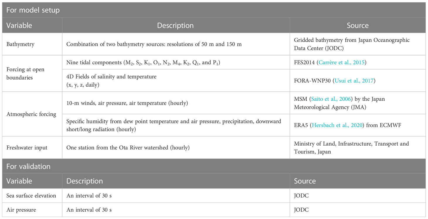
Table 1 Datasets used to set up and validate the hydrodynamic model of Hiroshima Bay.

For bathymetry of the computational domain, two datasets with different spatial resolutions were considered and merged: 50 m and 150 m from Japan Oceanographic Data Center (JODC). Since the 50-m-resolution bathymetry does not cover the whole model domain, the 150-m-resolution data were merged for the areas where the 50-m-resolution data are unavailable to describe bathymetry precisely as much as possible with available datasets.

To consider the effects of the Ota River discharge on the complex circulation of the bay, the bathymetry of the river mouth was reconstructed by utilizing the information of six heights of watermarks from zero elevation at six water level gauges from the river mouth along the Ota River. The water level gauge data were retrieved from the Disaster Prevention Information for River (www.river.go.jp) of the Ministry of Land, Infrastructure, Transport and Tourism (MLIT). The heights of the river bottom were calculated from the heights of watermarks distributed from the river mouth to the upper river, then interpolated to the model mesh by assuming that the bathymetry of the river would become shallower smoothly and gradually upstream.

For the Ota River discharge, hourly discharge information at Yasuohashi and Yagucghidaichi hydrological observatories in the Ota River from the Water Information System (www.river.go.jp) of MLIT was used. If the discharge data include sinusoidal patterns from the tide, the discharged water may be brackish rather than pure freshwater, which we need to input. Therefore, the observatories were selected since they are located enough upstream and then confirmed that tidal effects can be negligible.

For surface atmospheric forcing, such as surface winds at 10 m, air pressure, air temperature, specific humidity, precipitation rate, and downward long- and short-wave radiations, two datasets, Meso-Scale Model (MSM: Saito et al., 2006) by the Japanese Meteorological Agency (JMA) and ERA5 (Hersbach et al., 2020) operated by the European Centre for Medium-Range Weather Forecasts (ECMWF), were used.

The MSM results are an hourly dataset covering Japan and its environs (22.4–47.6 N and 120–150 E) with a resolution of 0.0625° zonally and 0.05° meridionally (approximately 5 km). In 2011, the MSM had forecasted 33 h at 03, 09, 15, and 21 UTC and 15 h at 00, 06, 12, and 18 UTC (the ranges are extended steadily so far. Thus, 78 h at 00 and 12 UTC and 39 h at 03, 06, 09, 15, 18, and 21 UTC are being forecasted from June 2022). To make a continuous hourly dataset, we retrieved 10-m surface winds, atmospheric temperature, and an atmospheric pressure of 2–13th hours from the model forecasted every 00 and 12 UTC. The extracted fields from MSM were adopted as the main surface atmospheric fields because MSM is a regional model with a higher resolution than ERA5.

The other forces, such as downward long- and short-wave radiations, precipitation rate (kg m⁻² s⁻¹), and surface-specific humidity, were extracted from ERA5 because these were not available from MSM. The specific humidity was calculated by

$\begin{array}{ll}{q}_v=0.622\frac{e}{p}& (7)\end{array}$

$\begin{array}{ll}e=611\times \exp (\frac{17.27*T_d}{237.3+T_d})& (8)\end{array}$

where $e$ is vapor pressure, $p$ is air pressure, and $T_d$ is dew point temperature. The extracted fields from ERA5 were interpolated onto the MSM model grid to define all atmospheric forces from different models on the same grid.

3 Results

3.1 Validation: tides

The model results of surface elevation were validated against the observed tide levels at T1 and T2 (see Figure 1C) from 17 August to 9 October 2011. Figure 3 presents the results focusing on the critical research periods: typhoon season and abnormal tide. At T1, the model showed an R² of 0.96 and an RMSE of 0.18 m with observation. The tide at T1 showed the characteristics of a mixed, predominantly semidiurnal tide during the neap tide and a semidiurnal tide during the spring tide. The amplitudes of tidal constituents were 1.01 m, 0.42 m, 0.31 m, and 0.29 m for M₂, S₂, K₁, and O₁, respectively. The maximum range of spring tides during the simulation was 3.85 m on 30 September. Sea-level elevation at T2 also showed a high R² of 0.94 with observation and RMSE of 0.22 m. The model well simulates astronomical tides, both amplitudes and phases, in the computational domain.

FIGURE 3

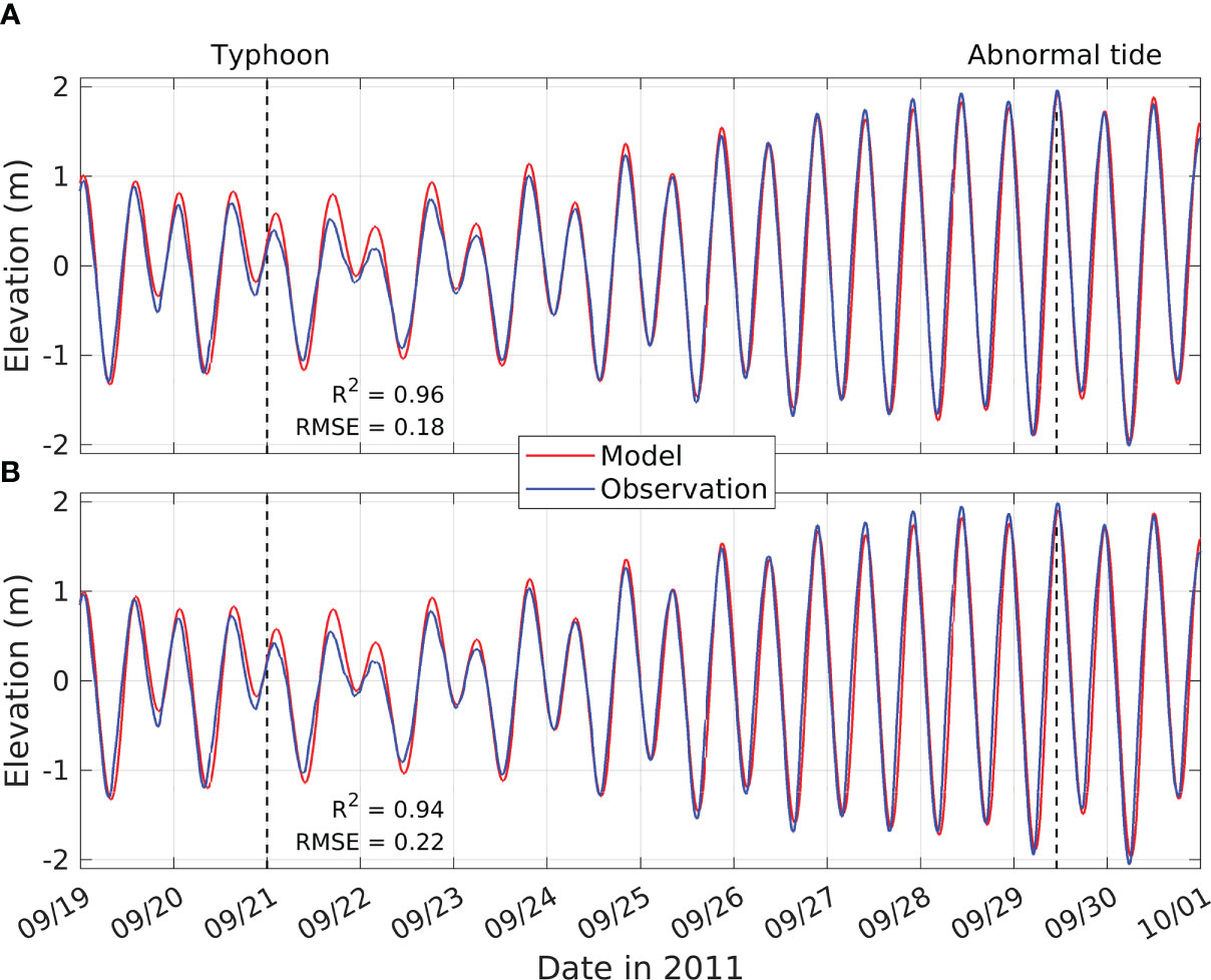
Figure 3 Time series of sea levels from model results (red) and observations (blue) at (A) T1 and (B) T2 for the simulation period (see Figure 1C for the locations of the tidal stations). Two vertical dotted lines indicate the moments the Typhoon Roke passed (left) and the abnormal tide occurred (right) in 2011.

For almost all structures near coastal lines, theoretically possible high tide level, the highest astronomical tide level, was already considered in their construction processes to prevent floodings. However, when the abnormal tide occurred on 29 September 2011, it was a perigean spring tide with an amplitude of approximately 2 m. Considering that spring high tides showed an amplitude of 1.5 m and neap tides had an amplitude of approximately 0.5 m, the structures became more vulnerable to flooding by seawater during the perigean spring tide.

Although tides based on tidal constituents can be predicted accurately, subtidal components of surface elevation can make further rises unpredictable. To extract subtidal components of the elevation, a second-order band-pass Butterworth filter with cutoff periods of 4 and 15 days was applied to the time series from T1, shown in Figure 4. Before applying the filter, missing data around September 14 (not shown) were replaced with reconstructed astronomical tide components predicted using T_TIDE and T_PREDIC by the T_Tide Harmonic Analysis Toolbox (Pawlowicz et al., 2002) to avoid possible errors in the filtering process. The replaced observation time series used for the filter was shown as a gray-colored time series in Figure 4A. On 2 and 21 September, northern winds prevailed in Hiroshima Bay. When there were wind fluctuations, the filtered observation showed variation accordingly, even though these amplitudes were irregular from 3 cm to 9.3 cm (Figure 4A). The subtidal component of observation increased before the relatively strong winds and then decreased under the direct effects of the winds. After that, residual fluctuations remained for about 10 days.

FIGURE 4

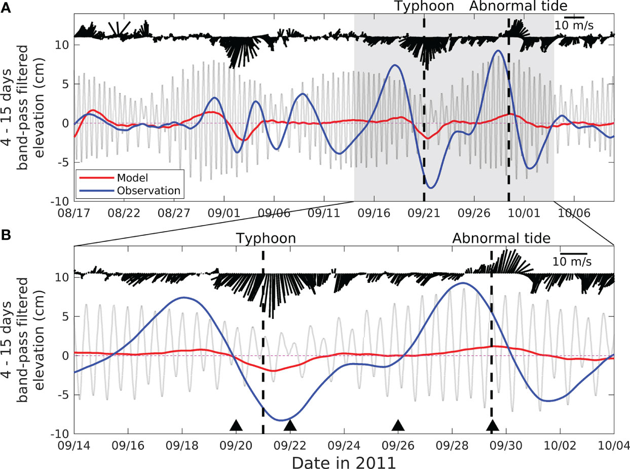
Figure 4 (A) Four to 15 days band-pass-filtered sea level from model results (red) and observed elevation (blue) at T1 in Figure 1C. (B) Close-up focusing on the research period. Black vectors indicate surface winds at W1 in Figure 1C. Gray time series are the original observation before filtering depicted to illustrate the sequence of neap and spring tides.

Regarding phase, the model results also showed similar fluctuations with the observation. However, these amplitudes were relatively smaller than those of the observation. The second northernly wind on 21 September during a neap time was due to Typhoon Roke passing far east off the bay. The northerly wind decreased the subtidal component by 8.3 cm in sea level at T1 in northern Hiroshima Bay (Figure 4B). Then, after 8 days, the neap tide became a spring tide, and the subtidal component increased up to 9.3 cm. These overlapped potentials of increase (including the effect of thermal expansion during summer; Zhang et al., 2016) made the Itsukushima Shrine vulnerable to flooding by seawater. The model results also showed an in-phase decrease of 2.0 cm and an increase of 1.2 cm during the remote typhoon passage and after 8 days, respectively. However, these amplitudes of the variation from the model had approximately 13%–24% of those from the observation.

The same filter was applied to the entire model domain to compare spatial differences of the surface elevation in Hiroshima Bay. The four most appropriate times, indicated in Figure 4B, were selected to present the effects of the typhoon in 2011 in Figure 5. Just before the typhoon passed (Figure 5A), the filtered elevation started to decrease to −0.5 cm (+0.5 cm) near the northern (southern) part of the bay. After 2 days, the northern winds caused by the typhoon transported the seawater toward the south and induced a wind setup. The wind setup reached about −2 cm at T1 and −1.33 around the Itsukushima Shrine, as the same signal from the filtered time series can be found in Figure 4B. This decrease in elevation is shown on a scale of the whole of Hiroshima Bay. Hence, it is not a local phenomenon near the shrine. As the wind diminished about 4 days after the typhoon, the displacement disappeared, as shown in Figure 5C. Then, on 29 September 2011, the sea level increased unexpectedly by approximately 1.5 cm concentrating on the northern part of the bay. These temporal displacements during and after the typhoon imply the bay-scale seesaw-like oscillations (internal waves) in Hiroshima Bay. There are distinctively positive and negative values between islands (34°N, 132.5°E) on 22 and 29 September, respectively. A bottleneck phenomenon of seawater caused these. On 22 September (Figure 5B), the seawater concentrated by the wind setup tried to get out through narrow passages between islands. This rush of seawater induced an increase in sea levels. On the other hand, the sea level decreased near the northern part of the bay on 28 September. Hence, seawater outside the bay tended to be sucked into the bay, which was captured in Figure 5C. One more outstanding value near the open boundary was due to the depth shallower than the surrounding areas (see Figure 1C for the bathymetry).

FIGURE 5

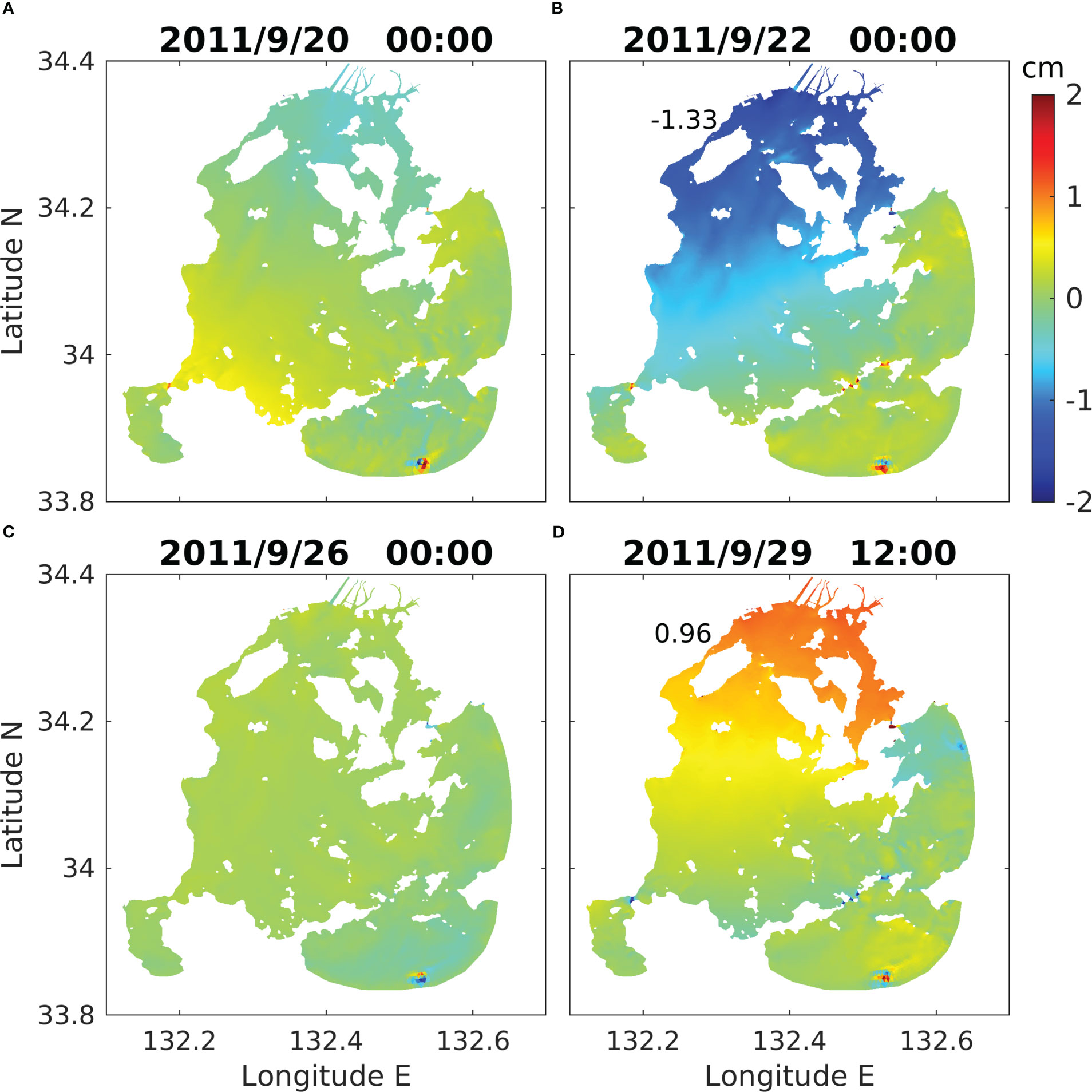
Figure 5 Band-pass [4–15 days]-filtered surface elevation distributions from the model results. (A) Just before the remote typhoon passage, (B) just after the typhoon passage, (C) 2 days after the typhoon passed, and (D) when the abnormal tide occurred. Wind vectors at each corresponding time are indicated with black triangles at the bottom in Figure 4B. The numbers in (B, D) indicate the heights of sea level decrease and rise at the Itsukushima Shrine, respectively.

3.2 Kinetic energy of an internal wave

To calculate and visualize an internal wave quantitatively, the depth-integrated horizontal kinetic energy of the internal wave was calculated (Jeon et al., 2019). The equation used in this study is

$\begin{array}{ll}HKE=\frac{1}{2}{\int }_A^B\rho (z)[u^{\prime }{(z)}^2+v\text{'}{(z)}^2]dz& (9)\end{array}$

where $(u^{\prime }, v^{\prime })$ is zonal and meridional velocity filtered in the target wave’s periods (4–15 days in this study), A and B are depths of the wave (here, 10–20 m, considering a profile of water density; Zhang et al., 2014), and $\rho$ is the water density. We suggested distributions of the kinetic energy at the four most appropriate periods to grasp the wave pattern in Figure 6. If the depth was shallower than 20 m at a node, the kinetic energy was presented as 0. The vectors in Figures 6B–D indicate the filtered current velocities $(u\text{'}, v\text{'})$.

FIGURE 6

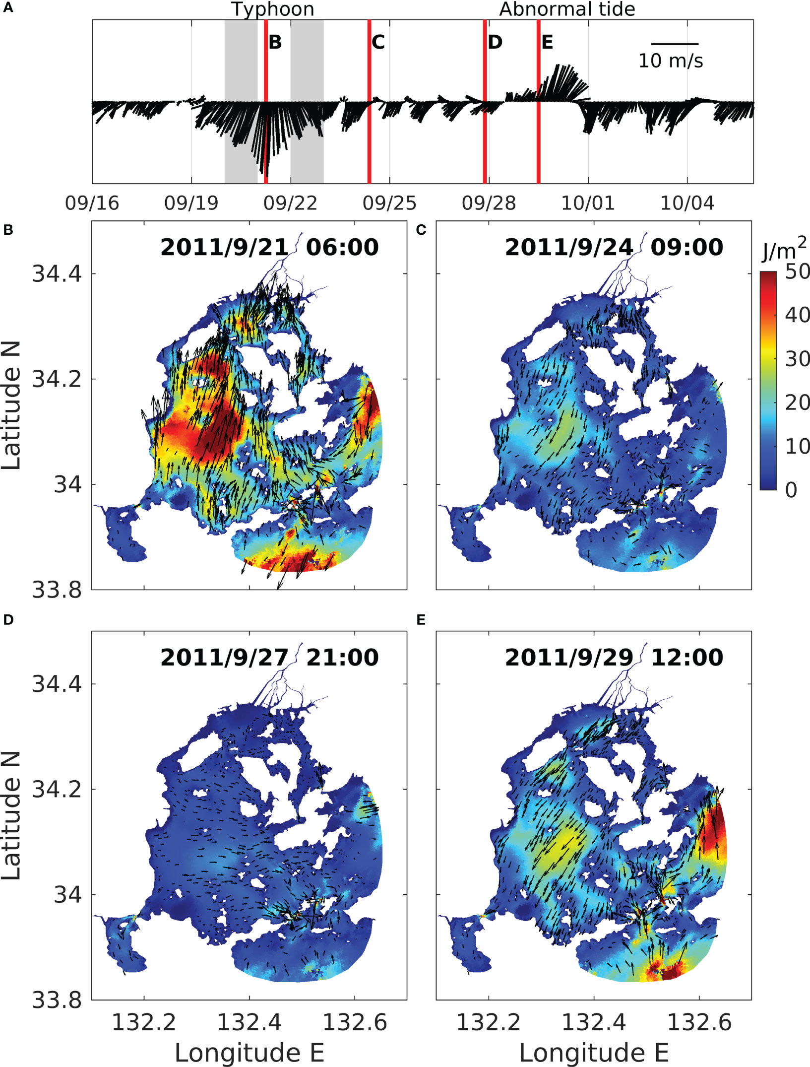
Figure 6 (A) Wind vector at W1 in Figure 1C. Red vertical lines indicate four-time slices for spatial kinetic energy distributions from the model result. Gray areas indicate periods for daily mean calculation used in Figure 7. (B–E) Snapshots of the calculated kinetic energy of the internal wave in Hiroshima Bay at different times.

The typhoon induced intense energy of the internal wave flowing northward, focusing on the central areas of the bay (Figure 6A). In terms of magnitude, the central area has a relatively plain and more expansive topography than the narrow straits between open boundaries and the bay, as presented in Figure 1C. Therefore, it was easier for the seawater in the central area to be transported steadily in one direction without any obstacles like islands or rough topography. This seawater transport allowed the energy to be able to develop. In terms of its direction, the integrated depth (10–20 m) is closer to the ocean bottom than the sea surface because the average depth of the bay is approximately 25 m. Thus, the direction of the filtered velocity at 15 m depth, black vectors in Figure 6, tends to present near-bottom currents, which is usually the opposite direction to the surface winds.

The energy propagation toward the opposite direction (southward) was calculated just after the typhoon passed, as shown in Figure 6B, even though the surface wind was maintained southward. The magnitude of the energy was about half smaller than the energy generated when the typhoon arrived. However, it was a more apparent magnitude than that of the surrounding areas. The same direction of the filtered near-bottom currents and the surface winds implies that other driving forces can exist for the near-bottom currents. As for the possible forces, there is a restoring force. The strongly developed wind set-down in Figure 6B, if the wind got diminished, tended to be increased to recover its equilibrium state. Most of the kinetic energy in the bay diminished after 3.5 days (Figure 6C). On 29 September, the kinetic energy increased again. However, it is thought to be generated by local winds at that time, not the internal wave remaining for a week.

3.3 Density profile and circulation

Through analysis of the transections of daily mean water density and circulation just before and after the remote typhoon passage, density profiles and differences were calculated as a necessary condition of the internal wave. The tidal component was offset by being averaged over two tidal cycles. Two transection lines were decided to include the southern part of the bay and mouth of the Ota River, indicated as L1 in Figure 1C, and to analyze density variation along the narrow channel between the Itsukushima Shrine and the mainland, indicated as L2 in Figure 1D.

Figure 7 shows the meridional transection profiles along the L1. Before the typhoon sufficiently affected Hiroshima Bay, the stratification in the bay was stable, as shown in Figure 7A. In the center of Hiroshima Bay, there was a vertical density difference of approximately 1 kg m⁻³. A much stronger density stratification was distributed near the Ota River mouth due to the influence of freshwater inflow. In the case of cross-sectional flow velocity, the surface velocity flowed southward under the direct influence of the northerly wind. As a result, the northward flow was developed in the sub-surface and bottom layer opposite the surface flow. Immediately after the bay had undergone the direct influence of the typhoon, the stable density profile (stratification) before the typhoon passage disappeared with a decrease in the vertical difference of water density to 0.2–0.4 kg m⁻³. In particular, the seawater in Hiroshima Bay showed a vigorous vertical mixing, resulting in the isopycnic having a columnar shape in Figure 7B. The density difference before and after the typhoon passage was calculated to identify the temporal change in seawater density, as presented in Figure 7C. The typhoon induced an overall increase in vertical mixing. Therefore, the surface density increased by 0.5 kg m⁻³, and the near-bottom density decreased by up to 0.3 kg m⁻³ locally. In particular, the counterclockwise circulation caused by the northerly wind resulted in the distinguishable decrease near the bottom at the southern part of the bay.

FIGURE 7

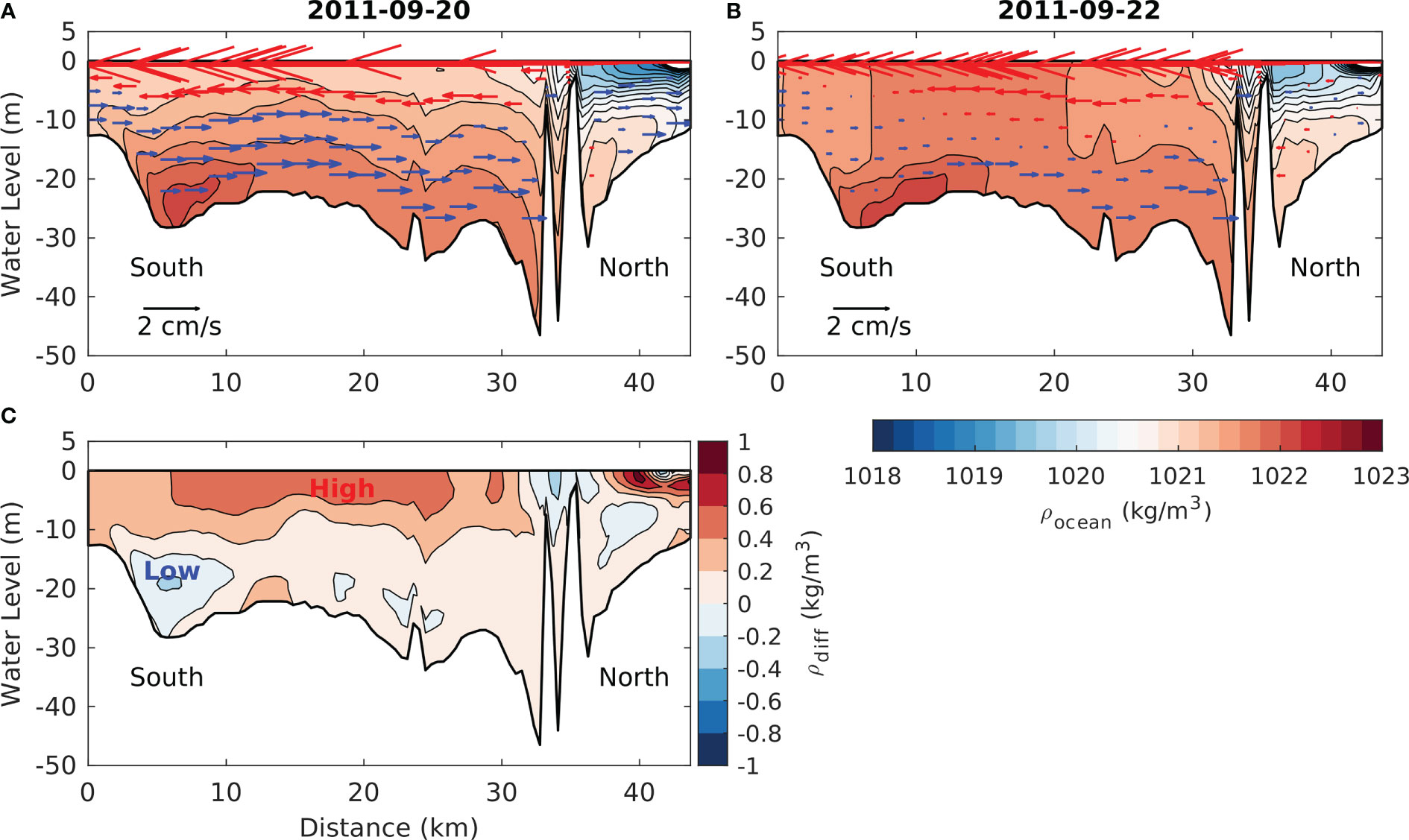
Figure 7 (A, B) Transects for the daily mean density profile and circulation from the model result along L1 (see Figure 1). Daily mean periods are indicated in Figure 6A. Vectors indicate currents toward the south (north) in red (blue). (C) A transect for the density difference between (A, B).

Figure 8 shows the transection profiles along L2. The L2 line includes the adjacent sea of the Itsukushima Shrine, connecting the narrow channel in front of the shrine and the river mouth of the Ota River. Overall, seawater density was lower than that in the central bay (compare Figure 7A and Figure 8A) because of the freshwater from the Ota River. The freshwater near the surface layer enhanced the stratification with a vertical density difference of approximately 1.6 kg m⁻³ (Figure 8A). During the typhoon’s passage, the low-density surface water converged horizontally towards the gradually narrowing strait (see Figure 1D), and the seawater was strongly mixed vertically in the strait. As a result, seawater density became low in front of the shrine (2 km to 4 km in Figure 8B). Based on the vertical current profile, the right river side showed clockwise circulation, and the left showed counterclockwise circulation because of a symmetrical water density distribution. The lower denser water fed into the strait, contributing to the abnormal sea-level rise near the shrine. From the differences in water density in Figure 8C, the near-bottom density at 8 km increased by 0.3 kg m⁻³. This heavier seawater at the near-bottom layer came from the central bay, as seen at 40 km in Figure 7C. The right sides of both Figures 7 and 8 are close to each other.

FIGURE 8

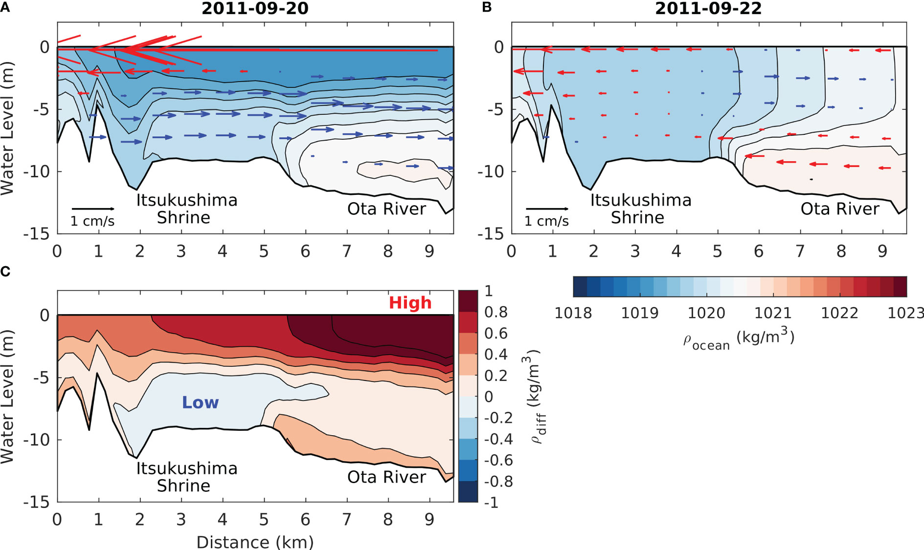
Figure 8 (A, B) Transects for the daily mean density profile and circulation from the model result along L2 (see Figure 1). Daily mean periods are indicated in Figure 6A. Vectors indicate currents toward the Itsukushima Shrine (Ota River) in red (blue). (C) A transect for the density difference between (A, B).

The stratification that became unstable tends to restore its original state. In this process, internal waves are easily generated below the sea surface. From the simulation results and analysis, we confirmed the tendency of the stable stratification to become unstable within 2 days under the direct influence of the remote typhoon passage. This implied that a typhoon passing east off the bay could more likely cause internal waves under the strong stratification.

4 Discussion

Regarding the filtered sea-level variation, which causes the abnormal tide, the simulated subtidal component was relatively lower than the observed one, as previously described.

Sensitivity tests were conducted on typhoon winds and density stratification to investigate which factor can affect the abnormal tide more. Four cases were tested and compared to each other, including a control case with the original forcings and three experimental cases. For a stratification case, the surface and bottom seawater density difference was enhanced approximately three times from 2 kg/m³ to 6 kg/m³. The TS diagram in Figure 9 shows the distribution of the original seawater density at the surface (25%) and bottom (25%) layers. To give more distant values than the control case, 27°C and 30 PSU were given for the surface (above 12.5 m depth), and 18°C and 34.6 PSU were given for the bottom (below 12.5 depth). For two wind sensitivity cases, 50% and 150% of wind speed were considered during the typhoon season from 19 September 2011, 00:00 to 19 September 2011, 12:00 (red and green vectors, respectively, in Figure 10). The real typhoon induced northerly winds with a wind speed of 15 m/s at its peak. Thus, approximately 22.5 m/s and 7.5 m/s were given as the amplified and reduced cases.

FIGURE 9

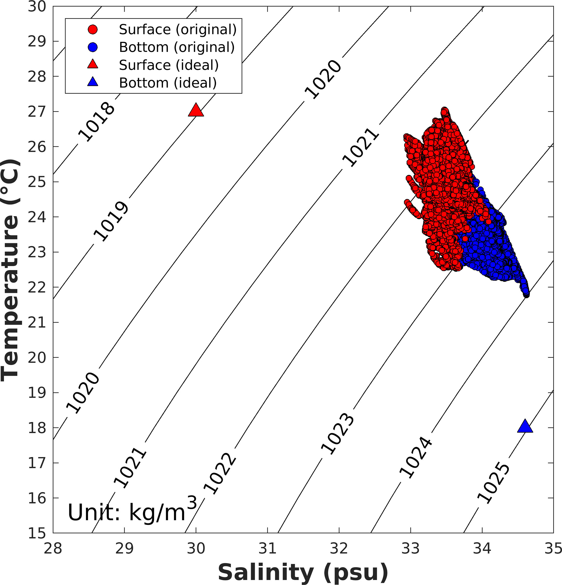
Figure 9 TS diagram for the surface (red) and bottom (blue) seawater at the open boundaries. Circular points are from the original case, and triangular points are the conditions considered in the stratification sensitivity experiment.

FIGURE 10

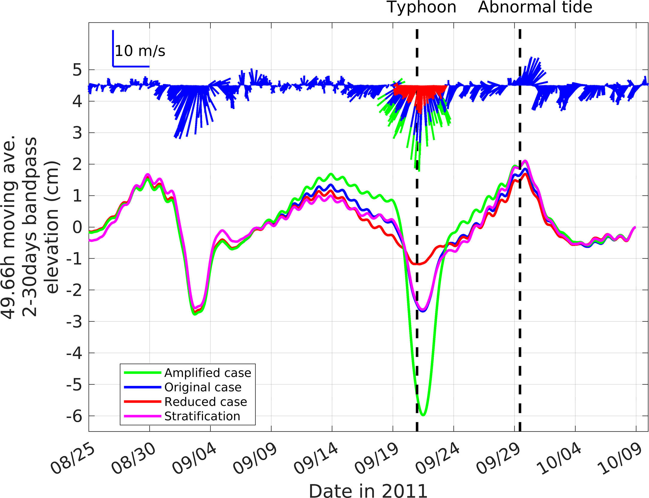
Figure 10 Comparison of subtidal component elevations among sensitivity cases at T1.

From three sensitivity cases, subtidal components using two tidal-cycle moving averages and [2–30 days] band-pass filter were derived and compared with the result from the original case, as shown in Figure 10. Owing to the ringing effect of the filtering method, some differences can be found even before the different forcing was given near the sharp minimum levels on 21 September 2011. However, it should be noted that the ringing effect does not affect the results and interpretation of the sensitivity tests. In the test results with surface wind forcing, the filtered sea level depicts the direct responses to the winds. In the amplified case, the intensified winds transported the surface seawater southward more, resulting in the sea-level decrease of 6 cm due to wind set-down, which is more than two times larger than the original case. In the reduced case, the decreased winds during the peak decreased the sea level by 1 cm, approximately two times smaller than the original result. In the stratification case, the result was almost similar to the original case during the typhoon passage.

After 8 days, when the abnormal tide occurred around 19 September 2011, the amplified and stratification cases showed increments in the filtered sea levels. Notably, the stratification case exhibited a higher increment in the sea level. However, considering the possible error range of 5% in resulting sea levels, there are no significant differences among all cases. It means the typhoon can trigger internal waves in Hiroshima Bay by inducing wind setup and disturbance of stratifications. However, it might not be enough to explain all phenomena occurring in this bay. Other factors besides the internal wave that can amplify the abnormal tide would exist and be explored.

5 Conclusions

The Itsukushima Shrine, built over water, has been flooded by seawater even though the height of the shrine’s floor is 30 cm higher than the highest astronomical sea level. These unexpected floodings, called abnormal tides in this study, usually occurred in late September or early October and recently happened five times over 12 years from 2011. Usually, floodings caused by storm surges and wind setup happen during a typhoon’s passage. However, in the case of 2011, it occurred 9 days after the passage of Typhoon Roke. The weather at that time was partly sunny; therefore, it was difficult to predict the abnormal tide.

We adopted SCHISM to reproduce the abnormal tide in Hiroshima Bay since this model’s unstructured grid and seamless cross-scale modeling allowed us to describe narrow and complex straits between islands and tributaries of the Ota River. During 54 days of the simulation, tides, seawater density, river discharge, and atmospheric forces were used as initial and boundary conditions.

In Hiroshima Bay, the tidal range during spring tide increases to 4 m. The simulation reproduced the spring and neap tides well, and the surface elevation was validated at T1 and T2. Compared to the observed one, the model results showed R² values of 0.96 at T1, located in a downstream area of the Ota River, and 0.94 at T2, located inside complicated islands.

The subtidal components of surface elevation extracted by a band-pass filter showed decreasing tendency according to the typhoon’s approach in both observation and the model results. Then, they showed increases 9 days after the typhoon’s passage, called the abnormal tide, in this study. These increases and decreases in elevation observed at T1 did not happen locally, only near the station. In the simulation, we could find that the oscillation was occurring over the whole of Hiroshima Bay, even though only 13%–24% of the amplitude was calculated compared to the observed amplitude.

At the same time, the typhoon also affected currents and density stratification under the surface. As a result, the kinetic energy of the currents filtered with periods of the internal wave developed, and the stable stratifications in Hiroshima Bay and near the Itsukushima Shrine were mixed, especially vertically, under the effect of the typhoon. It means that the disturbed stratification could trigger the initiation of internal waves. Therefore, the kinetic energy of those energies also increased. However, the energy was not maintained until the abnormal tide actually occurred.

Sensitivity tests were conducted to determine which factor closely relates to the abnormal tide. During the typhoon season, as the intensity of the winds becomes 150%, the sea level decreases due to wind setup becoming more than 200% larger. When the abnormal tide occurred, there was no distinct difference between the original case, cases in the winds changed, and a case in stratification was strengthened. It can imply that other factors that can amplify the abnormal tide in the bay may exist and has to be further studied.

The SIS enclosing Hiroshima Bay has a unique ocean environment. Many people work in diverse industrial activities along the complex coastlines, and much effort is being made to preserve the historical heritage. However, since the abnormal tide is sensitive to changes in absolute sea level, if the global sea-level rise intensifies, the abnormal tide could occur more frequently in the future. This study will help us to understand the generation process of flooding in detail and, furthermore, to be able to establish adaptable policies or strategies to respond to the flooding.

We conducted numerical simulations of the internal wave in Hiroshima Bay to investigate physical processes occurring on the bay scale. However, our simulation could reproduce only 20% of the subtidal sea-level rise 9 days after the typhoon’s passage. The SIS, including Hiroshima Bay, also has oceanic characteristics distinct from those of the Pacific Ocean due to its narrow channels connecting the SIS and the Pacific Ocean. Therefore, SIS-scale numerical simulation and data analysis will be studied further with the other causes of the abnormal surge and flood in the bay.

Data availability statement

The original contributions presented in the study are included in the article/supplementary material. Further inquiries can be directed to the corresponding author.

Author contributions

J-SJ: Data collection, Numerical modelling, Analysis, Interpretation, Writing-Original Draft, review, editing. HL: Data collection, Analysis, Interpretation, Writing-Original draft, review, editing, Supervision, Funding. NM: Analysis, Interpretation, Writing-Review, editing, Funding. All authors contributed to the article and approved the submitted version.

Acknowledgments

This paper is partially supported by the collaborative research program (2021G-03 and 2023GC-03) of the Disaster Prevention Research Institute of Kyoto University. FES2014 was produced by Noveltis, Legos, and CLS and distributed by Aviso+, with support from CNES (https://www.aviso.altimetry.fr/). The ERA5 was retrieved from the Copernicus Climate Change Dataset of ECMWF and modified by interpolation and calculation for the demanded variables of SCHISM.

Conflict of interest

The authors declare that the research was conducted in the absence of any commercial or financial relationships that could be construed as a potential conflict of interest.

Publisher’s note

All claims expressed in this article are solely those of the authors and do not necessarily represent those of their affiliated organizations, or those of the publisher, the editors and the reviewers. Any product that may be evaluated in this article, or claim that may be made by its manufacturer, is not guaranteed or endorsed by the publisher.

References

Arneborg L., Liljebladh B. (2001). The internal seiches in gullmar fjord. part I: dynamics. J. Phys. Oceanogr. 31, 2549–2566. doi: 10.1175/1520-0485(2001)031<2549:TISIGF>2.0.CO;2

CrossRef Full Text | Google Scholar

Bueno R., Bleninger T. (2018). Wind-induced internal seiches in vossoroca reservoir, PR, Brazil. RBRH 23, e25. doi: 10.1590/2318-0331.231820170203

CrossRef Full Text | Google Scholar

Carrère L., Lyard F. H., Cancet M., Guillot A. (2015). FES 2014, a new tidal model on the global ocean with enhanced accuracy in shallow seas and in the Arctic region. in EGU General Assembly Conference Abstracts, 5481.

Google Scholar

Castillo M. I., Pizarro O., Ramirez N., Cáceres M. (2017). Seiche excitation in a highly stratified fjord of southern Chile: the reloncaví fjord. Ocean Sci. 13, 145–160. doi: 10.5194/os-13-145-2017

CrossRef Full Text | Google Scholar

Chen M., Kaneko A., Lin J., Zhang C. (2017). Mapping of a typhoon-driven coastal upwelling by assimilating coastal acoustic tomography data. J. Geophys. Res. Ocean. 122, 7822–7837. doi: 10.1002/2017JC012812

CrossRef Full Text | Google Scholar

Hersbach H., Bell B., Berrisford P., Hirahara S., Horányi A., Muñoz-Sabater J., et al. (2020). The ERA5 global reanalysis. Q. J. R. Meteorol. Soc 146, 1999–2049. doi: 10.1002/qj.3803

CrossRef Full Text | Google Scholar

Jeon C., Park J.-H., Park Y.-G. (2019). Temporal and spatial variability of near-inertial waves in the East/Japan Sea from a high-resolution wind-forced ocean model. J. Geophys. Res. Ocean. 124, 6015–6029. doi: 10.1029/2018JC014802

CrossRef Full Text | Google Scholar

Jithin A. K., Francis P. A., Unnikrishnan A. S., Ramakrishna S. S. V. S. (2020). Energetics and spatio-temporal variability of semidiurnal internal tides in the bay of Bengal and Andaman Sea. Prog. Oceanogr. 189, 102444. doi: 10.1016/j.pocean.2020.102444>

CrossRef Full Text | Google Scholar

Kates R. W., Colten C. E., Laska S., Leatherman S. P. (2006). Reconstruction of new Orleans after hurricane Katrina: a research perspective. Proc. Natl. Acad. Sci. 103, 14653–14660. doi: 10.1073/pnas.0605726103

CrossRef Full Text | Google Scholar

Kurapov A. L., Allen J. S., Egbert G. D. (2010). Combined effects of wind-driven upwelling and internal tide on the continental shelf. J. Phys. Oceanogr. 40, 737–756. doi: 10.1175/2009JPO4183.1

CrossRef Full Text | Google Scholar

Kurogi M., Hasumi H. (2019). Tidal control of the flow through long, narrow straits: a modeling study for the seto inland Sea. Sci. Rep. 9, 11077. doi: 10.1038/s41598-019-47090-y

PubMed Abstract | CrossRef Full Text | Google Scholar

Lai Z., Chen C., Beardsley R. C., Rothschild B., Tian R. (2010). Impact of high-frequency nonlinear internal waves on plankton dynamics in Massachusetts bay. J. Mar. Res. 68, 259–281. doi: 10.1357/002224010793721415

CrossRef Full Text | Google Scholar

Lee H. S., Kim K. O. (2015). Storm surge and storm waves modelling due to typhoon haiyan in November 2013 with improved dynamic meteorological conditions. Proc. Eng. 116, 699–706. doi: 10.1016/j.proeng.2015.08.353

CrossRef Full Text | Google Scholar

Lee H. S., Shimoyama T., Popinet S. (2015). Impacts of tides on tsunami propagation due to potential nankai trough earthquakes in the seto inland Sea, Japan. J. Geophys. Res. Ocean. 120, 6865–6883. doi: 10.1002/2015JC010995

CrossRef Full Text | Google Scholar

Lee H. S., Yamashita T., Hsu J. R.-C., Ding F. (2013). Integrated modeling of the dynamic meteorological and sea surface conditions during the passage of typhoon morakot. Dyn. Atmos. Ocean. 59, 1–23. doi: 10.1016/j.dynatmoce.2012.09.002

CrossRef Full Text | Google Scholar

Lemmin U., Mortimer C. H., Bäuerle E. (2005). Internal seiche dynamics in lake Geneva. Limnol. Oceanogr. 50, 207–216. doi: 10.4319/lo.2005.50.1.0207

CrossRef Full Text | Google Scholar

Mori N., Takahashi T., Yasuda T., Yanagisawa H. (2011). Survey of 2011 tohoku earthquake tsunami inundation and run-up. Geophys. Res. Lett. 38, L00G14. doi: 10.1029/2011GL049210

CrossRef Full Text | Google Scholar

Otsubo K., Harashima A., Miyazaki T., Yasuoka Y., Muraoka K. (1991). Field survey and hydraulic study of “Aoshio” in Tokyo bay. Mar. pollut. Bull. 23, 51–55. doi: 10.1016/0025-326X(91)90649-D

CrossRef Full Text | Google Scholar

Pawlowicz R., Beardsley B., Lentz S. (2002). Classical tidal harmonic analysis including error estimates in MATLAB using T_TIDE. Comput. Geosci. 28, 929–937. doi: 10.1016/S0098-3004(02)00013-4

CrossRef Full Text | Google Scholar

Pond S., Pickard G. L. (1998). Introductory dynamical oceanography (Burlington, MA, USA: Butterworth-Heinemann).

Google Scholar

Powell M. D., Vickery P. J., Reinhold T. A. (2003). Reduced drag coefficient for high wind speeds in tropical cyclones. Nature 422, 279–283. doi: 10.1038/nature01481

PubMed Abstract | CrossRef Full Text | Google Scholar

Roget E., Khimchenko E., Forcat F., Zavialov P. (2017). The internal seiche field in the changing south aral Sea, (2006–2013). Hydrol. Earth Syst. Sci. 21, 1093–1105. doi: 10.5194/hess-21-1093-2017

CrossRef Full Text | Google Scholar

Saito K., Fujita T., Yamada Y., Ishida J., Kumagai Y., Aranami K., et al. (2006). The operational JMA nonhydrostatic mesoscale model. Mon. Weather Rev. 134, 1266–1298. doi: 10.1175/MWR3120.1

CrossRef Full Text | Google Scholar

Smith S. D. (1980). Wind stress and heat flux over the ocean in gale force winds. J. Phys. Oceanogr. 10, 709–726. doi: 10.1175/1520-0485(1980)010<0709:WSAHFO>2.0.CO;2

CrossRef Full Text | Google Scholar

Straskraba M., Tundisi J. G., Duncan A. (2013). Comparative reservoir limnology and water quality management (Netherlands: Dordrecht: Springer). doi: 10.1007/978-94-017-1096-1

CrossRef Full Text | Google Scholar

Suzuki T., Matsuyama M., Nagashima H. (1997). Internal near-inertial oscillation in Tokyo bay. Oceanogr. Japan 6, 219–228. doi: 10.5928/kaiyou.6.219

CrossRef Full Text | Google Scholar

Takagi H., Esteban M., Shibayama T., Mikami T., Matsumaru R., De Leon M., et al. (2017). Track analysis, simulation, and field survey of the 2013 typhoon haiyan storm surge. J. Flood Risk Manage. 10, 42–52. doi: 10.1111/jfr3.12136

CrossRef Full Text | Google Scholar

Tollefson J. (2013). Natural hazards: new York vs the sea. Nature 494, 162–164. doi: 10.1038/494162a

PubMed Abstract | CrossRef Full Text | Google Scholar

Usui N., Wakamatsu T., Tanaka Y., Hirose N., Toyoda T., Nishikawa S., et al. (2017). Four-dimensional variational ocean reanalysis: a 30-year high-resolution dataset in the western north pacific (FORA-WNP30). J. Oceanogr. 73, 205–233. doi: 10.1007/s10872-016-0398-5

CrossRef Full Text | Google Scholar

Walter R. K., Woodson C. B., Arthur R. S., Fringer O. B., Monismith S. G. (2012). Nearshore internal bores and turbulent mixing in southern Monterey bay. J. Geophys. Res. Ocean. 117, C07017. doi: 10.1029/2012JC008115

CrossRef Full Text | Google Scholar

Wetzel R. G. (2001). Limnology: lake and reservoir ecosystem. 3rd ed (San Diego: Academic Press).

Google Scholar

Woodson C. B., Eerkes-Medrano D. I., Flores-Morales A., Foley M. M., Henkel S. K., Hessing-Lewis M., et al. (2007). Local diurnal upwelling driven by sea breezes in northern Monterey bay. Cont. Shelf Res. 27, 2289–2302. doi: 10.1016/j.csr.2007.05.014

CrossRef Full Text | Google Scholar

Yamanaka R., Kozuki Y., Miyoshi M., Nogami F., Ishida T., Yamaguchi N., et al. (2011). “Impact of water quality variation on mussel (Mytilus galloprovincialis) biomass,” in Semi-enclosed port (Maui, Hawaii, USA: International Ocean and Polar Engineering Conference).

Google Scholar

Zhang Y. J., Ateljevich E., Yu H.-C., Wu C. H., Yu J. C. S. (2015b). A new vertical coordinate system for a 3D unstructured-grid model. Ocean Model. 85, 16–31. doi: 10.1016/j.ocemod.2014.10.003

CrossRef Full Text | Google Scholar

Zhang Y., Baptista A. M. (2008). SELFE: a semi-implicit eulerian–Lagrangian finite-element model for cross-scale ocean circulation. Ocean Model. 21, 71–96. doi: 10.1016/j.ocemod.2007.11.005

CrossRef Full Text | Google Scholar

Zhang C., Kaneko A., Zhu X.-H., Gohda N. (2015a). Tomographic mapping of a coastal upwelling and the associated diurnal internal tides in Hiroshima bay, Japan. J. Geophys. Res. Ocean. 120, 4288–4305. doi: 10.1002/2014JC010676

CrossRef Full Text | Google Scholar

Zhang C., Kaneko A., Zhu X., Lin J. (2014). Nontidal sea level changes in Hiroshima bay, Japan. Acta Oceanol. Sin. 33, 47–55. doi: 10.1007/s13131-014-0516-4

CrossRef Full Text | Google Scholar

Zhang Y. J., Ye F., Stanev E. V., Grashorn S. (2016). Seamless cross-scale modeling with SCHISM. Ocean Model. 102, 64–81. doi: 10.1016/j.ocemod.2016.05.002

CrossRef Full Text | Google Scholar