SIPN South: six years of coordinated seasonal Antarctic sea ice predictions

1 Introduction

Antarctic sea ice rarely fails to spur our curiosity. By the mid-2000s, sea ice extent anomalies (Figure 1) had exhibited no substantial change despite the global warming context. By contrast, in the Northern Hemisphere, significant reductions in Arctic sea ice extent were already evident year-round (Cavalieri et al., 2003). From 1979 to the mid-2010s, there was a positive trend in Antarctic sea ice extent, leading to a series of hypotheses that could explain such unexpected behavior (see, e.g., Hobbs et al. (2016) for a review). However, in spring-summer 2016-2017, the sign of sea ice anomalies drastically switched from positive to negative, canceling the gradual accumulation that had prevailed since the late 1970s (Parkinson, 2019). Sea ice extent conditions have remained low since then for all months of the year, with an absolute record low set in February 2022 and then in February 2023 (Raphael & Handcock, 2022; Wang et al., 2022; Liu et al., 2023). The interpretation of the summer 2022 and 2023 records is not obvious, given the strong positive phase of the Southern Annular Mode in summer 2021-2022, a mode that is normally associated with positive sea ice extent anomalies (Verfaillie et al., 2022; their Figure S2). Several ocean and atmospheric mechanisms have been hypothesized to explain the 2016-2017 chain of events (Stuecker et al., 2017; Schlosser et al., 2018; Meehl et al., 2019; Purich and England, 2019; Zhang et al., 2022). It is speculated that the recent decline of Antarctic sea ice extent could foreshadow more profound changes in the Southern Ocean system (Eayrs et al., 2021).

FIGURE 1

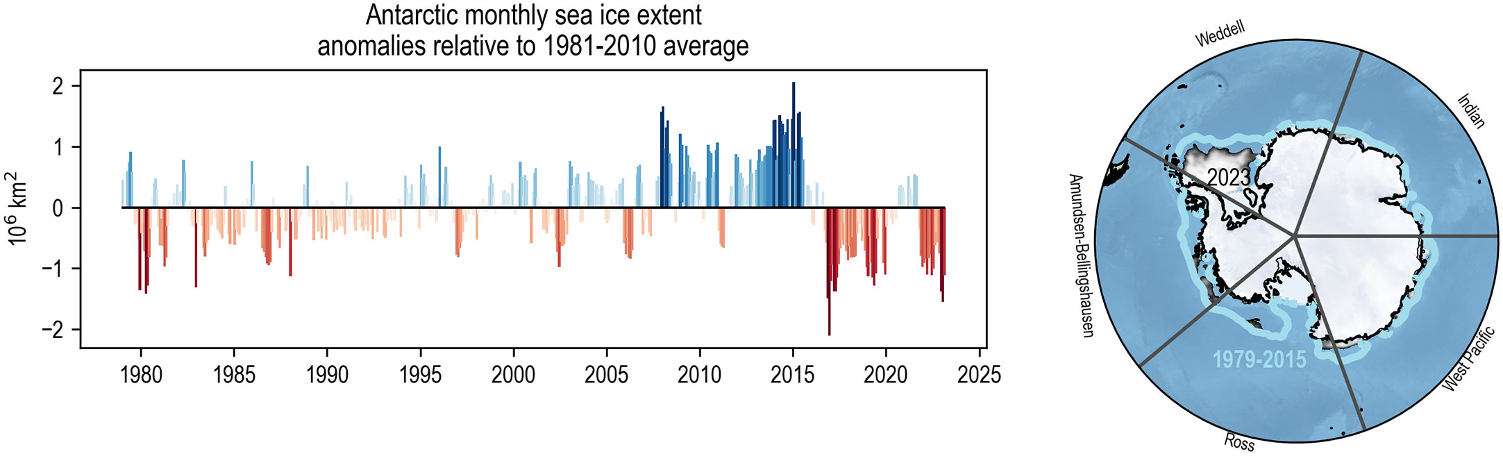
Figure 1 (Left) Antarctic monthly mean sea ice extent anomalies relative to the 1981-2010 mean seasonal cycle, from January 1979 to December 2022 (OSI-SAF sea ice index OSI-420; Lavergne et al., 2019). (Right) The 1979-2015 February climatological sea ice edge, defined as the 15% sea ice concentration contour of the average sea ice concentration field (light blue line), and the February mean 2023 sea ice conditions (white shading). The names of the regions introduced in Section 2.5 are given on this map.

Sea ice is a key variable of the high-latitude Southern Hemisphere. While the Southern Ocean is known as a major carbon sink for the atmosphere, having accounted for up to 40% of the uptake of cumulative anthropogenic carbon emissions (DeVries, 2014), sea ice processes can act both as a source or a sink of atmospheric carbon depending on the season (Delille et al., 2014; Gray et al., 2018). Sea ice growth (melt) is associated with salt (freshwater) fluxes to the upper ocean that directly control its stratification on seasonal to decadal timescales (Martinson, 1990; Goosse and Zunz, 2014; Goosse et al., 2018). Sea ice also dampens horizontal ocean transport processes such as storm-generated waves (Kohout et al., 2014). Recent sea ice loss around the Antarctic Peninsula, for example, has been identified as a possible cause of ice shelf disintegration through enhanced ocean swells (Massom et al., 2018). Finally, sea ice mitigates heat transfers between the ocean and the atmosphere and, as such, plays a key role in the energy balance in polar regions. The year-to-year fluctuations of sea ice at the regional and circumpolar levels might thus have consequences on a longer term and on a global scale. In view of this, the recent sequence of negative anomalies (Figure 1), and our ability to predict these anomalies ahead of time, should be given increased attention.

The interest for sea ice is not limited to the physical environments. Sea ice hosts a stock of bacteria, algae, and grazers which, upon melting, are released in the upper ocean and impact the biological activity including phytoplankton blooms (Brierley and Thomas, 2002). The variations in Antarctic sea ice extent significantly affect marine productivity and fisheries (Liu et al., 2022). Besides, sea ice conditions represent a real risk for all vessels operating in high-latitude marine areas (COMNAP, 2015). This is especially true for commercial operations - most notably fisheries (e.g. krill) and tourism - which tend to use ice-strengthened vessels rather than icebreakers. As the number and variety of tourist activities increase in the high-latitude Southern Ocean (Tejedo et al., 2022), considering sea ice related hazards, even in the middle of austral summer, has become a priority. For all these applications (and many more not mentioned here), a short-term notice (say, a few weeks to months) of the anomalous character of sea ice conditions in a given region would likely represent significant added value over the currently used information that consists of climatological forecasts or interpretation of real-time ice charts. Such information could be valuable as the system appears to be in a non-stationary state where climatology is, by definition, not meaningful.

The feasibility of skillful seasonal sea ice predictions rests on predictability mechanisms operating at sub-seasonal to seasonal time scales. In contrast to historical Arctic sea ice, Antarctic sea ice is almost entirely seasonal and is thinner on average, suggesting possibly different mechanisms. The first estimates of initial-value predictability (i.e., predictability associated with initial conditions or ‘of the first kind’) of Antarctic sea ice are credited to Holland et al. (2013). They investigated the characteristics of an ensemble of sea ice trajectories of the Community Climate System Model version 3 (CCSM3), each initialized on January 1st from the model’s own state but subject to small perturbations at the initial time. They identified an eastward traveling signal of predictability of the Antarctic sea ice edge position with an associated timescale of 3-9 months depending on the region considered. They also noticed a temporary loss of predictability during the ice retreat season followed by an increase in predictability in the second year during the ice advance season. This phenomenon of ‘re-emergence’ of predictability was confirmed in other model setups (Marchi et al., 2019): significant correlations between sea surface temperature (SST) anomalies in two successive winter seasons were diagnosed in a six-model ensemble despite the absence of correlation during summer. The re-emergence phenomenon is explained by the storage of surface information below the ocean mixed layer in the spring and summer seasons and the fact that these anomalies resurface when the mixed layer deepens in autumn and winter. A key finding of the Marchi et al. study is that the predictability horizon appears to be mean-state dependent: climate models with deeper oceanic mixed layers tend to exhibit longer predictability. In an Arctic-Antarctic intercomparison, Ordoñez et al. (2018) showed that Antarctic sea ice area predictability is less influenced by the initial sea ice volume anomalies than in the Arctic. Sea ice predictability is inherently tied to the vertical structure of the properties of the underlying ocean (Libera et al., 2022), which can explain why different estimates of predictability have been obtained with different general circulation models but also why these estimates may vary from one region to another.

In parallel to idealized predictability studies that employ model output without reference to the observed sea ice state, several studies have attempted to determine predictability content using observational and reanalysis datasets or using retrospective predictions (hindcasts). Chen and Yuan (2004) developed the first seasonal forecast for Antarctic sea ice concentration with a statistical model using a reanalysis of atmospheric variables and satellite-observed sea ice data. This linear Markov model showed considerable skill in predicting the anomalous sea ice concentration up to one year in advance in the western Antarctic, and especially high skill in austral winter. Chevallier et al. (2019) estimated that Antarctic sea ice extent anomalies have a typical decorrelation time scale of up to two months in all seasons, except in austral spring (October to December) where it can drop to 3 weeks. Using reanalyses and satellite products, Holland et al. (2017) identified a 5-month relationship between springtime (October) zonal wind anomalies in the Amundsen-Bellingshausen Seas and the March sea ice area in the western Ross Sea: stronger westerlies in spring increase sea ice divergence, favor shortwave absorption and heat storage in the upper ocean and delay autumn sea ice advance. Such a coupled mechanism was, however, not found in state-of-the-art climate models (Holland et al., 2017). Recently, Morioka et al. (2019; 2021) reported skillful prediction of summertime sea ice conditions in the Weddell Sea owing to the initialization of winter sea ice concentration and thickness, pointing to the potentially increased contribution of thickness/volume anomalies to predictability at regional scales. Using a suite of coupled dynamical models, Bushuk et al. (2021) found that predictions of wintertime sea ice edge position are improved when taking into account the zonal advection of upper-ocean heat content anomalies. They also found that the initialization of sea ice concentration and thickness played a key role in summer prediction skill. The Weddell Sea was found to be a hotspot for summertime prediction (up to 9 months out) and less skill was found in the Ross Sea. Payne et al. (2022) also found the largest forecast skill in the Weddell Sea, with moderate skill in the Ross, Amundsen and Bellinghausen Seas, and lowest skill in the Indian and West Pacific sectors. They also found an important role of initial sea ice thickness for August to December predictions. Finally, Zampieri et al. (2019) found that current subseasonal to seasonal (S2S) prediction systems, not specifically geared towards polar prediction, display skill that rarely beats trivial forecasts beyond a few weeks. A key aspect of the Zampieri et al. (2019) study is that they apply a stringent skill metric that penalizes the spatial discrepancies between forecast and observed sea ice edges.

In summary, only a few studies have examined seasonal Antarctic sea ice predictability, and it can be summarized that: (1) predictability estimates vary regionally and seasonally; (2) the upper ocean is key to carrying sea ice predictability over seasons and regions; (3) ocean stratification and the vertical structure of its properties affects estimates of predictability in climate models; (4) predictability and skill are likely conditionally dependent on the baseline mean state; and (5) in model experiments, skill is generally high in the Weddell Sea and varies from one study to another in the Ross Sea. We note that the Weddell Sea is the sector of the Southern Ocean with the largest summer sea ice extent on climatological average. This sector, unlike the others, hosts at least 1 million km² of sea ice every summer, approximately 50% of the circumpolar total (Parkinson, 2019).

The satellite record of observed sea ice extent anomalies (Figure 1) suggests that, since the mid-2000s, Antarctic sea ice could have entered a new regime characterized by increased variance, increased persistence, and lower frequency. From the angle of predictability, the current epoch could well be a ‘window of opportunity’ in which longer-lived sea ice anomalies push the horizon of predictability well beyond the levels that had been prevailing before. Indeed, Payne et al. (2022) showed that hindcast skill increased substantially when the hindcasts include the 2010s.

In that context, the objective of SIPN South is to quantify the skill of the available sea ice prediction systems with a focus on the recent summers. Specifically, we aim to provide an initial answer to three scientific questions:

1. Does the SIPN South ensemble exhibit systematic forecast errors?

2. Do SIPN South forecasts provide added value over a climatological forecast?

3. Is there a relationship between the forecasting approach and skill?

We discuss in Section 2 the SIPN South protocol and the different forecasting approaches taken by the contributors. In Section 3, we attempt to answer the three questions raised above by analyzing the forecasts made from 2017 until 2023. We finish by discussing the limitations of the study and avenues for future work.

2 Methods

We describe the historical context of the SIPN South project and the generic protocol for contributions. Then, we briefly review the different approaches followed by the SIPN South contributors. Finally, we review the products and methods used for forecast verification.

2.1 SIPN South background

SIPN South was initially designed to be a 3-yr (2017-2019) activity taking place within the Southern Hemisphere component of the Year of Polar Prediction (YOPP-SH) project (Jung et al., 2016; Bromwich et al., 2020). SIPN South was created for the scientific reasons described in the introduction, but also to initiate a parallel effort to the (Arctic) Sea Ice Prediction Network (Steele et al., 2021). The project was extended beyond the initial period and now runs every year. SIPN South has briefly been described in Abrahamsen et al. (2020) and Bromwich et al. (2020), and in technical reports published after each forecasting season, all available on the project website (see “Data and code availability” section below).

Around mid-November each year, a call for contributions is issued on various mailing lists related to polar research, and on social media. The call itself contains the protocols to be followed, which we now briefly summarize. The forecasts cannot use data beyond the 1^st of December and must be submitted within the first 10 days of December. The forecasts must cover the period 1^st December to 28^th February (90 days). The method of forecasting is free but must be documented. Up to four diagnostics can be submitted, by order of descending priority and for each of the 90 days of the forecasting period. These diagnostics are: (i) the integrated Antarctic sea ice area, (ii) the sea ice area in each successive 10° longitude band starting from 0°, (iii), the sea ice concentration (provided on the contributor’s native grid), and (iv) the effective sea ice thickness, i.e. sea ice volume per unit grid cell area, also provided on the contributor’s native grid. SIPN South allows the submission of ensembles of forecasts to reflect aspects of uncertainty in the experimental setup. Finally, the call document specifies the two observational products that will be used as references for verification, (see “Observational references” section below).

There are several differences between the protocol followed in the SIPN South protocol and that followed in the (Arctic) sea ice outlooks (SIO) that have been conducted by the Sea Ice Prediction Network (Hamilton and Stroeve, 2016; Steele et al., 2021; https://www.arcus.org/sipn/sea-ice-outlook) since 2008. One difference is the systematic request for daily data in SIPN South (versus monthly in general for the SIO, up to a few exceptions). Having the daily temporal resolution is key to diagnosing the biases that develop at the sub-seasonal time scale, see Section 3.1. Another difference is that SIPN South only issues one call per summer while the Arctic SIO issues four (June, July, August, and September), which allows studying the influence of lead time on the skill. Finally, SIPN South requests explicit probability distributions estimates through individual ensemble members, while the SIO requests aggregated statistics (median and range). Several co-authors of this study are also involved in the SIO and ensure frequent exchanges on best practices in the respective communities.

The year-to-year evolution of the contribution statistics is shown in Figure 2. The latest forecasting exercise documented in this manuscript (2022-2023) has seen a record number of contributions but a slight decrease in the number of files contributed compared to the previous season, due to one group usually contributing more than 50 ensemble members for all diagnostics not being able to submit forecasts for this latest exercise.

FIGURE 2

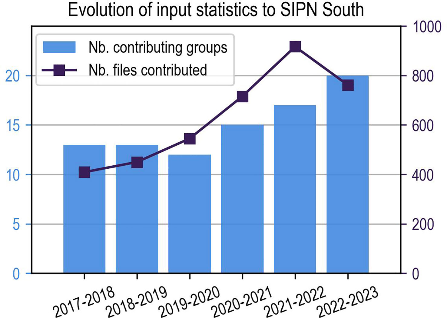
Figure 2 The number of individuals or groups that contributed forecasts to the SIPN South project for each of the austral summers since the beginning of the project (bars, left y-axis) and the total number of files contributed by all groups over the same period (line with squares, right y-axis).

In order to avoid over-interpretation of the results there are four caveats to the structure of SIPN South that need to be acknowledged before any comparison to observations is performed. First, only six years are available, which is very limiting when meaningful statistics need to be drawn. With so few data points, systematic inconsistencies between forecasts and verification datasets can be difficult to detect. Second, an agreement between forecasts and verification data is not a guarantee that the skill is obtained for good reasons. Besides the issue of limited statistical sampling, the SIPN South ensemble can be viewed as an ‘ensemble of opportunity’, i.e., a set of forecasts obtained after asking for output from anyone who is willing to contribute (Tebaldi and Knutti, 2007). The implication is that the range of forecasts contributed to SIPN South is not necessarily representative of the full range of uncertainty for all prediction systems that exist. The results presented here might be updated when more groups contribute to the effort. Third, because forecasting systems are constantly improving and evolving (e.g., physical models, data assimilation methods, observations used, ensemble perturbation methods), contributions labeled identically might correspond to slightly different underlying methods. Finally, no constraint was imposed regarding important aspects that make up prediction systems such as the dataset used for initialization or to train statistical models, the method of ensemble perturbation or uncertainty estimation, the values of specific parameters, or the application of bias correction step. The reason is that SIPN South aims to intercompare prediction systems each with its own design choices. This approach is similar to what has been done in the Arctic SIO (Blanchard-Wrigglesworth et al., 2015; Hamilton and Stroeve, 2016; Blanchard-Wrigglesworth et al., 2023).

2.2 Description of the forecasting systems

Since the approach to forecast is at the discretion of each contributing group, unsurprisingly there is a large variety in the types of forecasting systems used. Other initiatives to collect real-time seasonal predictions like the Seasonal Hurricane Prediction project (https://seasonalhurricanepredictions.bsc.es) and the Arctic Sea Ice Outlook introduced above also face a high diversity in forecasting approaches. For these two projects, forecasts have been categorized as either ‘dynamical’ or ‘statistical’ approaches (Caron et al., 2020; Steele et al., 2021). Dynamical approaches gather predictions made using process-based models, i.e., models based on first physical principles, that are initialized from observationally constrained initial states. These dynamical approaches include general circulation models (GCMs), either only for the ocean (including sea ice) or also coupled to an atmospheric model. By contrast, statistical approaches gather predictions made using data-based models, i.e., exploiting statistical predictor-predictand relationships in past data. This characterization onto dynamical and statistical models could be criticized, since in practice dynamical model predictions are often corrected a posteriori with statistical methods, and statistical forecasts often draw from climate model output or reanalyses to build empirical relationships. A description of the approach followed by SIPN South contributors is given in Table 1. For simplicity, we have assigned a group to ‘dynamical’ approach if it uses a GCM as the foundation of their prediction system, and to ‘statistical’ approach otherwise.

TABLE 1

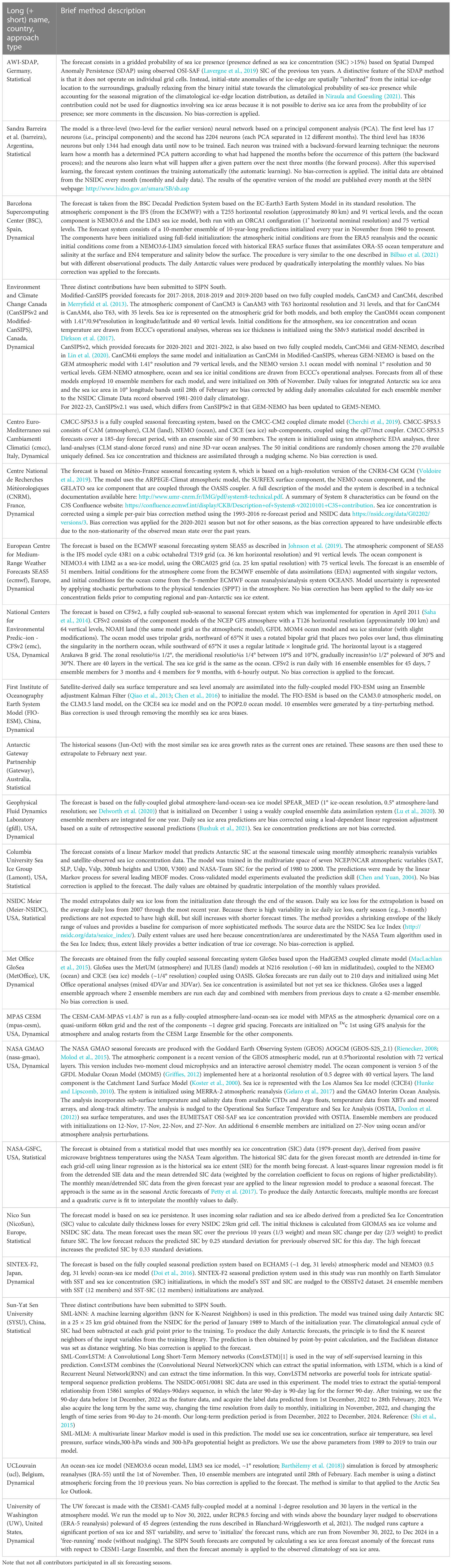
Table 1 List of contributors to the SIPN South austral summer forecasts over the six seasons 2017-2018 to 2022-2023 and description of the method.

A group forecast is finally included in the analyses. The group forecast is constructed as an ensemble forecast of size n with n the number of contributors that provided data for a given year. For contributors providing ensemble members, these ensemble members are first averaged together.

2.3 Observational references

Two observational references were used for verification of the forecasts: the NSIDC-0081 product using the NASA Team algorithm for sea ice concentration reprocessing (Meier et al., 2022) and the OSI-401b product using the Bristol/Bootstrap algorithm (Tonboe et al., 2017). The choice of these products was made based on the near-operational availability of the datasets, but also to test the possible dependence of target diagnostics (sea ice area and concentration) on the choice of the reprocessing algorithms (NASA Team vs Bristol/Bootstrap). Our choice of using two products for forecast verification is motivated by the fact that observational errors introduce variability in skill metrics (Massonnet et al., 2016; Ferro, 2017; Mortimer et al., 2020; Lin et al., 2021).

The two products also display non-negligible differences in land-sea masks: for instance, the area covered by ocean south of 60°S differs by about 7.5% between the two products (46.93 million km² for NSIDC-0081 vs 50.76 million km² for OSI-401b), likely due to differences in spatial resolution and in the treatment of landfast ice and ice shelves. These differences in land-sea masks and in reprocessing algorithms in observational references are to be kept in mind when interpreting SIPN South forecast errors, as these forecast errors can also have a component originating from the verification data itself.

NSIDC-0081 does not extend back prior to 2015 and OSI-401b does not extend back prior to 2005. Long-term climatologies were thus estimated with a third product, namely the OSI-450 dataset (Lavergne et al., 2019) recently superseded by the OSI-450a product, over the period 1979-2015. Note that the estimated climatologies are relatively insensitive to the choice of the observational product (see, e.g., Figure 1A of Roach et al. (2020) or Figure 3B of Lin et al. (2021)).

2.4 Climatological forecast

When assessing forecast skill, it is advisable to define a benchmark forecast (also known as the ‘baseline’ or ‘reference’ forecast) that is cheap to construct. The goal of such a benchmark forecast is to help establish whether the other forecasts outperform a naive prediction. In our case, the benchmark forecast is defined as the climatological forecast, comprising a 30-member ensemble corresponding to the 30 sea ice states of the 30 years preceding the target season. For example, the benchmark forecast for the 2020-2021 December-January-February forecasting season consists of the observed sea ice areas and concentrations of the December-January-February 1990-1991, 1991-1992, … 2019-2020 seasons. The climatological forecast is based on the OSI-401b product of sea ice concentration after 2015, and on the OSI-450 product before 2015. It is labeled “climatology” in the figures.

We are aware that other benchmark forecasts could have been introduced at this stage, such as: the trend extrapolation (sea ice area at day D is extrapolated from the linear or quadratic trend fitted to the previous areas at day D from previous years), the persistence forecast (sea ice area at day D is equal to the sea ice area at the initial time, i.^e., 1st of December), the anomaly persistence forecast (sea ice area at day D is the sea ice area anomaly at the initial time added to the climatological sea ice area at day D), the damped anomaly persistence forecast (wherein the previous forecast is weighted by the auto-correlation of the time series), and many more. While looking simple in their formulations, these alternative benchmark forecasts are not always straightforward to implement for timeseries that are characterized by marked seasonal cycles in the mean, in the trend, and in the variability of sea ice concentration. In addition, producing ensembles of forecasts is not straightforward as these alternative benchmarks are deterministic by nature. Constructing ensemble statistics for these alternative benchmarks would require making assumptions on the statistical structure of the anomalies (e.g., accounting for autocorrelation in the time series, gaussianity or not, heteroscedasticity or not), which would in turn mean that we have created a new statistical model in its own right. For these reasons, we stick to the climatological forecast that requires no assumptions other than the number of years included. Note also that, since the long term trend of Antarctic sea ice extent is near-zero, a climatology benchmark is appropriate (unlike in the Arctic).

2.5 Domain boundaries

For regional analyses, we split the Southern Ocean into five regions following common definitions used in previous studies (Massonnet et al., 2013). The relevant regions are the Weddell Sea sector (60W-20E), the Indian sector (20E-90E), the West Pacific sector (90E-160E), the Ross Sea sector (160E-130W), and the Amundsen-Bellingshausen Seas sector (130W-60W). We refer to “Antarctic” or “circumpolar” when we mean the full 180W-180E. The five regions are shown on the map of Figure 1.

2.6 Data and code availability

The SIPN South project is intended to be a community project whereby anyone can produce diagnostics and analyses based on the data contributed. All the scripts, codes, and data are available from the SIPN South GitHub repository. The figures shown in this paper were generated from the release https://github.com/fmassonn/sipn-south-public/releases/tag/published.

3 Results and discussion

3.1 Does the SIPN South ensemble exhibit systematic forecast errors?

To answer that first question, we consider the forecast distribution of February mean sea ice area at the regional and circumpolar scales, along with the two verification datasets introduced in Sec. 2.3 (Figure 3). The plots presented in the figure summarize the bulk of the forecast distribution (group median and 10-90% range) as well as forecasts outside this range. Figure 3 also displays the historical distribution of the corresponding observed sea ice areas (1979-2015) following the same conventions as the forecast distributions. These historical distributions confirm that sea ice area in the six previous years has been anomalously low, in line with Figure 1. All regions have contributed to create these circumpolar negative anomalies. The Ross Sea has featured the largest reductions.

FIGURE 3

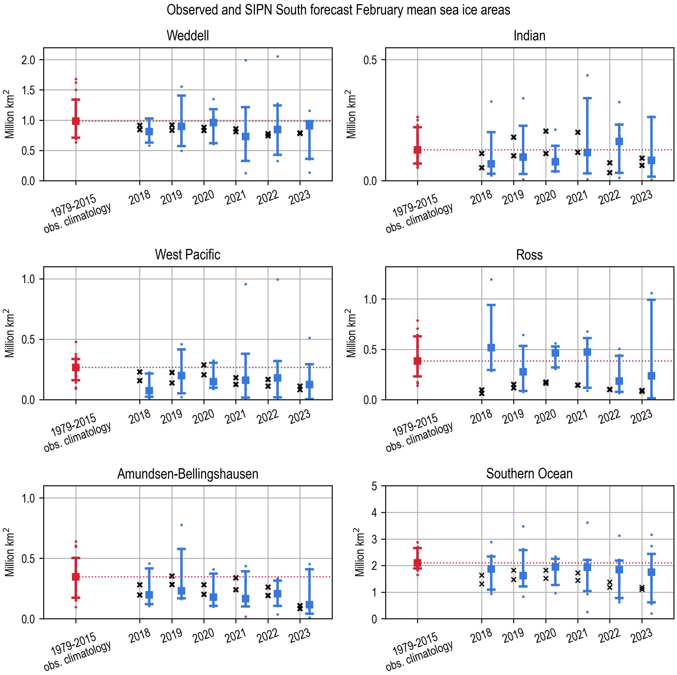
Figure 3 Distribution of the SIPN South forecasts and observed February mean sea ice areas for each of the forecasting seasons. The blue intervals represent the SIPN South distribution (10-90%), with the blue square referring to the ensemble median. The blue dots are those forecasts falling outside the 10-90% bulk of the distribution. The two black crosses denote the observational references. The red interval, square, and dots are the corresponding estimates for the climatological forecast. The light horizontal dotted line is drawn from the median to facilitate the comparison between the forecasts and the climatological state.

The first result is that observational uncertainty (indicated by the difference between the pair of black dots in Figure 3) is generally small in comparison to forecast uncertainty, apart from the Indian Sector, where it can be comparable to the 10-90% forecast range, as in 2020. The Indian Sector is, however, the region with the smallest climatological sea ice area (~5% of the circumpolar area). In absolute value, the observational spread is comparable to the observational spread in other sectors (~0.1 million km² maximum), but the apparent spread is magnified by the fact that the amount of sea ice to predict is very limited.

A second result is that the circumpolar SIPN South range of sea ice areas bracket observations for all years (Figure 3). The SIPN South forecast ensemble is therefore not incompatible, in a statistical sense, with the observations for the total sea ice area. Interestingly, for each year, the medians lie below the 1979-2015 climatological median (horizontal dashed line), suggesting that as a group, the SIPN South forecasts capture well the tendency since 2015 of sea ice area to lie on the low side of the climatological distribution. This gives credit to the SIPN South forecast ensemble having added value over a trivial climatological forecast. We note finally that the historical climatological distribution would be a poor forecast given that all six recently observed states lie below the 10th climatological percentile.

Analyzing regional forecasts allows us to establish whether the total circumpolar sea ice area forecast skill is obtained for the right reasons or thanks to error compensations at the regional scale. The SIPN South forecasts perform generally well in the Weddell Sea, in the West Pacific, and in the Amundsen-Bellingshausen Seas sectors: in those regions, the two observational datasets fall within the forecast range. We have deliberately not reported skill statistics as the sample size (n = 6 years) is very low. The Ross Sea stands out as the region with large systematic errors. The median systematically overestimates the observed values and the observations lie at the edge, if not outside, of the 10-90% forecast range, for reasons that we will discuss in the next section.

Since Figure 3 displays February means, it does not convey information about how the sea ice area was forecast between initialization time (1st of December) and the target month of February. Figure 4 shows the daily evolution of the circumpolar sea ice area (forecast and observed) for the 2022-2023 exercise, for the subset of statistical and dynamical contributions. A striking pattern, also seen for all five previous forecasting seasons (see Supplementary Material), is clear: on average, the SIPN ensemble starts biased high for the circumpolar area; then, from mid-December to mid-January, melt rates are largely overestimated compared to observational references (Figure 4, right column). This feature is particularly evident for dynamical model contributions but is also shared by one statistical contribution.

FIGURE 4

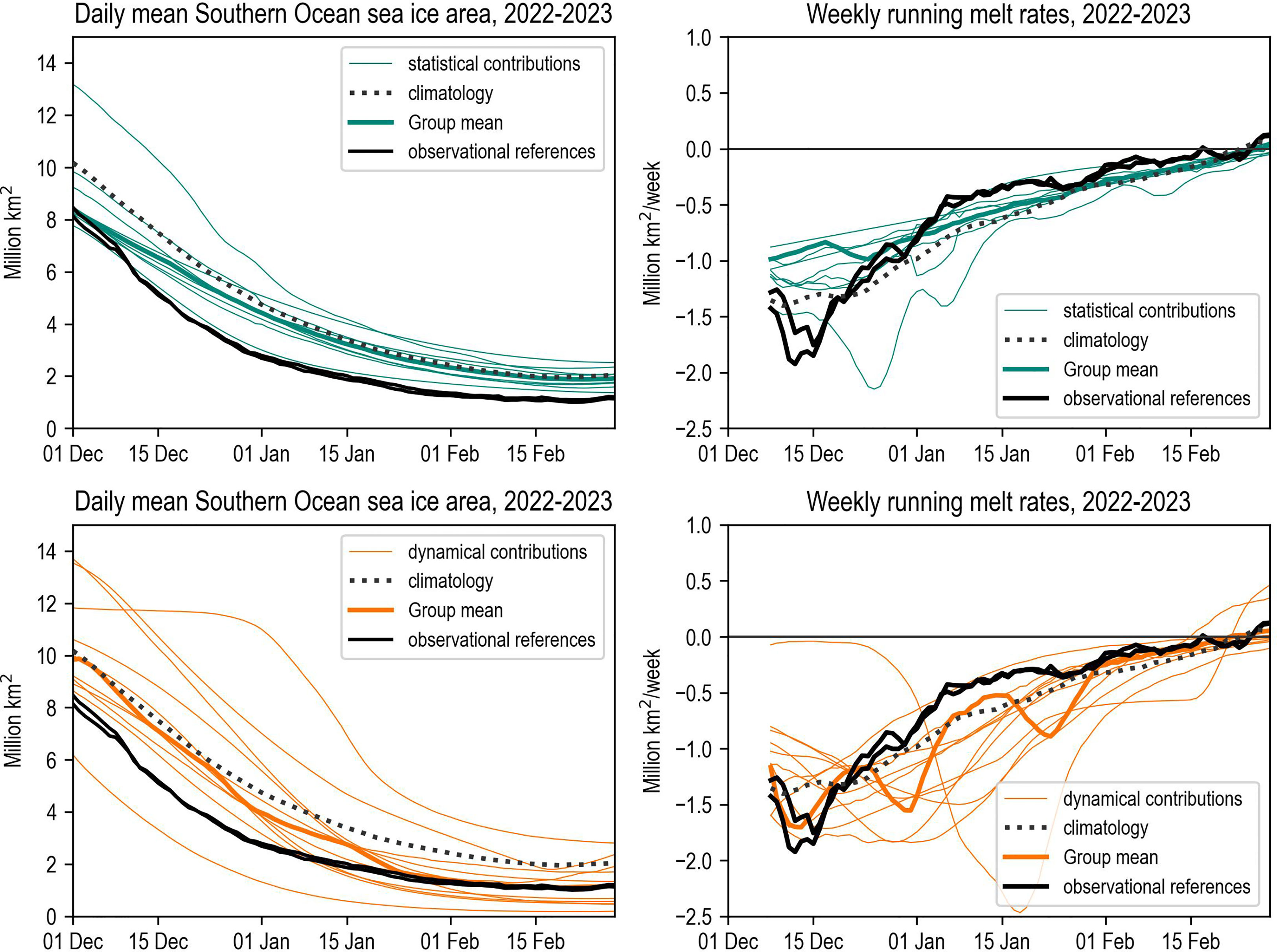
Figure 4 (Left column) Daily Antarctic sea ice area forecast by the groups participating in the 2022-2023 exercise, separated in (top) statistical contributions and (bottom) dynamical contributions. When several ensemble members are submitted by a group, the mean of the distribution is considered. The verifying observational references are shown as thick black lines. The climatological forecast is shown as the black dotted line. (Right column) Running weekly melt rates, computed for day d as the value of the timeseries of the left panel at day d minus the value at day d − 7. The same figures for previous years are shown in the Supplementary Material.

In dynamical model contributions, several reasons can explain this general overestimation of sea ice area at initial time: issues in the initialization procedure or biases in the winter mean state. Regarding the initialization procedure, at least one group (Met Office) follows a “lagged” approach meaning that the ensemble of initial conditions is drawn from the 21 previous days’ (twice a day) states before the initialization date (1st of December). Due to the seasonality of the sea ice area, all corresponding 42 states display a larger sea ice area than the one on Dec 1. For other contributions (e.g., ucl), the source of the problem is different. The ocean–sea ice model exhibits a well-known positive late winter bias in sea ice area (Barthélemy et al., 2018; Massonnet et al., 2019) causing excessive melt rates during the spring season. The origins of this winter bias have not been identified yet but appear to be common to other dynamical models. In statistical contributions, the initial overestimation is less evident: the forecasts appear to be more clustered around the observed state at initial time. An interesting feature is that the climatological forecast itself is biased high on December 1st, consistently with the recent negative anomalies displayed in Figure 1.

3.2 Do SIPN South forecasts provide added value over climatological benchmarks?

With only six seasons of forecasts (2017-2018 to 2022-2023), delivering firm statements on the ability of forecasts to predict interannual variations in sea ice area skill is beyond reach. However, most contributions consist of ensembles of forecasts, so a few conclusions can at least be drawn on the appropriate dispersion properties of individual submissions. To exemplify several aspects of forecast characteristics, we show in Figure 5 the fitted probability density functions of the February mean sea ice area for all groups that participated in the 2022-2023 forecasting season as well as for the climatological forecast. We first note that, in general, statistical model contributions provide fewer ensemble members than dynamical model contributions. A possible reason is that delivering ensemble forecasts has long been standard practice in the weather and climate prediction communities, which frequently construct ensembles to produce probabilistic assessments. Statistical approaches are based on simpler models where it is not always clear how uncertainty should be sampled. All members (colored crosses) in Figure 5 should be viewed as equally plausible forecasts within each submission, except for the NicoSun contribution where each member corresponds to three scenarios of high melt, medium melt, and low melt, respectively.

FIGURE 5

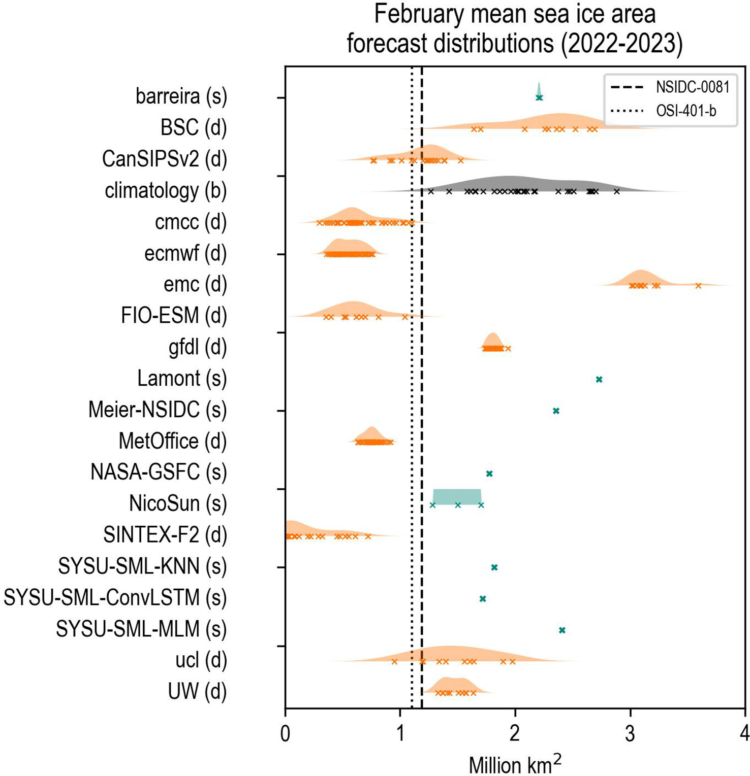
Figure 5 Distribution of the February mean circumpolar sea ice areas forecast by the groups participating in the 2022-2023 season and the verifying observations (vertical dashed lines). The color coding follows the same conventions as in Figure 4. The probability density functions are drawn with a kernel-density estimate using Gaussian kernels.

The first feature that is apparent from Figure 5 is the large variability in the shapes of the forecast distributions. Several contributions are underdispersive (or overconfident) in the sense that the observed value is statistically incompatible with the forecast distribution (e.g., barreira, gfdl). The lack of bias correction is one plausible reason for this behavior. Other contributions are overdispersive (or underconfident) in the sense that the forecast distribution is much wider than the climatology (e.g., SINTEX-F2). Neither underdispersive nor overdispersive ensemble forecasts are desirable from a decision-making point of view: underdispersive forecasts are sharp but most often do not include the actual outcome, while overdispersive forecast distributions most often include the actual outcome but are overly flat.

Striking a good balance between bias (i.e., how far the forecast mean is compared to the verification value) and spread (i.e., how uncertain is the forecast) is essential in ensemble forecasting. The ability to reach a good tradeoff can be measured with a single metric, namely the continuous rank probability (CRPS). The CRPS is a generalization of the Brier Score to continuous variables (Jolliffe and Stephenson, 2003) and measures the area under the squared difference between the cumulative density function of the forecast distribution and the cumulative density function of the observations, i.e., a step function at the observed value. The CRPS is a convenient metric because it penalizes forecasts that are systematically biased high or low, but also forecasts that are excessively spread out. According to the definition, a CRPS value of zero is obtained for a perfect forecast with the mass of the distribution centered at the verifying observation value, and larger CRPS values correspond to less skillful forecasts.

The CRPS values for all six forecasting seasons are reported in Table 2. Caution should be exercised when interpreting the results in this table since the CRPS, like any metric of performance, is sensitive to sampling issues. Nevertheless, several interesting features are noted. First, no obvious relationship emerges between the type of forecasting approach and the CRPS metric: the statistical and dynamical sub-groups score an average value of 0.57 and 0.49 million km² squared for the six forecasting seasons, respectively. Second, we note that 51% (42 out of 82) predictions are superior, in a CRPS sense, to the climatological forecast. This proportion raises to 65% (22 out of 34) for the last two seasons when an all-time minimum occurred (2021-2022 and then 2022-2023). Several individual contributions systematically outperform that benchmark forecast. Finally, the group forecast, obtained by aggregating individual forecasts (see Sec. 2.3) is systematically more skilled than the climatological forecast and more skilled than most of the individual forecasts. We also note that the CRPS of the statistical and dynamical sub-group forecast is more skilled than the average CRPS within each respective group. This behavior is reminiscent of what is observed with the multi-model mean in climate change simulations, and is likely explained by the cancellation of random errors that characterize individual forecasts.

TABLE 2

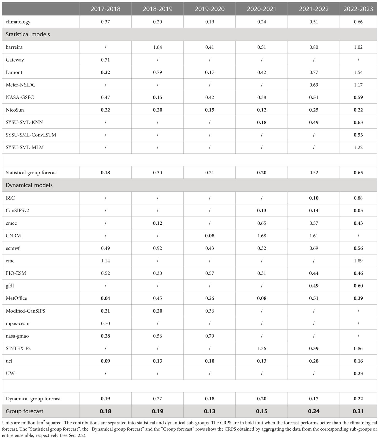
Table 2 Continuous Rank Probability Scores (CRPS) for the February mean Antarctic sea ice area forecasts, for each of the forecasting seasons of the SIPN South project.

3.3 Is there a relationship between forecasting approach and skill?

The previous section has hinted at the fact that, from a circumpolar point of view, no sub-group of forecasts (statistical or dynamical) outperforms the other. The results have also suggested the value of aggregating the individual forecasts to produce a group forecast. On the other hand, Section 3.1 has shown that the skill is region-dependent in the SIPN South ensemble. To assess the ability of the prediction systems to capture the regional distribution of sea ice concentration, we compute the Integrated Ice Edge Error (IIEE, Goessling et al. (2016)). The IIEE is the areal integral of all grid cells where the forecast and the verification disagree on a certain event, defined here as sea ice presence (SIC > 15%). For one-member forecasts, the calculation of the IIEE is straightforward: the spatial fields of SIC are converted to 1 or 0 based on the 15% SIC threshold and the resulting binary field is compared to the observed binary field of ice presence. The areas of grid cells where sea ice is present in observations but absent in the forecasts, or absent in observations but present in the forecasts are then summed. For multi-member forecasts, the calculation is slightly different: binary fields of sea ice presence are defined for each member individually, and a probability of sea ice presence is calculated by averaging the binary fields across the ensemble. The areas of grid cells where sea ice present in observations but present with < 50% probability in the ensemble, or absent in observations but present with > 50% in the ensemble, are then summed. To compute the IIEE, all forecasts and verification data were first remapped (nearest-neighbor interpolation) to a 2° by 2° regular grid.

The IIEEs for the 2022-2023 forecasting season are shown in Figure 6. In line with Figure 4 (circumpolar sea ice area daily time series), dynamical predictions in general exhibit larger initial errors than statistical predictions. These initial errors in dynamical predictions develop throughout the melting season until ~1st of January, before a sharp reduction towards the month of February. For that month, no type of prediction appears to be superior to another for the IIEE metric. The group forecast has an IIEE that is among the lowest from early February, confirming at the regional scale the conclusions obtained at the circumpolar scale.

FIGURE 6

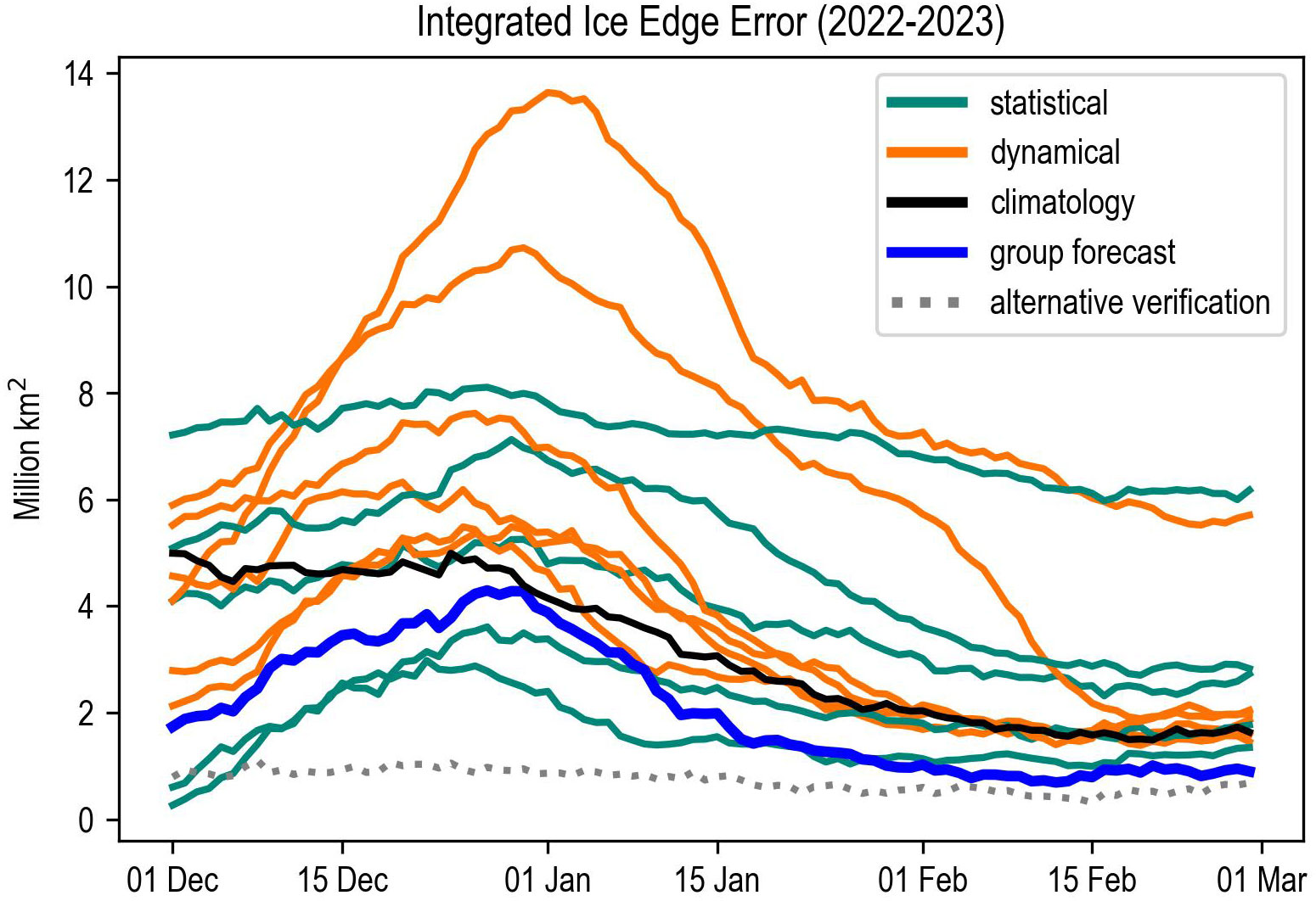
Figure 6 Integrated Ice Edge Error (see the text for definition) for the contributions providing the sea ice concentration information. The color coding follows the same conventions as in Figure 4. The black curve is the benchmark climatological forecast (see Section 2.4) and the thick blue curve is the IIEE of the group forecast. The reference product for the IIEE calculation is the NSIDC-0081 product, and the grey curve shows the IIEE of the alternative verification product OSI-401-b.

4 Conclusions, perspectives, and recommendations

The SIPN South project was initiated in 2017, i.e., one year after the beginning of a series of anomalously low sea ice conditions in the Southern Ocean (Figure 1). The non-stationary character of sea ice area anomalies suggests that climatological forecasts could be of limited value for seasonal prediction. An important finding of this study is that several prediction systems, based on both statistical and dynamical modeling, are consistently more skillful than the climatological forecast. The group forecast, obtained by aggregating all individual forecasts, is found to outperform the climatological forecast and the majority of individual forecasts themselves for two standard metrics of performance, the continuous rank probability score and the integrated ice edge error.

The Ross Sea appears to be the sector where sea ice prediction is the most challenging and where spread is the largest, although a recent study (Payne et al., 2022) demonstrates moderate skill in the sector with a dynamical model. While we have not attempted here to understand the sources of prediction errors and why they vary regionally, we can formulate hypotheses. The Ross Sea summer sea ice concentration anomalies are linked to the spring sea ice drift and thickness anomalies in the neighboring Amundsen Sea sector. In observations, westward coastal currents transport sea ice toward the Ross ice shelf during the spring season, and sea ice is then advected offshore by the dominant southerly winds (e.g., Holland and Kimura, 2016). This coupled dynamical process is difficult to simulate at the resolution of current ocean-sea ice dynamical models (Holland et al., 2014). In addition, the statistical models participating in SIPN South (Table 1) do not consider the initial sea ice thickness as a predictor except for one (NicoSun), which turns out to be performing relatively well. The poor performance of forecasts in the Ross Sea could also be explained by the fact that predictability is inherently lower there compared to other sectors. In dynamical model predictions, ensemble spread is usually the largest in the Ross sea (not shown), which supports this idea of limited initial-value predictability in that sector.

Several studies have reported long-range (>1 yr) sea ice predictability thanks to mechanisms of reemergence (e.g., Holland et al., 2013; Marchi et al., 2019) and the results of SIPN South might appear disappointing, at least in light of the initial prospects raised in these perfect predictability studies. The ocean-to-sea ice connection that brings the long-range predictability of surface conditions is more direct in winter (since the deep mixing causes direct interaction), whereas the summer connection requires simulation of more complex process (mixed layer shoaling, ice-albedo feedback, vertical mixing, etc.), which is likely not captured by the current models.

The results of this study have highlighted that dynamical models, even when they are initialized with observed or reanalyzed ocean-sea ice states, exhibit a positive bias in sea ice area at initial time but no bias at the sea ice minimum, implying excessive sea ice area losses during the melting season. The reason could be that the dynamical contributions are initialized with different products from the ones used for verification. More diagnostics (e.g., tendencies in sea ice concentration due to thermodynamic and dynamic processes) would be required to pinpoint the deficient physical mechanisms in these models.

For the metrics of performance introduced in this paper, the statistical models appear to perform better than the dynamical models for predicting the spatial information during the melting season (December and January, see the IIEE curves in Figure 6). Nonetheless, a limitation of statistical contributions is that most of them are deterministic, i.e., provide only one prediction (the NicoSun is an exception, providing forecasts as a range of three scenarios: low melt, medium melt, high melt). The deterministic nature of most statistical forecasts is contrasted by the large ensemble size in dynamical models, exceeding 50 ensemble members for several dynamical contributions, and can be regarded as a serious limitation to the use of these statistical predictions by stakeholders. Stakeholder-relevant diagnostics like the probability of sea-ice presence (i.e., the probability of observing sea ice concentration above 15% at a given point at a given day) cannot be reliably estimated with statistical models alone when they provide only one or even three ensemble members. In this context it is worth mentioning that one of the statistical SIPN South contributions, AWI-SDAP, provided just that probability of sea ice presence instead of sea ice concentration (although only for one year). However, this contribution could not be included in all analyses because it is not possible to derive sea-ice area from the probability of ice presence. In future intercomparison studies, we might thus recommend submitting forecasts of the probability of sea ice presence directly.

The conclusions presented here draw on six seasons of coordinated sea ice predictions since 2017. One of the novel aspects of SIPN South is that it collects predictions done in a real-time context with the best possible information available at the time of submission by each group. These predictions differ from hindcasts (retrospective forecasts) that are less constrained by data unavailability (since ocean/atmosphere/sea ice reanalyses are released with a couple of weeks or months of delay). Also, hindcasts might exhibit larger skill than real-time forecasts due to the fact that the models are, consciously or not, continuously adapted and tuned to represent new climatic situations.

The principal value of the SIPN South community effort is to identify and engage contributors on best practices, while exploring the current skill in forecasting austral summer sea ice conditions. We are aware that we might miss potential contributions from individuals, groups, or institutions that are not registered on those lists or on social media. We will continue to regularly collect forecasts for the summer season, and are currently expanding the protocol for other seasons. The possibility to submit more diagnostics such as sea ice drift and thickness, oceanic mixed layer depth and heat content, will be added to the SIPN South protocol to better partition forecast errors between initial-condition uncertainty and model uncertainty. We will also consider developing near-operational benchmark datasets beyond simple climatology. Future work will also include a more systematic evaluation of skill at the regional scale, will accept longer forecasts (out to fall and winter), and will allow contributors to re-submit forecasts in a hindcast context, i.e. when all datasets at initial times are available.

Data availability statement

The datasets presented in this study can be found in online repositories. The names of the repository/repositories and accession number(s) can be found in the article/Supplementary Material.

Author contributions

All co-authors provided the data. FM wrote the manuscript, all co-authors edited and commented it. All authors contributed to the article and approved the submitted version.

Funding

QY, XL and XD are supported by the National Key R&D Program of China (No. 2022YFE0106300) and the National Natural Science Foundation of China (No. 41941009, 42106233). WaM is supported by the NASA Earth Science Data Information System (ESDIS) Project through the NASA Snow and Ice Distributed Active Archive Center (DAAC) at NSIDC. WH is supported by grant funding from the Australian Government as part of the Antarctic Science Collaboration Initiative program. HG and BN acknowledge the financial support by the Federal Ministry of Education and Research of Germany in the framework of SSIP (grant 01LN1701A). EB-W was funded by National Science Foundation grant NSF-RAPID OPP-2233016.

Acknowledgments

FM is a F.R.S.-FNRS Research Associate. EB was supported by the Met Office Hadley Centre Climate Programme funded by BEIS and Defra. XY and CL are supported by Lamont-Dohert Earth Observatory of Columbia University and a private donor (Ying). YM is supported by JSPS KAKENHI Grant Number 22K03727 and Princeton University/NOAA GFDL Visiting Research Scientists Program. SINTEX-F2 seasonal forecast was performed on Earth Simulator at JAMSTEC. AS was supported by Copernicus Climate Change Service (C3S2_370) Operational Seasonal Predictions, DI by the Foundation Euro-Mediterranean Center on Climate Change (CMCC, Italy).

Conflict of interest

The authors declare that the research was conducted in the absence of any commercial or financial relationships that could be construed as a potential conflict of interest.

Publisher’s note

All claims expressed in this article are solely those of the authors and do not necessarily represent those of their affiliated organizations, or those of the publisher, the editors and the reviewers. Any product that may be evaluated in this article, or claim that may be made by its manufacturer, is not guaranteed or endorsed by the publisher.

Supplementary material

The Supplementary Material for this article can be found online at: https://www.frontiersin.org/articles/10.3389/fmars.2023.1148899/full#supplementary-material

References

Abrahamsen E. P., Barreira S., Bitz C. M., Butler A., Clem K. R., Colwell S., et al. (2020). Antarctica And the southern ocean. Bull. Am. Meteorol. Soc. 101 (8), S287−S320. doi: 10.1175/BAMS-D-20-0090.1

CrossRef Full Text | Google Scholar

Barthélemy A., Goosse H., Fichefet T., Lecomte O. (2018). On the sensitivity of Antarctic sea ice model biases to atmospheric forcing uncertainties. Climate Dynamics. 51 (4), 1585−1603. doi: 10.1007/s00382-017-3972-7

CrossRef Full Text | Google Scholar

Bilbao R., Wild S., Ortega P., Acosta-Navarro J., Arsouze T., Bretonnière P.-A., et al. (2021). Assessment of a full-field initialized decadal climate prediction system with the CMIP6 version of EC-earth. Earth Syst. Dynamics. 12 (1), 173−196. doi: 10.5194/esd-12-173-2021

CrossRef Full Text | Google Scholar

Blanchard-Wrigglesworth E., Bushuk M., Massonnet F., Hamilton L. C., Bitz C. M., Meier W. N., et al. (2023). Forecast skill of the Arctic Sea ice outlook 2008–2022. Geophys. Res. Lett. 50 (6), e2022GL102531. doi: 10.1029/2022GL102531

CrossRef Full Text | Google Scholar

Blanchard-Wrigglesworth E., Cullather R. I., Wang W., Zhang J., Bitz C. M. (2015). Model forecast skill and sensitivity to initial conditions in the seasonal Sea ice outlook. Geophys. Res. Lett. 42 (19), 8042−8048. doi: 10.1002/2015GL065860

CrossRef Full Text | Google Scholar

Brierley A. S., Thomas D. N. (2002). Ecology of southern ocean pack ice. Adv. Mar. Biol. 43, 171−276. doi: 10.1016/s0065-2881(02)43005-2

CrossRef Full Text | Google Scholar

Bromwich D. H., Werner K., Casati B., Powers J. G., Gorodetskaya I. V., Massonnet F., et al. (2020). The year of polar prediction in the southern hemisphere (YOPP-SH). Bull. Am. Meteorol. Soc. 101, E1653–E1676. doi: 10.1175/BAMS-D-19-0255.1

CrossRef Full Text | Google Scholar

Bushuk M., Winton M., Haumann F. A., Delworth T., Lu F., Zhang Y., et al. (2021). Seasonal prediction and predictability of regional Antarctic sea ice. J. Climate 1 (aop), 1−68. doi: 10.1175/JCLI-D-20-0965.1

CrossRef Full Text | Google Scholar

Caron L.-P., Massonnet F., Klotzbach P. J., Philp T. J., Stroeve J. (2020). Making seasonal outlooks of Arctic Sea ice and Atlantic hurricanes valuable–not just skillful. Bull. Am. Meteorol. Soc. 101 (1), E36−E42. doi: 10.1175/BAMS-D-18-0314.1

CrossRef Full Text | Google Scholar

Cavalieri D. J., Parkinson C. L., Vinnikov K. Y. (2003). 30-year satellite record reveals contrasting Arctic and Antarctic decadal sea ice variability. Geophys. Res. Lett. 30 (18), 1–4. doi: 10.1029/2003GL018031

CrossRef Full Text | Google Scholar

Chen H., Yin X., Bao Y., Qiao F. (2016). Ocean satellite data assimilation experiments in FIO-ESM using ensemble adjustment kalman filter. Sci. China Earth Sci. 59 (3), 484−494. doi: 10.1007/s11430-015-5187-2

CrossRef Full Text | Google Scholar

Chen D., Yuan X. (2004). A Markov model for seasonal forecast of Antarctic Sea ice. J. Climate 17, 13. doi: 10.1175/1520-0442(2004)017<3156:AMMFSF>2.0.CO;2

CrossRef Full Text | Google Scholar

Cherchi A., Fogli P. G., Lovato T., Peano D., Iovino D., Gualdi S., et al. (2019). Global mean climate and main patterns of variability in the CMCC-CM2 coupled model. J. Adv. Modeling. Earth Syst. 11 (1), 185−209. doi: 10.1029/2018MS001369

CrossRef Full Text | Google Scholar

Chevallier M., Massonnet F., Goessling H., Guémas V., Jung T. (2019). Sub-Seasonal. to Seasonal. Prediction., 201−221. doi: 10.1016/B978-0-12-811714-9.00010-3

CrossRef Full Text | Google Scholar

COMNAP (2015) COMNAP sea ice challenges workshop report : Hobart, Tasmania, Australia, 12-13 may 2015. Available at: https://static1.squarespace.com/static/61073506e9b0073c7eaaf464/t/615a56981ab568669d8e4554/1633310364849/COMNAP_Sea_Ice_Challenges_BKLT_Web_Final_Dec2015.pdf.

Google Scholar

Delille B., Vancoppenolle M., Geilfus N.-X., Tilbrook B., Lannuzel D., Schoemann V., et al. (2014). Southern ocean CO2 sink : the contribution of the sea ice. J. Geophys. Res.: Oceans. 119 (9), 6340−6355. doi: 10.1002/2014JC009941

CrossRef Full Text | Google Scholar

Delworth T. L., Cooke W. F., Adcroft A., Bushuk M., Chen J., Dunne K. A., et al. (2020). SPEAR : the next generation GFDL modeling system for seasonal to multidecadal prediction and projection. J. Adv. Modeling. Earth Syst. 12 (3). doi: 10.1029/2019MS001895

CrossRef Full Text | Google Scholar

DeVries T. (2014). The oceanic anthropogenic CO2 sink : storage, air-sea fluxes, and transports over the industrial era. Global Biogeochem. Cycles. 28 (7), 631−647. doi: 10.1002/2013GB004739

CrossRef Full Text | Google Scholar

Dirkson A., Merryfield W. J., Monahan A. (2017). Impacts of Sea ice thickness initialization on seasonal Arctic Sea ice predictions. J. Climate 30 (3), 1001−1017. doi: 10.1175/JCLI-D-16-0437.1

CrossRef Full Text | Google Scholar

Doi T., Behera S. K., Yamagata T. (2016). Improved seasonal prediction using the SINTEX-F2 coupled model. J. Adv. Modeling. Earth Syst. 8 (4), 1847−1867. doi: 10.1002/2016MS000744

CrossRef Full Text | Google Scholar

Donlon C. J., Martin M., Stark J., Roberts-Jones J., Fiedler E., Wimmer W. (2012). The operational Sea surface temperature and Sea ice analysis (OSTIA) system. Remote Sens. Environ. 116, 140−158. doi: 10.1016/j.rse.2010.10.017

CrossRef Full Text | Google Scholar

Eayrs C., Li X., Raphael M. N., Holland D. M. (2021). Rapid decline in Antarctic sea ice in recent years hints at future change. Nat. Geosci. 14, 1−5. doi: 10.1038/s41561-021-00768-3

CrossRef Full Text | Google Scholar

Ferro C. A. T. (2017). Measuring forecast performance in the presence of observation error : measuring forecast performance in the presence of observation error. Q. J. R. Meteorol. Soc. 143 (708), 2665−2676. doi: 10.1002/qj.3115

CrossRef Full Text | Google Scholar

Gelaro R., McCarty W., Suárez M. J., Todling R., Molod A., Takacs L., et al. (2017). The modern-era retrospective analysis for research and applications, version 2 (MERRA-2). J. Climate 30 (14), 5419−5454. doi: 10.1175/JCLI-D-16-0758.1

CrossRef Full Text | Google Scholar

Goessling H. F., Tietsche S., Day J. J., Hawkins E., Jung T. (2016). Predictability of the Arctic sea ice edge. Geophys. Res. Lett. 43 (4), 1642−1650. doi: 10.1002/2015GL067232

CrossRef Full Text | Google Scholar

Goosse H., Kay J. E., Armour K. C., Bodas-Salcedo A., Chepfer H., Docquier D., et al. (2018). Quantifying climate feedbacks in polar regions. Nat. Commun. 9 (1), 1−13. doi: 10.1038/s41467-018-04173-0

PubMed Abstract | CrossRef Full Text | Google Scholar

Goosse H., Zunz V. (2014). Decadal trends in the Antarctic sea ice extent ultimately controlled by ice–ocean feedback. Cryosphere. 8 (2), 453−470. doi: 10.5194/tc-8-453-2014

CrossRef Full Text | Google Scholar

Gray A. R., Johnson K. S., Bushinsky S. M., Riser S. C., Russell J. L., Talley L. D., et al. (2018). Autonomous biogeochemical floats detect significant carbon dioxide outgassing in the high-latitude southern ocean. Geophys. Res. Lett. 45 (17), 9049−9057. doi: 10.1029/2018GL078013

CrossRef Full Text | Google Scholar

Griffies S. M. (2012). Elements of the modular ocean model. GFDL ocean group technical report no. 7 (Princeton: NOAA/Geophysical Fluid Dynamics Laboratory), 632.

Google Scholar

Hamilton L. C., Stroeve J. (2016). 400 predictions : the SEARCH Sea ice outlook 2008–2015. Polar. Geogr. 39 (4), 274−287. doi: 10.1080/1088937X.2016.1234518

CrossRef Full Text | Google Scholar

Hobbs W. R., Massom R., Stammerjohn S., Reid P., Williams G., Meier W. (2016). A review of recent changes in southern ocean sea ice, their drivers and forcings. Global Planet. Change 143, 228−250. doi: 10.1016/j.gloplacha.2016.06.008

CrossRef Full Text | Google Scholar

Holland M. M., Blanchard-Wrigglesworth E., Kay J., Vavrus S. (2013). Initial-value predictability of Antarctic sea ice in the community climate system model 3. Geophys. Res. Lett. 40 (10), 2121−2124. doi: 10.1002/grl.50410

CrossRef Full Text | Google Scholar

Holland P. R., Bruneau N., Enright C., Losch M., Kurtz N. T., Kwok R. (2014). Modeled trends in Antarctic Sea ice thickness. J. Climate 27 (10), 3784−3801. doi: 10.1175/JCLI-D-13-00301.1

CrossRef Full Text | Google Scholar

Holland P. R., Kimura N. (2016). Observed concentration budgets of Arctic and Antarctic Sea ice. J. Climate 29 (14), 5241−5249. doi: 10.1175/JCLI-D-16-0121.1

CrossRef Full Text | Google Scholar

Holland M. M., Landrum L., Raphael M., Stammerjohn S. (2017). Springtime winds drive Ross Sea ice variability and change in the following autumn. Nat. Commun. 8 (1), 731. doi: 10.1038/s41467-017-00820-0

PubMed Abstract | CrossRef Full Text | Google Scholar

Hunke E. C., Lipscomb W. H. (2010). CICE: the Los alamos sea ice model documentation and software user’s manual (Los Alamos: T-3 Fluid Dynamics Group, Los Alamos National Laboratory), 76.

Google Scholar

Johnson S. J., Stockdale T. N., Ferranti L., Balmaseda M. A., Molteni F., Magnusson L., et al. (2019). SEAS5 : the new ECMWF seasonal forecast system. Geosci. Model. Dev. 12 (3), 1087−1117. doi: 10.5194/gmd-12-1087-2019

CrossRef Full Text | Google Scholar

Jolliffe I. T., Stephenson ,. D. B. (Eds.) (2003). Forecast verification : a practitioner’s guide in atmospheric science (Chichester, West Sussex, England and Hoboken, NJ: J. Wiley).

Google Scholar

Jung T., Gordon N. D., Bauer P., Bromwich D. H., Chevallier M., Day J. J., et al. (2016). Advancing polar prediction capabilities on daily to seasonal time scales. Bull. Am. Meteorol. Soc. 97 (9), 1631−1647. doi: 10.1175/BAMS-D-14-00246.1

CrossRef Full Text | Google Scholar

Kohout A. L., Williams M. J. M., Dean S. M., Meylan M. H. (2014). Storm-induced sea-ice breakup and the implications for ice extent. Nature 509 (7502), 604−607. doi: 10.1038/nature13262

CrossRef Full Text | Google Scholar

Koster R. D., Suarez M. J., Ducharne A., Stieglitz M., Kumar P. (2000). A catchment-based approach to modeling land surface processes in a general circulation model : 1. model structure. J. Geophys. Res.: Atmospheres. 105 (D20), 24809−24822. doi: 10.1029/2000JD900327

CrossRef Full Text | Google Scholar

Lavergne T., Sørensen A. M., Kern S., Tonboe R., Notz D., Aaboe S., et al. (2019). Version 2 of the EUMETSAT OSI SAF and ESA CCI sea-ice concentration climate data records. Cryosphere. 13 (1), 49−78. doi: 10.5194/tc-13-49-2019

CrossRef Full Text | Google Scholar

Libera S., Hobbs W., Klocker A., Meyer A., Matear R. (2022). Ocean-Sea ice processes and their role in multi-month predictability of Antarctic Sea ice. Geophys. Res. Lett. 49 (8), e2021GL097047. doi: 10.1029/2021GL097047

CrossRef Full Text | Google Scholar

Lin X., Massonnet F., Fichefet T., Vancoppenolle M. (2021). SITool (v1.0) – a new evaluation tool for large-scale sea ice simulations : application to CMIP6 OMIP. Geosci. Model. Dev. 14 (10), 6331−6354. doi: 10.5194/gmd-14-6331-2021

CrossRef Full Text | Google Scholar

Lin H., Merryfield W. J., Muncaster R., Smith G. C., Markovic M., Dupont F., et al. (2020). The Canadian seasonal to interannual prediction system version 2 (CanSIPSv2). Weather. Forecasting. 35 (4), 1317−1343. doi: 10.1175/WAF-D-19-0259.1

CrossRef Full Text | Google Scholar

Liu H., Yu W., Chen X. (2022). Melting Antarctic Sea ice is yielding adverse effects on a short-lived squid species in the Antarctic adjacent waters. Front. Mar. Sci. 9. doi: 10.3389/fmars.2022.819734

PubMed Abstract | CrossRef Full Text | Google Scholar

Liu J., Zhu Z., Chen D. (2023). Lowest Antarctic sea ice record broken for the second year in a row. Ocean-Land-Atmosphere. Res. 0 (ja). doi: 10.34133/olar.0007

CrossRef Full Text | Google Scholar

Lu F., Harrison M. J., Rosati A., Delworth T. L., Yang X., Cooke W. F., et al. (2020). GFDL’s SPEAR seasonal prediction System : initialization and ocean tendency adjustment (OTA) for coupled model predictions. J. Adv. Modeling. Earth Syst. 12 (12), e2020MS002149. doi: 10.1029/2020MS002149

CrossRef Full Text | Google Scholar

MacLachlan C., Arribas A., Peterson K. A., Maidens A., Fereday D., Scaife A. A., et al. (2015). Global seasonal forecast system version 5 (GloSea5) : a high-resolution seasonal forecast system. Q. J. R. Meteorol. Soc. 141 (689), 1072−1084. doi: 10.1002/qj.2396

CrossRef Full Text | Google Scholar

Marchi S., Fichefet T., Goosse H., Zunz V., Tietsche S., Day J. J., et al. (2019). Reemergence of Antarctic sea ice predictability and its link to deep ocean mixing in global climate models. Climate Dynamics. 52 (5−6), 2775−2797. doi: 10.1007/s00382-018-4292-2

CrossRef Full Text | Google Scholar

Martinson D. G. (1990). Evolution of the southern ocean winter mixed layer and sea ice : open ocean deepwater formation and ventilation. J. Geophys. Res. 95 (C7), 11641. doi: 10.1029/JC095iC07p11641

CrossRef Full Text | Google Scholar

Massom R. A., Scambos T. A., Bennetts L. G., Reid P., Squire V. A., Stammerjohn S. E. (2018). Antarctic Ice shelf disintegration triggered by sea ice loss and ocean swell. Nature 558 (7710), 383−389. doi: 10.1038/s41586-018-0212-1

CrossRef Full Text | Google Scholar

Massonnet F., Barthélemy A., Worou K., Fichefet T., Vancoppenolle M., Rousset C., et al. (2019). On the discretization of the ice thickness distribution in the NEMO3.6-LIM3 global ocean–sea ice model. Geosci. Model. Dev. 12 (8), 3745−3758. doi: 10.5194/gmd-12-3745-2019

CrossRef Full Text | Google Scholar

Massonnet F., Bellprat O., Guemas V., Doblas-Reyes F. J. (2016). Using climate models to estimate the quality of global observational data sets. Science 354 (6311), 452−455. doi: 10.1126/science.aaf6369

CrossRef Full Text | Google Scholar

Massonnet F., Mathiot P., Fichefet T., Goosse H., König Beatty C., Vancoppenolle M., et al. (2013). A model reconstruction of the Antarctic sea ice thickness and volume changes over 1980–2008 using data assimilation. Ocean. Model. 64, 67−75. doi: 10.1016/j.ocemod.2013.01.003

CrossRef Full Text | Google Scholar

Meehl G. A., Arblaster J. M., Chung C. T. Y., Holland M. M., DuVivier A., Thompson L., et al. (2019). Sustained ocean changes contributed to sudden Antarctic sea ice retreat in late 2016. Nat. Commun. 10 (1), 14. doi: 10.1038/s41467-018-07865-9

PubMed Abstract | CrossRef Full Text | Google Scholar

Meier W., Stewart J. S., Wilcox H., Hardman M. A., Scott D. J. (2022) Near-Real-Time DMSP SSMIS daily polar gridded Sea ice concentrations, version 2. Available at: https://nsidc.org/data/nsidc-0081.

Google Scholar

Merryfield W. J., Lee W.-S., Boer G. J., Kharin V. V., Scinocca J. F., Flato G. M., et al. (2013). The Canadian seasonal to interannual prediction system. part I : models and initialization. Monthly. Weather. Rev. 141 (8), 2910−2945. doi: 10.1175/MWR-D-12-00216.1

CrossRef Full Text | Google Scholar

Molod A., Takacs L., Suarez M., Bacmeister J. (2015). Development of the GEOS-5 atmospheric general circulation model : evolution from MERRA to MERRA2. Geosci. Model. Dev. 8 (5), 1339−1356. doi: 10.5194/gmd-8-1339-2015

CrossRef Full Text | Google Scholar

Morioka Y., Doi T., Iovino D., Masina S., Behera S. K. (2019). Role of sea-ice initialization in climate predictability over the weddell Sea. Sci. Rep. 9 (1), 2457. doi: 10.1038/s41598-019-39421-w

PubMed Abstract | CrossRef Full Text | Google Scholar

Morioka Y., Iovino D., Cipollone A., Masina S., Behera S. K. (2021). Summertime sea-ice prediction in the weddell Sea improved by sea-ice thickness initialization. Sci. Rep. 11 (1), 11475. doi: 10.1038/s41598-021-91042-4

PubMed Abstract | CrossRef Full Text | Google Scholar

Mortimer C., Mudryk L., Derksen C., Luojus K., Brown R., Kelly R., et al. (2020). Evaluation of long-term northern hemisphere snow water equivalent products. Cryosphere. 14 (5), 1579−1594. doi: 10.5194/tc-14-1579-2020

CrossRef Full Text | Google Scholar

Niraula B., Goessling H. F. (2021). Spatial damped anomaly persistence of the Sea ice edge as a benchmark for dynamical forecast systems. J. Geophys. Res.: Oceans. 126 (12), e2021JC017784. doi: 10.1029/2021JC017784

CrossRef Full Text | Google Scholar

Ordoñez A. C., Bitz C. M., Blanchard-Wrigglesworth E. (2018). Processes controlling Arctic and Antarctic Sea ice predictability in the community earth system model. J. Climate 31 (23), 9771−9786. doi: 10.1175/JCLI-D-18-0348.1

CrossRef Full Text | Google Scholar

Parkinson C. L. (2019). A 40-y record reveals gradual Antarctic sea ice increases followed by decreases at rates far exceeding the rates seen in the Arctic. Proc. Natl. Acad. Sci. 116 (29), 14414−14423. doi: 10.1073/pnas.1906556116

CrossRef Full Text | Google Scholar

Payne G., Martin J., Monahan A., Sigmond M. (2022). Seasonal predictions of regional and pan-Antarctic sea ice with a dynamical forecast system. (Victoria, British Columbia, Canada).

Google Scholar

Petty A. A., Schröder D., Stroeve J. C., Markus T., Miller J., Kurtz N. T., et al. (2017). Skillful spring forecasts of September Arctic sea ice extent using passive microwave sea ice observations. Earth’s. Future 5 (2), 254−263. doi: 10.1002/2016EF000495

CrossRef Full Text | Google Scholar

Purich A., England M. H. (2019). Tropical teleconnections to Antarctic Sea ice during austral spring 2016 in coupled pacemaker experiments. Geophys. Res. Lett. 46 (12), 6848−6858. doi: 10.1029/2019GL082671

CrossRef Full Text | Google Scholar

Qiao F., Song Z., Bao Y., Song Y., Shu Q., Huang C., et al. (2013). Development and evaluation of an earth system model with surface gravity waves. J. Geophys. Res.: Oceans. 118 (9), 4514−4524. doi: 10.1002/jgrc.20327

CrossRef Full Text | Google Scholar

Raphael M. N., Handcock M. S. (2022). A new record minimum for Antarctic sea ice. Nat. Rev. Earth Environ. 3, 1−2. doi: 10.1038/s43017-022-00281-0

CrossRef Full Text | Google Scholar

Rienecker M. (2008). GEOS-5 data assimilation system–documentation of versions 5.0.1, 5.1.0, and 5.2.0. technical report series on global modeling and data assimilation, NASA/TM–2008–104606, Vol. 27. 1–118.

Google Scholar

Roach L. A., Dörr J., Holmes C. R., Massonnet F., Blockley E. W., Notz D., et al. (2020). Antarctic Sea Ice area in CMIP6. Geophys. Res. Lett. 47 (9). doi: 10.1029/2019GL086729

CrossRef Full Text | Google Scholar

Saha S., Moorthi S., Wu X., Wang J., Nadiga S., Tripp P., et al. (2014). The NCEP climate forecast system version 2. J. Climate 27 (6), 2185−2208. doi: 10.1175/JCLI-D-12-00823.1

CrossRef Full Text | Google Scholar

Schlosser E., Haumann F. A., Raphael M. N. (2018). Atmospheric influences on the anomalous 2016 Antarctic sea ice decay. Cryosphere. 12 (3), 1103−1119. doi: 10.5194/tc-12-1103-2018

CrossRef Full Text | Google Scholar

Shi X., Chen Z., Wang H., Yeung D.-Y., Wong W., WOO W. (2015). Convolutional LSTM Network : a machine learning approach for precipitation nowcasting. Adv. Neural Inf. Process. Syst. 28.

Google Scholar

Steele M., Eicken H., Bhatt U., Bieniek P., Blanchard-Wrigglesworth E., Wiggins H., et al. (2021). Moving Sea ice prediction forward Via community intercomparison. Bull. Am. Meteorol. Soc. 1 (aop), 1−7. doi: 10.1175/BAMS-D-21-0159.1

CrossRef Full Text | Google Scholar

Stuecker M. F., Bitz C. M., Armour K. C. (2017). Conditions leading to the unprecedented low Antarctic sea ice extent during the 2016 austral spring season. Geophys. Res. Lett. 44 (17), 9008−9019. doi: 10.1002/2017GL074691

CrossRef Full Text | Google Scholar

Tebaldi C., Knutti R. (2007). The use of the multi-model ensemble in probabilistic climate projections. Philos. Trans. R. Soc. A: Mathematical. Phys. Eng. Sci. 365 (1857), 2053−2075. doi: 10.1098/rsta.2007.2076

CrossRef Full Text | Google Scholar

Tejedo P., Benayas J., Cajiao D., Leung Y.-F., De Filippo D., Liggett D. (2022). What are the real environmental impacts of Antarctic tourism? unveiling their importance through a comprehensive meta-analysis. J. Environ. Manage. 308, 114634. doi: 10.1016/j.jenvman.2022.114634

PubMed Abstract | CrossRef Full Text | Google Scholar

Tonboe R., Lavelle J., Pfeiffer R. H., Howe E. (2017) Product user manual for OSI SAF global Sea ice concentration (Product OSI-401-b). Available at: http://osisaf.met.no/docs/osisaf_cdop3_ss2_pum_ice-conc_v1p6.pdf.

Google Scholar

Verfaillie D., Pelletier C., Goosse H., Jourdain N. C., Bull C. Y. S., Dalaiden Q., et al. (2022). The circum-Antarctic ice-shelves respond to a more positive southern annular mode with regionally varied melting. Commun. Earth Environ. 3 (1), Article 1. doi: 10.1038/s43247-022-00458-x

CrossRef Full Text | Google Scholar

Voldoire A., Saint-Martin D., Sénési S., Decharme B., Alias A., Chevallier M., et al. (2019). Evaluation of CMIP6 DECK experiments with CNRM-CM6-1. J. Adv. Modeling. Earth Syst. 11 (7), 2177−2213. doi: 10.1029/2019MS001683

CrossRef Full Text | Google Scholar

Wang J., Luo H., Yang Q., Liu J., Yu L., Shi Q., et al. (2022). An unprecedented record low Antarctic Sea-ice extent during austral summer 2022. Adv. Atmospheric. Sci. 39, 1591–1597. doi: 10.1007/s00376-022-2087-1

CrossRef Full Text | Google Scholar

Zampieri L., Goessling H. F., Jung T. (2019). Predictability of Antarctic Sea ice edge on subseasonal time scales. Geophys. Res. Lett. 46 (16), 9719−9727. doi: 10.1029/2019GL084096

CrossRef Full Text | Google Scholar

Zhang L., Delworth T. L., Yang X., Zeng F., Lu F., Morioka Y., et al. (2022). The relative role of the subsurface southern ocean in driving negative Antarctic Sea ice extent anomalies in 2016–2021. Commun. Earth Environ. 3 (1), Article 1. doi: 10.1038/s43247-022-00624-1

CrossRef Full Text | Google Scholar