Overcoming tide-related challenges to successful regional and coastal ocean modeling

1 Introduction

Tides can be accurately predicted via harmonic analysis and prediction methods. In tidally dominated regimes, tide information is crucial for safe navigation, coastal management and development, fisheries activities, search and rescue (SAR), salvage, and many ocean recreation pursuits (Byun and Hart, 2022). For such environments, an ocean circulation model should be coupled with a tide model to generate accurate tidal mixing effects as well as to predict tidal heights and currents (Seo et al., 2014; Kim et al., 2021). Pre-requisites for the establishment of accurate tide or tidal related models include adequate bottom friction parameterizations, quality bathymetry data, high mesh resolutions, and the inclusion of 3D baroclinic effects (Huang et al., 2022). Along with these essential factors, knowledge of tidal analysis and prediction is required during pre- and post-processing. Many users of meso- to local-scale ocean models, particularly those unfamiliar with tidal prediction algorithms, face difficulties or make unexpected critical errors during tidal prediction model setup and output analysis stages. For example, users of some ocean circulation models including the Regional Ocean Modeling System (ROMS) (Penven et al., 2008), the Nucleus for European Modelling of the Ocean (NEMO) (Madec and NEMO-team, 2022), and the ADvanced CIRCulation (ADCIRC) model (Blain et al., 2002) may encounter difficulties in generating perpetual multi-decadal simulations, due to inherent model limitations or use of unreliable tidal prediction approaches. The simplest approach to tidal prediction employs one-time only external nodal modulation corrections (NMC) for lunar tidal constituents during the generation of tidal forcing input data. But to correctly simulate long-term (interannual) tidal data requires that the model is run with at least annual NMC of tidal forcing inputs, for each individual consecutive modeled year, to reduce cumulative tidal forcing errors. Long-term simulations of tidally dominated regimes conducted without such adjustments are likely unreliable due to the blanket use of constant NMC factors calculated at the start time alone. Depending on the NMC factors employed (i.e., based on the single year across the 18.61-year complete tidal cycle from which the NMC were calculated), results can overestimate or underestimate tides (Byun and Hart, 2019) and tidal currents, in turn affecting the accuracy of tidal mixing and variations in sea surface temperature produced for shallow water environments (Loder and Garrett, 1978).

Few studies mention the technical challenges faced in correctly interpolating tide and tidal current harmonic constants for model tidal forcing (Park et al., 2012; Byun and Hart, 2017; Xu, 2018); with fewer still comparing the formulae commonly used in tidal prediction programs for the five astronomical variables (Byun and Cho, 2009); or examining the different definitions attributed to certain tidal constituents in different tidal harmonic programs (Bell et al., 1999), with these three topics dealt with separately. No single resource covers the entire suite of technical processes involved in establishing a tidal prediction model through to correctly analyzing model outputs. Here we address this important ocean modeling gap via elucidating technical lessons learned in establishing the Yellow and East China Seas model (YES), which is based on the ROMS (Byun et al., 2017) and has been operated by the Korea Hydrographic and Oceanographic Agency (KHOA) since 2015. For the first time in a single publication, we analyze situations where problems arise in producing high-resolution ocean model tidal forcings from low-resolution tidal harmonic constant (THC) databases, offering an easy solution for any model, we explain the requirements for generating accurate perpetual tidal predictions within a regional or coastal ocean model, providing a modified code for achieving this in ROMS, and we provide advice for analyzing modeled tidal data. In short, the main purpose of this work is to help ocean modeling community researchers with how to easily and correctly establish, and analyze the outputs of, a tide model.

This paper is structured as follows: first we provide useful basic technical guidance on establishing regional or coastal tidal prediction models, introducing a conventional tidal harmonic prediction approach in section 2. A method for correctly interpolating the products of open-access global or regional tidal harmonic constant databases to generate reliable tidal forcings is explained in section 3. In section 4, key factors in long-term perpetual tidal prediction are described and tidal prediction using ROMS is explained. Section 5 describes how to correctly produce tidal harmonic constants from model outputs while section 6 presents a summary.

2 The basics of generating conventional tidal harmonic predictions for regional and coastal forecasting models

Generally, regional and coastal ocean circulation models simulate tidal predictions using tidally forced open boundary input data. Accurate tidal boundary forcings are essential for reliabe tidal height and current predictions. A tidal height h forced at any Greenwich time $\tau$ on an open boundary can be expressed as:

$\begin{array}{ll}h(\tau )={\sum }_{i=1}^n{f}_i(\tau )a_i\cos [V_i(\tau )+u_i(\tau )-G_i]& (1)\end{array}$

where subscript i denotes each tidal constituent, n is the total number of tidal constituents, $V_i$ indicates the astronomical arguments, $a_i$ and $G_i$ are the tidal harmonic constituent amplitudes and Greenwich phase lags respectively, and $f_i$ and $u_i$ are the nodal (or satellite) amplitude factors and angles respectively (Byun and Cho, 2009).

Since determining $V_i(\tau )$, $f_i(\tau )$ and $u_i(\tau )$ was, in the past, a relatively time-consuming process, approaches that attempted to reduce calculation time without reducing accuracy were developed. For example, $V_i(\tau )$ can be expressed as:

$\begin{array}{ll}{V}_i(\tau )={\omega }_i(\tau -{\tau }_0)+V_i({\tau }_0)& (2)\end{array}$

where ${\tau }_0$ is a reference Greenwich time. Thus $V_i({\tau }_0)$, the value of the astronomical arguments can be calculated just once, at ${\tau }_0$. In addition, as $f_i$ and $u_i$ vary very slowly over the entire 18.61 year nodal cycle, their values are calculated at set intervals spanning different numbers of days in each conventional tidal prediction program (Byun and Hart, 2019): for example, every three days in Task-2000 (Bell et al., 1999), on the 16^th day of each prediction month in IOS (Foreman, 1977), and only once in the middle of the prediction period for T_TIDE (Pawlowicz et al., 2002).

Reflecting the adjustments above, in practice the following equation for open boundary tidal heights based on Greenwich time (h($\tau$)) is commonly used in regional and coastal tidal prediction models:

$\begin{array}{ll}h(\tau )={\sum }_{i=1}^n{f}_i(\tau \text{'})a_i\cos [{\omega }_i(\tau -{\tau }_0)+V_i({\tau }_0)+u_i(\tau \text{'})-G_i]& (3)\end{array}$

where ${\tau }^{\prime }=\tau (\Delta \tau$). The update interval ($\Delta \tau$) for $f_i$ and $u_i$ is optimally set at some interval less than 1 month, with one value per nodal factor applied for each update period.

However, in our study $V_i$, $f_i$ and $u_i$ were updated each day at 00:00 (i.e., $\Delta \tau$ = 1 day), such that Eq. (3) can be modified to:

$\begin{array}{ll}h(\tau )={\sum }_{i=1}^n{f}_i(\tau \text{'})a_i\cos [{\omega }_i(\tau -\tau \text{'})+V_i(\tau \text{'})+u_i(\tau \text{'})-G_i]& (4)\end{array}$

Note that ${\tau }^{\prime }$ has the same integer value in day units. For example, when $\tau$ = 7.6 days, ${\tau }^{\prime }$ = 7 days.

Futhermore, tides based on Greenwich time can be converted into tides based on local standard time through conversion of the Greenwich phase lag ($G_i$) to the local time zone phase lag ($g_i$), as given by:

$\begin{array}{ll}{g}_i=G_i-\frac{{\omega }_{i}S}{15}& (5)\end{array}$

where S is the longitude of the local standard time meridian, with negative values for eastern longitudes (e.g., S is -135 at 135°E) (Pugh and Woodworth, 2014). By subsituting Eq. (5) into Eqs. (3) and (4), and converting the time reference from Greenwich time ($\tau$) to local standard time (t), tidal heights ($h(t))$ can be predicted in local standard time via:

$\begin{array}{ll}h(t)={\sum }_{i=1}^n{f}_i(t\text{'})a_i\cos [{\omega }_i(t-t_0)+V_i(t_0)+u_i(t\text{'})-(G_i-\frac{{\omega }_{i}S}{15})]& (6)\end{array}$

or

$\begin{array}{ll}h(t)={\sum }_{i=1}^n{f}_i(t\text{'})a_i\cos [{\omega }_i(t-t^{\prime })+V_i(t^{\prime })+u_i(t\text{'})-(G_i-\frac{{\omega }_{i}S}{15})]& (7)\end{array}$

where $t^{\prime }=t(\Delta \tau )$, and $t_0$ is the reference local standard time.

3 Avoiding interpolation errors when generating high resolution tidal forcing inputs

As represented in Eqs. (3) and (7), THC data ($a_i$ and $G_i$) along the open boundaries of a regional or coastal model constitute the tidal forcings required for producing modeled tidal predictions. Tidal harmonic constant data are today readily available from online open-access global or regional tidal harmonic constant databases, contributing to the growing success of regional and coastal tide model establishment. Moreover, in recent years the horizontal resolution and accuracy of these tidal constant data have improved thanks to the input of vast amounts of high-quality bathymetric data and the use of data assimilation (Lee et al., 2022). These global or regional tide databases comprise: (1) the 1/30° resolution Oregon State University TPXO9 (Egbert and Erofeeva, 2002), (2) the 1/16° resolution Centre National d’Etudes Spatial (CNES) and National Aeronautics and Space Administration (NASA) ‘Archiving, Validation and Interpretation of Satellite Oceanographic data’ (AVISO) FES2014 (Lyard et al., 2021), and (3) the 1/12° resolution National Astronomical Observation of Japan NAOJ.99b (Matsumoto et al., 2000). Table 1 lists the names and numbers of tidal harmonic constituents provided by each global or regional model database.

TABLE 1

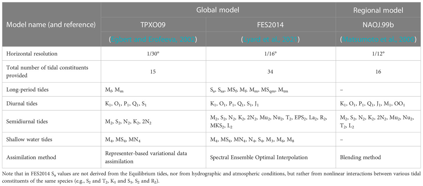
Table 1 Comparison of three online hydrodynamic models with data assimilation that produce open-access tidal harmonic constant databases.

While their data are readily accessible online, several simple but critical steps are required to process these data to ensure their successful use in regional and/or coastal ocean models. Firstly, before using the harmonic constants obtained from a larger domain tide database, phase lag references must be checked. In most global models and databases, phase lags are referenced to Greenwich (G) whereas most regional or coastal models tend to employ a local time zone reference (g), also termed the ‘local Greenwich phase lag’. Tidal constituent phase lags can be converted between Greenwich and local time zones using Eq. (5).

Secondly, THC data are commonly published at coarser resolutions than the grid dimensions of regional and coastal models. Accordingly, higher resolution tidal forcing inputs (i.e., $a_i$ and $G_i$) need to be accurately interpolated from the low-resolution THC data available from global databases. During interpolation, robust procedures are important for regions where THC dataset phase lags abruptly change across the 360˚ ‘boundary’ (e.g., from 350˚ to 10˚) over a certain number of grid points (Park et al., 2012). If these data are incorrectly interpolated, a systematic error can be introduced into the open boundary tidal forcings (Byun and Hart, 2017), as demonstrated in Figures 1 and 2.

FIGURE 1

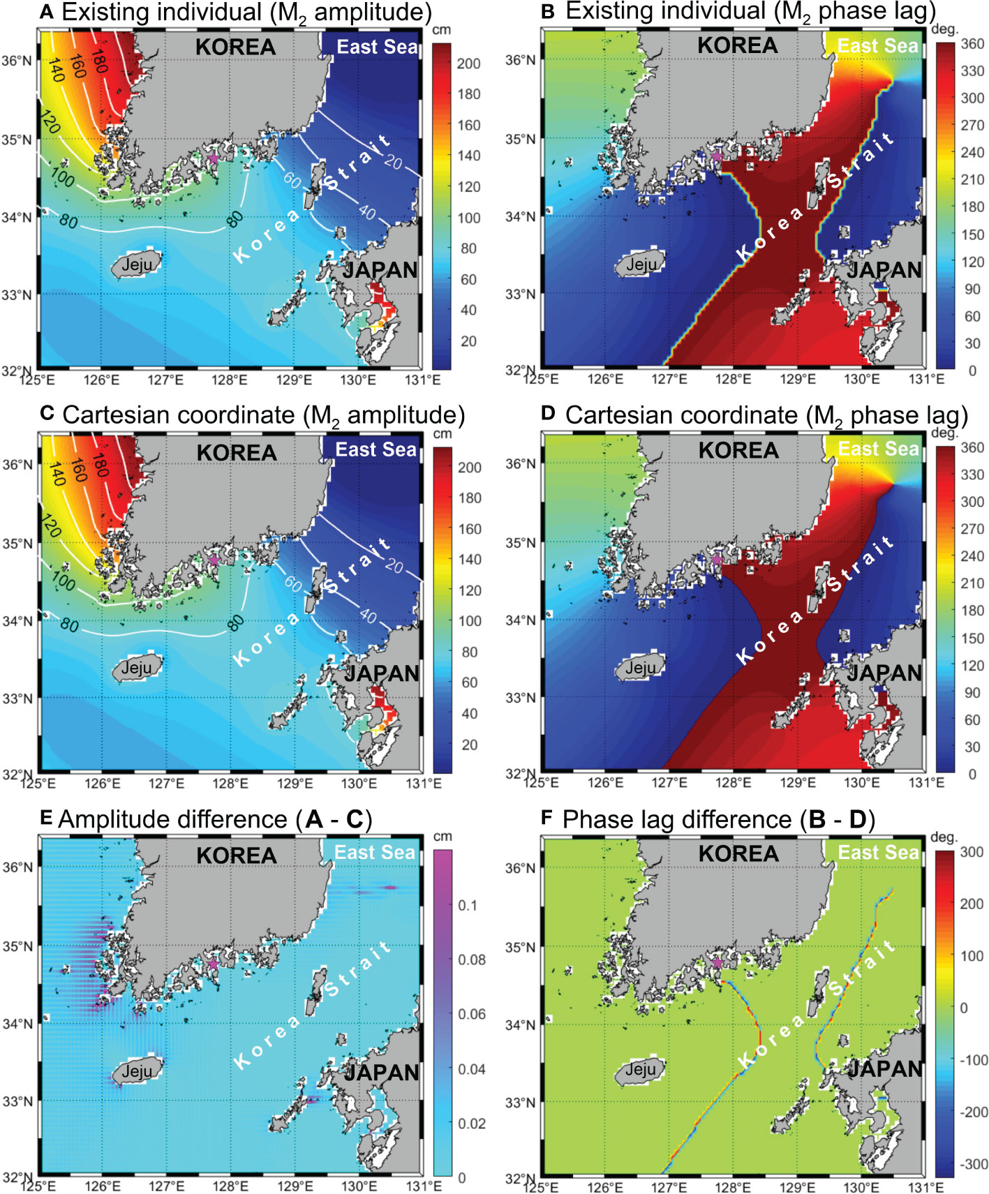
Figure 1 M₂ co-amplitude and cotidal charts (A–D) around Korea Strait produced using the existing individual linear interpolation method (A, B) and the Cartesian coordinate based linear interpolation method (C, D) with FES2014 tidal constant data (horizontal resolution of 1/16°). Plots (E, F) of the differences between the two interpolated charts (i.e., (A−C), and (B−D) are shown to highlight the errors introduced using the existing linear interpolation method (E, F). Phase lags are referenced to Greenwich. The magenta star indicates the location of Yeosu Tidal Station, which is operated by KHOA.

FIGURE 2

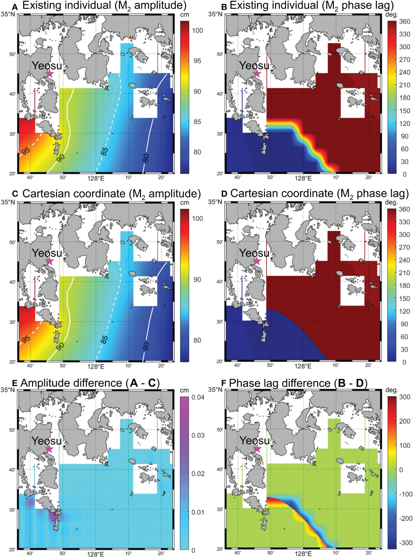
Figure 2 M₂ co-amplitude and cotidal charts (A–D) off Yeosu, Korea. The interpolated charts were produced using the existing individual linear interpolation method (A, B) and the Cartesian coordinate based linear interpolation (1/320°) method (C, D) from FES2014 tidal constant data (horizontal resolution of 1/16°). Differences between two interpolated charts (i.e., (A−C), and (B−D) are shown to highlight the errors introduced using the existing linear interpolation method (E, F). Phase lags are referenced to Greenwich. The magenta star indicates the location of Yeosu Tidal Station, which is operated by KHOA.

Interpolation problems can be easily avoided, as follows: Assuming the THCs for each tidal constituent at each model grid point comprise magnitudes and directions in polar coordinates, these coordinates should be converted to Cartesian coordinates. That is, the amplitudes ($a_i$) and phase lags ($G_i$) at each grid point are treated as vectors with magnitudes ($r_i$) and directions (${\phi }_i$) in polar coordinates. These polar coordinates, $r_i$ and ${\phi }_i$, can be trigonometrically converted to the Cartesian coordinates,

$x_i$ and $y_i$, whereby:

$\begin{array}{ll}(x_i, y_i)=(r_i\cos {\phi }_i, r_i\sin {\phi }_i)& (8)\end{array}$

Next, interpolation is conducted on each $x_i$ and $y_i$ value respectively. The resulting interpolated Cartesian coordinate values ($x{\text{'}}_i, y{\text{'}}_i$) are then converted back to polar coordinate values ($r{\text{'}}_i$, $\phi {\text{'}}_i$) to obtain correctly interpolated tidal constants ($a{\text{'}}_i$, $G{\text{'}}_i$) using the following equations:

$\begin{array}{ll}r{\text{'}}_i=a{\text{'}}_i=\sqrt{{(x{\text{'}}_i)}^2+{(y{\text{'}}_i)}^2}& (9)\end{array}$

$\begin{array}{ll}\phi {\text{'}}_i=G{\text{'}}_i=atan2(y{\text{'}}_i, x{\text{'}}_i)& (10)\end{array}$

Hereafter we call this successful interpolation approach ‘Cartesian Coordinate based Interpolation (CCI)’, while the pre-existing (sometimes erroneous) method is termed ‘Existing Individual Interpolation (EII)’. Figure 1 illustrates M₂ amplitude and phase lag charts produced using THC data generated via these two different approaches for Korea Strait. While the amplitudes produced using EII (Figure 1A) and CCI (Figure 1C) appear similar at first glance, amplitude differences greater than 0.1 cm exist around the islands off the southwest tip of Korea and in the vicinity of the East Sea M₂ amphidromic point (Figure 1E). Further, the phase lag results produced using EII contain incorrect interpolations across areas with abrupt phase lag changes, including around amphidromic points (e.g., Figure 1B), resulting in erroneous bands of phase lag difference (Figure 1F).

In contrast, phase lags are correctly interpolated without discontinuities using CCI (e.g., Figure 1D). Inaccurate model results can occur when using the EII method to interpolate tidal harmonic constants from a relatively coarse database to provide tidal forcings along the open boundaries of a high-resolution coastal model with abrupt phase lag changes. This is especially problematic if a significant proportion (e.g., >10%) of the interpolated grid points along the open boundary feature abrupt phase lag changes. In such cases, incorrect and out-of-phase tidal forcings can be produced over short distances along the open boundary. For example, when interpolating THCs from a coarse resolution global THC dataset like FES2014, which has a grid spacing of 1/16°, to a high-resolution coastal model domain with a grid spacing of 1/320° off Yeosu, Korea, errors may arise in the open boundary data for a certain number of grid points (Figure 2). Such errors can cause unexpected instability problems in the coastal ocean model.

Figure 2 illustrates the Yeosu coastal area as an example small domain with a high horizontal resolution (1/320°). For this small domain, when interpolating from FES2014 THC data with a horizontal grid spacing of 1/16°, approximately 15% of the interpolated grid points produced for the southern open boundary feature abrupt M₂ tide phase lag changes. Comparing the results of EEI and CCI based methods, relatively small differences exist between the interpolated amplitudes produced (Figure 2E) but significant differences arise between the interpolated phase lags (Figure 2F). As shown in Figure 2F, if incorrectly interpolated phase lags are included in the open boundary tidal forcing files, these errors can propagate into the nested model domain over time.

For the relatively large Korea Strait domain, with its comparatively lower grid resolution (1/48°), we calculated the maximum differences between M₂ constituent THCs produced using the two interpolation methods for grid points at each latitudinal band. Differences were found to be as large as 0.6 cm and 80 to 240°, respectively, in the interior of the domain (Figures 3A, B). Differences between the two methods’ tidal amplitude results along the southern boundary were smaller than 0.006 cm (Figure 3C), and there was a discontinuity in tidal phase lag over two grid points (Figure 3D). However, in the relatively small Yeosu coastal area domain, with its comparatively high grid resolution (1/320°), the differences produced using the two methods for tidal amplitudes along the southern boundary were smaller than 0.012 cm (Figure 3E), with an abrupt change in tidal phase lag occurring over ~15% of the grid points (39 out of a total 257 grid points) along the southern boundary (Figures 3C–F).

FIGURE 3

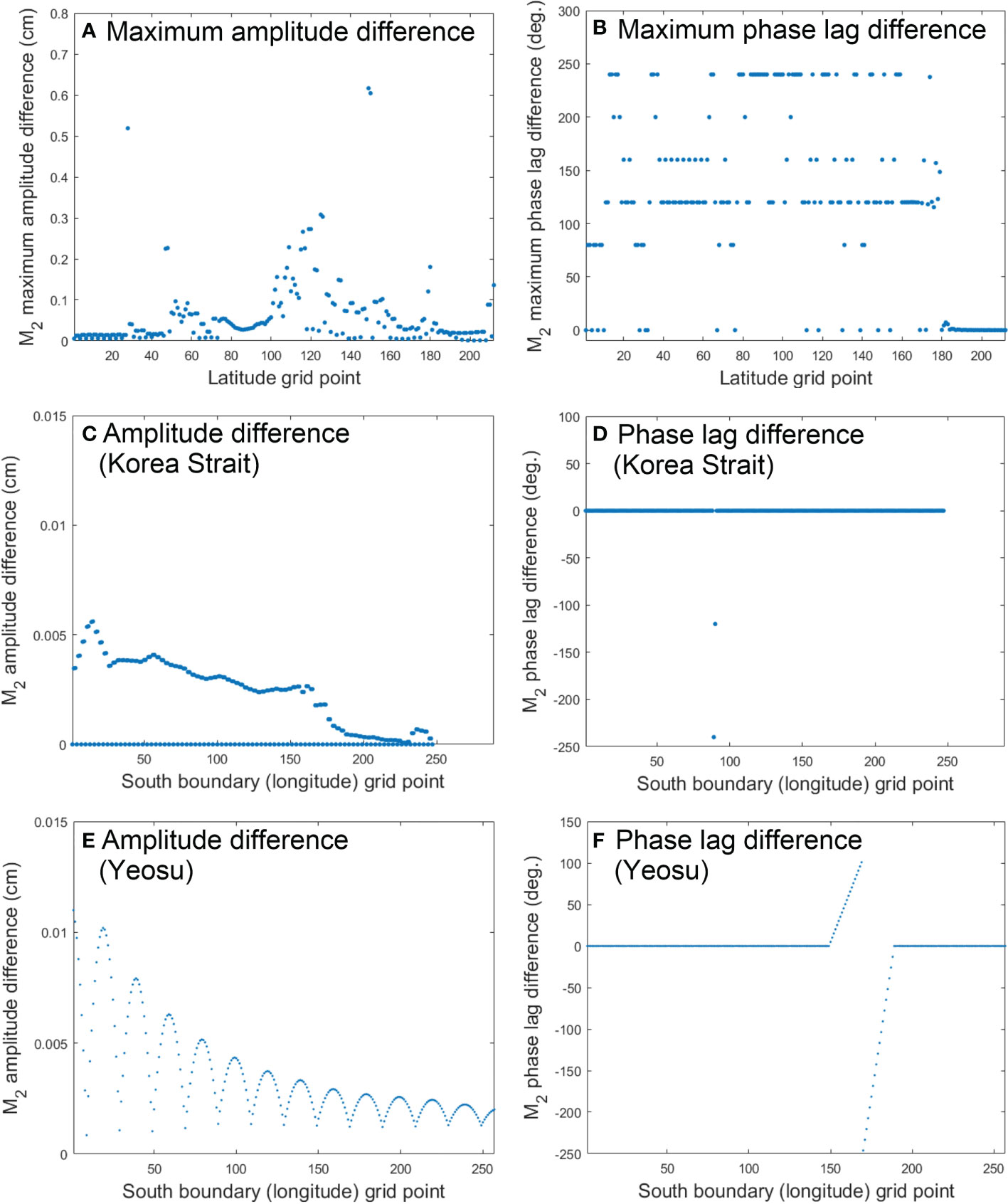
Figure 3 Maximum differences in amplitude and phase lag of the M₂ constituent (A, B) along longitudinal girds at each latitudinal grid point, derived from Figures 1E, F. Differences in amplitudes and phase lags along southern boundary of the Korea Strait domain (C, D) of Figure 1 and in the Yeosu coastal domain (E, F) of Figure 2.

Xu (2018) also demonstrates, using a relatively extreme theoretical example, how individual and linear treatment of amplitudes and phase lags can lead to very different, incorrect results compared to vector-based non-linear interpolations. Our CCI approach produces the same interpolation results as Xu (2018) method. Furthermore, our realistic test cases comparing results produced using EII versus CCI generated THCs reveal that the comparative coarseness of the THCs database versus the size of the model domain for which the tidal forcings are being produced does matter. Irrespective of this new understanding, since the CCI approach is universally more robust then EII, and since it is easy to perform, we strongly recommend its use (instead of EII) for all TCC interpolations for regional coastal ocean models.

To avoid tidal harmonic constant interpolation problems, model databases such as TPXO09 (Egbert and Erofeeva, 2002) provide data in the form of complex numbers ($z_i)$ with real $(X_i)$ and imaginary $(Y_i)$ parts, rather than as THCs (amplitudes and phase lags). The procedure for obtaining tidal harmonic constant model input data from these complex numbers is equivalent to that used with Cartesian coordinates as explained in Eq. (8), since this form of complex number, termed Cartesian representations, can be expressed as polar representations ($r_i$) according to:

$\begin{array}{ll}{z}_i=X_i+i{Y}_i=a_i(\cos G_i+i\sin G_i)& (11)\end{array}$

Firstly, interpolation is conducted on each $X_i$ and $Y_i$ data, respectively, resulting in interpolated real $(X_i^{\text{'}})$ and imaginary $(Y_i^{\text{'}})$ data. Then, using ($X_i^{\text{'}}, Y_i^{\text{'}}),$the interpolated amplitude ($a{\text{'}}_i$) and phase lag ($G{\text{'}}_i$) for a constituent can be calculated via: for amplitude

$\begin{array}{ll}a{\text{'}}_i=\left|z_i^{\text{'}}\right|=\sqrt{{(X_i^{\text{'}})}^2+{(Y_i^{\text{'}})}^2}& (12)\end{array}$

for phase lag

$\begin{array}{ll}{G}_i^{\text{'}}=\arg (z_i^{\text{'}})=atan2(y{\text{'}}_i, x{\text{'}}_i)& (13)\end{array}$

In reverse, the tidal harmonic constants derived from a tidal model simulation can be converted into complex numbers using Eq. (11) as follows:

$\begin{array}{ll}\text{Re}\left\{z_i^{\text{'}}\right\}=X_i=a{\text{'}}_i cos{G}_i^{\text{'}}& (14)\end{array}$

$\begin{array}{ll}\text{Im}\left\{z_i^{\text{'}}\right\}=Y_i=a{\text{'}}_i sin{G}_i^{\text{'}}& (15)\end{array}$

4 Long-term perpetual interannual tidal prediction

4.1 Key factors for long-term tidal prediction

When applying a hydrodynamic model to tide-dominated continental shelves or shallow coastal seas, like the Yellow and East China Seas, and around Antarctica where different tidal regimes coexist (Figure 4A), frequently updated NMC factors ($f_i$ and $u_i$) are needed for robust perpetual interannual simulations (Byun and Cho, 2009). The question arises: Why do NMC need such treatment for accurate tidal predictions in these tidal regimes? To elucidate, we used T_Tide’s t_vuf.m function (Pawlowicz et al., 2002), to examine variations in the daily NMC factors for three major lunar tide constituents (K₁, O₁ and M₂) over a 40 year period for Yeosu, Korea, as illustrated in Figure 4. Variations in the diurnal O₁ tide NMC were the largest, with the $f_{O_1}$and $u_{O_1}$ ranges being 0.387 (0.800 ~ 1.187) and 22.56° (-11.35° ~ 11.21°), respectively. Variations in K₁ tide NMC were second largest, with the ranges of $f_{K_1}$and $u_{K_1}$ being 0.232 (0.881 ~ 1.113) and 17.82° (-8.89° ~ 8.93°), respectively. In contrast, variation in the semidiurnal M₂ tide’s NMC were relatively small, with the $f_{M_2}$ and $u_{M_2}$ ranges being 0.075 (0.963 ~ 1.038) and 4.28° (-2.02° ~ 2.26°), respectively.

FIGURE 4

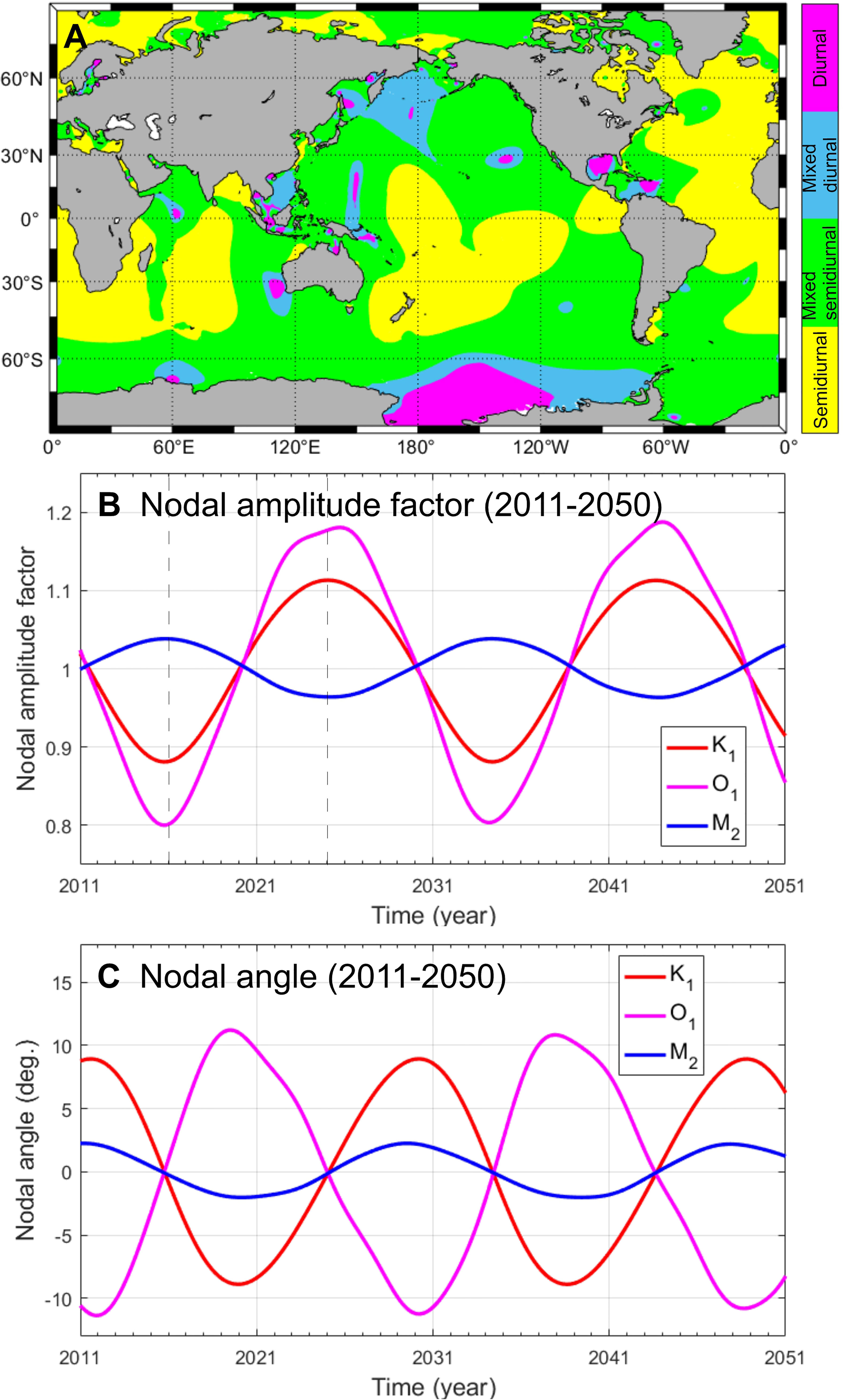
Figure 4 Map of (A) global distribution of semidiurnal (F<0.25), mixed mainly semidiurnal (0.25<F<1.5), mixed mainly diurnal (1.5<F<3.0) and diurnal tides (F>3.0) (classified using the tidal form factor amplitude ratio of F=(K₁+O₁)/(M₂+S₂)), using the FES2014 model database of tidal harmonic constants. Variation in nodal amplitude factors (B) and nodal angles (C) of the three main lunar tidal constituents (K₁, O₁ and M₂) from 2011 to 2050 at Yeosu, on the central south coast of Korea (see location in Figure 1), estimated at daily intervals using T_Tide’s t_vuf.m program (Pawlowicz et al., 2002).

The implications of these NMC factor variations differ for different regions, such as around Antarctica versus in the East Sea (Figure 4A), since these environments are characterized by different kinds of tidal conditions, including semidiurnal versus diurnal tide dominance (Byun and Hart, 2020; Byun and Hart, 2022). The resulting variations in tidal heights are less pronounced in semidiurnal versus diurnal regimes, with the latter experiencing much larger tidal range variations over 18.61 yr cycles due to the influence of diurnal nodal factor variation, which is greater than that of the semidiurnal M₂ tide (e.g., compare nodal amplitude factors between 2006 and 2015 in Figure 4B). Of note, variations in $f_{O_1}$ and $f_{K_1}$ are out of phase with that of $f_{M_2}$ while variation in $u_{K_1}$is in phase with that of $u_{M_2}$ but not with that of $u_{O_1}$ (Figure 4C).

Another consideration is whether theoretically calculated NMC factor values can represent actual observed oceanic tide variations. To illustrate this, a time series of the K₁, O₁ and M₂ constituents’ harmonic constants was calculated at annual intervals without NMC, using tidal harmonic analysis over 52 years (1969-2020) at Yeosu. Results indicate the existence of nodal modulation effects that are similar to the theoretically proposed variations (Figure 5). The major lunar tidal harmonic constants (amplitudes and phases) calculated from the observed annual sea level data varied across the 18.61 yr nodal cycle. In comparison with the variations in K₁ tidal amplitudes, those of the O₁ were larger and their phase lags were 180° out of phase (Figures 5A–D).

FIGURE 5

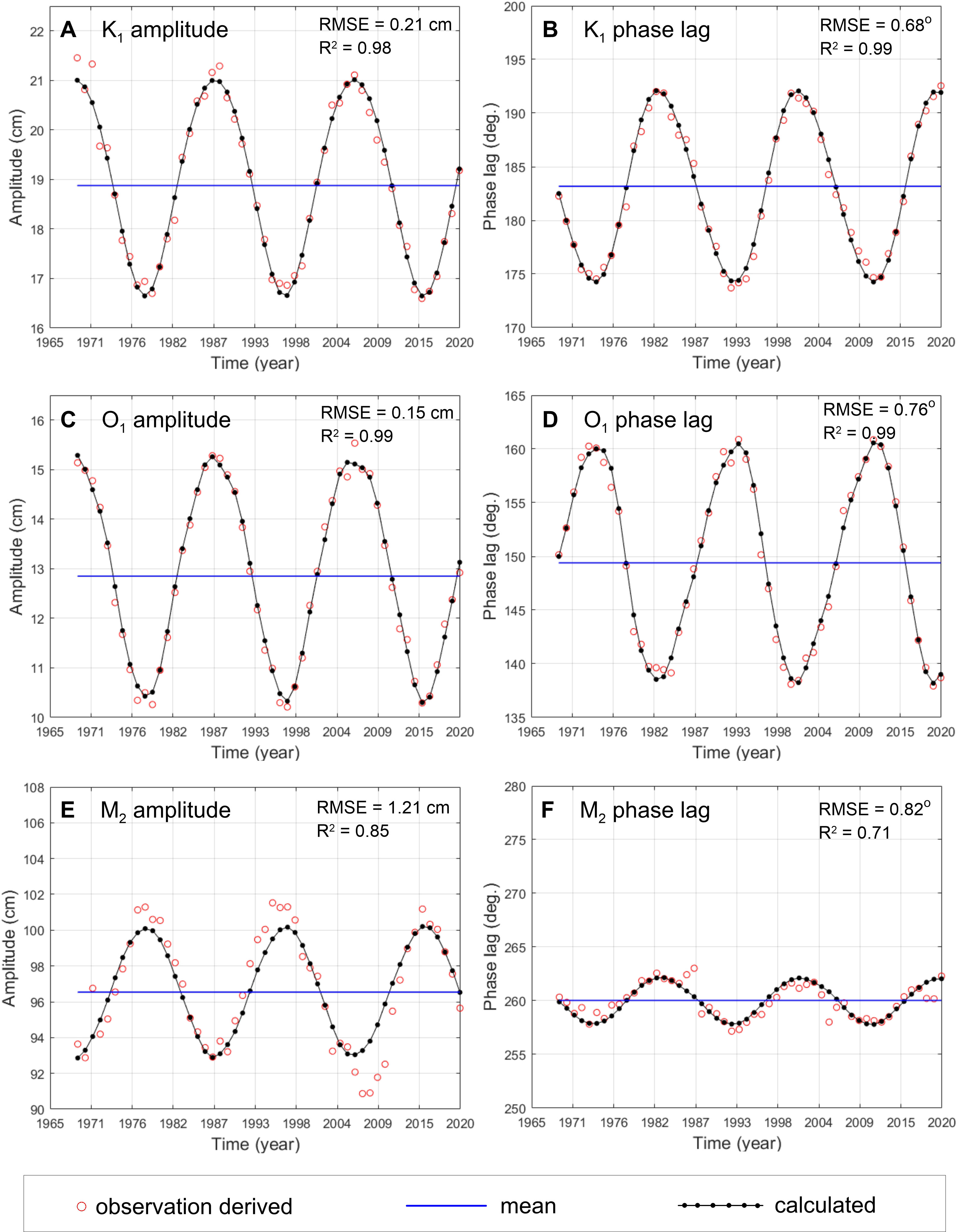
Figure 5 Annual variation in amplitudes (A, C, E) and phase lags (B, D, F) for the three main lunar tidal constituents (K₁, O₁ and M₂) from 1969 to 2020 at Yeosu, Korea. Red open circles are the harmonic constants estimated using year-long observation records with T_Tide (Pawlowicz et al., 2002), without nodal modulation correction (i.e., with single nodal amplitude factor and nodal angle values employed for each constituent from the middle of each observation year). Blue lines are the mean tidal constants over the entire 52-year record. The black solid dots on black lines are the annual harmonic constants calculated by multiplying the mean tidal constants by the nodal amplitude factors and nodal angles for each year as derived from T_Tide’s t_vuf.m program. Note that linear trends were removed from the M₂ tidal constants only.

Root mean square errors (RMSEs) and coefficients of determination (R²) between the observed and theoretically determined tidal constants for the two diurnal tidal constituents (K₁ and O₁) were calculated to verify their similarity. The RMSE and R² results were 0.21 cm and 0.98 for the K₁ amplitude, 0.68° and 0.99 for the K₁ phase lag, 0.15 cm and 0.99 for the O₁ amplitude, and 0.76° and 0.99 for the O₁ phase lag, respectively. For the M₂, the RMSE and R² values were 1.21 cm and 0.85 for the amplitude and 0.82° and 0.71 for the phase lag, respectively. These results suggest that the theoretical values used in tidal prediction can successfully represent nodal modulation. Similarly, Feng et al. (2015)’s results confirmed that long-term annual harmonic analysis results for the main tidal constituents along China’s Yellow and East China Sea coasts agreed with theoretically determined results.

Two general approaches exist for including NMC in ocean model tidal predictions: (1) external calculation of fixed (e.g., model start-time) NMC factors ($f_i$ and $u_i$) and astronomical arguments ($V_i$) during the generation of tidal forcing input data; and (2) internal, continuous, online updates of NMC factors during model simulations, using pre-processed tidal harmonic constants. When simulating only one or two years of tidal data, using externally generated, fixed NMC factors based on input tidal forcing data (i.e., 1) can prove an efficient approach, with only minor errors.

For example, as pointed out by Byun and Cho (2009), a regional ocean circulation model such as ROMS usually uses fixed NMC factors calculated once, with tidal forcing input data generated at start time and no subroutine for NMC updates in the model. A better approach when using ROMS is to externally calculate NMC factors once for the middle of the prediction time, and to combine this with continuous tidal constant adjustments using the NMC factors across the entire tidal prediction period. This is an acceptable approach for simulations of <1 year since $f_i$ and $u_i$ change slowly across the18.61 year nodal cycle (Figure 2), which is similar to the tidal prediction approach used in T_TIDE, as demonstrated by Byun and Hart (2019).

Such a simple approach is, however, inappropriate for longer-term perpetual tidal predictions. The use of fixed NMC factors means this approach can produce significant errors if used, for example, in multi-decadal or other long-term simulations of the ocean climate or in ocean operating systems. Instead, NMC factors should be continuously updated (at least at annual timescales) to produce accurate variations in tidal harmonic constants when attempting to simulate the tides and processes they affect over timeframes greater than two years.

4.2 Long-term perpetual interannual tidal prediction

Over decadal scale studies, frequent NMC factor updates are required to produce accurate perpetual tidal simulations (Howard et al., 2019) or to predict nuisance or extreme flooding risks (Ray and Foster, 2016; Talke et al., 2018). Accuracy can be achieved in regional ocean models by including NMC effects in either external or internal tidal forcings, with the correct assignment of time stamps in configuration files, such as in ‘roms.in’. Another effective approach is to employ a new external tidal forcing file for each simulated year, with these files containing new tidal harmonic constants produced using mid-year estimates of the lunar tidal constituents’ nodal amplitude factors and nodal angles.

To overcome NMC issue, a well-known and relatively simple conventional tidal prediction algorithm such as TASK-2000’s ‘marie.f’ (Bell et al., 1999) can be adopted in regional tidal predictions. In ROMS, this subroutine can be included in the ‘ROMS\Nonlinear\set_tides.F’ file to calculate the lunar tidal constituents’ astronomical arguments ($V_i$), nodal amplitude factors ($f_i$) and nodal angles ($u_i$) internally over the period covered by model simulations. In ‘marie.f’, algorithms for calculating the five fundamental astronomical variables can be replaced by those of Foreman (1977) for predictions covering the years 1801 to 2099, to overcome leap year time parameterization issues (Byun, 2010). Refer to Byun and Cho (2009) for more details on the importance of NMC effects in coastal ocean model tidal prediction. This paper’s Supplementary Material contains a modified version of ‘set_tides.F’ for use in ROMS that solves both the frequent NMC effect issue of the original, with this new code successfully tested in the ROMS 4.0 trunk version 1108.

For any robust tidal forecasting simulation (e.g., from multi-decadal forecasting simulations through to a couple of days of operational simulations) in ROMS using either external or internal NMC, it is important that times stamps are correctly characterized in ‘roms.in’. For example, ‘roms.in’ contains standard input parameters for ROMS execution after compiling. Therein it is essential that time stamp variables are employed correctly, including for model initialization (DSTART), the tidal forcing start time (TIDE_START), and for model output reference times in NetCDF format (TIME_REF). For typical perpetual interannual tidal predictions using the modified ‘set_tides.F’, ‘TIME_REF = -2’ is employed, which refers to time elapsed ($\tau -{\tau }_0$) since 1968-05-23 (i.e., Julian day 2440000), the program default start time (${\tau }_0=$ 2440000 days). ‘DSTART’ value is calculated in MATLAB as a modified Julian date of the start time (YYYY MM DD) according to ‘juliandate ([YYYY MM DD])– 2440000’ (a modification that reduces day digital numbers). For example, if DSTART=19618 days, this means that the ROMS starts on February 7, 2022, according to ‘datevec(DSTART+ ${\tau }_0$)’ in MATLAB. For our modified version of ‘set_tides.F’, ‘TIDE_START is unutilized, such that it is given as TIDE_START=0.

5 Production of tidal harmonic constant databases for regional oceans

As noted earlier, high spatial resolution tidal harmonic constant data are needed to model tides and tidal currents in regional and coastal ocean settings. A tidal harmonic constant database can be produced to provide the tidal forcing input data required for such ocean models using (1) a tide model generated hourly predicted tidal height data at each grid point, and (2) harmonic analysis of these data to calculate their harmonic constants.

The latter harmonic analysis step is similar to that performed on sea level observation records. Three key points must be carefully checked to ensure reliable tidal harmonic constants are generated in such simulations: (1) whether NMC effects have been included properly or excluded from model simulations; (2) the minimum length of simulated tidal height data required for harmonics analysis to produce the tidal harmonic constants needed; and (3) the phase lag time zone employed.

Firstly, when a model is used to simulate tides based on Eq. (3) or (4) with NMC factors and astronomical arguments, a conventional tidal harmonic analysis program (e.g., Task-2000, IOS, T_TIDE and UTide) can be used to produce a tidal constant database. Note that each tidal analysis and prediction package employs their own tidal constituent notations and slightly different angular speeds (e.g., ${\omega }_{M}1$= 14.4920521° hr^-1 in Task-2000 versus ${\omega }_{NO}1$= 14.4966939° hr^-1 in IOS, T_TIDE and UTide; or ${\omega }_{S}a$= 0. 0410686° hr^-1 in Task-2000 versus ${\omega }_{S}a$= 0.0410667° hr^-1 in IOS, T_TIDE and UTide. S_a angular speed differences, for example, are produced by exclusion or inclusion of the perihelion term, which modifies the S_a constituent phase lag by 0.0000019617° hr^-1. These different tide model approaches have significant effects on calculated phase lags: for example, Byun et al. (2021) found a 77° difference in the S_a phase lag results produced using IOS (T_TIDE and UTide) and Task-2000 for the year 2000. Identical tidal constituent names and periods should be employed in the tidal analysis program used to calculate the tidal harmonic constants and/in the regional ocean tide model for which these tidal forcing data are produced. In addition, when tidal model simulations exclude NMC factors and astronomical arguments, the harmonic constants used in the model’s tidal forcing can be extracted using least-squares fitting.

The question arises as to what duration of simulated elevation data are needed to obtain the tidal constants of the constituents employed in the initial harmonic analysis. Pairs of neighboring constituents (i, j) with similar angular speeds (${\omega }_i$, ${\omega }_j$) can be separated out using data spanning their synodic period (SP), as calculated by:

$\begin{array}{ll}SP(i,j)=\frac{360°}{{\omega }_i-{\omega }_j}& (14)\end{array}$

(Pugh and Woodworth, 2014) and listed in Table 2. For example, for a model run using the four major tidal constituents (M₂, S₂, K₁ and O₁), at least 15 days of hourly tidal height outputs are required for subsequent harmonic analysis of these data to produce accurate tidal constant results, including separation of the M₂ and S₂ constituents. Note that when beginning the model from a ‘cold start’, additional spin up time should be added to the minimum model run time needed to separate neighboring.

TABLE 2

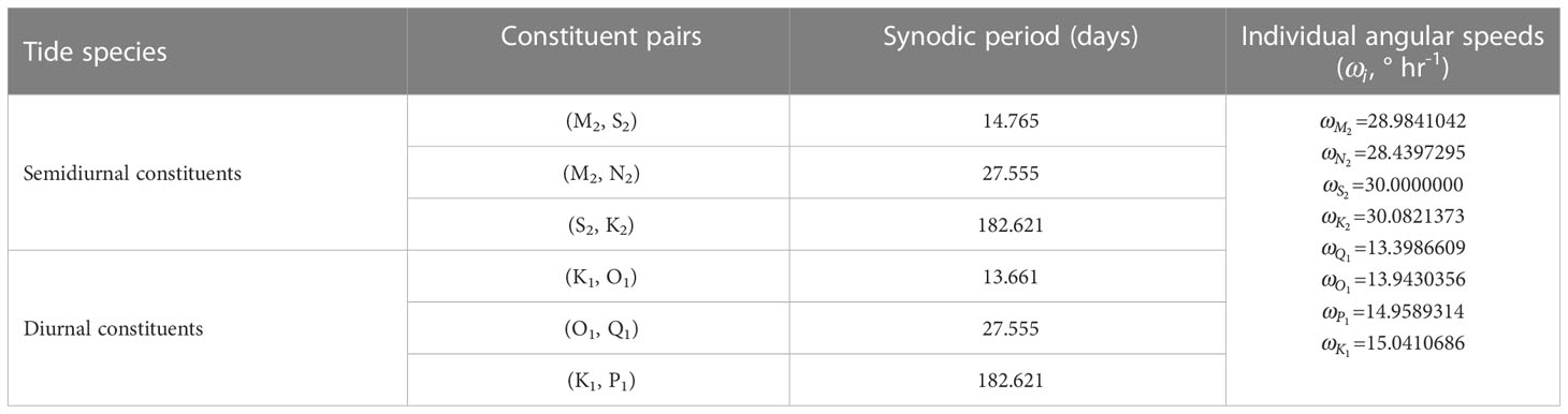
Table 2 Key pairs of neighboring semidiurnal and diurnal constituents and their synodic periods (which correspond to the modeled sea level dataset durations required to separate out paired constituents via conventional harmonic analysis), and individual constituent angular speeds.

In addition, when a model is run with the eight major tidal constituents (M₂, S₂, N₂, K₂, K₁, O₁, P₁, and Q₁), at least 183 days of modeled tidal height data are needed to separate neighboring constituent pairs such as the semidiurnal S₂ and K₂ tides and the diurnal K₁ and P₁ tides (Byun, 2011).

Lastly, the tidal constituents’ phase lag reference should be indicated, based on the time zone used in model simulations. When local time zones (Greenwich mean time zone) are used in simulations, the harmonically analyzed phase lags must also be referenced to this time zone.

6 Summary

This work provides robust technical guidance for researchers wanting to successfully establish regional or coastal ocean forecasting systems with embedded tidal processes. Of significance, advice is provided for achieving accurate perpetual multi-decadal tidal predictions, as needed in studies of future ocean climate changes and/or tidal inundation risks in tide dominated environments. This work includes essential information for (1) generating accurate high resolution tidal forcing inputs for models based on coarse resolution tidal constant databases, and (2) the steps required for producing accurate long-term perpetual tidal predictions (Figure 6). By way of a practical solution, an approach for tidal prediction in ROMS is provided (including a modified set_tides.F code, in the Supplementary Material), resolving issues associated with using this model for continuous long-term tidal predictions. A successful procedure is explained for producing the tidal harmonic constants needed as regional and coastal ocean model input data, based on tidal heights simulated by a tide model.

FIGURE 6

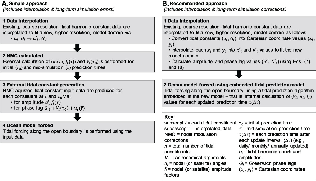
Figure 6 Comparison of (A) simple (error prone) and (B) improved alternative (standard harmonic prediction based) methodological procedures for generating the tidal forcings file needed to predict tides in regional and coastal ocean models.

Data availability statement

Publicly available datasets were analyzed in this study. This data can be found here: The FES2014 model database of tidal harmonic constants used in this study can be found via https://www.aviso.altimetry.fr/en/data/products/auxiliary-products/global-tide-fes.html. The Yeosu sea level observation data used in this work can be downloaded from the Korea Hydrography and Oceanographic Agency (KHOA) online data repository via http://khoa.go.kr/oceangrid/gis/category/reference/.

Author contributions

All authors conceived this paper including the manuscript structure and content. D-SB wrote the first draft of manuscript and DH and B-JC reviewed, edited and improved the manuscript. D-SB completed the tidal prediction code for ROMS with B-JC’s help. All authors contributed to the article and approved the submitted version.

Funding

The KHOA is thanked for financial support (2000-2033-307-210-13) in publishing this paper. B-J Choi was supported by Korea Institute of Marine Science & Technology Promotion (KIMST) funded by the Ministry of Oceans and Fisheries (20220033).

Acknowledgments

Thank you to the Korea Hydrographic and Oceanographic Agency (KHOA) and CNES/AVISO+ for providing observation and model data, and to Dr. Jong-Kyu Kim for supporting the Korea Strait model test experiments conducted in response to reviewer questions. Thank you also to the three reviewers for their comments, which helped us improve our manuscript.

Conflict of interest

The authors declare that the research was conducted in the absence of any commercial or financial relationships that could be construed as a potential conflict of interest.

Publisher’s note

All claims expressed in this article are solely those of the authors and do not necessarily represent those of their affiliated organizations, or those of the publisher, the editors and the reviewers. Any product that may be evaluated in this article, or claim that may be made by its manufacturer, is not guaranteed or endorsed by the publisher.

Supplementary material

The Supplementary Material for this article can be found online at: https://www.frontiersin.org/articles/10.3389/fmars.2023.1150305/full#supplementary-material

References

Bell C., Vassie J. M., Woodworth P. L. (1999). POL/PSMSL tidal analysis software kit 2000 (TASK-2000) (Birkenhead, UK: Permanent Service for Mean Sea Level, CCMS Proudman Oceanographic Laboratory, Bidston Observatory), 20.

Google Scholar

Blain C. A., Preller R. H., Rivera A. P. (2002). Tidal prediction using the advanced circulation model (ADCIRC) and a relocatable PC-based system. Oceanography 15 (1), 77–87. doi: 10.5670/oceanog.2002.38

CrossRef Full Text | Google Scholar

Byun D.-S. (2010). Exploring estimation of paleo-tides and -tidal currents using a harmonic analysis method in pre-19th century (in Korean). J. Korean Soc Oceanogr. 15 (4), 203–206.

Google Scholar

Byun D.-S. (2011). Investigating the adjustment methods of monthly variability in tidal current harmonic constants (in Korean). Ocean Polar Res. 33, 309–319. doi: 10.4217/OPR.2011.33.3.309

CrossRef Full Text | Google Scholar

Byun D.-S., Cho C. W. (2009). Exploring conventional tidal prediction schemes for improved coastal numerical forecast modeling. Ocean Model. 28, 193–202. doi: 10.1016/j.ocemod.2009.02.001

CrossRef Full Text | Google Scholar

Byun D.-S., Choi B.-J., Kim H. W. (2021). Non-astronomical tides and monthly mean Sea level variations due to differing hydrographic conditions and atmospheric pressure along the Korean coast from 1999 to 2017 (in Korean). J. Korean Soc Oceanogr. 26 (1), 11–36. doi: 10.7850/jkso.2021.26.1.011

CrossRef Full Text | Google Scholar

Byun D.-S., Hart D. E. (2017). On robust multi-year tidal prediction using T_TIDE. Ocean Sci. J. 54 (4), 657–671. doi: 10.1007/s12601-019-0036-4

CrossRef Full Text | Google Scholar

Byun D.-S., Hart D. E. (2020). Predicting tidal heights for extreme environments: from 25 h observations to accurate predictions at jang bogo Antarctic research station, Ross Sea, Antarctica. Ocean Sci. 16, 1111–1124. doi: 10.5194/os-16-1111-2020

CrossRef Full Text | Google Scholar

Byun D.-S., Hart D. E. (2022). Tidal current classification insights for search, rescue and recovery operations in the yellow and east China seas and Korea strait. Continental Shelf Res. 232, 1–14. doi: 10.1016/j.csr.2021.104632

CrossRef Full Text | Google Scholar

Byun D.-S., Hart D. E.. (2017). A robust interpolation procedure for producing tidal current ellipse inputs for regional and coastal ocean numerical models. Ocean Dynamics 67, 451–63. doi: 10.1007/s10236-017-1037-4

CrossRef Full Text | Google Scholar

Byun D.-S., Seo G.-H., Park S.-Y., Jeong K.-Y., Lee J. Y., Choi W.-J., et al. (2017). A technical guide to operational regional ocean forecasting systems in the Korea hydrographic and oceanographic agency (I): Continuous operation strategy, downloading external data, and error notification (in Korean). J. Korean Soc Oceanogr. 22 (3), 91–105. doi: 10.7850/jkso.2017.22.3.091

CrossRef Full Text | Google Scholar

Egbert G. D., Erofeeva S. Y. (2002). Efficient inverse modeling of barotropic ocean tides. J. Atmos. Ocean. Tech. 19 (2), 183–204. doi: 10.1175/1520-0426(2002)019<0183:EIMOBO>2.0.CO;2

CrossRef Full Text | Google Scholar

Feng X., Tsimplis M. N., Woodworth P. L. (2015). Nodal variations and long-term changes in the main tides on the coasts of China. J. Geophys. Res. Oceans 120, 1215–1232. doi: 10.1002/2014JC010312

CrossRef Full Text | Google Scholar

Foreman M. G. G. (1977). Manual for tidal heights analysis and prediction Vol. 77-10 (Sidney, B.C.: Institute of Ocean Sciences, Pacific Marine Science Report), 97.

Google Scholar

Howard T., Palmer M. D., Bricheno L. M. (2019). Contributions to 21st century projections of extreme sea-level change around the UK. Environ. Res. Commun. 1, 095002. doi: 10.1088/2515-7620/ab42d7

CrossRef Full Text | Google Scholar

Huang W., Zhang Y. J., Wang Z., Ye F., Moghimi S., Myers E., et al. (2022). Tidal simulation revisited. Ocean Dynamics 72, 187–205. doi: 10.1007/s10236-022-01498-9

CrossRef Full Text | Google Scholar

Kim Y.-Y., Kim B.-G., Jeong K. Y., Lee E. L., Byun D.-S., Cho Y.-K. (2021). Local Sea-level rise caused by climate change in the Northwest pacific marginal seas using dynamical downscaling. Front. Mar. Sci. 8. doi: 10.3389/fmars.2021.620570

CrossRef Full Text | Google Scholar

Lee K. J., Nam S. H., Cho Y.-K., Jeong K.-Y., Byun D.-S. (2022). Determination of long-term, (1993–2019) Sea level rise trends around the Korean peninsula using ocean tide-corrected, multi-mission satellite altimetry data. Front. Mar. Sci. 9. doi: 10.3389/fmars.2022.810549

PubMed Abstract | CrossRef Full Text | Google Scholar

Loder J. W., Garrett C. (1978). The 18.6-year cycle of sea surface temperature in shallow seas due to variations in tidal mixing. J. Geophysical Res. 83, 1967–1970. doi: 10.1029/JC083iC04p01967

CrossRef Full Text | Google Scholar

Lyard F. H., Allain D. J., Cancet M., Carrère L., Picot N. (2021). FES2014 global ocean tide atlas: design and performance. Ocean Sci. 17, 615–649. doi: 10.5194/os-17-615-2021

CrossRef Full Text | Google Scholar

Madec G., NEMO-team (2022). NEMO ocean engine, scientific notes of climate modelling center (Paris, France: Institut Pierre-Simon Laplace (IPSL). doi: 10.5281/zenodo.1464816

CrossRef Full Text | Google Scholar

Matsumoto K., Takanezawa T., Ooe M. (2000). Ocean tide models developed by assimilating TOPEX/POSEIDON altimeter data into hydrodynamical model: A global model and a regional model around Japan. J. Oceanogr 56, 567–581. doi: 10.1023/A:1011157212596

CrossRef Full Text | Google Scholar

Park S.-Y., Byun D.-S., Hart D. E. (2012). A solution for the correct interpolation of data across regions with abrupt changes in tidal phase-lag. Ocean Sci. J. 47, 215–219. doi: 10.1007/s12601-012-0022-6

CrossRef Full Text | Google Scholar

Pawlowicz R., Beardsley B., Lentz S. (2002). Classical tidal harmonic analysis including error estimates in MATLAB using T_TIDE. Comput. Geosci 28, 929–937. doi: 10.1016/S0098-3004(02)00013-4

CrossRef Full Text | Google Scholar

Penven P., Marchesiello P., Debreu L., Lefèvre J. (2008). Software tools for pre- and post-processing of oceanic regional simulations. Environ. Model. Software 23 (5), 660–662. doi: 10.1016/j.envsoft.2007.07.004

CrossRef Full Text | Google Scholar

Pugh D., Woodworth P. (2014). Sea-Level science: Understanding tides, surges, tsunamis and mean sea-level changes (Cambridge, United Kingdom: Cambridge University press), 394. doi: 10.1017/CBO9781139235778

CrossRef Full Text | Google Scholar

Ray R. D., Foster G. (2016). Future nuisance flooding at Boston caused by astronomical tides alone. Earth’s Future 4, 578–587. doi: 10.1002/2016EF000423

CrossRef Full Text | Google Scholar

Seo G.-H., Cho Y.-K., Choi B.-J. (2014). Variations of heat transport in the northwestern pacific marginal seas inferred from high-resolution reanalysis. Prog. Oceanogr. 121, 98–108. doi: 10.1016/j.pocean.2013.10.005

CrossRef Full Text | Google Scholar

Talke S., Kemp A., Woodruff J. (2018). Relative sea level, tides, and extreme water levels in Boston harbor from 1825 to 2018. J. Geophysical Research: Oceans 123, 3895–3914. doi: 10.1029/2017JC013645

CrossRef Full Text | Google Scholar

Xu Z. (2018). A note on interpreting tidal harmonic constants. Ocean Dynamics 68, 211–222. doi: 10.1007/s10236-017-1122-8

CrossRef Full Text | Google Scholar