Opportunities and limitations of large open biodiversity occurrence databases in the context of a Marine Ecosystem Assessment of the Southern Ocean

1 Introduction

The Southern Ocean is a highly productive region that provides a large variety of ecosystem services (e.g., climate regulation, natural resources – including for food provision – and tourism; Grant et al., 2013). Exploration and exploitation of the Southern Ocean is relatively recent (starting with small research and whaling expeditions at the end of the 19th century) but interest and human activities have since increased dramatically, along with associated stressors – e.g., exploitation of fishing resources, disturbances by human visitors, pollution, invasive species, but also global warming and ocean acidification (Petrou et al., 2019; Rogers et al., 2020; Grant et al., 2021). Changes induced by these stressors can be profound and are expected to become more important (e.g., changes in primary productivity, ecosystem structure and functions, carbon uptake, species migrations, etc.; Henley et al., 2020; Morley et al., 2020; Brasier et al., 2021; Caccavo et al., 2021). For these reasons, maintaining the Southern Ocean in good health by minimizing the impact of human activities and climate change on ecosystem services should be a major priority for governance and policy bodies (Kennicutt et al., 2014; Rogers et al., 2020).

In this context, a marine ecosystem assessment of the Southern Ocean (MEASO) aims to provide managers with consolidated information about the status and trends of Southern Ocean habitats, species and ecosystems, to better support management and conservation planning activities. This information includes summaries of current knowledge from experts and peer-reviewed literature as well as biodiversity-related data and model outputs that can inform specific aspects of policy development. The specific requirements of such data will vary according to the particular objectives of a given assessment exercise. Ideally, however, biodiversity data should include abundances or densities from a phylogenetically and functionally wide variety of species, have a circumpolar coverage and allow comparison of the present state with a past benchmark (Brasier et al., 2019). As a starting point, the Census of Antarctic Marine Life (Schiaparelli et al., 2013) had as its main objective to understand the biodiversity of the Southern Ocean and set reference baselines to allow subsequent measurements of change (Van de Putte et al., 2021). The resulting Biogeographic Atlas of the Southern Ocean ( de Broyer and Koubbi, 2014) provided an initial benchmark of the Southern Ocean biogeography knowledge. However, to inform policy, such complex ecological data are best summarised in a few easily understandable statistics which can be used to track changes through time. These include Essential Biodiversity Variables (EBV; cooperatively defined by the Group on Earth Observations Biodiversity Observation Network, or GEO BON, http://geobon.org) and Essential Ocean Variables (EOV; proposed by the Global Ocean Observing System, or GOOS, http://goosocean.org). These summary variables range from species-level distributions and biomass to measures of community composition and taxonomic or trait diversity (Pereira et al., 2013; Constable et al., 2016; Miloslavich et al., 2018; Muller-Karger et al., 2018; Jetz et al., 2019, Van de Putte et al., 2021). At the regional scale, monitoring frameworks and essential variables are being developed concurrently. For the Southern Ocean the Southern Ocean Observing System (SOOS) is leading the creation of Southern Ocean-specific ecosystem Essential Ocean Variables (eEOVs; Constable et al., 2016).

The remoteness, difficulty of access, and harsh weather conditions of the Southern Ocean pose particular challenges to the collection of biodiversity data in the region. Individual studies are limited in their spatial and temporal extent, but thankfully, initiatives have emerged to aggregate these individual studies into larger biodiversity research data infrastructures. These provide opportunities to leverage the knowledge generated by these individual independent efforts to obtain a wider understanding of ocean biodiversity (Van de Putte et al., 2021). The Global Biodiversity Information Facility (GBIF, https://www.gbif.org) and the Ocean Biodiversity Information System (OBIS, https://obis.org) were created at the start of the 21^st century to provide open access biodiversity data. At the regional level of the Southern Ocean, the Scientific Committee on Antarctic Research (SCAR) Antarctic biodiversity portal (www.biodiversity.aq) acts as their regional node. These biodiversity research data infrastructures are in line with the current guidelines of many funding agencies, and with the spirit of the Antarctic Treaty, that “Scientific observations and results from Antarctica shall be exchanged and made freely available” (Antarctic Treaty 1959, Article 3), and therefore with the FAIR principles of “Findability, Accessibility, Interoperability, and Reusability” (Wilkinson et al., 2016). GBIF and OBIS follow the Darwin Core (DwC) data standard (Wieczorek et al., 2012), an international standard - ratified and maintained by the Biodiversity Information Standards (TDWG) - that facilitates the sharing of information about biological diversity. Through a Darwin Core Archive (DwC-A), it is possible to share metadata (using the ecological metadata language, eml), species (taxonomic) checklists, occurrence and sampling event data. In addition, additional data such as DNA derived data (Nilsson et al., 2022), or extended measurements or facts (De Pooter et al., 2017) can be included in various extensions. The requirement to follow these standards provide advantages over general purpose data portals (e.g. figshare.com, pangea.de) in terms of Interoperability and Reusability. Highly FAIR compliant data could allow the development of analytical workflows to automatise the calculation of EBVs or eEOVs (Van de Putte et al., 2021). Finally, GBIF and OBIS put the emphasis on data with geospatial information, which is not the case of, e.g., portals dedicated to molecular data such as GenBank. These biodiversity research data infrastructures therefore represent a promising avenue for understanding large-scale diversity patterns and the long-term state of Southern Ocean ecosystems.

Whether these promising data have the quality and spatial, temporal and taxonomic coverage to support the calculation of essential variables for a MEASO, however, remains unknown. Assessing the quality and biases of GBIF data in European seas, (Ramírez et al., 2022) found severe biases towards waters closer to well-funded institutions (around the United Kingdom and in the North Sea), recent years (with a peak in the 2010s), and the most conspicuous and abundant taxa (e.g., crustaceans, echinoderms or fish). However, environmental and socio-economic factors make the Southern Ocean a very different system to European seas (e.g., remote and inaccessible with extreme seasonality caused by winter darkness and seasonal sea ice), making repeating the exercise for the Southern Ocean a necessity. In a first Southern Ocean case study, Moudrý and Devillers (2020) found issues with the quality and coverage of a number of records from GBIF and OBIS on marine mammals (e.g., missing collection dates, varying geographic accuracy, and known mammal biodiversity hotspots with no available records). Here, we extend this exercise to all biodiversity records from the Southern Ocean. We assess overall quality and geographical, temporal, and taxonomic coverage of GBIF and OBIS records for the region. We examine these potential sources of bias and formulate recommendations should these data be used for a MEASO. Finally, the tools for data cleaning, as well as the cleaned dataset, are made available for future use.

2 Materials and methods

2.1 Data access

Biodiversity data from the Southern Ocean was sourced from GBIF (http://www.gbif.org, interpreted data downloaded on November 10, 2022; GBIF.org, 2022) and OBIS (https://obis.org, downloaded on November 10, 2022) with the R package robis (Provoost and Bosch, 2021) and from the GBIF data portal and R package rgbif (Chamberlain et al., 2023). The data was queried using a polygon combining all MEASO regions, obtained through the measoshapes package (Sumner, 2020). The MEASO regions divide the Southern Ocean into five longitudinal sectors that are further subdivided in three longitudinal zones.

2.2 Data integration and quality control

Raw data from GBIF and OBIS were combined and subjected to a quality control procedure largely based on the approach outlined by Moudrý and Devillers (2020) and Vandepitte et al. (2015). The series of filters that were used to flag (and subsequently remove) problematic data are described below.

2.2.1 Spatial filters

As in Moudrý and Devillers (2020), coordinates were rounded to four decimal places, and occurrences located on land were flagged for further removal, based on shorelines from the Global Self-consistent, Hierarchical, High-resolution Geography database (GSHHG full resolution L1 – for sub-Antarctic islands – and L6 – for Antarctica, Version 2.3.7 Released June 15, 2017, downloaded from www.soest.hawaii.edu/pwessel/gshhg/). Although shoreline maps can sometimes be inaccurate in the Southern Ocean, no buffer was used to avoid removing too many coastal records. Note that coordinate precision was not taken into account here, which might lead in a few cases to the undue removal of records (e.g. for gridded data, the center point for the grid cell could be on land even if the recorded occurrence was in the water - a problem which might be more prevalent for benthic species). Contrary to Moudrý and Devillers (2020), occurrences with identical values for latitude and longitude were not filtered out as we had no means to distinguish between erroneous and correct cases (some locations with identical latitude and longitude fall within a highly sampled area of the Southern Ocean, and locations with inverted latitude and longitude can be hard to detect in the region).

2.2.2 Temporal filters

Temporal filters were applied based on the eventDate and year, month, and day fields. When there was a range of dates in the eventDate field, only the first date was considered. When there was a conflict between information in the eventDate field and data in the year/month/day fields, priority was given to the year/month/day fields. Records with missing or incomplete dates were flagged for further removal. Dates prior to 1773 (first recorded crossing of the Antarctic circle by captain Cook) and after 2022 were also flagged for further removal.

2.2.3 Taxonomic filters

Records with no information in the scientificName field were flagged for further removal. For all other records, taxon names present in the scientificName field (or in the species field when there was no match with scientificName) were matched with the World Register of Marine Species (WoRMS; www.marinespecies.org), the reference taxonomic database for marine wildlife. We did so using the worrms package (Chamberlain, 2020) and retaining only exact matches. For each taxon that matched, a unique WoRMS identifier (i.e., aphiaID) – favouring accepted names when multiple matches were found – could be assigned to it, along with the corresponding valid name, that was used in further analyses. Higher level categorisations (e.g., families for taxa identified at the genus level) imported from WoRMS were also added to the working dataset. In a few cases, a scientificName matched multiple accepted entries from WoRMS belonging to different phyla (e.g., the genus Nitzschia can be a member of either phyla Platyhelminthes or Ochrophyta; similarly, members of the genus Gardnerella can be either Actinobacteria or Mollusca). In these cases, priority was given to the WoRMS entry whose phylum matched the original phylum entered in OBIS and GBIF, and no WoRMS entry was kept when there was no phylum match. Taxa with no match were flagged for further removal.

2.2.4 Observation type filters

Absence data were flagged for further removal, as not all biodiversity survey datasets include a list of taxa that were not observed at a given time and place (absence data represent a marginal fraction of all data present on GBIF and are absent by default from OBIS downloads).

Fossil data were also flagged for further removal, as only extant data was of interest for this study. The remaining data was further separated into ‘machine observations’ (using the MachineObservation tag in the basisOfRecord field – defined by Darwin Core as “an output of a machine observation process”, e.g. photographs, videos, audio recordings, remote sensing images, telemetry, etc. – https://dwc.tdwg.org/terms/#machineobservation) and ‘human observations’ (all remaining data). These two sub-datasets were separated for further analysis (see Evaluation of biases section), because occurrences associated with various types of tracking of individual movements (e.g., Argos or GPS systems) artificially inflate the relative importance of the tracked species in the data.

2.2.5 Potential duplicates

Following these steps (i.e., after matching taxonomic names with WoRMS), records that were duplicated between and/or within databases were flagged for further removal. Records that had identical values (including NAs) in the fields decimalLatitude, decimalLongitude (rounded to 4 decimals), year, month, day – or eventDate – and WoRMS-matched scientificName were considered as potential duplicates. Potential duplicates could be multiple entries of a species at the same geographic location and time within or between databases or could be records that are duplicated with changes to the occurrenceID field, for instance when data is uploaded again as part of an extended dataset.

2.3 Evaluation of biases

A working dataset – in which all flagged data were removed, and valid taxonomic names were associated using WoRMS – was used for the evaluation of geographical, temporal, and taxonomic biases. Biases were visualised either for the whole working dataset, or for machine or human observations only, for certain abundant phyla, or for other groups of interest (see Analysis of focal groups for details).

Temporal biases were explored by calculating the number of records per month of year, per year or per decade.

Spatial biases were visualised on a reference square grid, using a Polar Stereographic projection and a 100km x 100km resolution, by plotting the number of records in each grid cell. Spatial coverage for the groups of interest was estimated by creating a 3° x 3° grid covering the whole MEASO region (origin set at 180°W and 90°S, as in Griffiths et al., 2014) and counting the percentage of cells that contained at least one record.

The depth of taxonomic identifications was assessed by calculating the proportion of records that were described up to the phylum, class, order, family, genus, or species level.

Following Ramírez et al. (2022), we also built taxa accumulation curves for each major MEASO sector (Atlantic, Central Indian, East Indian, East Pacific, West Pacific). For this we used the 3° x 3° grid mentioned above, and calculated, in each grid cell, the number of records and the number of genera. We used genera and not species, to increase the number of records that could be used in this analysis. The relationship between the number of records and the number of genera was modelled using a Michaelis-Menten fit, with the rationale that if the relationship plateaus, the cells on the plateau can be considered as well sampled (i.e., increasing the number of records should not increase the number of recorded genera).

2.3.1 Analysis of focal groups

Benthic vs. pelagic species were identified following (Griffiths et al., 2014). Information was only retained for taxa with unambiguous matching. Seventeen other focal groups were defined: 1. Birds and mammals, 2. Crustacea, 3. Microzooheterotrophs, 4. Mollusca, 5. Tunicata, 6. Echinodermata, 7. Bacteria, 8. Eukaryote primary producers, 9. Gelatinous zooplankton, 10. Pisces, 11. Plantae, 12. Annelida, 13. Bryozoa, 14. Porifera, 15. Protozoa, 16. Tintinnid ciliates, 17. Macroalgae. These groups were defined by extending the definitions of Ramírez et al. (2022) and the list of corresponding taxa can be found in Supplementary Table S1. Finally, records were considered as zooplankton or phytoplankton (to estimate the amount of data in the EOV categories – see Table 1) based on functional groups associated with WoRMS entries, accessed using the worrms package and a modification of a code available from https://github.com/tomjwebb/WoRMS-functional-groups. For benthic, pelagic, zooplankton, and phytoplankton groups, taxa were considered as belonging to a group if at least one life stage was recorded as belonging to it.

TABLE 1

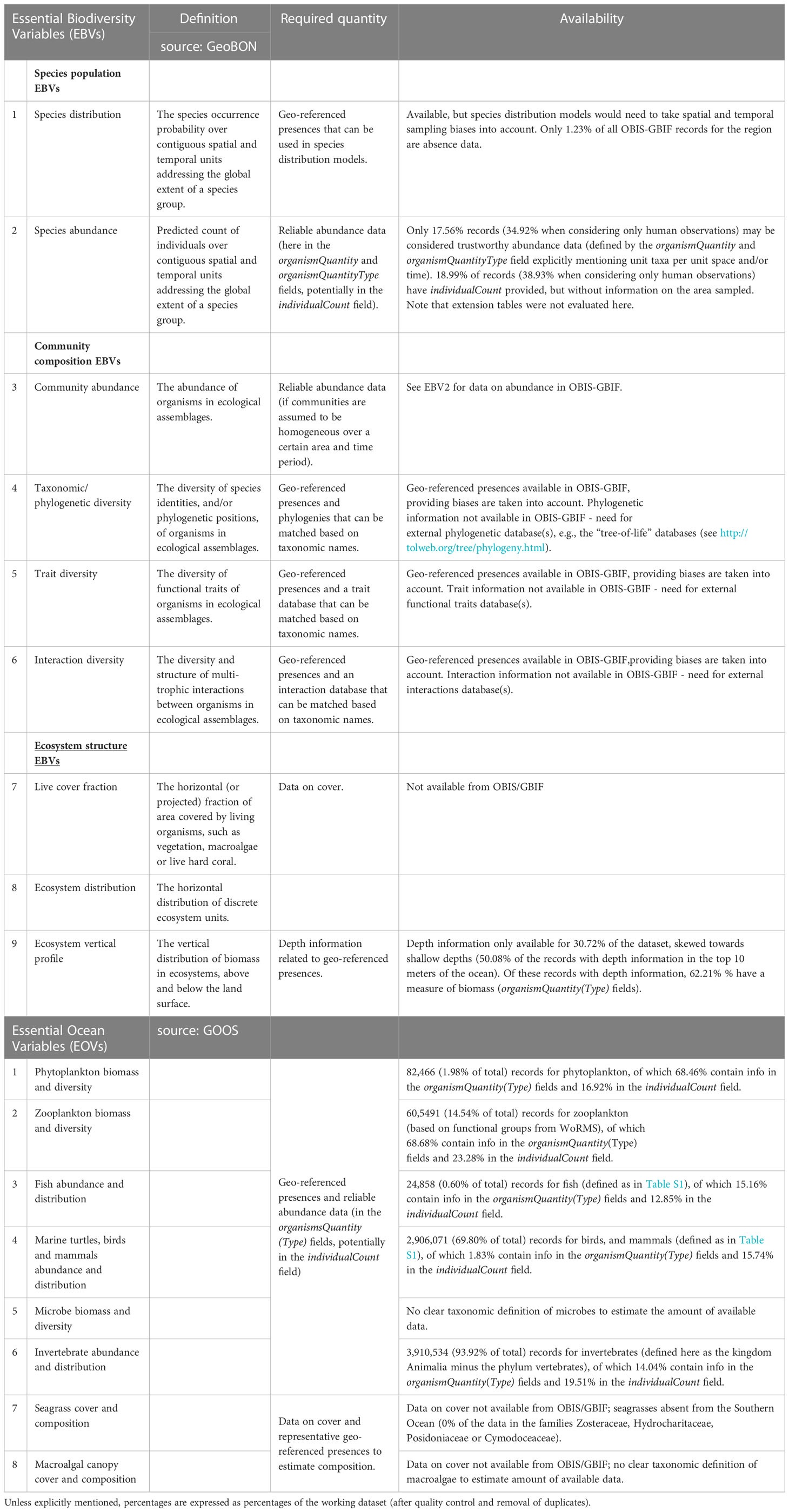
Table 1 List of Essential Biodiversity and Essential Ocean Variables, and the availability of suitable data in OBIS and GBIF to calculate them.

2.4 Suitability of the available data for a MEASO

Based on definitions provided by GEO BON and GOOS (see Table 1 for details), we identified, for each relevant EBV and EOV, the data necessary for their calculation. We then evaluated how appropriate data from OBIS and GBIF are for this exercise, based on qualitative evaluation of biases as well as quantitative evaluations of the percentage of records containing the required information. Note that our evaluation of the availability of abundance data was focused on the organismQuantity(Type) and individualCount columns, and excluded information that may have been recorded in extension tables (Extended Measurement or Fact), as only occurrence data was included in this analysis. This may underestimate to a certain extent the availability of abundance data.

2.5 Code availability

All analyses were performed in R-studio (R version 4.4.1; R Core Team, 2021). The R-code of the analyses has been extensively documented and is freely available at GitHub (https://github.com/asbonnetlebrun/measo_gap_analysis).

3 Results

3.1 Data availability and overall quality

The search criteria matched 5,993,533 records on OBIS and 5,579,904 on GBIF. Of these, 547,944 records appeared to be situated on land (Figure 1). In total, 1,478 records had no scientificName (0.01% of the data), and 467,966 records had a scientificName with no match in WoRMS (4.04% of the data). Note that for records from DNA sequence reads, the number without a scientificName match in WoRMS increased substantially to 40.56%.

FIGURE 1

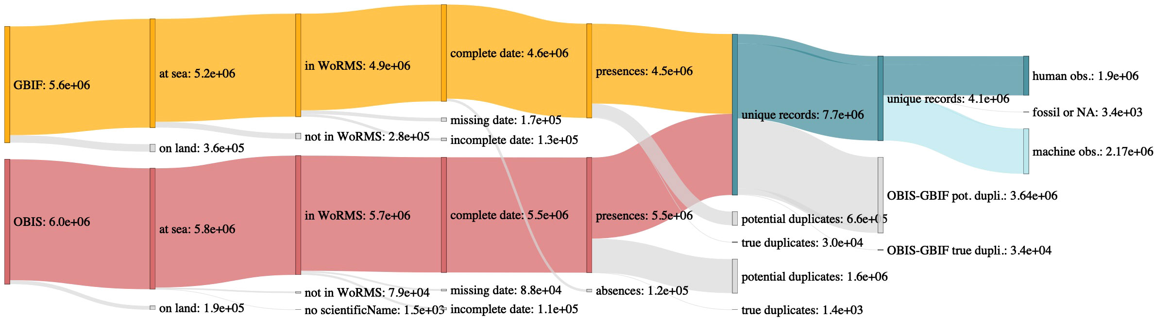
Figure 1 Sankey diagram of quality control steps: removing records on land, records with no match in WoRMS for their scientificName, records with incomplete or missing dates, absences, potential within-database duplicates, potential between-databases duplicates, and fossil records. Each category is followed by the number of records that fits in it. Orange: data from GBIF, red: data from OBIS, blue: unique records across the two combined databases, grey: discarded data.

5.04% of records had incomplete date information (year missing for 2.84% of records, month for 4.55% and day for 5.04%). In addition, 5,369 records prior to 1773 (first recorded crossing of the Antarctic circle), and 6 records after 2022, were flagged as erroneous for further removal (e.g. 5,353 records supposedly in year 0). 141,966 records (1.23% of all data) referred to species absences (all from GBIF; Figure 1).

7,002,899 (60.51% of the total) records were potential duplicates of other records (2,118,495 within OBIS, 1,373,050 within GBIF, and 3,511,354 between the two databases, leaving 4,570,538 unique records in the database. Machine observations accounted for 39.89% of all records (before quality controls), and human observations for 60.11%, with the remaining ~3400 records being unclassified or fossil records.

Only 19.39% of all (i.e., presence and absence) records contained information on the number of individuals observed (individualCount field), and 26.27% of all records contained abundance information (i.e., explicit mention of number of individuals per unit of space and/or time in the organismQuantity and organismQuantityType fields). Note that absence records could be considered as carrying abundance information (i.e., null abundance) but the individualCount and organismQuantity fields were filled in for respectively only 3.46% and 68.17% of absence records. An occurrenceID was missing for 953,954 records (8.24%), probably pre-dating the implementation of occurrenceID as an obligatory field.

Records originated from 3,484 individually identified datasets (based on unique value in the datasetName field) and 570 institutions (institutionCode field) - but note that 10,751,553 records had no data in the datasetName field and 5,582,236 records had no data in the institutionCode field. The contributions of individual datasets were highly variable: 2,929 datasets had less than 10 records, while 6 datasets had more than 50,000 records (including “The Retrospective Analysis of Antarctic Tracking (Standardised) Data from the Scientific Committee on Antarctic Research” and “Southern Ocean Continuous Zooplankton Recorder (SO-CPR) Survey”). Molecular data (“DNA sequence reads” in the organismQuantityType field, as recommended in Andersson et al., 2021) represented 2.76% of the whole dataset.

Only 54.88% of all records contained information in the samplingProtocol field. When present, information in this field was not always recorded in a standardised manner, resulting in 4,885 unique values in this field, making a systematic study of the impact of sampling protocols on spatial and temporal biases impractical.

3.2 Exploration of distributions and biases

All subsequent results will refer to the filtered dataset (no terrestrial records, presences only, unique records, complete and realistic dates, machine or human observations).

3.2.1 Temporal distribution

Most observations were collected during the 20th and 21st centuries (only 0.04% of records prior to 1900, 63.9% of which classified as preserved specimen), with an increase starting around the 1950s and a decrease in the last decade – for both machine and human observations (Figure 2A). There was also a consistent seasonal bias in the data, particularly for human observations, which showed higher sampling intensity during the austral summer months (Figure 2B). Note that the peak in human observations in May in the last decade is dominated by what seems to be one campaign collecting and analyzing environmental DNA (i.e., “DNA sequence reads” in the organismQuantityType column) in 2016 in the West Pacific MEASO sector (70.37% of the 2000-2019 May peak; Supplementary Figure 1A, B). Overall, molecular data only started to represent a significant amount of data in the last decade (2010-2019; Supplementary Figure 1A).

FIGURE 2

Figure 2 Temporal distribution of the data (after quality control): (A) number of records per year, along with some key expeditions (Discovery Investigations, Biological Investigations Of Marine Antarctic Systems and Stocks (BIOMASS) survey, Southern Ocean Continuous Plankton Recorder surveys (SO-CPR) and Census of Antarctic Marine Life (CAML); (B) number of records per month, separated into decades and human vs. machine observations.

3.2.2 Geographic distribution

Human observations were highly clustered (Figure 3A), with high record densities around Sub-Antarctic islands, and visible cruise tracks, e.g., between the Antarctic continent and New-Zealand or Australia. The number of human observation records per unit area was highest – and increased the most in recent years – in the Sub-Antarctic zone of the Central Indian sector, the Antarctic zone of the East Pacific sector, and the sub-Antarctic and Northern zones of the East Indian sector (Figure 4). High numbers of human observations were found around sub-Antarctic Islands, and along routes leading to research stations (Supplementary Figure 2A). In winter, human observations were almost absent from large areas covered by sea ice (Supplementary Figure 3), although areas in the Central Indian Ocean remained sampled in winter despite the presence of sea ice. In contrast, although most abundant around research stations (Antarctic Peninsula, sub-Antarctic islands, some areas on the Antarctic coast; Supplementary Figure 2B), machine observation data covered a larger part of the Southern Ocean and appeared not to be confounded by ship movement (Figure 3B, Supplementary Figures 2B, 4). However, in the case of tracking data from central-place foragers (a large part of the dataset), they will likely be biased by sampled colonies.

FIGURE 3

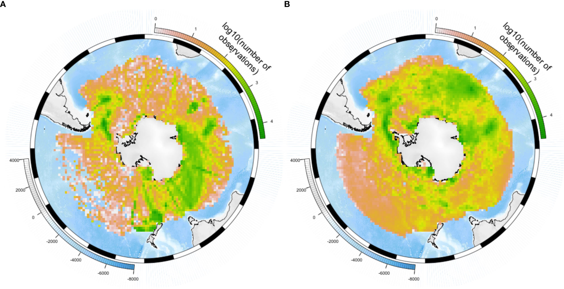
Figure 3 Geographic distribution of the number of records. (A) Human observations, (B) Machine observations.

FIGURE 4

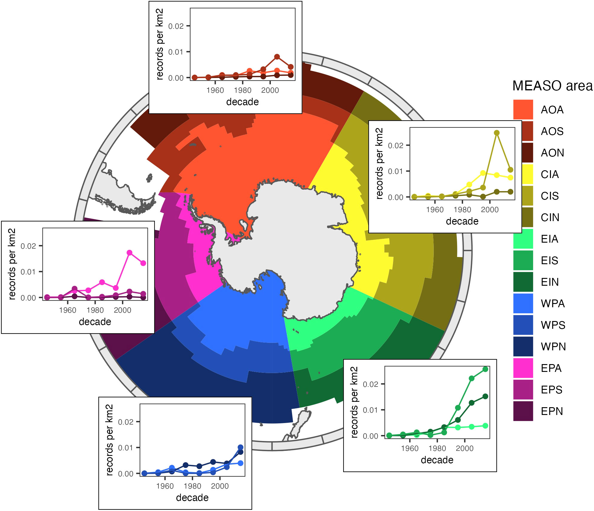
Figure 4 Number of human observations per km² per decade for each MEASO area. The MEASO areas divide the Southern Ocean into five longitudinal sectors: the West Pacific (WP), East Pacific (EP), Atlantic (AO), East Indian (EI), and Central Indian (CI). Each of these sectors is further subdivided into three longitudinal zones (from South to North): Antarctic (WPA, EPA, AOA, EIA and CIA), Sub-Antarctic (WPS, EPS, AOS, EIS and CIS), and Northern (WPN, EPN, AON, EIN and CIN).

3.2.3 Taxonomic composition

Overall, the data included 23,947 different taxonomic units, based on values from the scientificName field, after matching with the WoRMS taxonomic backbone. These units ranged from (sub-)species to kingdom-level identifications. After matching with the WoRMS taxonomic backbone, we identified 93 individual phyla in the data. The 10 best represented phyla for the whole working dataset (machine and human observations) were Chordata (3,146,356 records), Arthropoda (506,936), Mollusca (70,372), Echinodermata (66,693), Foraminifera (57,147), Ochrophyta (56,567), Cnidaria (36,977), Proteobacteria (28,092), Bryozoa (25,822), and Annelida (25,512). The evolution of the number of records through time varied across phyla, with several phyla increasing until 2001-2010 and then plateauing or decreasing in the last decade, while Proteobacteria, which were absent from the databases until the decade 1980-1989, showing a very marked increase continuing in the last decade, making them to the 3rd currently most-sampled phylum (Supplementary Figure 5).

The depth of taxonomic identification varied with observation types: while 99.95% of machine observations were identified at the genus level, and 99.93% at the species level, only 83.96% of human observations were identified at the genus level, and only 70.48% at the species level. The depth of taxonomic identification also varied among phyla, with large and morphologically easily identifiable phyla such as Chordata (but also Mollusca, up to genus level) identified more precisely than phyla such as Radiozoa, Chaetognatha, Foraminifera and Proteobacteria (Supplementary Figure 6), those phyla often requiring microscopy to reach fine level identifications or DNA-based techniques, which often identify currently undescribed taxonomic units (Andersson et al., 2021). As an illustration of this, only 6.99% of molecular data were identified at the species level.

86.3% of filtered records could be unambiguously matched to benthic/pelagic categories. Overall, pelagic species appeared better sampled than benthic species, with a higher number of records and higher spatial coverage (Figure 5). There were large disparities in the number of human observations covering each focal group (Figure 5A), as well as in the spatial coverage of each group (Figure 5B). Birds and mammals were by far the most sampled group, followed by Crustacea. Birds and mammals, and Crustacea were also the groups with the best spatial coverage. However, some groups had relatively low sampling but relatively good coverage (e.g., Mollusca, Gelatinous zooplankton, or Annelida). No group had a spatial coverage higher than 65%. Both the distribution of records among groups and spatial coverage also varied across MEASO areas (Supplementary Figures 7, 8). In addition, when considering molecular data only, the four dominant phyla were all micro-organisms (by order of data quantity: bacteria, microzooheterotrophs, eukaryote primary producers, and protozoa; Supplementary Figure 1C).

FIGURE 5

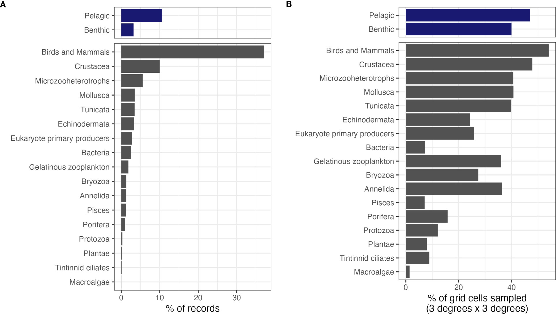
Figure 5 Data and spatial coverage for a range of focal groups, for human observations only. (A) Percentage of records belonging to each focal group; (B) for each focal group, percentage of cells of a 3° x 3° grid covering the MEASO area with at least one record.

In most sectors, no plateau was reached in the genus accumulation curves (Supplementary Figures 9-11), and even in the sector where a plateau was reached, there were very few cells that appeared to be sampled enough. In addition, the fit was poor for most sectors.

3.3 Suitability of the available data for a MEASO

Table 1 shows, for each relevant EBV or EOV, the data required for its calculation, and the fit for purpose of OBIS and GBIF data. In general, geo-referenced data are available for a range of taxa but (as discussed below) their suitability for a MEASO is hindered by the spatial, temporal, and taxonomic biases identified above. For variables that require abundance, biomass, trait, or depth data, large proportions of records do not contain suitable information.

4 Discussion

By exploring the temporal, spatial and taxonomic distributions of open biodiversity data in the SO, we found a strong seasonal and spatial bias, as well as an unbalanced representation of the different taxa. These limitations, along with limited information on certain variables of interest (e.g., absences, abundance, depth) might constrain the utility of such data for a MEASO. We also found consistent differences between human and machine observations, highlighting the need to treat these two data types separately when using these to calculate EBVs or EOVs.

4.1 Opportunities arising from open biodiversity databases for a MEASO

By providing enormous amounts of geo-referenced data (millions of records), on a large taxonomic diversity (thousands of taxonomic units) and with large spatial extent, OBIS and GBIF represent promising data infrastructures for mapping distributions in the Southern Ocean. These data aggregators are continuously growing, due to increased data collection and incentives to submit data to publicly accessible repositories, while standards for publishing these data are also constantly improving (Van de Putte et al., 2021). Several key expeditions and joint efforts can be related to periods with increased data collection visible in Figure 2 – e.g., the Discovery Investigations (1924-1951), the Biological Investigations Of Marine Antarctic Systems and Stocks (BIOMASS) survey (1980-1985), the Southern Ocean Continuous Plankton Recorder surveys (SO-CPR, 1991-), or the Census of Antarctic Marine Life (2005-2010) (see Griffiths, 2010 for a more detailed perspective). The rate of data accumulation has also increased drastically until the last decade – probably due to a delay between data collection and publication, and increased interest in certain (until recently under-sampled) taxa, suggesting that the utility of the database could keep increasing. This delay is often caused by the fact that samples need to be collected in the field, transported to a research institute and identified by experts who may only have limited time and resources. Here machine based observation can help close this temporal gap between observation and publication of data. Guidance on how to implement this exists for DNA derived data, GPS data (van der Kolk et al., 2022) and imaging devices (Mortelmans et al., 2019)

4.2 Challenges with using open biodiversity databases for a MEASO

However, the strong biases we highlighted in the data, severely limit their direct and widespread use for a MEASO. First, the data (particularly human observations) were strongly seasonally biased, because of sea-ice and prolonged darkness in the winter, complicating accessibility and work in the Southern Ocean. Second, the data were strongly biased towards certain regularly sampled sectors of the ocean. Most concerning is the spatial bias in human observations, with more data in recurrently visited areas – mostly around research stations of the Antarctic Peninsula and sub-Antarctic Islands, and along routes between other continents and these stations. Note that the environmental and socio-economic drivers of spatial sampling bias differ between the Southern Ocean and other systems [with the importance of, e.g., proximity to settlements or to well-funded research institutions (Meyer et al., 2016; Ramírez et al., 2022)]. But care also needs to be taken with machine observations, because of potentially stronger spatial autocorrelation in data such as animal tracking data (e.g., GPS), potential limitations in the types of taxa that can be observed by machine methods (e.g. tracking tags can only be deployed on certain animals), and other biases that might differ from those affecting human observations. Third, there was a strong imbalance in the representation of different taxa, with birds and mammals largely dominating the database, followed by other widespread and conspicuous taxa [e.g., Crustacea, as in (Ramírez et al., 2022)]. This taxonomic bias is also evolving, with certain taxa becoming comparatively increasingly sampled – e.g., some microbes, due to developing technologies. Finally, missing relevant information – such as limited records of absences, or missing abundance or depth information for many records – can also strongly limit the utility of such data for a MEASO.

4.3 Recommendations for using open biodiversity databases for a MEASO

There are two avenues for enhancing the utility of open biodiversity databases for a MEASO: (1) improvements in the available data, and (2) corrections for the above-mentioned biases by using appropriate models.

As mentioned above, there is a strong need for additional data in under-sampled areas (e.g., in the Pacific), in the winter, and for less charismatic and smaller taxa. This can be achieved both by data collection and data mobilization. Indeed, if we strongly encourage data collection programs to fill in the gaps, we must be conscious of the costs involved in collecting and publishing those data. To complement new collection activities, there are existing data that are not yet in GBIF or OBIS – either because they have not yet been made publicly available, or because they have been submitted to other (often more local) databases not linked to GBIF or OBIS. Encouragements to publish data in public databases linked to GBIF or OBIS (possibly extending existing requirements by funding agencies to make data openly available) should be reinforced, and particularly target those key missing taxa, areas, and season. Some data types, e.g., molecular data or data from autonomous observation devices, are becoming more and more important and allow access to under sampled organisms or areas. However, these data are currently found only in limited amounts in GBIF and OBIS, while geospatial information is often missing in the databases in which they are published (e.g., consistently low percentage of georeferenced data on NCBI GenBank, Gratton et al., 2017). Encouraging linking between databases, following good practices (including efforts to address shortcomings related to taxonomic reliability and lack of standardized metadata vocabulary; Andersson et al., 2021), would enhance their discovery and use in a spatial context. In general, making more data available through GBIF and OBIS, the most widely used biodiversity research data infrastructures in the Southern Ocean would comply with the FAIR principles (Wilkinson et al., 2016), which aim to increase the Findability, Accessibility, Interoperability and Reusability of digital datasets. Indeed, the two portals are recognized as the key repositories by many international instances – e.g. the Intergovernmental Science-Policy Platform on Biodiversity and Ecosystem Services (IPBES; see https://assets.ctfassets.net/uo17ejk9rkwj/6ddNMnbw7CiSIkusowkS4e/f5fd21478e21f984b6276709eca31b3b/IPBES_memorandum.pdf, https://www.ipbes.net/sites/default/files/factsheet_gbif_growth_in_species_occurrence_records.pdf), the Convention on Biological Diversity (CBD), or the International Panel for Climate Change (IPCC; see Johnson et al., 2023) – and follow common data standards (DwC standards). Finally, encouragement by data aggregators to fill in certain fields that are not currently mandatory (e.g., fields related to abundance or depth) or to also publish absence records (to provide information on the distribution of sampling effort) could increase the utility of the data.

The collection and mobilization of additional data is a process that takes time and money. Modelling techniques cannot replace primary data collection, but might provide complementary approaches that can go some way towards correcting for biases – particularly spatial biases. Modelling is a potential avenue for obtaining improved information and derived products such as species distributions, both in the shorter term as more data is collected but also as a means of maximizing the value of larger data collections. However, there are multiple precautionary steps to correctly apply species distribution models (SDMs) to these data. First, data should be rigorously quality controlled before any application. This involves basic quality control steps as those carried out in this study, but should ideally be more thorough, and more specific to the study taxa, involving experts to remove other potentially erroneous records (e.g., likely misidentifications, errors in coordinates). This was done for example in the Biogeographic Atlas of the Southern Ocean ( de Broyer and Koubbi, 2014). Second, caution should be taken when extrapolating results to environmental conditions absent from the data (Guillaumot et al., 2020), which is likely to occur across such large scales considering the large gaps in the data. Additionally, and most importantly, there are a whole range of modelling difficulties that can impact model performance. An obvious example of this is spatial sampling bias (Beck et al., 2014; Pender et al., 2019). Correcting for sampling bias in species distribution models requires some layer representing sampling effort, used for example to guide the selection of background locations (Guillaumot et al., 2021) or as a control variable (e.g., Warton et al., 2013). Contrary to certain cases where sampling completeness can be known (e.g., when there is some reference of species ranges, e.g. Meyer et al., 2015, 2016), in other cases it must be estimated or modelled (e.g., as a function of other spatial variables (Zizka et al., 2021), or based on records of similar species – sampled with similar protocols (Guillaumot et al., 2019)). Other forms of sampling bias can be introduced when combining datasets collected with different survey designs, sampling protocols or gear (e.g. human vs. machine observations, or different net types and sizes), recording methodology (e.g. presence-only, presence-absence, abundance), seasonal timing, or other factors. Some information about these factors may be provided in the aggregated records, for example in the samplingProtocol field. However, as noted above, we found this field to be inconsistently populated and with varying terminology. Adoption of stricter requirements in this field might improve this situation. However, bias correction is an active field of research and methods can be non-trivial (Renner et al., 2019; Matthiopoulos et al., 2022). While the Darwin Core standard has the capability to include the detailed metadata that would be necessary to support these kinds of advanced analyses, it is perhaps impractical to expect such a degree of metadata to be consistently populated in large, aggregated data infrastructures like GBIF and OBIS. However, even for such specialized applications, these data infrastructures provide a valuable service by indexing available datasets that might be provided in other, more detailed forms elsewhere, including as primary data from the author’s institutional data repository. Data collected specifically for MEASO activities might reasonably be published through multiple data networks (e.g. as in Andrews-Goff et al., 2022), and this can potentially be done using dedicated packages, e.g., movepub package (Desmet, 2023) to publish data from Movebank (movebank.org) to GBIF. The above-mentioned modelling difficulties inherent to biased data, along with others that go beyond the scope of this discussion, need to be carefully considered (for more recommendations on applying SDMs to data from global open biodiversity databases, see for example Anderson et al., 2016) and highlight the fact that modelling should not be considered as a replacement for more primary data collection.

In conclusion, although open biodiversity databases offer promises for MEASOs, care must be taken when using these data because of their inherent spatial, temporal, and taxonomic biases. There is a considerable need for additional data in under-sampled regions, in the winter, and for less conspicuous taxa, as well as reliable abundance or depth data, along with improvements in modelling techniques that can better account for the biases and limitations of Southern Ocean marine biodiversity data and thereby support balanced and informative ecosystem assessments.

Data availability statement

Publicly available datasets were analyzed in this study. This data can be found here: Data are available from OBIS (https://obis.org) and GBIF (http://www.gbif.org, https://doi.org/10.15468/dl.8w7bux). Codes to clean and analyze the data are available at https://github.com/asbonnetlebrun/measo_gap_analysis.

Ethics statement

There are no ethical considerations for this work, which entirely re-uses openly available data collected for other purposes.

Author contributions

A-SB-L analyzed the data and led the writing of the manuscript. MaS, PP, MiS, AV, and BR assisted with analysis. YR-C and AV provided overall supervision. All authors contributed to the article and approved the submitted version.

Funding

A-SB-L was funded by a grant from the Antarctic and Southern Ocean Coalition – grant number OPE-2021-0507, the French French Biodiversity Agency (OFB) and the French Ministry of Ecological Transition and Territorial Cohesion. AV and MaS were funded by the Belgian Science Policy Office (BELSPO, contract n°FR/36/AN1/AntaBIS) in the Framework of EU-Lifewatch. In addition, AV was funded through the FED-tWIN grant Prf-2019-005_SO-BOMP. HG was funded by the British Antarctic Survey and NERC.

Acknowledgments

This work was a core contribution to the first Marine Ecosystem Assessment for the Southern Ocean (MEASO) of IMBeR’s program ICED. We thank the MEASO Support Group and Steering Committee for their assistance during the various stages of the MEASO development process. We also thank the three reviewers for their constructive comments and suggestions that helped improve the document.

Conflict of interest

The authors declare that the research was conducted in the absence of any commercial or financial relationships that could be construed as a potential conflict of interest.

The handling editor JM-T declared a shared committee with authors HG and AV at the time of review.

Publisher’s note

All claims expressed in this article are solely those of the authors and do not necessarily represent those of their affiliated organizations, or those of the publisher, the editors and the reviewers. Any product that may be evaluated in this article, or claim that may be made by its manufacturer, is not guaranteed or endorsed by the publisher.

Supplementary material

The Supplementary Material for this article can be found online at: https://www.frontiersin.org/articles/10.3389/fmars.2023.1150603/full#supplementary-material

References

Anderson R. P., Araújo M., Guisan A., Lobo J. M., Martínez-Meyer E. (2016). Are species occurrence data in global online repositories fit for modeling species distributions? Case Global Biodiversity Inf. Facility (GBIF) 27.

Google Scholar

Andersson A. F., Bissett A., Finstad A. G., Fossøy F., Grosjean M., Hope M., et al. (2021). Publishing DNA-derived data through biodiversity data platforms (Copenhaguen: GBIF Secretariat). doi: 10.35035/doc-vf1anr22

CrossRef Full Text | Google Scholar

Andrews-Goff V., Bell E., Miller B., Wotherspoon S., Double M. (2022). Satellite tag derived data from two Antarctic blue whales (Balaenoptera musculus intermedia) tagged in the east Antarctic sector of the southern ocean. Biodiversity Data J. 10, e94228. doi: 10.3897/BDJ.10.e94228

CrossRef Full Text | Google Scholar

Beck J., Böller M., Erhardt A., Schwanghart W. (2014). Spatial bias in the GBIF database and its effect on modeling species’ geographic distributions. Ecol. Inf. 19, 10–15. doi: 10.1016/j.ecoinf.2013.11.002

CrossRef Full Text | Google Scholar

Brasier M. J., Barnes D., Bax N., Brandt A., Christianson A. B., Constable A. J., et al. (2021). Responses of southern ocean seafloor habitats and communities to global and local drivers of change. Front. Mar. Sci. 8. doi: 10.3389/fmars.2021.622721

CrossRef Full Text | Google Scholar

Brasier M. J., Constable A., Melbourne-Thomas J., Trebilco R., Griffiths H., Van de Putte A., et al. (2019). Observations and models to support the first marine ecosystem assessment for the southern ocean (MEASO). J. Mar. Syst. 197, 103182. doi: 10.1016/j.jmarsys.2019.05.008

CrossRef Full Text | Google Scholar

de Broyer C., Koubbi P. (2014). Biogeographic atlas of the Southern Ocean. De Broyer C., Koubbi P., Griffiths H. J., Raymond B., Udekem d’Acoz C. d’., Van de Putte A. P., Danis B., David B., Grant S., Gutt J., Held C., Hosie G., Huettmann F., Post A., Ropert-Coudert Y. (eds.). (Cambridge:SCAR) 510.

Google Scholar

Caccavo J. A., Christiansen H., Constable A. J., Ghigliotti L., Trebilco R., Brooks C. M., et al. (2021). Productivity and change in fish and squid in the southern ocean. Front. Ecol. Evol. 9. doi: 10.3389/fevo.2021.624918

CrossRef Full Text | Google Scholar

Chamberlain S. (2020) Worrms: world register of marine species (WoRMS) client. r package version 0.4.2. Available at: https://CRAN.R-project.org/package=worrms.

Google Scholar

Chamberlain S., Oldoni D., Barve V., Desmet P., Geffert L., Mcglinn D., et al. (2023) Rgbif: interface to the global 'Biodiversity' information facility 'API'. r package version 3.7.5. Available at: https://CRAN.R-project.org/package=rgbif.

Google Scholar

Constable A. J., Costa D. P., Schofield O., Newman L., Urban E. R., Fulton E. A., et al. (2016). Developing priority variables (“ecosystem essential ocean variables” {{/amp]]mdash; eEOVs) for observing dynamics and change in southern ocean ecosystems. J. Mar. Syst. 161, 26–41. doi: 10.1016/j.jmarsys.2016.05.003

CrossRef Full Text | Google Scholar

De Pooter D., Appeltans W., Bailly N., Bristol S., Deneudt K., Eliezer M., et al. (2017). Toward a new data standard for combined marine biological and environmental datasets - expanding OBIS beyond species occurrences. Biodiversity Data J., e10989. doi: 10.3897/BDJ.5.e10989

CrossRef Full Text | Google Scholar

Desmet P. (2023) Movepub: prepare movebank data for publication. r package version 0.1.0. Available at: https://github.com/inbo/movepub.

Google Scholar

GBIF.org (2022) GBIF occurrence. doi: 10.15468/dl.8w7bux.

CrossRef Full Text | Google Scholar

Grant S. M., Hill S. L., Trathan P. N., Murphy E. J. (2013). Ecosystem services of the southern ocean: trade-offs in decision-making. Antarctic Sci. 25, 603–617. doi: 10.1017/S0954102013000308

CrossRef Full Text | Google Scholar

Grant S. M., Waller C. L., Morley S. A., Barnes D. K. A., Brasier M. J., Double M. C., et al. (2021). Local drivers of change in southern ocean ecosystems: human activities and policy implications. Front. Ecol. Evol. 9. doi: 10.3389/fevo.2021.624518

CrossRef Full Text | Google Scholar

Gratton P., Marta S., Bocksberger G., Winter M., Trucchi E., Kühl H. (2017). A world of sequences: can we use georeferenced nucleotide databases for a robust automated phylogeography? J. Biogeogr. 44, 475–486. doi: 10.1111/jbi.12786

CrossRef Full Text | Google Scholar

Griffiths H. J. (2010). Antarctic Marine biodiversity – what do we know about the distribution of life in the southern ocean? PloS One 5, e11683. doi: 10.1371/journal.pone.0011683

PubMed Abstract | CrossRef Full Text | Google Scholar

Griffiths H. J., Van de Putte A. P., Danis B. (2014). “Chapter 2.2. data distribution: patterns and implications,” in Biogeographic atlas of the southern ocean. Eds. Broyer C., Koubbi P., Griffiths H. J., Raymond B., d’Udekem d’Acoz C.. (The Scientific Committee on Antarctic Research, Scott Polar Research Institute Cambridge), 16–26.

Google Scholar

Guillaumot C., Artois J., Saucède T., Demoustier L., Moreau C., Eléaume M., et al. (2019). Broad-scale species distribution models applied to data-poor areas. Prog. Oceanogr. 175, 198–207. doi: 10.1016/j.pocean.2019.04.007

CrossRef Full Text | Google Scholar

Guillaumot C., Danis B., Saucède T. (2021). Species distribution modelling of the southern ocean benthos: a review on methods, cautions and solutions. Antarctic Sci. 33 (4), 349–372. doi: 10.1017/S0954102021000183

CrossRef Full Text | Google Scholar

Guillaumot C., Moreau C., Danis B., Saucède T. (2020). Extrapolation in species distribution modelling. application to southern ocean marine species. Prog. Oceanogr. 188, 102438. doi: 10.1016/j.pocean.2020.102438

CrossRef Full Text | Google Scholar

Henley S. F., Cavan E. L., Fawcett S. E., Kerr R., Monteiro T., Sherrell R. M., et al. (2020). Changing biogeochemistry of the southern ocean and its ecosystem implications. Front. Mar. Sci. 7. doi: 10.3389/fmars.2020.00581

CrossRef Full Text | Google Scholar

Jetz W., McGeoch M. A., Guralnick R., Ferrier S., Beck J., Costello M. J., et al. (2019). Essential biodiversity variables for mapping and monitoring species populations. Nat. Ecol. Evol. 3, 539–551. doi: 10.1038/s41559-019-0826-1

PubMed Abstract | CrossRef Full Text | Google Scholar

Johnson K. R., Owens I. F. P., The Global Collection Group (2023). A global approach for natural history museum collections. Science 379, 1192–1194. doi: 10.1126/science.adf6434

PubMed Abstract | CrossRef Full Text | Google Scholar

Kennicutt M. C., Chown S. L., Cassano J. J., Liggett D., Massom R., Peck L. S., et al. (2014). Polar research: six priorities for Antarctic science. Nature 512, 23–25. doi: 10.1038/512023a

PubMed Abstract | CrossRef Full Text | Google Scholar

Matthiopoulos J., Wakefield E., Jeglinski J. W. E., Furness R. W., Trinder M., Tyler G., et al. (2022). Integrated modelling of seabird-habitat associations from multi-platform data: a review. J. Appl. Ecol. 59, 909–920. doi: 10.1111/1365-2664.14114

CrossRef Full Text | Google Scholar

Meyer C., Jetz W., Guralnick R. P., Fritz S. A., Kreft H. (2016). Range geometry and socio-economics dominate species-level biases in occurrence information. Global Ecol. Biogeogr. 25, 1181–1193. doi: 10.1111/geb.12483

CrossRef Full Text | Google Scholar

Meyer C., Weigelt P., Kreft H. (2015). Multidimensional biases, gaps and uncertainties in global plant occurrence information. PeerJ. PrePrints 6, 8221. doi: 10.7287/peerj.preprints.1326v2

CrossRef Full Text | Google Scholar

Miloslavich P., Bax N. J., Simmons S. E., Klein E., Appeltans W., Aburto-Oropeza O., et al. (2018). Essential ocean variables for global sustained observations of biodiversity and ecosystem changes. Global Change Biol. 24, 2416–2433. doi: 10.1111/gcb.14108

CrossRef Full Text | Google Scholar

Morley S. A., Abele D., Barnes D. K. A., Cárdenas C. A., Cotté C., Gutt J., et al. (2020). Global drivers on southern ocean ecosystems: changing physical environments and anthropogenic pressures in an earth system. Front. Mar. Sci. 7. doi: 10.3389/fmars.2020.547188

CrossRef Full Text | Google Scholar

Mortelmans J., Goossens J., Amadei Martínez L., Deneudt K., Cattrijsse A., Hernandez F. (2019). LifeWatch observatory data: zooplankton observations in the Belgian part of the north Sea. Geosci. Data J. 6, 76–84. doi: 10.1002/gdj3.68

CrossRef Full Text | Google Scholar

Moudrý V., Devillers R. (2020). Quality and usability challenges of global marine biodiversity databases: an example for marine mammal data. Ecol. Inf. 56, 101051. doi: 10.1016/j.ecoinf.2020.101051

CrossRef Full Text | Google Scholar

Muller-Karger F. E., Miloslavich P., Bax N. J., Simmons S., Costello M. J., Sousa Pinto I., et al. (2018). Advancing marine biological observations and data requirements of the complementary essential ocean variables (EOVs) and essential biodiversity variables (EBVs) frameworks. Front. Mar. Sci. 5. doi: 10.3389/fmars.2018.00211

CrossRef Full Text | Google Scholar

Nilsson R. H., Andersson A. F., Bissett A., Finstad A. G., Fossøy F., Grosjean M., et al. (2022). Introducing guidelines for publishing DNA-derived occurrence data through biodiversity data platforms. Metabarcoding Metagenomics 6, e84960. doi: 10.3897/mbmg.6.84960

CrossRef Full Text | Google Scholar

Pender J. E., Hipp A. L., Hahn M., Kartesz J., Nishino M., Starr J. R. (2019). How sensitive are climatic niche inferences to distribution data sampling? a comparison of biota of north America program (BONAP) and global biodiversity information facility (GBIF) datasets. Ecol. Inf. 54, 100991. doi: 10.1016/j.ecoinf.2019.100991

CrossRef Full Text | Google Scholar

Pereira H. M., Ferrier S., Walters M., Geller G. N., Jongman R. H. G., Scholes R. J., et al. (2013). Essential biodiversity variables. Science 339, 277–278. doi: 10.1126/science.1229931

PubMed Abstract | CrossRef Full Text | Google Scholar

Petrou K., Baker K. G., Nielsen D. A., Hancock A. M., Schulz K. G., Davidson A. T. (2019). Acidification diminishes diatom silica production in the southern ocean. Nat. Clim. Change 9, 781–786. doi: 10.1038/s41558-019-0557-y

CrossRef Full Text | Google Scholar

Provoost P., Bosch S. (2021). robis: ocean biodiversity information system (OBIS) Client. R package version 2.8.2 Available at: https://CRAN.R-project.org/package=robis.

Google Scholar

R Core Team (2021). R: A language and environment for statistical computing (Vienna, Austria: R Foundation for Statistical Computing). Available at: https://www.R-project.org/.

Google Scholar

Ramírez F., Sbragaglia V., Soacha K., Coll M., Piera J. (2022). Challenges for marine ecological assessments: completeness of findable, accessible, interoperable, and reusable biodiversity data in European seas. Front. Mar. Sci. 8. doi: 10.3389/fmars.2021.802235

CrossRef Full Text | Google Scholar

Renner I. W., Louvrier J., Gimenez O. (2019). Combining multiple data sources in species distribution models while accounting for spatial dependence and overfitting with combined penalized likelihood maximization. Methods Ecol. Evol. 10, 2118–2128. doi: 10.1111/2041-210X.13297

CrossRef Full Text | Google Scholar

Rogers A. D., Frinault B. A. V., Barnes D. K. A., Bindoff N. L., Downie R., Ducklow H. W., et al. (2020). Antarctic Futures: an assessment of climate-driven changes in ecosystem structure, function, and service provisioning in the southern ocean. Annu. Rev. Mar. Sci. 12, 87–120. doi: 10.1146/annurev-marine-010419-011028

CrossRef Full Text | Google Scholar

Schiaparelli S., Danis B., Wadley V., Michael Stoddart D. (2013). “The census of Antarctic marine life: the first available baseline for Antarctic marine biodiversity,” in Adaptation and evolution in marine environments, vol. 2 . Eds. Verde C., di Prisco G. (Berlin, Heidelberg: Springer Berlin Heidelberg), 3–19. From Pole to Pole. doi: 10.1007/978-3-642-27349-0_1

CrossRef Full Text | Google Scholar

Sumner M. D. (2020) Measoshapes: southern ocean shapes for “MEASO” work. r package version 0.0.05.2. Available at: https://github.com/AustralianAntarcticDivision/measoshapes.

Google Scholar

Vandepitte L., Bosch S., Tyberghein L., Waumans F., Vanhoorne B., Hernandez F., et al. (2015). Fishing for data and sorting the catch: assessing the data quality, completeness and fitness for use of data in marine biogeographic databases. Database 2015, bau125. doi: 10.1093/database/bau125

PubMed Abstract | CrossRef Full Text | Google Scholar

Van de Putte A. P., Griffiths H. J., Brooks C., Bricher P., Sweetlove M., Halfter S., et al. (2021). From data to marine ecosystem assessments of the southern ocean: achievements, challenges, and lessons for the future. Front. Mar. Sci. 8. doi: 10.3389/fmars.2021.637063

CrossRef Full Text | Google Scholar

van der Kolk H.-J., Desmet P., Oosterbeek K., Allen A. M., Baptist M. J., Bom R. A., et al. (2022). GPS Tracking data of Eurasian oystercatchers (Haematopus ostralegus) from the Netherlands and Belgium. ZooKeys 1123, 31–45. doi: 10.3897/zookeys.1123.90623

PubMed Abstract | CrossRef Full Text | Google Scholar

Warton D. I., Renner I. W., Ramp D. (2013). Model-based control of observer bias for the analysis of presence-only data in ecology. PloS One 8, e79168. doi: 10.1371/journal.pone.0079168

PubMed Abstract | CrossRef Full Text | Google Scholar

Wieczorek J., Bloom D., Guralnick R., Blum S., Döring M., Giovanni R., et al. (2012). Darwin Core: an evolving community-developed biodiversity data standard. PloS One 7, e29715. doi: 10.1371/journal.pone.0029715

PubMed Abstract | CrossRef Full Text | Google Scholar

Wilkinson M. D., Dumontier M., Aalbersberg I., Appleton G., Axton M., Baak A., et al. (2016). The FAIR guiding principles for scientific data management and stewardship. Sci. Data 3, 160018. doi: 10.1038/sdata.2016.18

PubMed Abstract | CrossRef Full Text | Google Scholar

Zizka A., Antonelli A., Silvestro D. (2021). Sampbias, a method for quantifying geographic sampling biases in species distribution data. Ecography 44, 25–32. doi: 10.1111/ecog.05102

CrossRef Full Text | Google Scholar