Longitudinal and lateral circulation and tidal impacts in salt-plug estuaries

1 Introduction

A salt plug or salinity maximum zone can form in an estuary when evaporation rates compare to river discharge (Valle-Levinson, 2010). If we have on one side the river and on the other side a salty ocean, it is normal to expect that, in the estuary, salinity will continuously decrease from the mouth to the head. A situation in which a salt plug forms is if evaporative losses are such that they do not add salt but extract fresh water from the estuary. A small river runoff can overcome the evaporation only close to the head of the estuary. This area thus develops typical gravitational circulation. The high evaporation results in waters that are saltier than waters in the open ocean with a maximum salinity zone. A salt plug separates positive gravitational circulation, landward of the salt plug, from inverse gravitational circulation seaward of the salt plug. An example of a salt-plug estuary was first given by Wolanski (1986) for the Alligator River Estuary in northern Australia. Other similar highly evaporative systems are the Gulf of Fonseca on the Pacific side of Central America (Valle‐Levinson and Bosley, 2003), the bay of Malampaya Sound in Palawan in the Philippines (Cabrera et al., 2014), the Pasur River Estuary in southern Bangladesh (Shaha and Cho, 2016), and the Mond River Estuary on the northern coast of the Persian Gulf during summer (Ghaemi and Gholamipour, 2017). The latter belongs to the type of low-inflow estuaries in the category of “arid coasts” (Largier, 2010; Hosseini and Siadatmousavi, 2018). However, a salt plug can also form in typical positive estuaries without arid conditions, such as Barataria Bay, and in the Mississippi River Delta, in which freshwater pulses from the ocean into the bay may develop a salinity maximum zone (Juarez et al., 2020).

In estuaries, secondary (lateral) currents are perpendicular and up to 10% of the magnitude of axial flows (Rozovskii, 1957; Geyer, 1993; Chant, 2010). Despite its relatively small magnitude, secondary circulation greatly impacts estuarine dispersion (Chant, 2010). Li et al. (2014) specified at least four important mechanisms that drive lateral circulation in positive straight estuaries: (1) differential advection of along-channel or longitudinal density (salinity) gradients (Nunes and Simpson, 1985, Lerczak and Geyer, 2004, Li et al., 2014), (2) cross-channel variation in mixing (Chant, 2010) or boundary mixing on a sloping bottom (Phillips, 1970; Wunsch, 1970; Chen and Sanford, 2009; Li et al., 2014), (3) Ekman forcing (Johnson and Ohlsen, 1994; Ott and Garrett, 1998; Scully et al., 2009; Chant, 2010; Huijts et al., 2011; Li et al., 2014), and (4) interactions between barotropic tides and lateral variations in bathymetry(Li and O’Donnell, 1997; Li and Valle-Levinson, 1999; Khosravi et al., 2018). In curved channels, centrifugal accelerations represent a fifth mechanism for secondary circulation (Chant, 2010; Pein et al., 2018; Kranenburg et al., 2019).

In the absence of Coriolis acceleration and channel curvature, differential advection in positive estuaries is considered the main mechanism driving estuarine secondary flows (Chant, 2010). The analysis of differential advection of longitudinal salinity gradients is of utmost relevance in this study. Following Chant (2010) and considering only mechanisms that can generate the lateral salinity gradients associated with secondary circulations, the tendency (the time rate of change) of lateral salinity gradients ($\frac{\partial }{\partial t}\frac{\partial s}{\partial y}$) can be approximated as

$\begin{array}{ll}\frac{\partial }{\partial t}\frac{\partial s}{\partial y}=-\frac{\partial u}{\partial y}\frac{\partial s}{\partial x}-\frac{\partial w}{\partial y}\frac{\partial s}{\partial z}+\frac{\partial }{\partial y}\frac{\partial }{\partial z}(K_v\frac{\partial s}{\partial z})& (1)\end{array}$

where $s$ and $t$ are salinity and time, respectively, $y$ is the lateral (cross-channel) direction, $u$ and $w$ are the along-channel or longitudinal ($x$) and vertical ($z$) flows, respectively, and $K_v$ is the vertical eddy diffusivity of salt. The first term on the right-hand side of equation (1) describes the mechanism of differential advection in which the lateral shear in the longitudinal velocity ($\frac{\partial u}{\partial y}$) acts on the longitudinal salinity gradient ($\frac{\partial s}{\partial x}$) to generate the lateral salinity gradients and thus secondary circulations. The second term reveals the tilting of vertical stratification by lateral variability in vertical motion. This mechanism (the second term) requires the existence of secondary circulations and typically acts to shut down the secondary flows. The third term on the right-hand side of equation (1) produces lateral salinity gradients by lateral variations in vertical mixing. This mechanism usually plays an insignificant role in driving lateral circulations in estuaries (Lerczak and Geyer, 2004, Chant, 2010).

In contrast to the case of positive estuaries, there are relatively few studies of salt-plug estuaries (Wolanski, 1986; Valle‐Levinson and Bosley, 2003; Valle-Levinson, 2010; Valle-Levinson, 2011; Cabrera et al., 2014, Shaha and Cho, 2016, Juarez et al., 2020; Mariani et al., 2022). To the best of our knowledge, no study has assessed the relative influence of density gradients and tidal forcing in producing a salt plug, and lateral circulations in the salt-plug estuaries, which are the main objectives here. We also consider the relative contribution of tidally averaged lateral and longitudinal flows to drive surface and bottom convergences and their linkage to the zone of maximum salinity. These main objectives are addressed with process-oriented numerical simulations in an idealized semienclosed basin with semiarid climate, where evaporation rates are much higher than precipitation values.

The idealized model investigates the influence of various tidal forcings on longitudinal and lateral circulations in salt-plug estuaries. Numerical experiments yield results that place the salinity maximum zone in terms of non-dimensional parameter space and salt flux terms throughout the estuary. Results also depict how symmetric lateral circulations are modified landward and seaward of the salinity-maximum zone; particular focus is placed on the neap–spring variability in the longitudinal and lateral circulations at the salinity-maximum zone.

The paper is structured as follows. In Section 2, we present the methods, including the model description and setup as well as a decomposition of total salt flux in the estuary that is used to analyze the model results. The results are presented in Section 3, addressing longitudinal and lateral circulations in salt-plug estuaries including their variations in a spring-neap tidal cycle. Section 4 discusses three salient points. First, longitudinal and lateral divergences are discussed in term of dynamical depths (Ekman number). Second, the relative influence of forcing from tidal versus density gradient in driving the salinity-maximum zone is discussed in terms of the tidal Froude number and of salt-flux terms. Third, salt-plug estuaries are cast in a general dynamic framework for semienclosed basins (Valle-Levinson, 2021). Finally, the conclusions are given at the end.

2 Method

2.1 Model description

The semi-implicit cross-scale hydroscience integrated system model (SCHISM, Zhang et al. (2016)) is used to investigate the hydrodynamics of salt-plug estuaries. SCHISM is a three-dimensional (3D) unstructured-grid numerical model that is based on the Reynolds-averaged Navier–Stokes equations with hydrostatic and Boussinesq approximations. These equations are supplemented by the turbulence closure equations based on the generic length scale (GLS) parameterizations of (Umlauf and Burchard, 2003).

This model has been used to study the dynamics of the German Bight estuaries, that is, the estuaries of the Ems, Weser and Elbe Rivers(Stanev et al., 2019), as well as idealized estuaries (Pein et al., 2018). Further details regarding the model and some applications are given in those studies.

2.2 Idealized basin and model setup

An idealized symmetrical cross-channel topography is used to investigate the hydrodynamics of salt-plug estuaries (Figure 1A). The morphology represents a funnel-shaped straight estuary with exponentially converging width from mouth to head (see, for example, (Ensing et al., 2015)). In a Cartesian coordinate system, where the x-axis points from the mouth (x = 0) to the head of the estuary (x = 100 km), the width $W$ decreases exponentially:

FIGURE 1

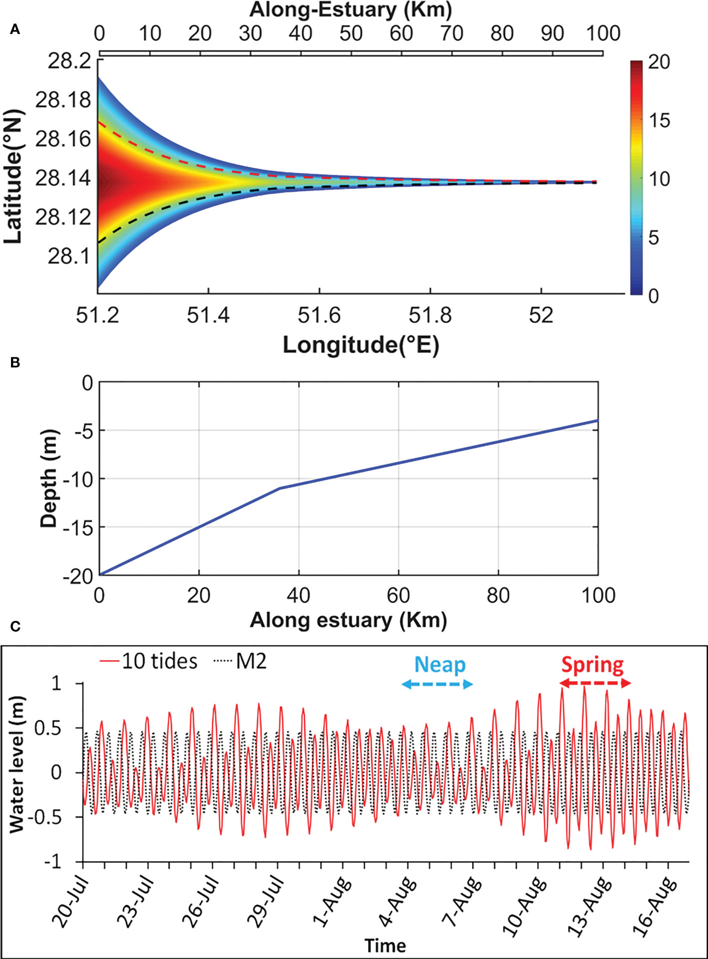
Figure 1 (A) The bathymetry (m) of the idealized basin. The red and black dashed lines show the two symmetrical northern and southern transects between the main axis and the northern and southern coasts, respectively. (B) Along-channel depth variation in the idealized estuary used in numerical simulations. (C) Two 28-day time series of water levels depict the open boundary conditions: only M2 tide in EXP1 and EXP6, and 10 tidal constituents in EXP3 and EXP11. Two 75-hour periods during neap and spring tides in EXP3 are shown by the two blue and red double arrows, respectively, during which average model states are analyzed.

$\begin{array}{ll}W(x)=w_0\text{exp}(-\frac{x}{L_x})& (2)\end{array}$

where $w_0$ and $L_x$ are the width at the mouth (12 km) and the convergence length scale (30 km), respectively. The width of the estuary decreases to ~100 m at the head. The maximum depth at the estuary mouth on the main axis is 20 m (Figures 1A, B). This maximum depth decreases linearly with a rate of 0.25 m/km up to 36 km of the mouth and then with a rate of 0.11 m/km between 36 km and the estuary head (see Figure 1B).

The computational grid is represented by 4180 triangular elements constructed from 150 grid points in the longitudinal direction and 15 grid points laterally (2250 points in total). The resolution of this grid ranges from 2,000 m at the marine open boundary to 10 m at the estuary head. The idealized basin uses 25 sigma layers in the vertical direction.

The location of this idealized funnel-shaped estuary is around 28°N and 51°E, corresponding to the northern coast of the Persian Gulf (Figure 1A). Realistic atmospheric forcing ensures an evaporation rate commensurate with arid coastal conditions (Largier, 2010). This geographic area of the idealistic estuary is selected because it is close to the location of the Mond River Estuary, which behaves as a slat-plug estuary in the warm months (Ghaemi and Gholamipour, 2017).

All numerical simulations are performed for two years (from January 2013 to December 2014), in which atmospheric forcing uses hourly meteorological data from the European Centre for Medium-Range Weather Forecasts (ECMWF, https://cds.climate.copernicus.eu). Wind forcing was disabled to avoid additional complications to the idealistic circulation. Furthermore, temperature and salinity values at the open boundary were taken from the daily reanalysis data of the Persian Gulf provided by the Copernicus Marine Environment Monitoring Service (CMEMS, https://resources.marine.copernicus.eu) during 2013-2014 (730 days).

Eleven different numerical experiments (EXP1-EXP11) served to identify the dynamic differences between various salt-plug estuaries, typical of low latitudes, and to establish canonical patterns of longitudinal and secondary circulations (see Table 1). A low river inflow of 2 m³/s was prescribed at the head of the estuary in all EXP1-EXP11. Additionally, in all experiments, the salinity of the river water was set to zero. The Coriolis force was turned off in EXP1-EXP3 and on in the other eight experiments (EXP4-EXP11). In order to investigate the influence of Coriolis on secondary circulation, the results of EXP1 and EXP2 are compared with the corresponding experiments EXP6 and EXP8 (see Table 1).

TABLE 1

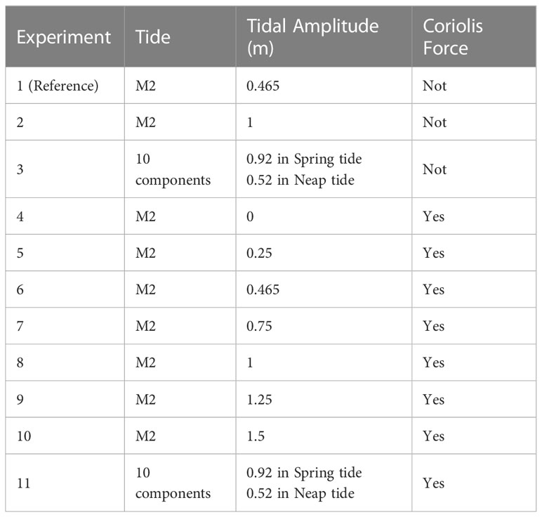
Table 1 Summary of the idealized salt-plug estuarine experiments.

Except for EXP3 and EXP11, tidal forcing was prescribed as the M2 tide only with different amplitudes between 0 m and 1.5 m (see Table 1) to assess the impact of tidal forcing on the salt-plug dynamics. Experiments EXP3 and EXP11 aimed to study the response of the salt plug to spring–neap tidal variability. The tidal forcing in EXP3 and EXP11 used 10 tidal constituents: Q1, O1, P1, S1, K1, N2, M2, S2, K2 and M4 (see Table 2 and Figure 1C). Tide data were taken from the Danish Hydraulic Institute (DHI) global tidal model (Cheng and Andersen, 2010), as Table 2 shows. The amplitude of 0.465 m is selected in EXP1 and EXP6 as it equals M2 amplitude from the 10 tidal components at the approximate experiment location (51.2°E, 28.14°N). Time- (tidally-) averaged model results were obtained from model outputs during 28 days in the summer (20 July - 16 August) of 2014.

TABLE 2

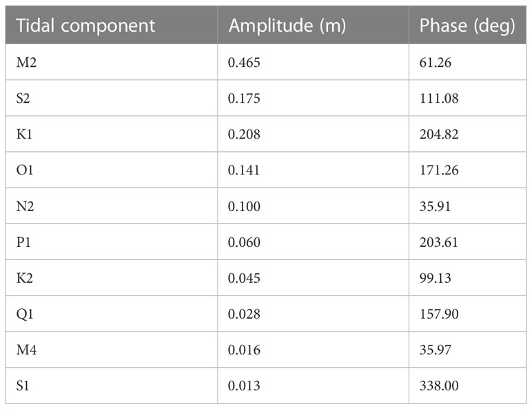
Table 2 The ten tidal constituents extracted from the DHI global model (Cheng and Andersen, 2010) at 51.2°E and 28.14°N used in EXP3 and EXP11.

We used the idealized funnel-shaped basin to consider different tidal forcings in completion with density gradients. The limitations of this study are related to the simplified geometry used. But we are interested in processes, rather than particular systems. Future efforts shall concentrate in examining estuaries with different shapes and geometries.

2.3 Salt flux decomposition in the idealized salt-plug estuary

High evaporation rates (as in the northern coast of the Persian Gulf during the summer), together with the low river inflow (2 m³/s), tend to create a salt plug in the idealistic basin. Thus, there are two areas of relatively lower salinity on both sides of the salt plug. Changing forcings in EXP4-EXP11 should elucidate the competition between density gradient and tidal forcing to change the longitudinal salinity structure in the basin, especially at the salinity-maximum zone.

The instantaneous (time-varying t) total salt flux $F_s(t)$ at each one of the 150 cross-sections along the estuary was calculated as:

$\begin{array}{ll}{F}_s(t)={\displaystyle \sum _{j=1}^{15}{\displaystyle \sum _{k=1}^{25}U(\text{j},\text{k},t)S(j,k,t)A(j,k,t)}}& (3)\end{array}$

where $j$ and $k$ represent the number of cells at cross-sectional and vertical directions, respectively. In fact, the idealized basin includes 150 cross-sections (longitudinal grid points) and 15 lateral grid points ($j$) in 25 sigma layers ($k$). $U$, $S$ and $A$ are the longitudinal velocity, salinity and area of each cell located at the cross-section. Also, the tidally averaged total salt flux $\langle F_s(t)\rangle$ is given by:

$\begin{array}{ll}\langle F_s(t)\rangle =\langle {\displaystyle \sum _{j=1}^{15}{\displaystyle \sum _{k=1}^{25}U(j,k,t)S(j,k,t)A(j,k,t)}}\rangle & (4)\end{array}$

in which the brackets 〈〉 identifies the tidal-averaged value. In order to separate the contribution of different forcings to the salt fluxes, the instantaneous $U(j,k,t)$ and $S(j,k,t)$ can be decomposed into the three components: (1) cross-sectionally and tidally averaged $u_a$ and $s_a$, (2) tidally averaged and cross-sectionally varying $u_e$ and $s_e$, and (3) both cross-sectionally and tidally varying $u_t$, $s_t$, (Lerczak et al., 2006; Aristizábal and Chant, 2015). The three components of velocity define as equations (5), (6), and (7). The salinity decomposition also produces analogous to these equations.

$\begin{array}{ll}{u}_a=\frac{\langle {\displaystyle {\sum }_{j=1}^{15}{\displaystyle {\sum }_{k=1}^{25}U(j,k,t)A(j,k,t)}}\rangle }{\langle {\displaystyle {\sum }_{j=1}^{15}{\displaystyle {\sum }_{k=1}^{25}A(j,k,t)}}\rangle }& (5)\end{array}$

$\begin{array}{ll}{u}_e(j,k)=\frac{\langle U(j,k,t)A(j,k,t)\rangle }{\langle A(j,k,t)\rangle }-u_a& (6)\end{array}$

$\begin{array}{ll}{u}_t(j,k,t)=U(j,k,t)-u_e(j,k)-u_a& (7)\end{array}$

Then, $\langle F_s(t)\rangle$ (equation 4) with neglecting interaction terms yields from the components (equations 5-7) as equation (8) (Lerczak et al., 2006; Aristizábal and Chant, 2015).

$\begin{array}{ll}\begin{array}{r}\hfill \langle F_s(t)=u_a{s}_a{\displaystyle \sum _{j=1}^{15}{\displaystyle \sum _{k=1}^{25}\langle A(j,k,t)\rangle }}+{\displaystyle \sum _{j=1}^{15}{\displaystyle \sum _{k=1}^{25}[u_e(j,k)s_e(j,k)]\langle A(j,k,t)\rangle }}\\ \hfill +{\displaystyle \sum _{j=1}^{15}{\displaystyle \sum _{k=1}^{25}\langle u_t(j,k)s_t(j,k,t)A(j,k,t)\rangle +interactions}}\end{array}& (8)\end{array}$

Generally, the advective salt flux (the first term on the right-hand side of equation 8) is mainly related to river discharge transport, but includes other contributions from meteorological forcing like wind (Valle-Levinson, 2022). Here, the advective term consists of the low-river inflow (2 m³/s) and longitudinal advection from the tidal residual flows (without wind forcing).

The sheared salt transport (the second term on the right-hand side of equation 8) is driven by exchange flows of estuarine circulation (Valle-Levinson, 2022), or by longitudinal density (salinity) gradients (Lerczak et al., 2006).

The third term on the right-hand side of equation (8) indicates the salt transport by tidal pumping that is determined by the covariance between tidal flows and tidal oscillation in salinity. Therefore, this salt flux is related to the phase difference between the longitudinal tidal velocity and salinity. When the salinity and tidal currents are 90° out of phase (are in quadrature), their covariance will be zero (or near zero) and consequently the relevant tidal salt flux tends to zero. In fact, the 90° phase difference is exclusively imposed by longitudinal advection from the tidal flows where the sheared salt transport (induced by gravitational circulation) overcomes tidal pumping salt flux. On the other hand, the salt flux by tidal pumping strengthens when the longitudinal velocity and salinity become out of quadrature under increased processes like tidal mixing and lateral advection. It suggests that the tidal pumping term plays an important role in contributing the net salt flux when salinity extremes occur at time of maximum tidal flood or ebb flows (Aristizábal and Chant, 2015; Valle-Levinson, 2022). In this study, the tidally averaged total salt flux is calculated using Equation (4). Also, Equation (8) is used to compute the contributions from advective, sheared, and tidal pumping salt transports in the tidally averaged total salt flux.

3 Results

3.1 Longitudinal residual circulation in salt-plug estuaries

3.1.1 Basic properties

The time-averaged axial salinity and its longitudinal gradient ($\frac{\partial \text{s}}{\partial \text{x}}$) in the reference scenario (EXP1, see Table 1) demonstrate a typical salt-plug estuary. The salinity in the salt plug, which is in the zone of maximum salinity, is higher than 41.5 between 40 km and 60 km (Figures 2A, D). The zero-value of $\frac{\partial \text{s}}{\partial \text{x}}$, at ~50 km (Figures 2A, B), identifies the position of the salinity maximum. Two estuarine segments (cells) dominate the residual circulation pattern (Figure 2C). In the segment with inverse gravitational circulation, seaward of the plug, surface salinity increases from the mouth to the salinity maximum. Typical gravitational circulation is observed in the upper estuary between the head and the salt plug. In the maximum salinity zone, the mean axial flow nearly cancels out, and vertical stratification is weakest (see Figure 2A). This is consistent with the convergence of surface velocities and the divergence of bottom flow at this area.

FIGURE 2

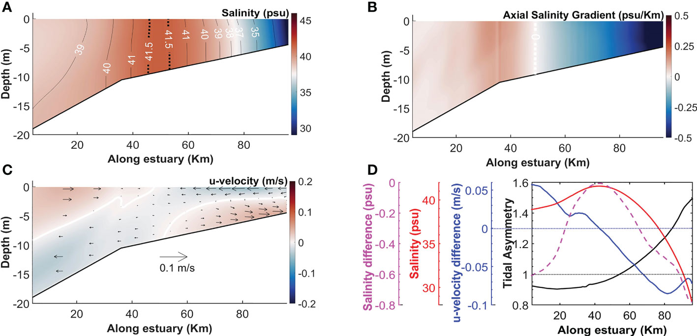
Figure 2 Along-channel profiles of time-averaged salinity (A), axial salinity gradients ($\frac{\partial \text{s}}{\partial \text{x}}$) (B), and axial velocity (C) in EXP1. The depth-averaged tidal current asymmetry along with the time-averaged surface and bottom differences in axial velocity, depth-mean salinity, and surface and bottom differences in salinity are plotted in (D) with different lines. The white dotted line in (B) is zero- $\frac{\partial \text{s}}{\partial \text{x}}$, indicating the border between two estuarine segments. White lines in (C) represent the positions of zero-velocities. The landward direction in the velocity differences is positive in (D).

The surface-to-bottom salinity difference (Figure 2D) provides the positioning of the salt plug. Exactly at the position of the minimum salinity difference, with practically no stratification in EXP1, the surface to bottom axial velocity difference is also zero. The dominance of well-mixed conditions in this area identifies the transition between positive and negative gravitational circulation cells. The change in the sign of the velocity-difference curve (blue line, Figure 2D) represents the changing sense of the circulation cells.

Further insights are drawn by the axial tidal current asymmetry, expressed as the ratio between maximum flood and maximum ebb depth-mean velocities (black line, Figure 2D). A ratio higher than 1 indicates flood-dominated asymmetry. According to this ratio, the direction of tidal current asymmetry changes close to the salt plug so that ebb-dominated asymmetries appear at the inverse gravitational circulation segment while flood-dominated asymmetries develop at the positive gravitational circulation portion.

3.1.2 Fortnightly variations

We extend EXP1 to EXP3 by forcing with ten tidal constituents (spring–neap scenario in Table 1). Results show that the residual circulation after 28 days (Figure 3A) is similar to that from EXP1 (Figure 2C). Two 75-hour intervals during this 28-day period represent neap tide (from 04 August to 07 August 2014) and spring tide (from 11 August to 14 August 2014). Each subperiod covers six M2 cycles (see both periods in Figure 1C). The residual flow for those periods (Figures 3C, E) show that spring-tide patterns resemble the 28-days mean (compare Figures 3A, E). The spring tide residual flow displays seaward displacement of the surface outflow in the positive gravitational circulation that extends throughout the water column (from the surface to the bottom) at the salt plug zone (~50 km) (see Figure 3E). Also, the areas of landward inflow in the spring tide, both surface and bottom, shrink and separate in comparison with those of neap tide (Figure 3C), retreating toward both ends of the estuary (see Figure 3E). In contrast, the inflow areas in neap tides are connected at the salt-plug location (around 50 km in Figure 3C). In general, however, flow patterns in spring and neap tides show essentially the same features. In both cases, the salt plug is in the area that connects (neap) or separates (spring) the residual inflows.

FIGURE 3

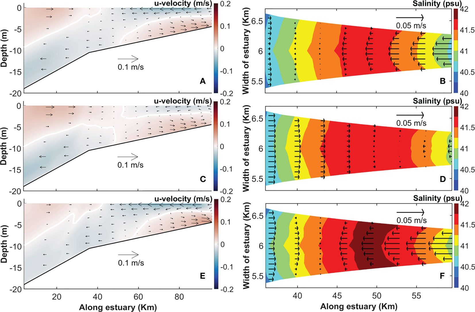
Figure 3 Along-channel profiles of axial velocity in EXP3 (see Table 1). Averaging is for the full neap–spring cycle of 28 days (A), for six M2 periods during neap tide from 04 August to 07 August 2014 (C), and for spring tide from 11 August to 14 August 2014 (E). 2D distribution of surface axial-velocity and salinity corresponding with the periods of (A, C, E) are respectively presented in (B, D, F).

Considering surface longitudinal residual flows across the estuary around the salt plug (36 km – 60 km), shadowed by surface salinity (Figures 3B, D, F), also confirms that the landward surface flows intrude into estuary up to ~km 43 in both averaged 28-day (Figures 3A, B) and spring tide (Figures 3E, F). While the residual landward flows exceeds 50 km in the neap tide (Figures 3C, D). The salt plug is slightly saltier in the spring tide than in the neap tide (see Figures 3D, F), owing to higher tidal mixing during spring tides (Geyer and MacCready, 2014) that is associated with higher landward salt transport by tidal advection in the spring tide. Also, tidal pumping of salt shows a landward direction in the spring tide contrary to the neap tide (see section 4.2).

From the different residual flow fields at the salinity maximum zone (around 50 km) in the spring-neap transition, it is reasonable to expect that dissimilar lateral shears in the axial velocities $\frac{\partial u}{\partial y}$ and the axial change in salinity should lead to differential advection $\frac{\partial u}{\partial y}\frac{\partial s}{\partial x}$ (equation 1), resulting in generation of different lateral flows. Thus, fortnightly variations in lateral flows should be evident around the salt-plug region, as described in the following section.

3.2 Lateral circulation in salt-plug estuaries

3.2.1 The impact of earth’s rotation

Time-averaged lateral shears of along-channel velocities ($\frac{\partial \text{u}}{\partial \text{y}}$) in the inverse estuarine segment (at 25 km) have opposite signs at the surface to those in the positive estuarine segment (at 75 km) (Figures 4A, E). Also opposite is the sign of the along-channel salinity gradients ($\frac{\partial \text{s}}{\partial \text{x}}$) on both sides of the salt plug (see Figure 2B). Therefore, their product ($\frac{\partial \text{s}}{\partial \text{x}}\frac{\partial \text{u}}{\partial \text{y}}$), representing differential advection, has the same sign in the two estuarine segments. Differential advection thus builds converging flows at the surface in the deep channel (Figures 4B, F). Lateral circulation cells are rather symmetric because the model setup is symmetric (no Coriolis force or asymmetric bathymetry in EXP1). Although the cells show similar overall structure at the two cross-sections, they have marked differences along the channel in terms of the proportions occupied by positive or negative flows.

FIGURE 4

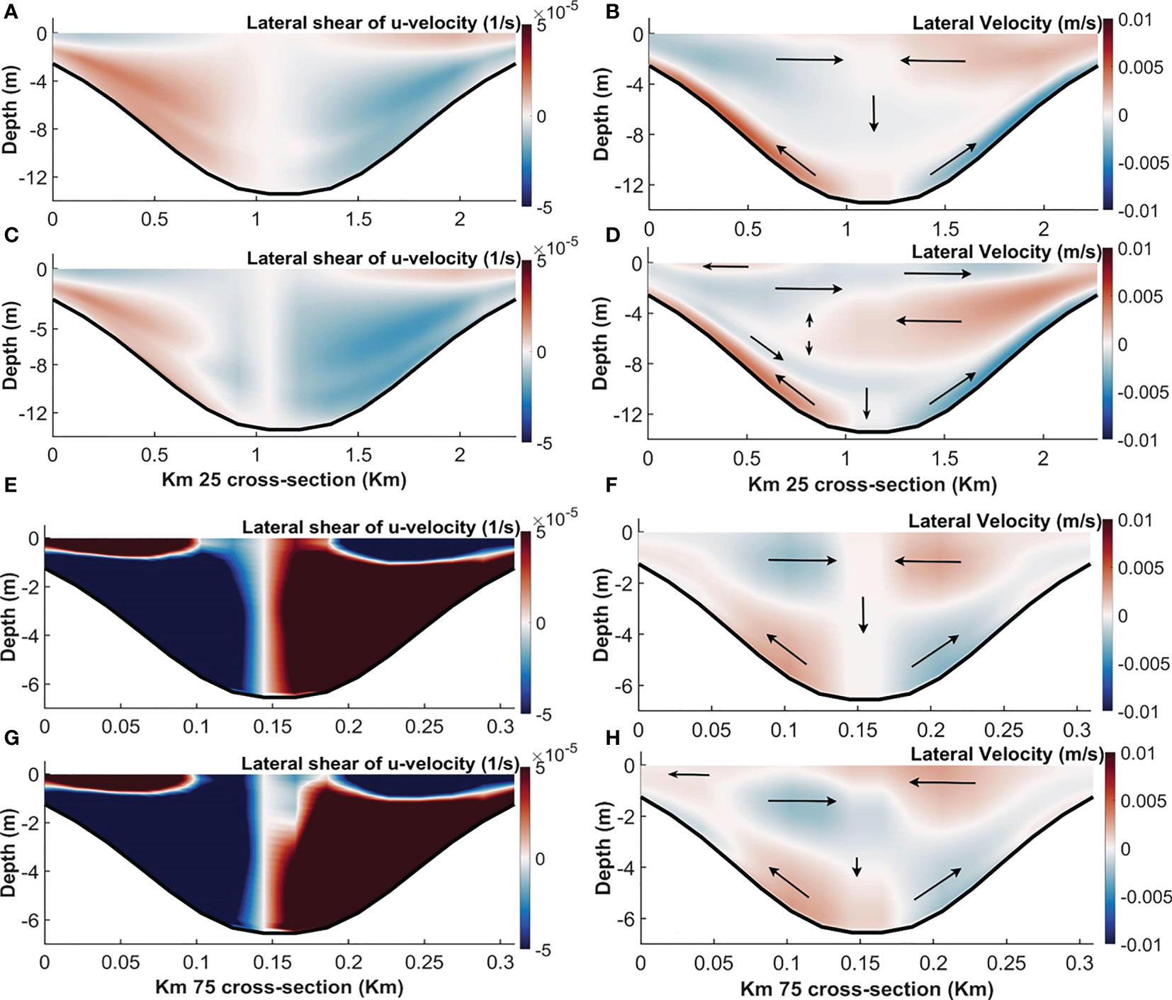
Figure 4 Time-averaged lateral shear of along-channel velocities ($\frac{\partial \text{u}}{\partial \text{y}}$) (A, C, E, G) and lateral velocities (B, D, F, H) along the cross section at 25 km (A–D) and 75 km (E–H) from the mouth in EXP1 (A, B, E, F) and EXP6 (C, D, G, H). Red and blue colors in lateral velocities represent leftward and rightward velocities, respectively, looking into the estuary.

The impact of Earth’s rotation on the salinity field is straightforward as the maximum salinity zone is displaced to the right, looking seaward. More revealing is that the values of $\frac{\partial \text{u}}{\partial \text{y}}$ in EXP6 at 25 km display asymmetries (compare Figures 4A, C). At the narrow part of the channel (75 km), the asymmetries in $\frac{\partial \text{u}}{\partial \text{y}}$ are less evident (compare Figures 4E, G). However, the structure of the lateral velocities are changed along both sections, especially in the upper layers (compare Figures 4B, D, as well as Figures 4F, H) after activating Coriolis accelerations. The section close to the mouth is distinguished by a near-surface diverging cell (Figure 4D).

Near the bottom, on the other hand, lateral flows change little from EXP1 (without Coriolis accelerations, Figures 4B, F) to EXP6 (with Coriolis force, Figures 4D, H) in both cross-sections. In fact, experiments with and without Coriolis (EXP1 and EXP6) reveal that Coriolis deflection alters lateral circulation even in narrow cross-sections near the head of the estuary, reproducing cross-sectional flow asymmetries such as those reported by (Valle-Levinson et al., 2003) and (Chant, 2010). The bottom line is that asymmetries tend to be enhanced at the surface and reduced near the bottom (see Figure 4). This is consistent with the results of (Johnson and Ohlsen, 1994). Using laboratory experiments over a simulated ocean channel (“trough”), they demonstrated that the surface secondary (Ekman) flows vary along the channel, while the flows in the bottom Ekman layer almost have the same structure along the channel. Moreover, (Friedrichs and Valle-Levinson, 1998) showed that secondary circulations driven by Coriolis forcing are stronger at the surface and weaker near the channel bed, considering positive estuaries at the dominant tidal frequency. Both secondary and longitudinal tidal currents were surface intensified, which suggests that Coriolis accelerations cannot be entirely balanced by a barotropic pressure gradient.

Thus, in the absence of Coriolis acceleration, the dominant dynamic mechanism driving lateral flows is differential advection. However, Coriolis influences lateral circulations, as diagnosed with the Ekman and Kelvin numbers (Garvine, 1995), (Table 3).

TABLE 3

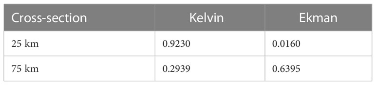
Table 3 The time-averaged values of nondimensional vertical Ekman and Kelvin numbers in the cross-sections at 25 km and 75 km in EXP6.

Table 3 presents these number values for the two cross-sections of 25 km and 75 km from EXP6. Since both the width and depth decrease from the estuary mouth to the head, the Coriolis impact (Kelvin number) increases quite substantially with decreasing distance to the mouth (compare the two Kelvin numbers in Table 3). In contrast, the Ekman number (frictional effects) increases with decreasing distance to the head (see the Ekman number values in Table 3).

3.2.2 Influence by differential advection

3.2.2.1 Along-channel evolution

The cross-channel sections in Figure 4 are different enough to question any conclusions on secondary flows drawn from only two sections. Therefore, lateral velocities along the northern along-estuary line (from Figure 1A) provide a relatively more comprehensive picture (Figure 5A). This line’s position, away from the thalweg, should illustrate robust lateral velocities. Because of the symmetric flow structures in EXP1, the southern along-estuary line mirrors the northern line (not shown).

FIGURE 5

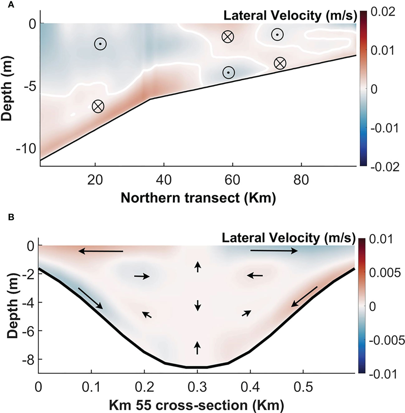
Figure 5 Time-averaged lateral velocities (A) along the northern transects shown in Figure 1, and (B) along the cross section at 55 km from the mouth in EXP1. Red and blue colors in (A) represent northward and southward velocities, respectively. Leftward and rightward velocities looking into the estuary are identified in (B) by red and blue colors, respectively.

Over most of the estuary, the lateral circulation in EXP1 is typically structured in two symmetric cells, one north (see Figure 5A) and one south of the thalweg. The northern cell is formed in the inverse estuarine segment, between the mouth and the salt plug. In this cell, lateral near-surface velocities converge toward the thalweg and diverge at the bottom. In the positive estuarine segment, the residual lateral flow is more complex. Close to the head of the estuary (>70 km in Figure 5A), there are two cells one above the other. At the salt-plug zone, between 50 km and 70 km, the directions of lateral velocities reverse. Actually, the pattern illustrates a divergent surface cell at 55 km (also shown in Figure 5B). This is in opposition to the convergence of axial velocities in the same area (Figure 2C), that is the surface axial inflow and outflow approaching each other (the surface longitudinal convergence occurs) at the salt plug zone (see km 50 in Figure 2C). Conversely, the bottom longitudinal flows diverge from each other in this zone.

3.2.2.2 Spring-neap lateral flows and salinities at the salt plug

The time-average lateral flows at 50 km in neap and spring tide show similar structure across the basin, but with opposite signs (Figures 6A, E; see the neap and spring averaging periods in Figure 1C). During the neap period, the lateral flow shows circulation cells conducive to upwelling in the deep channel (Figure 6A). Conversely, spring tides lateral flows illustrate downwelling in the deep channel (Figure 6E). As a result, the time-averaged salinities are also redistributed by the relevant lateral circulations across the section in the neap and spring tides (Figures 6B, F). The upwelling flows in the center channel lift isohalines in the neap tide (Figure 6B), whereas lying down lateral flows depress isopycnals in the center channel, creating a saddle shape in the isohalines associated with the upwelling flows in both sides of shallow shoals during the spring tide (Figure 6F).

FIGURE 6

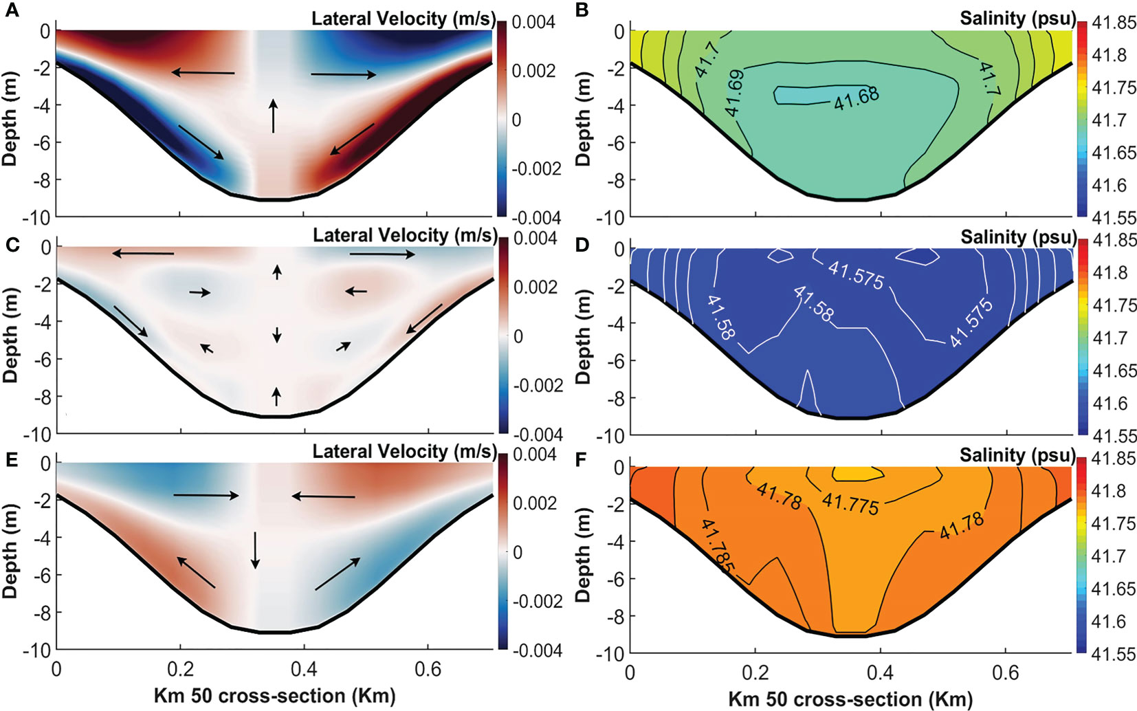
Figure 6 The time-averaged lateral velocities (A, C, E) and salinities (B, D, F) along the cross section at 50 km during neap tide (A, B), full neap–spring cycle (C, D) and spring tide (E, F) from EXP3. Red and blue colors in velocities identify leftward and rightward velocities, respectively, looking into the estuary.

A basic difference between spring-neap secondary circulations is that lateral circulation is stronger during neap than spring tide because of weaker mixing (Geyer and MacCready, 2014), (also see isohalines at the thalweg in Figures 6B, F). Actually, under weak stratification, such as in the salt-plug zone (see Figures 2D, 6B, F), the dynamics are consistent with the results of (Geyer, 1993). However, as stratification increases, the second term of the right-hand side of equation (1), ($\frac{\partial w}{\partial y}\frac{\partial s}{\partial z}$), tilts the halocline with the secondary flows. This advective term produces a baroclinic pressure gradient that opposes the lateral shear mechanism and consequently tends to shut down the secondary flows, consistent with Chant, 2010.

This result agrees with the study by (Lerczak and Geyer, 2004), which claims that the structure of the secondary circulations could change in the transition from neap to spring tides. At the salt-plug zone, it actually reverses.

On the other hand, the secondary circulations during the full neap–spring period (Figure 6C) show more similarity with the neap than with the spring period. The secondary circulations redistribute isohalines in the vertical shape with upwelling them near the surface in the center channel during the full neap–spring period (Figure 6D).

3.3 Responses to increasing tidal amplitude

This section presents the relative influence of tidal forcing vs density gradients on the salt-plug position in the estuary. Eight experiments (EXP4 to EXP11) that portray, through the temporally and depth-averaged axial salinity, that the salt plug is not only enhanced with tidal forcing but it is also transported landward at tidal amplitudes higher than 1 m (the meso-tidal estuaries of EXP8-EXP10, Figure 7A and Table 4). While the salt plug moves landward from zero-tide (EXP4) to EXP5, it then moves seaward in microtidal experiments EXP5, EXP6 (~0.5 m tide), EXP11 (the spring-neap experiment) and EXP7 (with tidal amplitude of 0.75 m) (see Table 4), with a change in salinity of only around 1 psu at the salt plug (see Figure 7A). These responses are attributed to the competition between tides and density gradients dominating the momentum balance, and the prevalence of tidal pumping or sheared transport in driving the salt balance.

FIGURE 7

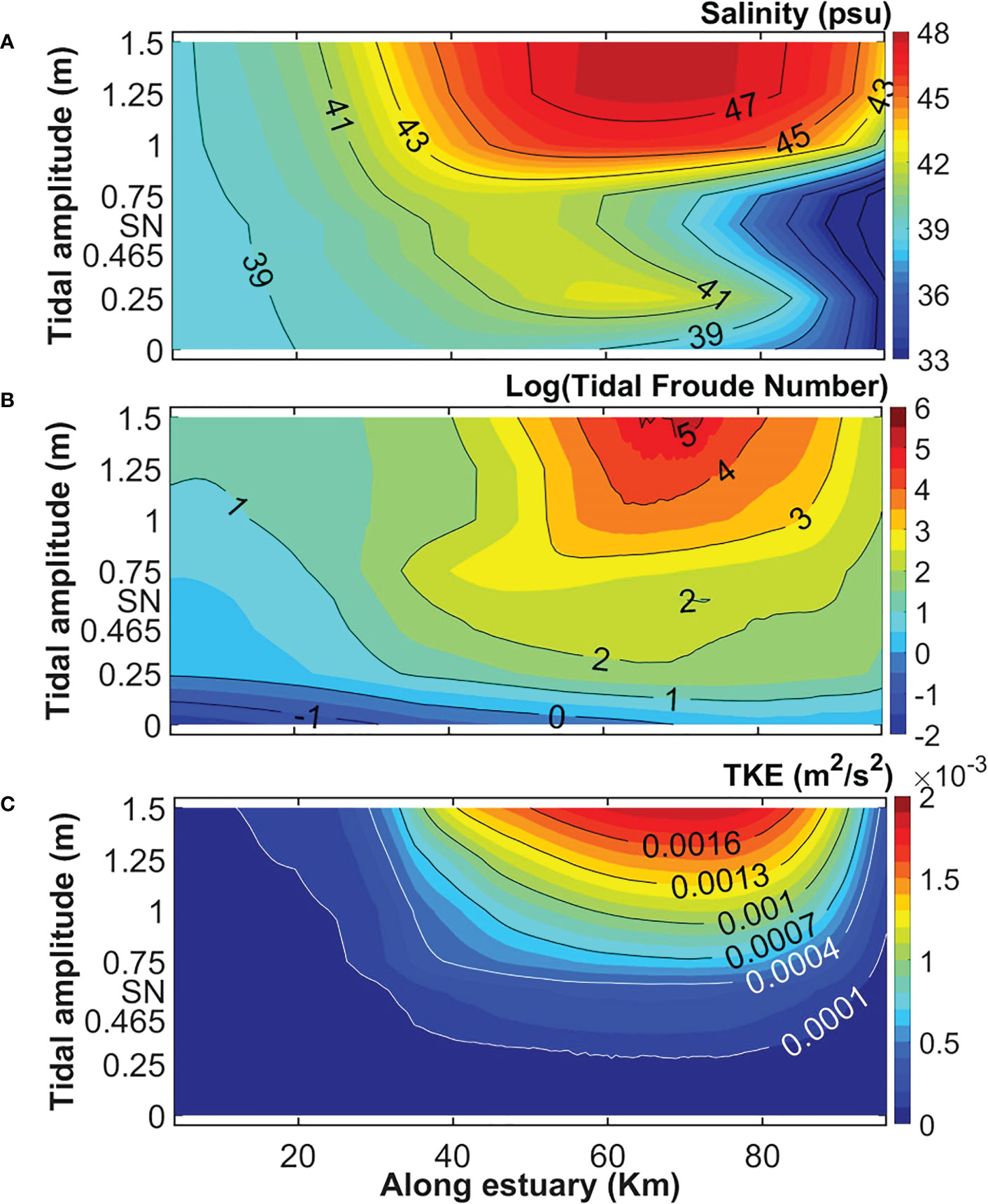
Figure 7 The tidally averaged depth-mean axial salinity (A), the logarithm of tidal Froude number (B) and the turbulent kinetic energy TKE (C) from 8 scenarios of EXP4-EXP11 (see Table 1), as a function of distance from the estuary mouth (x-axis) and tidal amplitudes at the estuary mouth (y-axis). “SN” on the y-axis stands for the spring-neap scenario of EXP11.

TABLE 4

Table 4 The distances of the salt plug centers (where $\frac{\partial s}{\partial x}=0$) from the estuary mouth in the 8 numerical experiments of EXP4-EXP11 (These distances are considered as $L_{\rho }$ to compute the tidal Froude number).

For the momentum balance competition, the densimetric tidal Froude number ($F{r}_T$) (Figure 7B) is used according to the study of (Valle-Levinson, 2021) as $F{r}_T=\frac{L_{\rho }}{L_T}\frac{U_T^2}{\acute{g}D}$ in which $U_T$ is the along-basin tidal current amplitude. $\acute{g}=g\frac{\Delta \rho }{{\rho }_{up}}$ is the reduced gravity determined by the density difference ($\Delta \rho$) between the upper (${\rho }_{up}$) and lower (${\rho }_{low}$) layers. $\text{D}$ is the mean water depth. $L_{\rho }$ and $L_T$ denote horizontal length scales associated with density and tidal forcing, e.g., the salt intrusion length and the tidal excursion, respectively. $L_T=\frac{T{U}_T}{\pi }$ in which $T$ is the tidal period (Valle-Levinson, 2022) and equals the M2 period (12-hour-and-25-minute) in this study as M2 is the unique tidal forcing in EXP4-EXP10 (see Table 1) and acts as the strongest tidal component in EXP11 with the mixed mainly semidiurnal tidal regime (see Table 2 and Figure 1C). Also $L_{\rho }$ is considered as the distance from the estuary mouth in which the direction of $\frac{\partial s}{\partial x}$ changes from the inverse segment to the positive segment in the relevant salt-plug estuary according to Table 4. Figure 7B demonstrates that the logarithm of tidal Froude number higher than 3 (tidal forcing 3 orders of magnitude ≥ density gradients) occurs only for tidal amplitudes higher than 1 m (EXP8-EXP10) from ~ km 50 to ~ km 90 where salt plugs have salinity higher than 45 psu.

Thus, Figures 7A, B introduce the threshold of “log(tidal Froude number)=3” as the condition under which the tidal forcing can overcome the density gradient, and consequently salinity inside the salt plug zone and its location is dominated by tides. This is a new finding because salt plug estuaries have been exclusively attributed to density-driven flows.

The variations in quantity of salinity inside, and the location of the salt plug can be explained by different tidal forcing potentials of the microtidal and mesotidal estuaries, which impose different salt transports along the estuary. The analysis of different salt flux terms is discussed in Section 4.2.

The tidally averaged depth-mean axial turbulent kinetic energies (TKE) from EXP4 to EXP11 (Figure 7C) are consistent with the tidal Froude number distributions. Also, comparing this figure with Figure 7A indicates that the TKE, a measure of vertical mixing, increases from the inverse and positive estuarine segments toward the salt plug, especially at the meso-tidal estuaries.

In order to depict the influence of increasing tidal forcing on the longitudinal and lateral flows, these results from the meso-tidal EXP2 (with 1 m M2-tide at the mouth) in Figure 8 are compared with those in the micro-tidal EXP1 (with 0.465 m M2-tide at the mouth) in Figure 2.

FIGURE 8

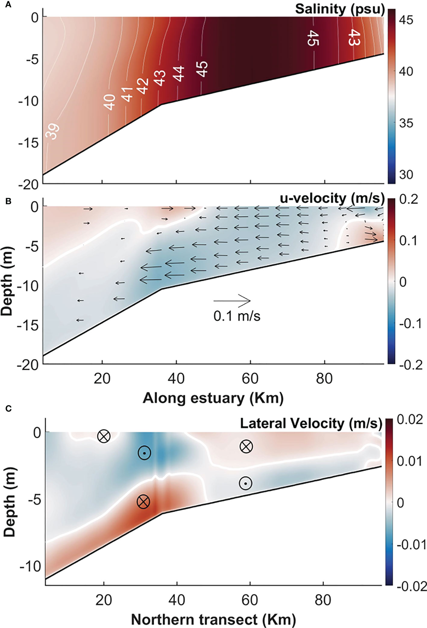
Figure 8 Along-channel profiles of time-averaged (A) salinity and (B) axial velocity along the main axis and (C) lateral velocities along the northern transect in EXP2.

When the tidal energy increases in EXP2 compared with that in EXP1, the freshwater rarely reaches the mid-estuary and is trapped near the estuarine head. It means that the positive estuarine segment weakens from the micro-tidal EXP1 to the meso-tidal EXP2 (compare Figures 2A with 8A, and 2C with 8B). The trend associated with more landward salt transport mainly by tidal advection (see Section 4.2), creates a stronger and more extensive salt plug in EXP2. In the other words, the salt plug in the meso-tidal EXP2 shows a much longer extension along the estuary, between 30 km and 90 km, and the salinity there is higher, from 42-45 psu (compare Figure 2A and Figure 8A). The zone of seaward longitudinal flows increases in size in EXP2 (compare Figure 2C and Figure 8B). The decrease in the area of landward flow is very strong at the bottom of the positive estuarine segment in Figure 8B in comparison to that in Figure 2C.

The landward expansion of the salinity-maximum zone and the contraction of the positive estuarine segment from EXP1 to EXP2 corresponds with a similar expansion and contraction in the lateral flows of EXP2 (compare Figures 5A and 8C). Figure 8C actually reveals a simple structure of lateral velocity in the mesotidal EXP2, particularly in the area of the positive estuarine segment. There, the situation is opposite to that in the salt plug: surface flows tend to diverge from the channel axis (thalweg) and converge at the bottom (Figure 8C). The increase in tidal amplitude in EXP2 also resulted in the formation of two surface circulation cells (on both sides of the thalweg) close to the mouth with an opposite sense of rotation to that of the dominant (converging toward the thalweg) cells.

4 Discussion

4.1 Longitudinal and lateral divergences

The ratio between tidally averaged lateral divergence (dv/dy) to longitudinal divergence (du/dx) is calculated at surface and bottom layers (Figures 9A, B) to determine their relative contribution to the divergence patterns associated with the salt plugs. In all eight scenarios (EXP4-EXP11), dv/dy is stronger than du/dx at the surface and bottom layers (Figures 9A, B). Thus, lateral divergence dominates the overall divergence, especially for the micro-tidal experiments.

FIGURE 9

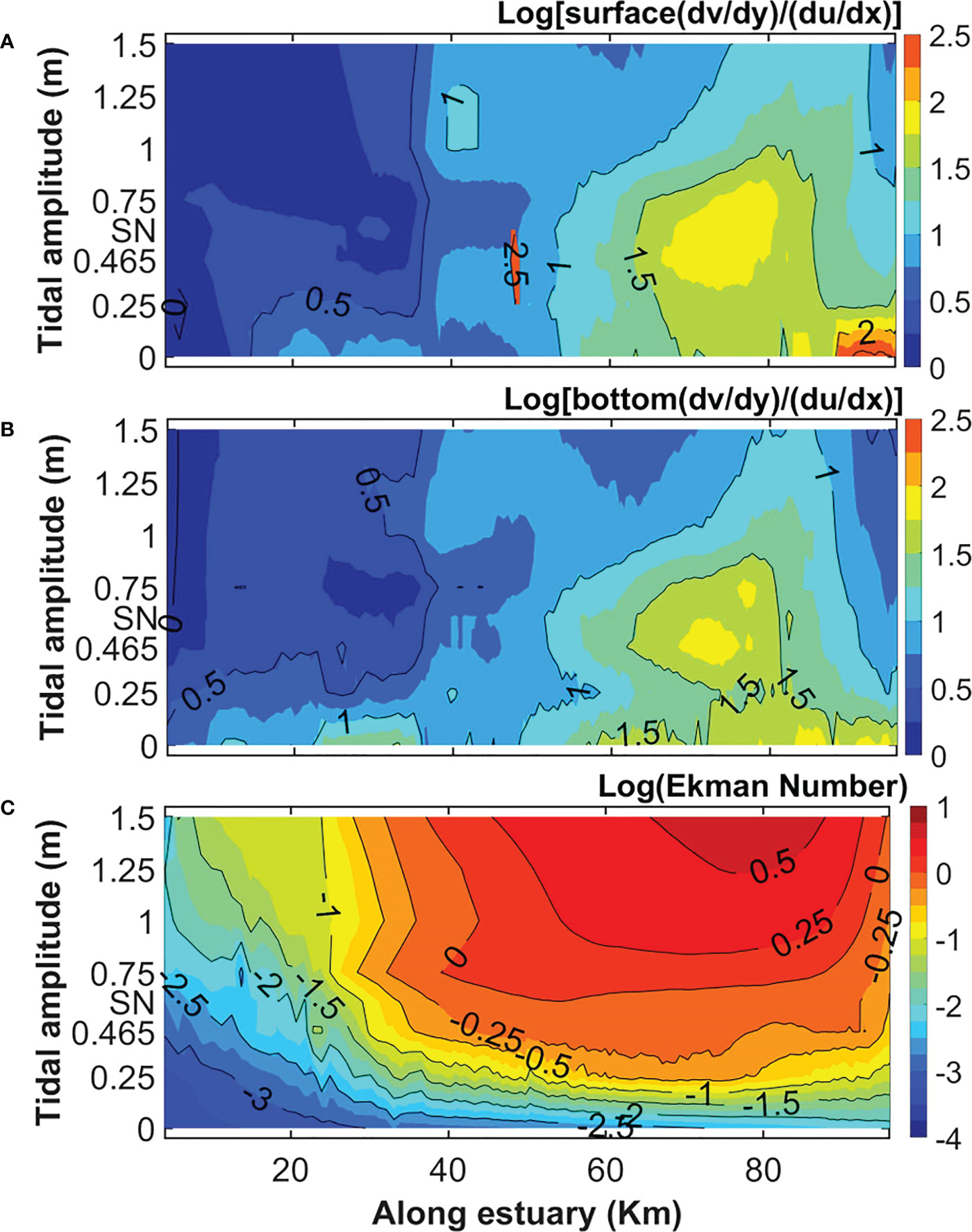
Figure 9 The logarithm of the ratio tidally averaged dv/dy to du/dx for surface (A) and bottom (B) layers as well as the logarithm of Ekman number (C) from 8 scenarios of EXP4-EXP11 (see Table 1), as a function of distance from the estuary mouth (x-axis) and tidal amplitudes at the estuary mouth (y-axis). “SN” on the y-axis stands for the spring-neap scenario of EXP11.

Also, the greatest ratios of dv/dy to du/dx are observed at the surface layer inside the salt plug of EXP11 (around 50 km, Figure 9A), resulting from a high value of dv/dy (see Figure 6C) and a low ratio of du/dx (see Figure 3A) at the same area. It suggests the importance of lateral divergent (longitudinal convergent) surface flows in the full spring-neap tidal cycle (28 days). Thus, lateral flows have a more important role than longitudinal flows in causing divergences. Section 3.2 (see Figure 4 and Table 3), it makes evident that Coriolis forcing affect the lateral circulations driven by the differential advection at the two cross-sections.

This is confirmed by estimates of Ekman number that is expressed as $E=\frac{A_z}{f{D}_{\max }^2}$ in Figure 9C where $A_z$ and $f$ are the vertical eddy viscosity and the Coriolis parameter respectively. $D_{max}$ is the maximum water depth (the thalweg depth) of each cross-section. Coriolis forcing becomes higher than frictional effects (negative log of Ekman number) near the mouth for all the experiments and near the head of the micro-tidal experiments (Figure 9C). Positive log of Ekman numbers (stronger frictional effects than Coriolis forcing) nearly coincide with salt plugs attaining salinity > 45 psu and with logarithm of tidal Froude number > 3 (Figures 9C, 7A, B). Approaching the tidal Froude number (Figure 7B), TKE (Figure 7C) and Ekman number (Figure 9C) to their peak values inside the salt plug (Figure 7A) signifies that the nonlinearities reach their maximum values at the salt plug, particularly in the meso-tidal estuaries.

4.2 Link between salt-plug zones and salt-flux components

The phase difference between tidal velocity and salinity in the inverse (20 km) and positive (80 km) estuarine subsystems of EXP11 with a complex tidal regime tends to -90° and +90°, respectively (Figures 10A, C). It means that salinity reaches its maximum close to high water in the positive estuarine segment. Analogously, minimum salinities appear at low water in the positive segment (see the red and blue plots in Figure 10C). The opposite occurs for the inverse segment of the estuary (the red and blue plots in Figure 10A). The transition of the tidal flow-salinity phase difference from -90° to +90° should appear at the salt-plug zone, which explains the appearance of harmonics with ~6-hour periodicity at the plug (see Figure 10B). Inside the salt-plug zone (~ 48 km), salinity reaches maxima during peak ebb and peak flood, and its minima during high-water slacks and low-water slacks. The tidal axial flows and tidal level have also a phase difference of 90° throughout the shallow salt-plug estuary (see the black and blue plots in Figures 10A, B, C), signifying the formation of the standing wave in the estuary. In short and/or shallow estuarine embayments with negligible reflection, the phases of tidal velocity and water level are in quadrature, which specify classic standing waves (Friedrichs, 2010; Hosseini et al., 2016). Due to the landward convergence of the idealized geometry (effects of the convergent channel overcome friction effects), (see Figures 1A, B), both amplitudes of tidal flow and water-level increase in the landward direction (see the black and blue plots in Figure 10A–C). The amplitudes grow from ~0.3 m/s and ~0.93 m at 20 km (Figure 10A) toward the salt plug (~0.7 m/s and ~1.1 m in Figure 10B) and to the head (such as ~0.8 m/s and ~1.4 m at 80 km in Figure 10C). Also, the peak flood is stronger than the peak ebb at 80 km (the black plot in Figure 10C) indicating the tidal flood-dominated asymmetry at the upper estuary. The opposite asymmetry of ebb-dominance (stronger the peak ebb velocity than that during flood tide) is observed at the lower estuary of 20 km (see the black plot in Figure 10A) as Figure 2D shows these two contrary asymmetries.

FIGURE 10

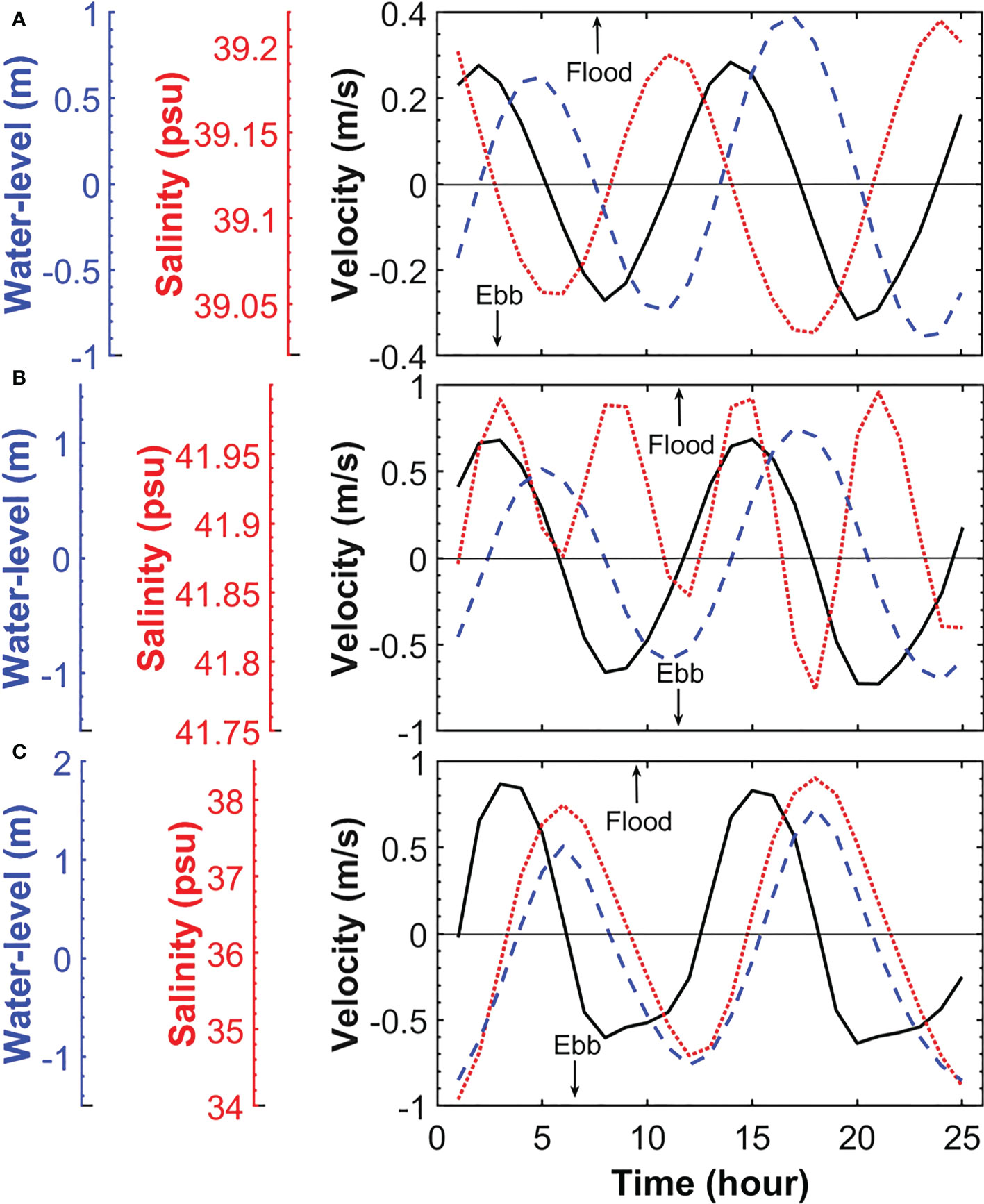
Figure 10 Tidal variations in depth-mean axial velocity (the thick black line), salinity (the dotted red line) and water-level (the dashed blue line) on the main channel axis at ~20 km (A), ~ 48 km (B) and ~ 80 km (C) in EXP11 during 25 hours.

The lower periodicity (higher frequency ~2 times) of the salinity fluctuation than the corresponding tidal current (Figure 10B) is associated with high tidal mixing inside the salt plug (see Figures 2D and 7C). In fact, the occurrence of extreme tidal fluctuations of salinity coincident with maximum tidal flood and ebb flows at the salinity maximum zone (Figure 10B) might be influenced by high tidal mixing there (Figure 7C), suggesting a considerable change of tidal pumping of salt in the salt plug.

The salt-flux decomposition along the estuary illustrates the advective salt flux (in the absence of wind forcing) as the dominant mechanism in both micro-tidal EXP5 (Figure 11A) and meso-tidal EXP10 (Figure 11C). In fact, the advective process (dominantly driven by tides) induces a landward salt flux that exponentially decreases along the estuary in the landward direction. This salt flux overcomes the other salt flux mechanisms, thus driving a landward total salt flux at the estuary and consequently reinforcing salinity maximum zone. The tidal advective salt flux is stronger in the mesotidal EXP10 than in the microtidal EXP5 particularly at the middle of estuary. For instance, the advection drives ~2200 m3/s psu in EXP10 that drops to ~250 m3/s psu in EXP5 at 40 km (see Figures 11A, C), which induces much stronger salt plug in EXP10 than in EXP5 (see Figure 7A). The advective salt flux is slightly weakened by the seaward sheared salt flux near the estuary mouth, especially in the microtidal estuary EXP5. The sheared salt flux remains seaward at the inverse estuarine segment (0 km – ~50 km) in both micro-tidal EXP5 and meso-tidal EXP10 (see Figure 11A, C). A sudden change observes at the advective flux and consequently at the total salt flux, especially in EXP10, around 36 km, where the bottom steepness change suddenly (see Figure 1B). Also, the tidal pumping of salt is close to zero in EXP5 but it experiences a low peak around the point of 36 km in EXP 10 (see Figures 11A, C). It can result from interactions between tidal flows and bathymetry changes.

FIGURE 11

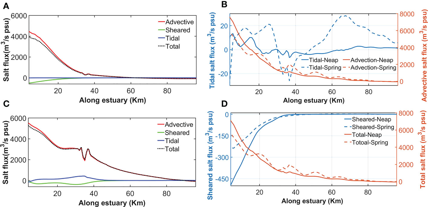
Figure 11 The distribution of the time averaged different salt flux terms along the estuary from the micro-tidal EXP5 (A) and from the meso-tidal EXP10 (C), (see Table 1). Comparing the time averaged (75 hours) neap-spring salt fluxes from the tidal and advective terms (B) and from the sheared and total salt fluxes (D) in EXP3. The total salt flux equals advective plus sheared and tidal pumping. Positive fluxes are landward.

In addition, higher tidal mixing during spring tide than in the neap tide particularly at the salt plug (around 50 km) of EXP3 (see Figures 6B, F) coincides with landward and seaward salt transport by tidal pumping at the salt plug in the spring and neap tides, respectively (see around 50 km in Figure 11B). Also, stronger landward advective salt flux occurs around 50 km in the spring tide than in the neap tide. Both changes in tidal pumping and advective salt transports in the spring-neap transition impose stronger salinity maximum zone during the spring tide (see Figures 3D, F).

In the neap tide, the tidal pumping of salt is relatively weak and shows a seaward transport at ~20 km – ~65 km, while it becomes stronger in the spring tide and indicates seaward directions close to the mouth and around 36 km (with the sudden change in the bottom steepness) during the spring tide (Figure 11B). The latter indicates a robust interaction between strong spring-tidal flows and bathymetry changes (see Figure 11B).

In both spring and neap tides, the time-averaged total salt flux is dominated by the advective flux (see Figures 11B, D). The seaward (negative) sheared salt flux is stronger in the neap tide than in the spring tide near the mouth because of higher longitudinal salinity (density) gradients driving stronger stratification during neap tide (Geyer and MacCready, 2014). This salt flux shows insignificant changes at the upper estuary (~40 km – 100 km), particularly inside the salt plug (around 50 km) in the spring-neap tidal cycle (see Figure 11D).

The advective, tidal pumping, sheared, and total salt fluxes depend on tidal forcing (experiments of EXP4-EXP11, Figure 12). The advective process mainly induces landward salt flux (with positive values) in the lower inverse estuary and at the salinity maximum zone. Seaward advective salt transport (with negative values) in the upper positive estuarine segment is driven by the low river discharge of 2 m³/s (see Figure 12A). The seaward advective salt flux extends longer at the microtidal estuaries (EXP4-EXP7 and EXP11 with tidal amplitudes<1) than in the mesotidal experiments (EXP8-EXP10) upon decreasing tidal amplitude in the microtidal estuaries. The tidal pumping of salt almost shows seaward (negative) values at the salinity maximum zone of all the experiments (Figure 12B). In EXP4 and EXP5, the negative values of this salt flux also occur in the lower inverse estuary while a peak landward tidal salt flux around 36 km at the mesotidal estuaries indicates the importance of interactions between strong tidal flows and bathymetric changes (see Figure 12B). The sheared salt flux is usually landward in positive estuaries (Lerczak et al., 2006; Aristizábal and Chant, 2015; Valle-Levinson, 2022), which agrees with positive (landward) values of this salt flux in the upper positive estuarine segment of the microtidal salt-plug estuaries (Figure 12D). Conversely, the sheared salt flux becomes seaward at the lower inverse estuarine segment of all the salt-plug estuaries. The sheared flux shows an unusually weak seaward values close to the head of mesotidal salt-plug estuaries (see Figure 12D), which may result from overcoming tidal forcing over density gradients, as the sheared salt flux is driven by density gradients.

FIGURE 12

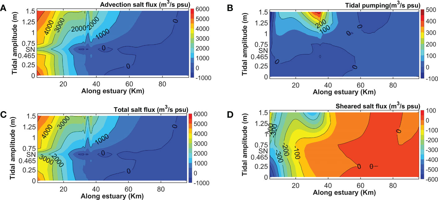
Figure 12 The time averaged advective (A), tidal pumping (B), total (C) and sheared (D) salt fluxes along the estuary from 8 scenarios of EXP4-EXP11 (see Table 1), as a function of distance from the estuary mouth (x-axis) and tidal amplitudes at the estuary mouth (y-axis). “SN” on the y-axis stands for the spring-neap scenario of EXP11 and positive fluxes are landward.

The salt transport by tidal advection (Figure 12A) dominates the fluxes by the tidal pumping (Figure 12B) and sheared (Figure 12D) terms throughout the estuary, which drives a similar total salt flux (Figure 12C). Therefore, in the lower estuary, landward total salt flux persists in all experiments (see Figure 12D). Thus, the salt plug formation and its location are controlled by high evaporation rates compared with low-river inflows associated with the total (net) salt transport consisting of three main salt fluxes induced by advection, tidal pumping and gravitational circulations (sheared term). The two latter terms (gravitational circulations and tidal pumping) cannot overcome the advective salt flux (in the absence of wind forcing). The secondary circulations can mainly redistribute isohalines laterally (see Figures 6B, D, F).

4.3 A framework for salt-plug estuaries based on Ekman and tidal Froude numbers

The logarithm of Ekman number ($E$) along the main axis approaches the highest value in the salt-plug zone (see Figures 7A and 9C) because of high values of vertical eddy viscosity $A_z$, where the longitudinal surface flows converge and the longitudinal bottom flows diverge (for example see Figures 2C and 8B). This maximum Ekman number rarely exceeds 1 (($Log(E)$ = 0) in the micro-tidal EXP4-EXP7 and EXP11 (Figure 9C) but it becomes higher than 1.8 ($Log(E)>0.25$) in the meso-tidal EXP8-EXP10 (see Figure 9C). The sheared bottom exchange flows in the region with high values of the Ekman number (within the salinity-maximum zone) resemble the laterally sheared flow mechanism suggested by Valle-Levinson (2008) in positive estuaries. Using laterally varying (channel-shoals) idealistic bathymetry, Valle-Levinson (2008) suggested that strong frictional control ($E>1$) leads to horizontally sheared exchange flows in positive estuaries, independent of the width of the basin. Apparently, high frictional effects result in laterally sheared longitudinal flow patterns in both studies even though the salt-plug estuarine properties in this study are different from those in positive estuaries (the idealized positive estuary with high frictional effects and the narrow positive estuary of the Hudson River with moderate to strong friction) of Valle-Levinson (2008)‘s study.

In addition to the high values of the Ekman number in the salt-plug zone, maximum values of tidal Froude number ($F{r}_T$) also occur there (see Figures 7A, B). The logarithm of $F{r}_T$ rarely reaches 3 ($F{r}_T=1000)$ in the microtidal salt-plug estuaries (EXP4-EXP7 and EXP11) while this logarithm passes 3 ($F{r}_T>1000)$ in the meso-tidal EXP8-EXP10 (Figure 7B). Valle-Levinson (2021) suggested a general framework based on tidal Froude ($F{r}_T$) and Ekman ($E$) numbers. This framework did not consider salt-plug estuaries so it is discussed here for different micro-tidal and meso-tidal funnel-shaped estuaries of EXP4-EXP11.

Based on this classification and considering the competition between Coriolis acceleration and friction, the entire estuarine basin of the salt-plug estuaries with tidal amplitudes lower than 0.25 m (at the mouth) belongs to the “deep (rotational)” space (see Figure 9C) in which $E\le 0.1$ ($Log(E)\le -1$). In the funnel-shaped salt-plug estuaries with tidal amplitudes higher than 0.25 m, the section between 0 km and ~25 km along the axis of the estuary is also classified as the “deep (rotational)” space (see Figures 9C and 13A). In these estuaries (with tidal amplitude > 0.25 m), the larger upstream part (~25 km -100 km) with $-1<Log(E)<1$ ($0.1<E<10$) is controlled by both rotation and friction (located in the “frictional and rotational” space). In particular, the salt plug in the meso-tidal EXP8-EXP10 shows high Ekman number greater than 1.8 ($Log(E)>0.25$).

FIGURE 13

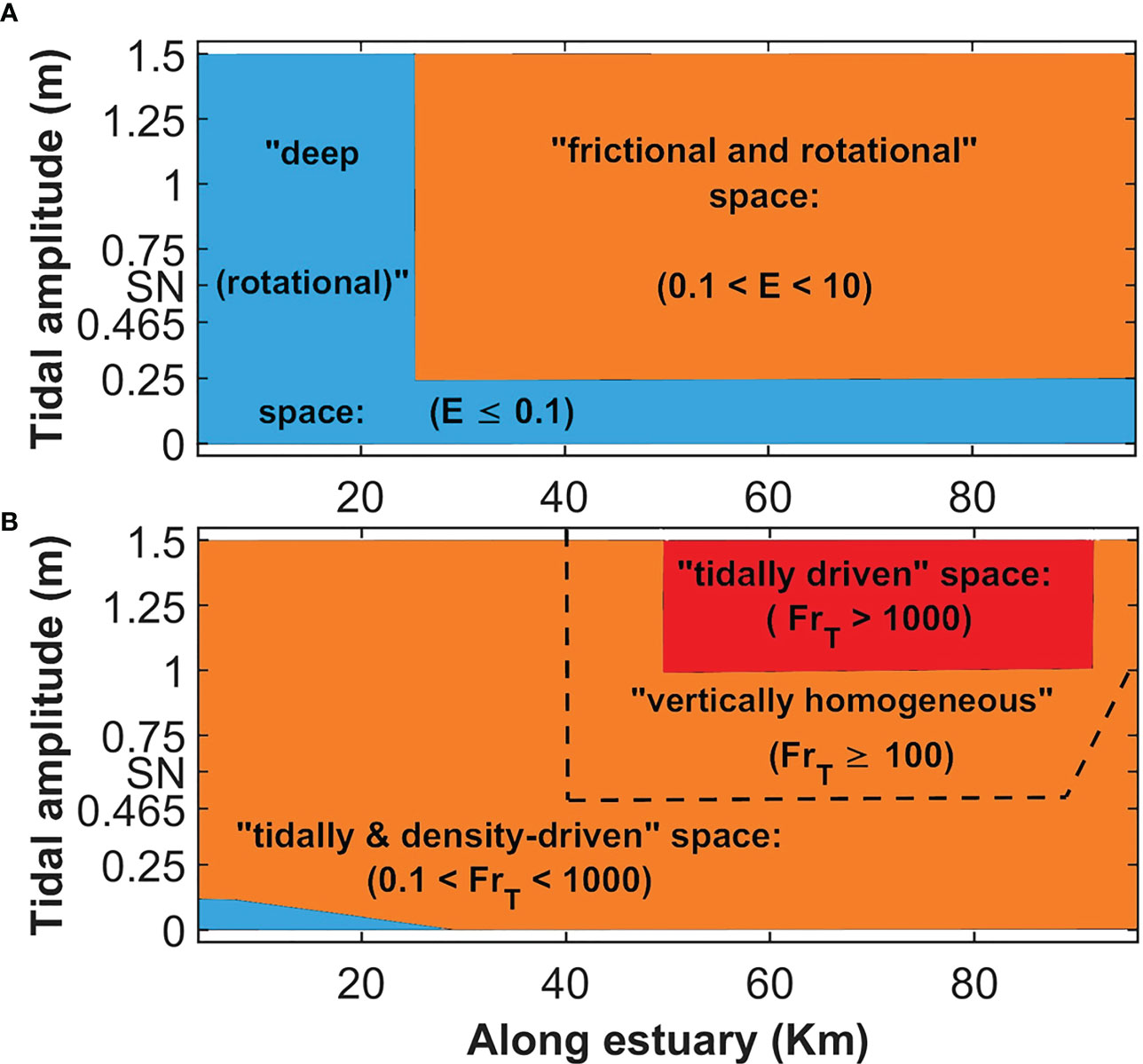
Figure 13 The schematic figures of the estuarine classification along the micro- and meso-tidal funnel-shaped salt-plug estuaries according to the longitudinal distributions of their Ekman (A) and tidal Froude numbers (B). “SN” on the y-axis stands for the spring-neap scenario of EXP11. The small blue color close to the estuary mouth (0 km-30 km) in (b) indicates “density-driven” space with $F{r}_T\le$ 0.1.

On the other hand, the micro-tidal salt-plug estuaries with tidal amplitudes lower than 0.25 have $F{r}_T$ values lower than 0.1 ($Log(F{r}_T)\le -1$), only close to the estuarine mouth that identifies “density-driven” classification. In the other words, almost none of the micro- and meso-tidal salt-plug estuaries (EXP4-EXP11) locate in the “density-driven” section.

According to the classification presented by (Valle-Levinson, 2021), the “tidally & density-driven” space with $-1<Log(F{r}_T)<1$ ($0.1<F{r}_T<10$) is only assigned to most of the inverse estuarine segments of the salt-plug estuaries with 0.25 m ≤ tidal amplitude ≤ 1 m and both inverse and positive segments of the estuaries with tidal amplitude< 0.25 m.

Also, based on this classification, the salinity maximum zone of the micro-tidal SPEs of EXP5, EXP6 and EXP11 (with tidal amplitude lower than 0.75 m) and the inverse estuarine segments of the meso-tidal EXP9 and EXP10 (with tidal amplitudes ≥ 1.25 m) belong to (“tidally driven” space) where $1<Log(F{r}_T)<2$ ($10<F{r}_T<100$). Although these areas and the salt plug of EXP 7 (with $Log(F{r}_T)~2.5$) are not completely “tidally driven” and they are also affected by density gradient (see Figures 7A, B).

On the other hand, the salinity maximum zones of the meso-tidal salt-plug estuaries of EXP8-EXP10 (with tidal amplitude ≥ 1m) have $Log(F{r}_T)\ge 3$ ($F{r}_T\ge 1000$) and correctly demonstrate a “tidally driven” section. Therefore, we suggest that the limitation of $0.1<F{r}_T<10$ for the “tidally & density-driven” section can change to $0.1<F{r}_T<1000$ and the “tidally driven” portion can be signified by $F{r}_T\ge 1000$ in salt-plug estuaries (see Figure 13B). Thus, both inverse and positive estuarine segments of meso-tidal salt-plug estuaries and almost all parts (inverse and positive segments and salt plug area) of micro-tidal salt-plug estuaries are located in “tidally & density-driven” space with $-1<Log(F{r}_T)<3$ ($0.1<F{r}_T<1000$).

Since the salt-plug estuaries mainly belong to the “tidally & density-driven” space (the orange color in Figure 13B), tidal straining can substantially modulate stratification conditions in these estuarine systems. In the framework proposed, the salinity maximum zone appears to possess special characteristics (like having peak values of tidal Froude and Ekman numbers and TKE coincidently) in the salt-plug estuaries, especially in the meso-tidal experiments. In this zone of the meso-tidal EXP8-EXP10 with salinity > 45 psu (Figure 7A), TKE > 0.001 m²/s² (Figure 7C), $Log(F{r}_T)>3$ (Figures 7B, 13B) and $Log(E)>0.25$ (Figures 9C, 13A), tidal forcing dominates density gradient so tide is the basic strong driver of the tidally averaged or residual flows.

In the zone with $F{r}_T\ge 100$ ($Log(F{r}_T)\ge 2$), the tidally averaged flow is weakly influenced by baroclinicity and can be labeled as “vertically homogeneous” in the framework for salt-plug estuaries (see Figures 7B, 13B). Although, (Valle-Levinson, 2021), presented the condition of $F{r}_T>10$ for the “vertically homogeneous” in the classification. The inverse estuarine segment of EXP2 (with 1m amplitude) is not vertically homogeneous (see Figures 8A, B) although the similar segment of EXP8 (with 1m amplitude) has $F{r}_T>10$ (see Figure 7B). In fact, the criteria of $F{r}_T\ge 100$ is consistent with the weakly stratified conditions within the salinity maximum zones in salt-plug estuaries with tidal amplitudes ≥ 0.5 m (see the mixed condition of EXP1 in Figure 2D), particularly in the meso-tidal EXP8-EXP10 (see Figure 7C), where $\acute{g}$ is almost minimal ($F{r}_T$ values are close to the maximum values), (see Figure 7B).

Valle-Levinson (2021) reported that the two transitions $E$ =1 and $F{r}_T=10$ may change from neap to spring tides and occur at different geographical locations at a specified time because of bathymetric variations, resulting in different $E$ and $F{r}_T$. In our study, the location of the salt plug in EXP11 (see Figure 7A) is close to both transition zones of $Log(E)~0$ (see Figure 9C) and $F{r}_T~100(Log(F{r}_T)~2)$ (see Figure 7B), which insignificantly changes from the neap to spring tides (see Figures 3C-F).

Conclusion

In this study, the hydrodynamics in micro- and meso-tidal salt-plug estuaries are investigated using the numerical model SCHISM. Several modeling experiments are performed using an idealized funnel-shaped basin, which is assumed to be located close to the Mond River Estuary in the Persian Gulf. This study addresses for the first time the competition between density gradients and tidal forcing in the formation of salt plugs, as well as their lateral circulation. The results show that the salt-plug estuary is characterized by a salinity maximum zone in the mid-estuary separating the inverse and positive estuarine subsystems. The salt plug shows weakly stratified conditions (high turbulent kinetic energy) and has high values of tidal Froude and Ekman numbers especially in the meso-tidal salt-plug estuaries. Increasing the tidal Froude number from the micro-tidal salt-plug estuaries (with tidal amplitudes less than 1 m at the estuary mouth) to the meso-tidal experiments (with tidal amplitudes higher than 1 m) results in a stronger salt plug with the tidal Froude number higher than 1000, extending from the mid-estuary to the head. It signifies dominating tidal forcing over baroclinicity in the strong salt plug and resulted from enhancing landward salt flux by tidal advection in the meso-tidal estuaries. The longitudinal and lateral circulations consequently change due to the resulting changes in the longitudinal salinity gradients. In the absence of Coriolis and wind forces, differential advection appears to be the dominant driver of lateral flows so that the time-averaged lateral circulations demonstrate very similar patterns (converging surface flows over the deep channel) within the positive and inverse subsystems. These lateral flows reverse in the area of the salt plug (diverging surface flows over the deep channel). Coriolis accelerations influence the lateral circulation driven by differential advection and lateral divergence dv/dy even at the narrow sections close to the head. In the salt-plug estuaries, tidal fluctuations in salinity show that maximum salinities occur at times of high water slacks in the upper positive estuarine segment and at low water slacks in the lower inverse segment, which impose the salinity cycle with approximately half the tidal period at the salt plug. This half-tidal period (the occurrence of maximum salinities during extreme tidal velocities) indicates the importance of salt transport by the tidal pumping process at the salt plug where the direction of tidal pumping of salt changes. The spring–neap variability in the salt-plug estuary shows that both longitudinal positive and inverse subtidal circulation cells join each other during neap tide and have a maximum distance in the mid-estuary (approximately 50 km) during spring tide. Also, the salt plug in the spring tide is slightly saltier than in the neap tide because of stronger tidal mixing and consequently a landward salt flux by tidal pumping during the spring tide contrary to the neap tide (with a seaward tidal salt flux) as well as a higher tidal advective salt flux in the spring tide. In addition, inside the salt plug, tidally averaged lateral circulations show downwelling cells in the spring tide and upwelling during the neap tide over the thalweg, indicating strong neap–spring variability. The salt plug location is controlled by the main longitudinal salt transports of tidal advection. Actually, this location is not considerably influenced by lateral flows. Although, the secondary flows can laterally redistribute isohalines in the vertical shape. For instance, the upwelling flows over the thalweg lift isohalines in the neap tide, while lying down lateral flows depress isohalines in the thalweg during the spring tide.

Data availability statement

The original contributions presented in the study are included in the article. Further inquiries can be directed to the corresponding authors.

Author contributions

STH, ES, JP and AVL contributed to the conception and design of the study. STH and JP developed the model set-up and different numerical experiments. STH performed model analyses and wrote the first draft of the manuscript. ES, AVL, and CS advised on the analysis of model results. All authors contributed to the article and approved the submitted version.

Funding

This study is a contribution to theme “C3: Sustainable Adaption Scenarios for Coastal Systems” of the Cluster of Excellence EXC 2037 ‘CLICCS - Climate, Climatic Change, and Society’ – Project Number: 390683824 funded by the Deutsche Forschungsgemeinschaft (DFG, German Research Foundation) under Germany’s Excellence Strategy.

Acknowledgments

This study used data from the DHI, CMEMS and ECMWF. Additionally, we thank Benjamin Jacob (Helmholtz-Zentrum Hereon) for his help with modeling.

Conflict of interest

The authors declare that the research was conducted in the absence of any commercial or financial relationships that could be construed as a potential conflict of interest.

Publisher’s note

All claims expressed in this article are solely those of the authors and do not necessarily represent those of their affiliated organizations, or those of the publisher, the editors and the reviewers. Any product that may be evaluated in this article, or claim that may be made by its manufacturer, is not guaranteed or endorsed by the publisher.

References

Aristizábal MaríaF., Chant R. J. (2015). An observational study of salt fluxes in Delaware bay. J. Geophys. Res.: Oceans 120 (4), 2751–2768. doi: 10.1002/2014JC010680

CrossRef Full Text | Google Scholar

Cabrera O. C., Villanoy C. L., Jacinto G. S., Bernardo L. P. C., Ferrera C. M., Velasquez I. B., et al. (2014). Salt-plug estuarine circulation in malampaya sound, palawan, Philippines. Phil. Sci. Lett. 7, 428–437.

Google Scholar

Chant R. J. (2010). “Estuarine secondary circulation,” in Contemporary issues in estuarine physics (Cambridge University Press), 100–124. doi: 10.1017/CBO9780511676567.006

CrossRef Full Text | Google Scholar

Chen S.-N., Sanford L. P. (2009). Lateral circulation driven by boundary mixing and the associated transport of sediments in idealized partially mixed estuaries. Continental Shelf Res. 29 (1), 101–118. doi: 10.1016/j.csr.2008.01.001

CrossRef Full Text | Google Scholar

Cheng Y., Andersen O. B. (2010). Improvement in global ocean tide model in shallow water regions. Poster SV 45, 1–68.

Google Scholar

Ensing E., de Swart H. E., Schuttelaars H. M. (2015). Sensitivity of tidal motion in well-mixed estuaries to cross-sectional shape, deepening, and sea level rise. Ocean Dynam. 65 (7), 933–950. doi: 10.1007/s10236-015-0844-8

CrossRef Full Text | Google Scholar

Friedrichs C. T. (2010). Barotropic tides in channelized estuaries. Contemp. Issues Estuar. Phys. 27, 61. doi: 10.1017/CBO9780511676567.004

CrossRef Full Text | Google Scholar

Friedrichs C. T., Valle-Levinson A. (1998). Transverse circulation associated with lateral shear in tidal estuaries. Proceedings, Physics of Estuaries and Coastal Seas, 9th International Biennial Conference, Sponsored by Kyushu and Ehime Universities, Matsuyama, Japan, 24-26 September, p. 15–17.

Google Scholar

Garvine R. W. (1995). A dynamical system for classifying buoyant coastal discharges. Continental Shelf Res. 15 (13), 1585–1596. doi: 10.1016/0278-4343(94)00065-U

CrossRef Full Text | Google Scholar

Geyer W.R. (1993). Three-dimensional tidal flow around headlands. J. Geophys. Res.: Oceans 98 (C1), 955–966. doi: 10.1029/92JC02270

CrossRef Full Text | Google Scholar

Geyer W.R., MacCready P. (2014). The estuarine circulation. Annu. Rev. fluid mechanics 46, 175–197. doi: 10.1146/annurev-fluid-010313-141302

CrossRef Full Text | Google Scholar

Ghaemi M., Gholamipour S. (2017). Seasonal measurement of nutrient concentrations and total alkalinity in the mond estuary ecosystem. J. Oceanogr. 8 (30), 11–18. doi: 10.29252/joc.8.30.11

CrossRef Full Text | Google Scholar

Hosseini S. T., Chegini V., Sadrinasab M., Siadatmousavi S. M., Yari S. (2016). Tidal asymmetry in a tidal creek with mixed mainly semidiurnal tide, bushehr port, Persian gulf. Ocean Sci. J. 51 (2), 195–208. doi: 10.1007/s12601-016-0017-9

CrossRef Full Text | Google Scholar

Hosseini S. T., Siadatmousavi S. M. (2018). Field observations of hypersaline runoff through a shallow estuary. Estuarine Coast. Shelf Sci. 202, 54–68. doi: 10.1016/j.ecss.2017.12.003

CrossRef Full Text | Google Scholar

Huijts K. M. H., de Swart H. E., Schramkowski G. P., Schuttelaars H. M. (2011). Transverse structure of tidal and residual flow and sediment concentration in estuaries. Ocean Dynam. 61 (8), 1067–1091. doi: 10.1007/s10236-011-0414-7

CrossRef Full Text | Google Scholar

Johnson G. C., Ohlsen D. R. (1994). Frictionally modified rotating hydraulic channel exchange and ocean outflows. J. Phys. Oceanogr. 24 (1), 66–78. doi: 10.1175/1520-0485(1994)024<0066:FMRHCE>2.0.CO;2

CrossRef Full Text | Google Scholar

Juarez B., Valle-Levinson A., Li C. (2020). Estuarine salt-plug induced by freshwater pulses from the inner shelf. Estuarine Coast. Shelf Sci. 232, 106491. doi: 10.1016/j.ecss.2019.106491

CrossRef Full Text | Google Scholar

Khosravi M., Siadatmousavi S. M., Vennell R., Chegini V. (2018). The transverse dynamics of flow in a tidal channel within a greater strait. Ocean Dynam. 68 (2), 239–254. doi: 10.1007/s10236-017-1127-3

CrossRef Full Text | Google Scholar

Kranenburg W. M., Geyer W.R., Garcia A. M. P., Ralston D. K. (2019). Reversed lateral circulation in a sharp estuarine bend with weak stratification. J. Phys. Oceanogr. 49 (6), 1619–1637. doi: 10.1175/JPO-D-18-0175.1

CrossRef Full Text | Google Scholar

Largier J. (2010). “Low-inflow estuaries: hypersaline, inverse, and thermal scenarios” in Contemporary issues in estuarine physics. (Cambridge: Cambridge University Press), 247–272. doi: 10.1017/CBO9780511676567

CrossRef Full Text | Google Scholar

Lerczak J. A., Geyer W.R. (2004). Modeling the lateral circulation in straight, stratified estuaries. J. Phys. Oceanogr. 34 (6), 1410–1428. doi: 10.1175/1520-0485(2004)034<1410:MTLCIS>2.0.CO;2

CrossRef Full Text | Google Scholar

Lerczak J. A., Geyer W.R., Chant R. J. (2006). Mechanisms driving the time-dependent salt flux in a partially stratified estuary. J. J. Phys. Oceanogr. 36 (12), 2296–2311. doi: 10.1175/JPO2959.1

CrossRef Full Text | Google Scholar

Li M., Cheng P., Chant R., Valle-Levinson A., Arnott K. (2014). Analysis of vortex dynamics of lateral circulation in a straight tidal estuary. J. Phys. Oceanogr. 44 (10), 2779–2795. doi: 10.1175/JPO-D-13-0212.1

CrossRef Full Text | Google Scholar

Li C., O’Donnell J. (1997). Tidally driven residual circulation in shallow estuaries with lateral depth variation. J. Geophys. Res.: Oceans 102 (C13), 27915–27929. doi: 10.1029/97JC02330

CrossRef Full Text | Google Scholar

Li C., Valle-Levinson A. (1999). A two-dimensional analytic tidal model for a narrow estuary of arbitrary lateral depth variation: the intratidal motion. J. Geophys. Res.: Oceans 104 (C10), 23525–23543.

Google Scholar

Mariani R., Lessa G. C., Marta-Almeida M. (2022). Long-term variability of the salinity field in a Large tropical, well-mixed estuary: the influence of climatic trends. Estuaries Coasts 45 (3), 721–736. doi: 10.1007/s12237-021-01008-y

CrossRef Full Text | Google Scholar

Nunes R. A., Simpson J. H. (1985). Axial convergence in a well-mixed estuary. Estuarine Coast. Shelf Sci. 20 (5), 637–649. doi: 10.1016/0272-7714(85)90112-X

CrossRef Full Text | Google Scholar

Ott M. W., Garrett C. (1998). Frictional estuarine flow in Juan de fuca strait, with implications for secondary circulation. J. Geophys. Res.: Oceans 103 (C8), 15657–15666. doi: 10.1029/98JC00019

CrossRef Full Text | Google Scholar

Pein J., Valle-Levinson A., Stanev E. V. (2018). Secondary circulation asymmetry in a meandering, partially stratified estuary. J. Geophys. Res.: Oceans 123 (3), 1670–1683. doi: 10.1002/2016JC012623

CrossRef Full Text | Google Scholar

Phillips O. M. (1970). On flows induced by diffusion in a stably stratified fluid. Deep Sea Res. Oceanogr Abstracts. 17, 435–443. doi: 10.1016/0011-7471(70)90058-6

CrossRef Full Text | Google Scholar

Rozovskii I. L. (1957). “Flow of water in bendsof open channels.” The Academy of Science of the Ukraine SSR. SUKEQAWA, N. 1971 Conditions for the occurrence of river meanders. Trans. JSCE 2, 257–261.

Google Scholar

Scully M. E., Geyer W.R., Lerczak J. A. (2009). The influence of lateral advection on the residual estuarine circulation: a numerical modeling study of the Hudson river estuary. J. Phys. Oceanogr. 39 (1), 107–124. doi: 10.1175/2008JPO3952.1

CrossRef Full Text | Google Scholar

Shaha D. C., Cho Y.-K. (2016). Salt plug formation caused by decreased river discharge in a multi-channel estuary. Sci. Rep. 6 (1), 1–11. doi: 10.1038/srep27176

PubMed Abstract | CrossRef Full Text | Google Scholar

Stanev E. V., Jacob B., Pein J. (2019). German Bight estuaries: an inter-comparison on the basis of numerical modeling. Continental Shelf Res. 174, 48–65. doi: 10.1016/j.csr.2019.01.001

CrossRef Full Text | Google Scholar

Umlauf L., Burchard H. (2003). A generic length-scale equation for geophysical turbulence models. J. Mar. Res. 61 (2), 235–265. doi: 10.1357/002224003322005087

CrossRef Full Text | Google Scholar

Valle-Levinson A. (2008). Density-driven exchange flow in terms of the kelvin and ekman numbers. J. Geophys. Res.: Oceans 113, C04001. doi: 10.1029/2007JC004144

CrossRef Full Text | Google Scholar

Valle-Levinson A. (2010). Definition and classification of estuaries. In Valle-Levinson A. (Ed.), Contemporary Issues in estuarine physics (pp. 1–11). Cambridge, UK: Cambridge University Press. doi: 10.1017/CBO9780511676567.002

CrossRef Full Text | Google Scholar

Valle-Levinson A. (2011). 1.05 classification of estuarine circulation. Treatise Estuar. Coast. Sci. 1, 75–86. doi: 10.1016/B978-0-12-374711-2.00106-6

CrossRef Full Text | Google Scholar

Valle-Levinson A. (2021). Dynamics-based classification of semienclosed basins. Regional Stud. Mar. Sci. 46, 101866. doi: 10.1016/j.rsma.2021.101866

CrossRef Full Text | Google Scholar

Valle-Levinson A. (2022). Introduction to estuarine hydrodynamics (Cambridge University Press). doi: 10.1017/9781108974240

CrossRef Full Text | Google Scholar

Valle-Levinson A., Bosley K. T. (2003). Reversing circulation patterns in a tropical estuary. J. Geophys. Res.: Oceans 108 (C10), 3331. doi: 10.1029/2003JC001786

CrossRef Full Text | Google Scholar

Valle-Levinson A., Reyes C., Sanay R. (2003). Effects of bathymetry, friction, and rotation on estuary–ocean exchange. J. Phys. Oceanogr. 33 (11), 2375–2393. doi: 10.1175/1520-0485(2003)033<2375:EOBFAR>2.0.CO;2

CrossRef Full Text | Google Scholar

Wolanski E. (1986). An evaporation-driven salinity maximum zone in Australian tropical estuaries. Estuarine Coast. Shelf Sci. 22 (4), 415–424. doi: 10.1016/0272-7714(86)90065-X

CrossRef Full Text | Google Scholar

Wunsch C. (1970). On oceanic boundary mixing. Deep Sea Res Oceanogr. Abstracts 17, 293–301. doi: 10.1016/0011-7471(70)90022-7

CrossRef Full Text | Google Scholar

Zhang Y. J., Ye F., Stanev E. V., Grashorn S. (2016). Seamless cross-scale modeling with SCHISM. Ocean Model. 102, 64–81. doi: 10.1016/j.ocemod.2016.05.002

CrossRef Full Text | Google Scholar