Assessment of predictability of the Loop Current in the Gulf of Mexico from observing system experiments and observing system simulation experiments

1 Introduction

The Gulf of Mexico (GoM) marine basin provides significant economic, ecological, and biological value. The Gulf provides 15% of the total U.S. domestic oil and 1% of natural gas production (Zeringue et al., 2022) with over 3,200 active oil and gas structures (NOAA NCEI Gulf of Mexico Data Atlas, https://www.ncei.noaa.gov/maps/gulf-data-atlas/atlas.htm?plate=Offshore%20Structures, accessed 23 January 2023). Accurate and timely forecasts of strong currents associated with the energetic mesoscale features such as the Loop Current (LC) and Loop Current eddies (LCEs) at the offshore production sites are of great importance for oil and gas operations. Improved understanding and predictive capabilities of the LC system have also major implications for hurricane forecasts (Shay et al., 2000), oil spill response and preparedness (Walker et al., 2011; Weisberg et al., 2017), biogeochemical variability (Damien et al., 2021), sustainability of fisheries (Weisberg et al., 2014; Selph et al., 2022), and forecasting sargassum transport and harmful algal blooms (Gower and King, 2011; Liu et al., 2016). The necessity of improved predictability of the LC system from short-range (from a few days to a week) to long-range (3 months and longer) has been emphasized in a call to action by the National Academies of Sciences, Engineering, and Medicine (NASEM, 2018). The importance of this problem has motivated the Understanding Gulf Ocean Systems (UGOS) research initiative (part of the NASEM Gulf Research Program) focused on improving our knowledge and forecasts of the GoM circulation in spatial and time scales useful for a broad community of stakeholders.

A modeling research project conducted by a consortium of university researchers funded by UGOS Phase 1 (UGOS-1) has the overarching goal to achieve greater understanding of the physical processes that control the LC and LCE separation dynamics through advanced data-assimilative modeling and analyses. One of the objectives of the study is to examine the limits of predictability of the LC system using multi-model forward simulations. Several modeling groups conducted coordinated experiments using different data-assimilative modeling systems to test the performance and sensitivity of existing Gulf of Mexico forecasting models and to evaluate long-range prediction capabilities. The numerical experiments included Observing System Experiments (OSEs) and Observing System Simulation Experiments (OSSEs). OSEs apply existing observational data to evaluate the sensitivity of a data assimilative system to different types of observations and their combination (Fujii et al., 2019). In OSSEs, synthetic observations derived from a realistic simulation (“nature run”) are used as constraints in data assimilation systems (Lahoz and Schneider, 2014).

The predictability of a model can be defined as the time extent within which the true state can be predicted within some finite error (e.g., Lorenz, 1965; Lorenz, 1984; Krishnamurthy, 2019). Many metrics have been employed to measure the predictability (e.g., DelSole, 2004; Krause et al., 2005). In most studies, the predictability is evaluated based on the square error or mean square error between the predicted state and truth (Lorenz, 1965; Lorenz, 1984; Dalcher and Kalnay, 1987; Oey et al., 2005). The error-based measure of predictability follows a mathematical theory of the growth of initial errors formulated by Lorenz (1965). According to this theory, the error of the forecast increases with lead-time. The amplification factor of the error is not constant and depends on the model parameters, the initial magnitude of the error, as well as the system itself. Typically, forecast error growth rate is largest at the beginning and then the magnitude of the forecast error levels off, asymptotically approaching the limiting value, called the saturation value. The saturation value is comparable to the expected error of two randomly chosen states of the system (Lorenz, 1965; Dalcher and Kalnay, 1987). This means that when the forecast error approaches the saturation value, its predictive skill is no better than any randomly selected state of the system. The time taken to reach the saturation level has been used as a measure of the predictability of forecasting systems (DelSole, 2004; Krishnamurthy, 2019). Another measure of the model predictability used in atmospheric forecasts is the doubling time of the errors (e.g., Charney et al., 1966; Lorenz, 1982). However, it has been shown that this parameter is not a good measure of error growth and predictability (e.g., Dalcher and Kalnay, 1987).

Some studies compare statistics derived from forecasts and reference states to evaluate model predictive skill. For example, Thoppil et al. (2021) compared RMSE computed from forecasts and from a monthly mean climatology of ocean observations. This work defined that the model has predictive skills if RMSE is lower than RMSE from climatology data. In other studies, the predictability is measured in terms of time when cross-correlation between the forecast and observations drops below a threshold value (e.g., Latif et al., 1998). Boer (2000) used cumulative scaled predictability statistics derived from cross-correlation between the forecast and observations to investigate the predictability of the coupled atmosphere-ocean system on time scales of monthly to decadal. The statistics were compared against threshold values to evaluate model predictability. Many skill scores are referenced with respect to persistence prediction or persistence (Mittermaier, 2008). Alternatively, predictive skill scores can be referenced with respect to a random forecast (Wilks, 2006) or climatology (DelSole, 2004).

The type of predicted characteristics selected for evaluation of the predictability dictates the choice of the metrics. In the GoM, the shape and location of the LC and LCEs are the main predicted characteristics. The model prediction skill assessment is performed by comparing the LC/LCE frontal positions in the forecast and control data set. In many studies, the LC/LCE fronts are defined from the sea surface height (SSH) fields using a threshold value (e.g., 0.17 m in Leben, 2005; 0.45 m in Zeng et al., 2015). Oey et al. (2005) defined forecast frontal positions by contouring the 18°C isotherm at 200 m. Dukhovskoy et al. (2015a) used SSH gradient field to correct the first guess of the LC frontal position derived from the SSH 0.17 m contour. Comparison of the contours or shapes requires special metrics providing robust error estimates that measure dissimilarity of the objects. Oey et al. (2005) used shortest distance from the LC/LCE fronts to several locations in the Gulf derived from the forecasts and observations to deduce the forecast error in frontal position. This metric may provide an acceptable measure of the model forecast skill for the predicted characteristic defined as the shortest distance from the LC/LCE front to specific locations. However, it does not provide information about the shape of the LC front. In theory, there are an infinite number of possible LC/LCE shapes that will have identical distances to the specified locations. To address this, Dukhovskoy et al. (2015b) tested five metrics for contour and shape comparison and demonstrated that the Modified Hausdorff Distance (MHD) method (Dubuisson and Jain, 1994) exhibits high skill and robustness in quantifying similarity between the objects. This metric has been successfully applied for evaluation of model skill for simulating river plumes (Hiester et al., 2016). There are other methods specifically designed for contour comparison in geophysical applications that could potentially be applied for LC/LCE frontal position skill assessment (Goessling and Jung, 2018; Melsom et al., 2019).

For most of the documented GoM forecast systems, predictability of the LC position is approximately 3–5 weeks (Oey et al., 2005; Mooers et al., 2012). Forecasting a LCE separation event is a challenging prediction task for GoM circulation models and its predictability is on the order of a month (Mooers et al., 2012). It should be noted that predictability estimates from other model studies are not comparable when different measures of predictability, predicted characteristics, reference state, and type of control data sets are used. Also, predictability characterizes predictive skills of the particular model used for prediction and does not describe the predictability of the process being forecast, although, the process determines the time scale of the model predictability (Krishnamurthy, 2019).

This paper summarizes results of numerical experiments performed using a high-resolution (~2.5 km) regional data-assimilative system to systematically assess the impact of different types of observations on the predictive time scale in the GoM. To evaluate the impact of specific observations (SSH, temperature (T) and salinity (S) profiles, etc.) on the predictive skills of the forecasting system, we perform free-running (no data assimilation) forecasts initialized from the runs that assimilate real observations (OSEs) and synthetic observations derived from a high-resolution independent simulation (OSSEs). Results of the OSEs and OSSEs demonstrate the importance of minimizing the error in the forecast initial fields for accurate forecasts. In its turn, the accuracy of the hindcasts providing initial fields depend on availability of observations and assimilation techniques.

The layout of the paper is as follows. Section 2 describes the data-assimilative system and the methods for model skill assessment. Then, results of the OSEs using various combinations of observations are presented in section 3. In section 4, we use OSSEs and a nature run to further assess the predictability of the forecasting system. Finally, the results are discussed and summarized in section 5.

2 Model configuration, nature run, and metrics

2.1 The 1/32.5° intra-American seas HYCOM-TSIS

A regional configuration of the HYbrid Coordinate Ocean Model (HYCOM; Bleck, 2002; Chassignet et al., 2003; Halliwell, 2004) is used for the data-assimilative OSEs and OSSEs. The computational grid has uniform 1/32.5° horizontal spacing (~2.5 km) between 98.08°W and 56.08°W and 7.03°N and 31.93°N (Figure 1). The Intra-American seas (IAS HYCOM) domain includes the GoM and the Caribbean Sea. This configuration keeps the open boundaries away from the Gulf reducing the boundary effect on the numerical solution in the GoM, which is the study region. The model bathymetry is a combination of global 1-arc-min ocean depth and land elevation from the U.S. National Geophysical Data Center (ETOPO1; https://www.ngdc.noaa.gov) and the 15-arc-second General Bathymetric Chart of the Oceans (GEBCO; https://www.gebco.net/data_and_products/gridded_bathymetry_data/) 2020 grid with local corrections in the Gulf of Mexico. The model employs 30 vertical hybrid layers with potential densities referenced to 2000 db and ranging from 27.10 to 37.17 sigma units. The model is forced with NCEP CFSR and CFSv2 atmospheric fields of air temperature and specific humidity at 2 m, surface net short- and long-wave radiation, precipitation, and 10 m wind stress. Monthly climatological river discharge is prescribed at all major rivers resulting in a negative salt flux at the river sources. A combination of Laplacian and biharmonic mixing is used for horizontal momentum diffusion. The mixing is specified in terms of diffusion velocity, that is 2.86×10^-3 m s^-1 for Laplacian momentum dissipation, 5.0×10^-3 m s^-1 for scalar diffusivity, and 0.01 m s^-1 for biharmonic momentum dissipation and layer thickness diffusivity. The K-profile parameterization (KPP; Large et al., 1994) is used for vertical mixing with default values.

FIGURE 1

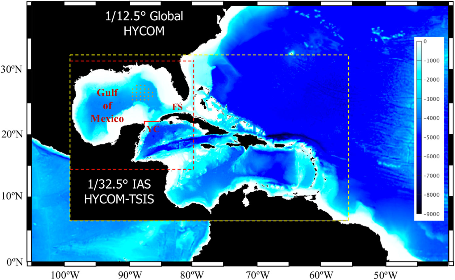
Figure 1 Bathymetry map of the computational domain of the 1/32.5° IAS HYCOM-TSIS forecast modeling system (yellow dashed box) nested within the outer model. In OSEs, the domain is nested into the 1/12.5° Global HYCOM reanalysis (GOFS3.0). In OSSEs, the domain is nested into the 1/12° GLORYS reanalysis. The red dashed lines delineate the outer boundaries of the NEMO domain providing the nature run fields. The orange bullets in the eastern GoM indicate PIES locations. The Yucatan Channel (YC) and the Florida Straits (FS) are indicated. The red line designates location of the vertical section of the mean along-channel velocities shown in Figure 4.

For data assimilation of the observations in HYCOM, we use the Tendral Statistical Interpolation System (T-SIS) version 2.0. The interpolation algorithm is based on the Kalman filtering approach with a novel technique for solving the least squares normal equations. The suggested solution uses the information matrix (inverse of the covariance matrix), which significantly reduces computational complexity of calculation of the filter gain matrix. Details of the parameterization of the inverse covariance using Markov random fields are in Srinivasan et al. (2022). In the numerical experiments presented here, different types of oceanographic fields are assimilated as discussed in sections 3 and 4 (OSEs and OSSEs, respectively). All experiments consist of data-assimilative hindcasts simulations (analysis) followed by 3-month free-running forecasts initialized from the analysis fields at specified times.

2.2 OSSE nature run

In the OSSE hindcasts (section 4), synthetic observations, derived from another simulation, the so-called nature run (NR), are assimilated in the forecasting system. The NR model is chosen to perform the most statistically realistic simulation of the ocean as possible. The NR should be an unconstrained simulation performed at high resolution using a state-of-the-art general circulation model. For OSSEs to be credible, it is essential that the NR provides the most accurate possible representation of the true system, that is, possess a model climatology and variability with statistical properties that agree with observations to within specified limits. Here, the NR solution is provided by a GoM simulation performed with the Nucleus for European Modeling of the Ocean program (NEMO.4.0; Madec et al., 2017) ocean model at Centro de Investigación Científica y de Educación Superior de Ensenada (CICESE, Mexico). This model is configured on a 1/108° horizontal grid (~900 m spatial grid spacing) with 75 vertical levels. The model domain is shown in Figure 1 with the dashed red lines. The NR is initialized from the 1/12° GLORYS12 global reanalysis (Lellouche et al, 2021) and is integrated using boundary (surface and lateral) forcing and no assimilation for the period from 1 January 2009 to 31 December 2014. The lateral boundary conditions are derived from the GLORYS12 reanalysis. At the surface, the atmospheric fluxes of momentum, heat and freshwater are computed by bulk formulae using the COARE 3.5 algorithm (Edson et al., 2013). The model is forced with the Drakkar Forcing Field (DFS5.2) atmospheric fields product (Dussin et al., 2016) which is based on the ERA-interim reanalysis and consists of 3-hour fields of wind, atmospheric temperature and humidity, atmospheric pressure at the sea level, and daily fields of long, short wave radiation and precipitation.

2.3 Metrics, forecast predictability, and skill assessment

The performance of the data-assimilative runs and forecasts is assessed by two metrics: the root mean square error (RMSE) and the MHD. Both metrics quantify the disagreement between the forecast and the true state and can be used as a measure of predictability and skill assessment of the model simulation.

2.3.1 The root mean square error

The RMSE is computed to quantify the difference between spatial distributions of a scalar field from the simulation and the control run, and is computed as

$\begin{array}{ll}{E}_{RMSE}=\left(\frac{{\sum }_{i=1}^n{(x_i-{\tilde{x}}_i)}^2}{N}\right)1/2,& (1)\end{array}$

where x_i is scalar value at the i^th point in the simulation and ${\tilde{x}}_i$ is the value at the corresponding point from the control data field. The comparison is performed for spatial fields; in this case, i is the grid point index. The RMSE provides a quantitative estimate of the overall agreement between two fields (a forecast and a control field) based on a statistical score (eq. 1). However, for the purposes of this study, more precise assessment of a model run was needed to evaluate the model skill in predicting the LC system in terms of the LC position and shape; therefore, a topological metric, the MHD, is also employed.

2.3.2 Modified Hausdorff distance of the loop current front

There are two steps in this skill assessment approach. First, the contours representing the LC and LCE fronts are derived from the SSH fields of a tested simulation and control data (e.g., control model run, altimetry gridded data) following Leben (2005) and Dukhovskoy et al. (2015a). Second, the MHD score ($D_{MHD}$) is computed for the two contours considered as sets of points (A and B)

$\begin{array}{ll}{D}_{MHD}(A,B)\equiv max\left\{\frac{1}{\left|A\right|}{\sum }_{a\in A}d(a,B),\frac{1}{\left|B\right|}{\sum }_{b\in B}d(A,b)\right\},& (2)\end{array}$

where |A| and |B| are the cardinality of sets A and B, $d(a,B)\equiv \underset{b\in B}{\min }d(a,b)$ and $d(A,b)\equiv \underset{a\in A}{\min }d(a,b)$. Next, the MHD scores are used for evaluating the predictability skills of the forecast compared to control data. Identical LC frontal positions result in zero MHD. The MHD score increases as the two contours (i.e., the LC frontal positions) become more dissimilar. The MHD units depend on the positional units or can be unitless (normalized distances, for instance). Here, MHD is in km for ease of interpretation.

While MHD is a robust objective metric, measuring dissimilarities in two-dimensional and which can be generalized to N-dimensional fields (Dukhovskoy et al., 2015b), different definitions of the LC front may result in different contours impacting the MHD score and model skill assessment. This is particularly true during LCE detachment and reattachment when the LC shape drastically changes within several hours. As an illustration, the daily mean SSH fields from the NEMO NR and one of the HYCOM OSSE forecasts are shown for two consecutive dates (Figure 2). The LC front is defined using the 17-cm contour of demeaned SSH shown with the red lines in the upper and middle panels. The bottom panels show the two contours representing the LC fronts from the control field (NR) and the forecast and the MHD score is computed for these contours. At the end of the 3-month HYCOM forecast, the LC shapes from the NR truth and the forecast are notably dissimilar. Yet, there is some agreement in the positioning and size of the LC on April 9, 2012. Between April 9 and the following day, the LC sheds an eddy in the forecast, but not in the NR (Figure 2B). If one were to adopt a definition of the contours that only include the LC, this would result in a drastic increase of the MHD score (or decrease in the prediction skill) for the forecast because the LC is in the retracted position whereas it is in the extended position in the NR. In many cases, a LCE reattaches the LC several days later now causing a sudden decrease in the MHD score. In this study, the prediction skill is assessed for the whole LC system that includes LCEs that are within a certain distance to the LC (somewhat similar to Oey et al., 2005). The definition of the predicted characteristics would be different if the predictability of the shedding event were the main focus of this study.

FIGURE 2

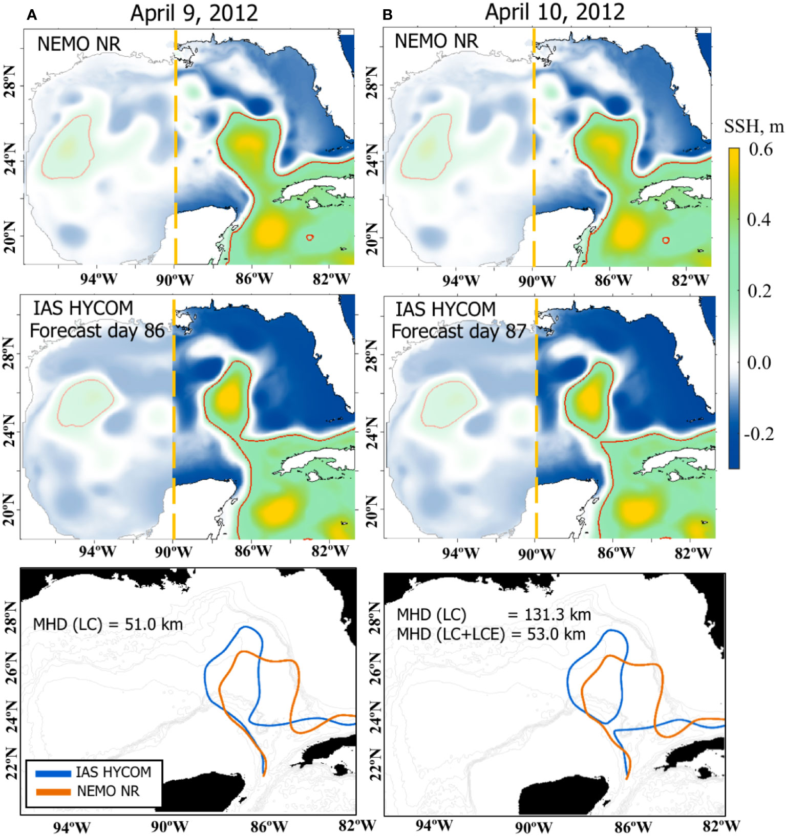
Figure 2 The SSH fields and the LC/LCE fronts from the NEMO NR (top row) and one of the 1/32.5° IAS HYCOM OSSE forecasts (middle) for April 9, 2012 (left column, A) and April 10, 2012 (right column, B). The red lines indicate LC/LCE fronts defined as the 17-cm contours of the demeaned SSH. The bottom panels show the LC/LCE fronts used for the MHD calculation with the MHD score listed. For the NR, only LCEs that are in the east of 90°W are considered for the MHD (the eddies that are in the shaded area are ignored). For (B), the two MHD scores of the forecast (blue) are given: for the LC front only and the LC with the LCE fronts combined.

To mitigate the impact of LCE detachment and reattachment on the MHD score, keeping in mind that the focus of the experiment is on the frontal locations for the entire LC system (including eddies) rather than the timing of the LCE shedding, the following approach is used to define the fronts for MHD skill assessment. An automated algorithm tracks the LC and LCEs in the SSH fields similar to Dukhovskoy et al. (2015a). LCEs west of 90°W are discarded (shaded region in Figure 2). For other LCEs, the MHD is computed for all possible combinations of the LCEs (including none) with the LC both for the forecast and the control fields. Then the best (smallest) MHD score is selected. For the case presented in Figure 2B, the combination of the LCE contour with the LC from the forecast yields a smaller MHD score than for the LC alone (53 vs 131.3 km) and, therefore, both the LCE and LC contours from the forecast versus the LC contour from the control field are used for MHD.

2.3.3 Assessment of predictability

As mentioned above, two metrics, RMSE and MHD, are used to evaluate the model predictability. The predictability is considered to be lost when the RMSE is comparable to the saturation value. Sensitivity testing of the MHD metric conducted by Dukhovskoy et al. (2015b) demonstrated that the MHD linearly responds to the linearly increasing error in the shape. Therefore, the idea of saturation value is also applicable to the MHD metric meaning that the MHD score will increase as the dissimilarity between the forecast and the control frontal position, due to forecast error, increases approaching the saturation value. Note that an agreement between the RMSE and MHD scores is expected, however the MHD evaluates only the LC and LCE shapes, whereas RMSE provides a spatially average score for the whole GoM and is less sensitive to mismatch in the LC frontal position in the forecast and the control data.

In order to assess predictability of the forecast system, RMSE and MHD scores are compared against the saturation values. The estimates of the RMSE saturation value ($RMS{E}_{\infty }$) and MHD saturation value ($MH{D}_{\infty }$) are derived from the SSH fields of the NEMO NR for 2010 and 2012 (Figure 3). The randomly selected fields are at least 90 days apart from each other to avoid similar states of the SSH. The distributions of $RMS{E}_{\infty }$ and $MH{D}_{\infty }$ are symmetric and close to normal with similar mean and median. Following Dalcher and Kalnay (1987), 95% of the estimated saturation values ($RMS{E}_{\infty }=$ 0.178 m and $MH{D}_{\infty }=$ 66.3 km) are used in our analysis of the forecast experiments for predictability assessment. The estimated $RMS{E}_{\infty }$ agrees well with that of Zeng et al. (2015) who used a threshold value of 0.7 for spatial correlation coefficients of predicted and observed SSH to evaluate prediction skill of the forecasts. According to Zeng et al. (2015), the spatial RMSE of SSH exceeded $RMS{E}_{\infty }$ for the forecasts with spatial correlation <0.7 (Figure 3 in Zeng et al., 2015).

FIGURE 3

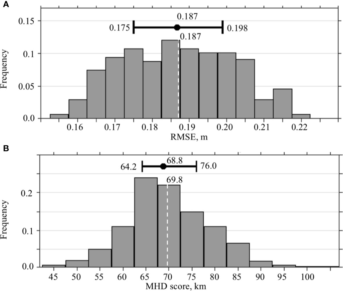
Figure 3 Statistics of the RMSE and MHD scores characterizing the saturation value. (A) Distribution of the RMSE between two randomly selected SSH fields form the NEMO NR. (B) Distribution of the MHD scores calculated for the LC/LCE fronts derived from randomly selected SSH fields from the NEMO NR. At the upper part of the diagrams, the median and IQR with the values are shown. The dashed white line is the expected value with the value listed at the top.

Model forecast skill is defined as forecast performance relative to the performance of a reference forecast demonstrating added value of the forecast (Mittermaier, 2008). If the state of the system at time t is X(t), where $X\in {ℝ}^n$, then persistence prediction at lead time $\tau$ is$X(t+\tau )=X(t)$. In our case, persistence is the initial fields of the forecast simulation. Persistence is a useful comparison of the model skill that provides measure of added value relative to some benchmark. However, no conclusion on predictability of the forecast system can be usually drawn from this. Also, skill assessment depends on the choice of the benchmark as a reference state (Niraula and Goessling, 2021).

3 Observing system experiments

In this first series of the experiments (OSEs), the IAS HYCOM is nested within the 1/12.5° global HYCOM reanalysis GOFS3.0 (Metzger et al., 2014) and hindcasts of the GoM state during the time period from 2009 through 2011 are performed using observational data for constraining the numerical solution used for the forecasts. The OSEs assimilate sea level anomaly (SLA) derived from the satellite altimetry observations (AVISO L3 along-track data downloaded from https://www.aviso.altimetry.fr/en/data/products/sea-surface-height-products/global.html), gridded sea surface temperature (SST) fields provided by the Group for High Resolution Sea Surface Temperature (GHRSST, downloaded from https://www.ghrsst.org), and temperature and salinity profiles derived from Argo floats (downloaded from https://usgodae.org/argo/argo.html) and pressure inverted echo sounders (PIES, available at http://www.po.gso.uri.edu/dynamics/dynloop/index.html) observations collected during the Dynamics of the Loop Current in the U.S. Waters Study from April 2009 to November 2011 (Donohue et al., 2016a). The array consisted of 25 PIES (locations shown in Figure 1), nine full-depth moorings and 7 short near-bottom moorings. Three LC eddies were shed during 2009-2011 ("Ekman" in July 2009, "Franklin" in May 2010, and "Galileo" in June 2011 based on Horizon Marine denomination; https://www.horizonmarine.com/loop-current-eddies). The Dynamic of the Loop Current in the U.S. Waters Study observations provide temperature (T) and salinity (S) profiles at mesoscale resolution (30–50 km) within the region spanning 89° W to 85° W, 25° N to 27° N. Vertical profiles of T, S, and density were reconstructed from PIES observations using empirically-derived relations between the round-trip acoustic travel times of the sound pulse emitted from the PIES and historical hydrography (Hamilton et al., 2014; Donohue et al., 2016b). To increase the number of satellite tracks over the GoM and improve the assimilation, the assimilation algorithm used 4-day composite satellite tracks (Envisat, Cryosat, Jason 1 interleaved, and Jason 2) within the domain.

3.1 OSE assimilative hindcasts

Most of the information about the ocean state assimilated into the analysis is derived from the ocean surface fields that are readily observed by remote-sensing instruments. Assessment of the influence of subsurface fields assimilated into the models on the LC predictability was one of the UGOS-1 main research objectives. Particularly, the focus was on the PIES observations that provide information about subsurface ocean fields in the LC region (Figure 1). To evaluate the added values of the subsurface T/S profiles, two OSEs are conducted using the 1/32.5° IAS HYCOM-TSIS: with and without T/S profiles derived from PIES observations with all other observational fields being assimilated (SLA, SST, and Argo T/S profiles). The OSE hindcasts are compared against the 1/12° global HYCOM reanalysis GOFS3.0 (0.08GLB; https://www.hycom.org/dataserver/gofs-3pt0/reanalysis) and the 1/25° Gulf of Mexico HYCOM reanalysis (0.04GOM; https://www.hycom.org/data/gomu0pt04/expt-50pt1 ).

The simulated Yucatan volume transport averaged over 2009–2011 is similar in the HYCOM-TSIS OSEs (25.3 Sv with PIES and 25.1 Sv with no PIES) and is only slightly lower than in the 0.08GLB (26.1Sv) and 0.04GOM (25.8 Sv; Figure 4A). The long-term (> 3 months) variability of the transports from the OSE analyses compares well with the reanalysis estimates. This result is expected because the low-frequency variability and the mean Yucatan transport is mostly controlled by the lateral BCs (derived from 0.08GLB). There is a bigger spread in the daily volume transport estimates from the hindcasts and the reanalysis data. The higher-frequency variability is due to local dynamics such as Caribbean eddies propagating along the Yucatan Channel (Murphy et al., 1999; Abascal et al., 2003) and changes in the intensity and position of the currents and countercurrents (Sheinbaum et al., 2002). These processes are less controlled by the BCs in the HYCOM-TSIS where domain boundaries are far away from the Yucatan Channel.

FIGURE 4

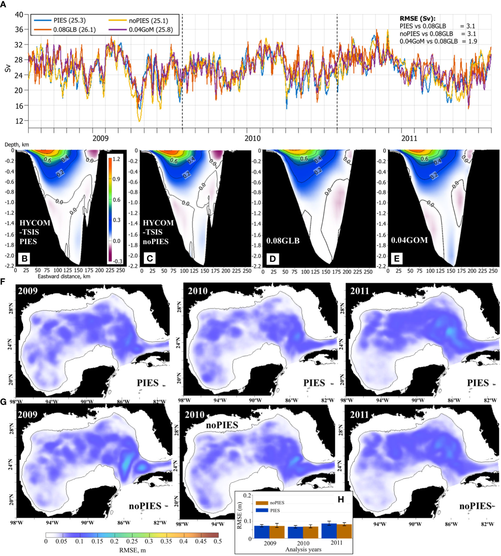
Figure 4 (A–E) Flow characteristics in Yucatan Channel from the 1/32.5° IAS HYCOM-TSIS OSEs, 0.08° Global HYCOM+NCODA reanalysis (0.08GLB), and 0.04° Gulf of Mexico HYCOM+NCODA reanalysis (0.04GOM). (A) Yucatan daily volume transport estimates (Sv). The mean volume transports over 2009–2011 are listed in parenthesis in the legend. On the right, RMSE (Sv) of the daily Yucatan transport estimates relative to the 0.08GLB is given. Vertical section of the mean along-channel velocity component (m s^-1, positive northward) in the Yucatan Channel from: (B) the 1/32.5° IAS HYCOM-TSIS OSE with PIES T/S profiles assimilated in the hindcast; (C) 1/32.5° IAS HYCOM-TSIS OSE without PIES T/S profiles; (D) 0.08GLB reanalysis; (E) 0.04GOM reanalysis. In (B–E), the horizontal axis is the eastward distance (km) along the section (the Yucatan Shelf is on the left), the vertical axis is depth (km). (F) Annual RMSE between SSH (m) from the OSE analysis runs with assimilated PIES T/S profiles and from the 0.04GOM reanalysis for April 2009 – November 2011 (time interval of the PIES observations). (G) Same as (F) but OSE with no PIES T/S profiles. (H) Median and IQR of the RMSE from “PIES” and “noPIES” OSEs by years.

The characteristics of the Yucatan Channel flow derived from the OSE analysis and the reanalysis fields are in good agreement (Figure 4A). The flow structure captures major features of the flow (Figures 4B–E) reported from observations (e.g., Sheinbaum et al., 2002; Abascal et al., 2003). The strong Yucatan current flows northward with the core located in the upper western part of the channel with speeds exceeding 1 m s^-1. Along the eastern side, there is a strong surface Cuban Countercurrent. Interestingly, the Cuban countercurrent in the HYCOM-TSIS OSEs (Figures 4B, C) is stronger (about 0.2 m s^-1) than in both reanalyses (about 0.1 m s^-1, Figures 4D, E). Reported mean speeds in the Cuban Countercurrent exceed 0.2 m s^-1 (Abascal et al., 2003), but it has a large interannual variability (Sheinbaum et al., 2002). Deep undercurrents in the western and eastern sides of the channel are also present in the simulations. The Yucatan Undercurrent – the outflow that follows the Yucatan slope between 800 m and the bottom – is only weakly pronounced in the 0.08GLB reanalysis (Figure 4D), but is notable in the OSEs and 0.04GOM reanalysis.

The root mean square error (RMSE) is computed between the SSH fields derived from the OSEs (“PIES” and “noPIES”) and from the 0.04GOM reanalysis (Figures 4F, G). From a visual inspection, the impact of the assimilated T/S profiles derived from PIES observations on the SSH is more notable in 2009 and 2010, and less in 2011. For both OSEs, the RMSE has comparable values and spatial distribution over the GoM. During all years, the RMSE of the OSEs is low (<0.1 m) over the most of the domain, but increases (up to 0.2 m) in the eastern GoM over the LC region. In this region, the OSEs exhibit some differences. In 2009 and 2010, the “noPIES” OSE has elevated RMSE in the middle of the LC region (between 22°N and 26°N) that is smaller in the “PIES” OSE. This is the region where LC “necking” occurs before the LC sheds an eddy, the so-called “necking-down” separation (Vukovich and Maul, 1985; Zavala-Hidalgo et al., 2003). Presumably, assimilating PIES observations improves the LC behavior in this region, although the PIES sites are located farther north (Figure 1). In 2011, the “noPIES” OSE has slightly lower RMSE in the LC region compared to the “PIES” OSE. Spatial RMSE of the SSH in the OSE analysis runs is comparable for all years (Figure 4H).

3.2 OSE forecasts

Added value of the PIES T/S profiles to the predictability of the LC system is investigated in 3-month forecast simulations initialized from the “PIES” and “noPIES” OSE hindcasts. The first 3-month forecast starts on May 1, 2009. The other 3-month forecasts are performed at a one-month interval until December 1, 2010, providing twenty 3-month forecasts for each OSE (“PIES” and “noPIES”). The predictive skill of the forecasts is then evaluated based on the RMSE of the daily SSH and the MHD of the LC and LCE contours derived from the forecast daily SSH fields. The forecasts are compared against the 0.04GOM reanalysis.

In both forecast groups, the RMSE increases with time as the forecasts’ accuracy degrades (Figure 5). The most prominent increase of the RMSE is in the LC region and the error is larger in the forecasts initialized from “noPIES” OSE. The growth rate of the mean RMSE is faster during the first several weeks and then slows down as the error approaches the saturation value (Figure 6A), in agreement with the forecast error theory (Lorenz, 1965; Dalcher and Kalnay, 1987). There is a wide spread in the RMSE estimates across the individual forecasts because of the spread in the initial error. Larger errors grow faster resulting in the lower predictive skills and shorter predictability of the forecasts.

FIGURE 5

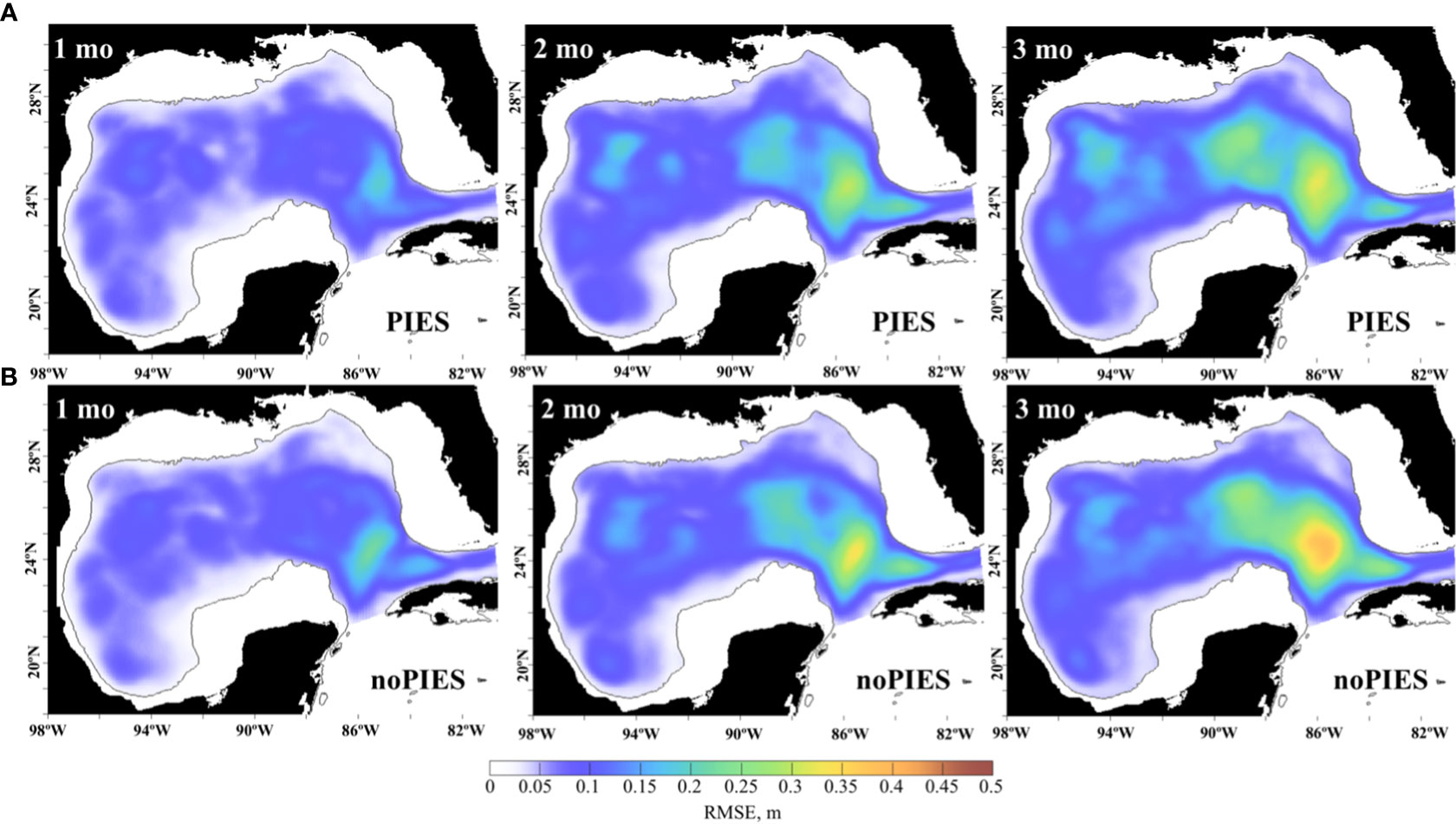
Figure 5 Monthly mean RMSE between daily SSH (m) from the OSE 3-month forecasts in 2009–2010 and from the 0.04GOM reanalysis. The forecasts initialized from the OSE with PIES T/S profiles (top row, A) and the OSE with no PIES T/S profiles (bottom row, B). The RMSE is averaged by the forecast months (in columns), so that the monthly statistics are derived from roughly 30 days of 20 forecasts.

FIGURE 6

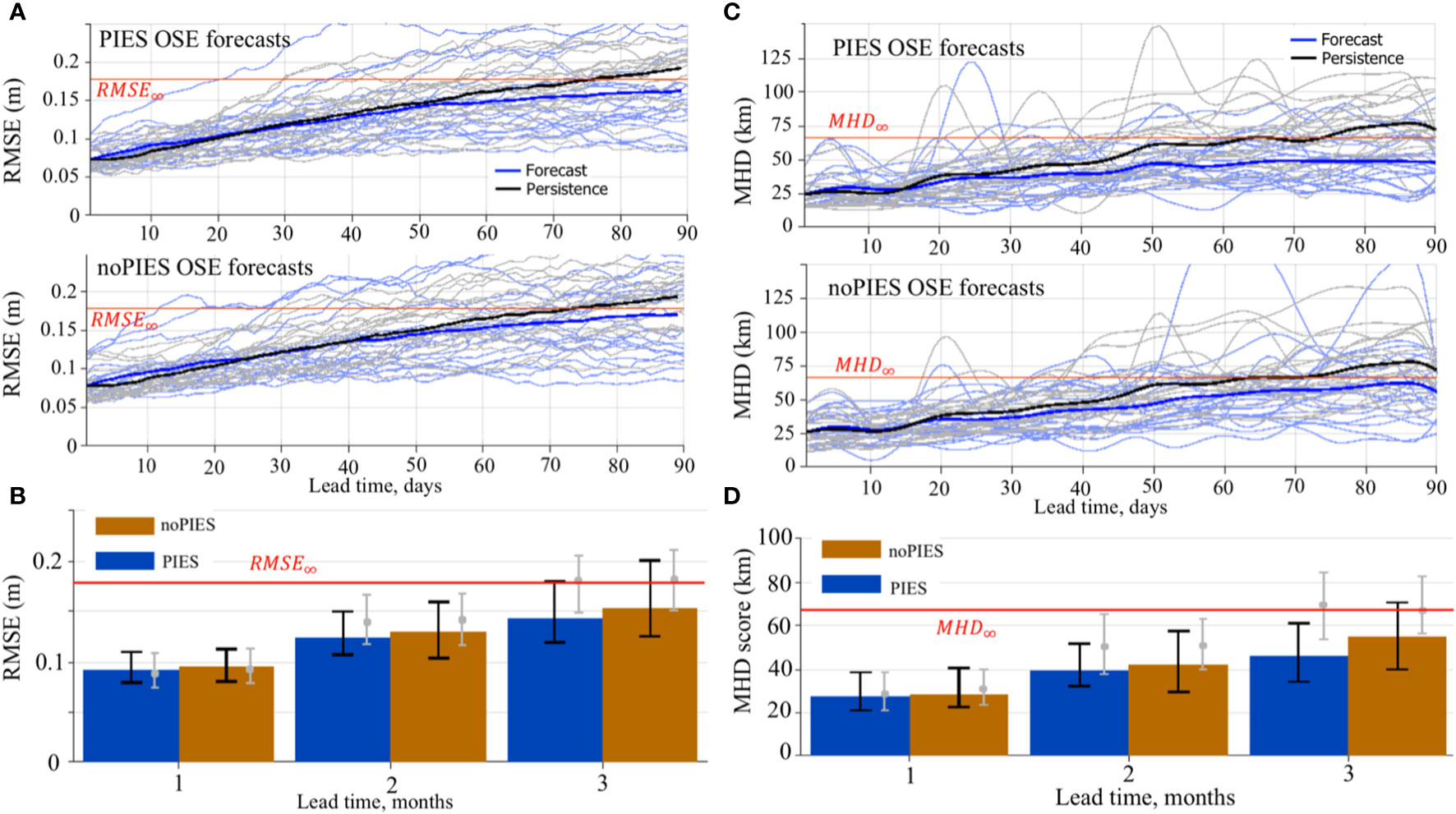
Figure 6 (A, B) RMSE (m) between SSH from the forecasts initialized from the “PIES” and “noPIES” OSE analysis runs and SSH from the 0.04GOM reanalysis. (A) RMSE of the individual 3-month forecasts (light blue) and corresponding persistency prediction (grey lines). The bold blue line is the mean RMSE over all individual forecasts. The black is the mean RMSE of persistency forecasts. The horizontal red line indicates RMSE_∞ (95% of the saturation value). (B) The median (the colored bars) and the IQR (the black vertical lines) of the RMSE. The RMSE are grouped by the forecast months. The grey bullet and the vertical lines indicate the median and the IQR of the RMSE between the persistence and the 0.04GOM reanalysis. (C, D) MHD scores (km) of the OSE forecasts. The MHD is computed for the LC/LCE fronts derived from the SSH fields of the OSE forecasts and the 0.04GOM reanalysis. (C) MHD scores of the individual 3-month forecasts (light blue) and corresponding persistency prediction (grey lines). The bold blue line is the mean MHD over all individual forecasts. The black is the mean MHD of persistency forecasts. The horizontal red line indicates MHD_∞. (D) Median (bars) and the IQR (the black vertical lines) of the MHD scores of the OSE forecasts grouped by the forecast months. The grey bullet and the vertical lines indicate the median and the IQR of the MHD of the persistence.

The monthly mean RMSE in Figures 5, 6B shows that the forecasts initialized from the OSE assimilating PIES T/S profiles perform slightly better than the “noPIES” forecasts. The median (and the mean) RMSE is less than $RMS{E}_{\infty }$ indicating that most forecasts from both groups have not lost predictability by the end of the 3^rd month of the forecast cycle. A higher percentage of the “PIES” forecasts retain predictability by the end of the forecast cycle (almost 75% “PIES” vs ~63% “noPIES”) suggesting added value of subsurface T/S profiles from PIES assimilated in the OSE analysis. Compared to the persistence RMSE, the forecasts from both groups have similar ratio to persistence skills in the 1^st month. In the 2^nd and 3^rd months, the RMSE of the forecasts is lower than persistence. Our OSE forecasts demonstrate longer predictability when compared to the results of Zeng et al. (2015) where the number of forecasts that failed to pass the threshold value for skillful prediction quickly increased after 4 weeks. In the OSE forecasts, >75% of “noPIES” forecasts possess predictive skills by the end of the 2^nd month of the forecast window.

Similar to RMSE, the MHD scores increase with lead time due to degrading accuracy of the forecasts in predicting the LC front (Figure 6C). The growth rate of mean MHD is slower for “PIES” forecasts than for “noPIES” but in both cases, the mean does not exceed $MH{D}_{\infty }$ during the 3-month forecast time. Statistics (the median and the IQR) of the MHD scores indicate similar skills in predicting the LC front for both “PIES” and “noPIES” forecasts groups during the 1^st month (Figure 6D). The difference between the MHD scores for two forecast groups increases in the 2^nd and 3^rd months with “PIES” forecasts on average demonstrating better skills. In contrast to the RMSE, more forecasts from both groups (>75% “PIES” and ~70% “noPIES”) still possess predictability by the end of the 3^rd month. Both forecasts groups barely outperform persistence in predicting the LC front during the 1^st month, but have markedly better skills in the following months.

4 Observing system simulation experiments

In the second series of the experiments (OSSEs), the IAS HYCOM solution is relaxed to the GLORYS12 reanalysis outside of the GoM NEMO NR domain to provide a similar ocean state to that of NEMO along the NEMO domain. In the OSSE hindcasts, the assimilated fields are subsampled from the NR (section 2.2) in a similar fashion to that of the observations (existing or projected), i.e. at the same locations and with the same temporal and spatial frequencies. In this series of experiments, the OSSEs are carried out to assess added value of different types of observations, their location and spatial coverage to the predictability skills of the forecasting systems. During the OSSEs, the nature run solutions are sampled at the space-time locations of satellite SST measurements, along-track SSH, and PIES T/S profiles to form daily synthetic observations for assimilation into the numerical solutions. These OSSEs address the following objectives: (1) assess the sensitivity of the forecasts to the various types of observations currently available; (2) evaluate added value to the forecasts from proposed new types of observations or expansion of observing sites in the eastern GOM; and (3) evaluate predictability of the LC system for idealized cases when the information about the true state is unlimited resulting in smaller error between the true state and analysis. Two time periods representing active and stable LC states are selected from the NR for the OSSE data assimilative hindcasts. During the first time period, June–September 2011, the shape of the LC changes considerably during several detachments and reattachments of the LCEs. By contrast, the LC exhibits small variability with one LCE reattachment during the second time period, January–May 2012. Note that the model states during these time periods do not necessarily represent the true ocean states because the NR is free-running and not data assimilative.

4.1 Design of the OSSE hindcasts

To address the objectives of the OSSEs, nine hindcasts were performed with different set of NR fields assimilated into the 1/32.5° IAS HYCOM-TSIS (Figure 7). The OSSEs can be combined into 3 main groups, following the objectives. The first group of hindcasts (Figures 7A–D) assimilate types of observations commonly used in the operational GoM forecasts as well as the PIES observations that are currently being evaluated for delivering data in near-real-time. Hindcast “AVISO-PIES-SST” represents the case with the most complete set of synthetic observations including 4–day composite SLA from AVISO swath data, T/S profiles from PIES, and SST from GHRSST gridded fields (Figure 7D). Hindcasts “AVISO-PIES”, “AVISO”, and “AVISO-1” assimilate reduced information: withheld SST (Figure 7C), no T/S profiles and no SST (Figure 7B), SLA from only 1 satellite (Figure 7A).

FIGURE 7

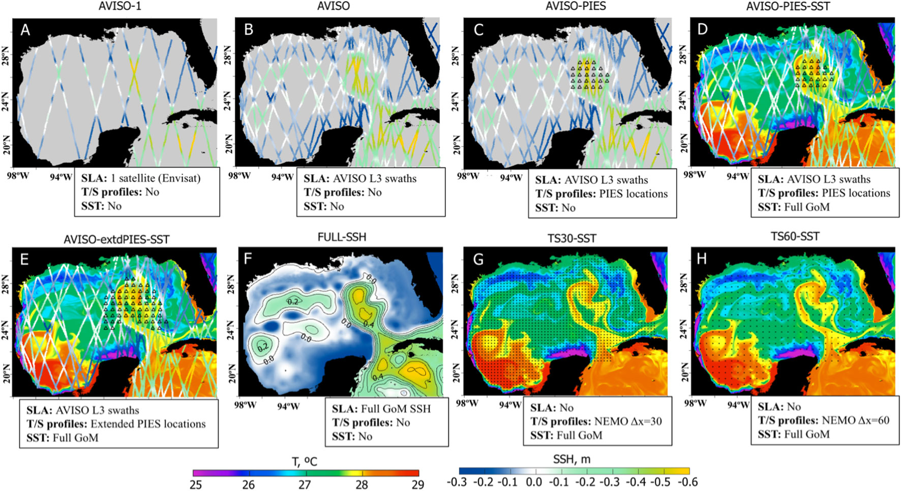
Figure 7 Design of the OSSEs. The maps show data fields assimilated into the OSSE hindcasts. Assimilated fields are listed below the maps. (A) SLA from one (Envisat) satellite (4 days composite). The colored lines show NEMO SSH (Nature Run) on June 1, 2011 interpolated into satellite swaths. (B) Same as (A) but all available satellites on the analysis day (4 days composite). (C) Same as (B) additionally with T/S profiles derived from PIES observations. (D) Same as (C) additionally with SST. This experiment replicates the most complete set of observations presently available for assimilated runs. The colored field in the background shows SST from the NEMO NR (June 1, 2011). (E) Same as (D) but with T/S profiles from extended PIES. (F) Full SSH field from the NEMO NR (June 1, 2011). (G) T/S profiles at every 30th NEMO grid point and SST. (H) T/S profiles at every 60th NEMO grid point and SST.

The second group of OSSE hindcasts evaluates the added value of assimilating additional T/S profiles provided by expanded PIES arrays in the LC region (hindcast “AVISO-extdPIES-SST, Figure 7E). The expansion of the PIES and mooring sites in the eastern GOM for better observation of the LC and LCE was proposed at the time of UGOS-1. This experiment is similar to hindcast “AVISO-PIES-SST” (Figure 7D), except for the additional PIES T/S profiles that are assimilated during the hindcast.

The last group combines idealized cases when unlimited information is available for constraining the 1/32.5° IAS HYCOM simulation. In hindcast “FULL-SSH”, complete information about the sea surface height (SLA from the NR) is provided to the data assimilation algorithm (Figure 7F). In the two other hindcasts (“TS30-SST” and “TS60-SST”), only subsurface T/S fields and SST are assimilated and no SLA fields are used. For these hindcasts, the T/S profiles are derived from the NR at every 30^th (Figure 7G) and 60^th (Figure 7H) NEMO grid points in the GoM. Thus, the two hindcasts differ in the density of T/S profiles over the GoM.

The last hindcast (“NEMO-INT”) represents a highly idealized case imitating a perfect assimilation of the 3D ocean state into the forecasting system. There are two sources of errors contributing to forecast error: errors in the initial conditions and errors associated with numerical models used in the forward simulation. In complex forecast systems, these two components cannot be easily separated. One practical way for doing this is to provide perfect initial conditions and evaluate the forecast error growth. In order to substantially reduce the uncertainty in the predictive skills of the model due to errors in the data assimilation process, the NEMO fields are directly interpolated into the 1/32.5° IAS HYCOM horizontal grid and vertical layers. Outside the NEMO domain (Figure 1), the GLORYS12 fields are interpolated onto the IAS HYCOM grid. This approach significantly reduces the error of the “analysis” (demonstrated in the following section) providing the best possible initial state for the OSSE forecast experiments. Therefore, this experiment provides an estimate of the best predictive skill for this configuration of the 1/32.5° IAS HYCOM if a perfect initial state could be provided by the analysis. Validation of the SSH, subsurface T/S fields, and the LC frontal position have shown a very close match of the interpolated fields to the NR. Hindcast “NEMO-INT” is not a true analysis run and it is therefore not discussed in the OSSE hindcasts section 4.2. The forecasts initialized from the interpolated NEMO fields are analyzed and compared to the other OSSE forecasts.

4.2 Analysis of the OSSE hindcasts

4.2.1 RMSE analysis

The RMSE is calculated from the daily SSH fields derived from the HYCOM analysis and NR and averaged over 2011–2012 (Figure 8A). The RMSE maps show conspicuous differences in the OSSEs depending on the amount of information assimilated in the analysis. As expected, the hindcast with the lowest quantity of information (“AVISO-1” using experiments’ notations in Figure 7) demonstrates the poorest performance with high RMSE over the GoM compared to other OSSEs. Whereas, the “TS30-SST” forecast with the most complete set of T/S profiles has the best performance with the overall lowest RMSE. The hindcast “TS60-SST” that assimilates T/S profiles with the coarser spatial coverage (half of “TS30-SST”) has comparable RMSE scores, but the error is elevated along the eastern side of the LC.

FIGURE 8

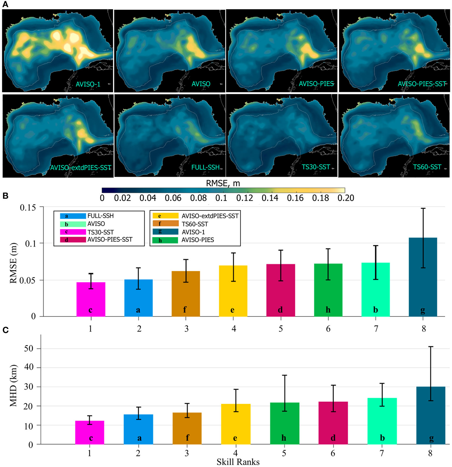
Figure 8 (A) Maps of mean RMSE (m) between daily SSH fields from the OSSE analysis runs shown in Figure 7 and from the NR (NEMO). The RMSE is averaged over 2011–2012. The gray contour is the 200-m isobath. The OSSEs are indicated in the maps. (B) RMSE (m) between SSH from the OSSE analysis runs and the NR over the hindcast period (2011–2012). The colored bars show the median RMSE with colors corresponding to the OSSEs. The hindcasts are ranked based on the median RMSE. The vertical black lines indicate the IQR. The letters in the bars are for ease of color identification. (C) MHD scores computed for the LC/LCE contours derived from the OSSE analysis SSH fields versus the NEMO NR. The bars show the median MHD scores by OSSEs. The hindcasts are ranked based on the median MHD score.

Predictive skills of the OSSE hindcasts are compared in terms of the median values of the time-averaged SSH RMSE fields (Figure 8B). The OSSE ranking matches the expectation. The hindcast constrained by the most complete 3D hydrographic fields (“TS30-SST”) has the best performance followed by the hindcast that assimilates 2D SSH provided at every model grid in the GoM (“FULL-SSH”). Then the hindcast performance degrades as the amount of the assimilated information decreases. The hindcast with only 1 AVISO track used as a constraint (“AVISO-1”) has the poorest performance with distinctly higher RMSE. The hindcasts ranked from 4 to 7 have very small difference in the RMSE scores. All these hindcasts have assimilated AVISO SLA, but differ in the assimilation of SST and PIES T/S profiles. The hindcast that assimilates T/S profiles from the extended PIES array has a better skill than that the experiment assimilating data from the actual PIES array, but the difference is too small to be significant.

4.2.2 MHD of the LC and LCE frontal positions

The MHD is computed for the LC and LCE fronts derived from demeaned daily SSH fields to quantify the similarity between the LC fronts in the OSSE analysis runs versus the NR. Examples of the LC and LCE fronts from the NR are shown in Figure 2 (top panels). The OSSE analysis runs are ranked based on the median MHD values (Figure 8C). There is a good agreement between rankings based on the MHD scores and RMSE, respectively. Again, the best performance has the simulations constrained by synthetic T/S profiles at every 30^th grid point (“TS30-SST”) followed by the “FULL-SSH” and “TS60-SST” hindcasts. The hindcast that assimilates limited SSH information (“AVISO-1”) has the lowest predictive skills. Adding subsurface T/S profiles to the satellite altimetry improves the accuracy of the LC front prediction in the hindcasts. The only difference between the MHD and the RMSE rankings is that “AVISO-PIES” swaps places with “AVISO-PIES-SST”; however, in both metrics the scores of these hindcasts are almost identical making the ranking of these two experiments uncertain.

4.2.3 Comparison of subsurface frontal positions

Anticyclonic eddies have a distinct signature in the subsurface hydrographic fields. The LC and LCEs in the GoM are associated with positive temperature anomalies that are tracked down to several hundred meters. Isotherms contouring warm water masses in the subsurface layers effectively delineate LC and LCEs and have been previously used for the LC/LCE identification and model skill assessment (Oey et al., 2005). Here, temperature anomalies at 200 m derived from the OSSEs are compared in order to assess the impact of different fields assimilated in the analysis on subsurface hydrographic fields. Temperature anomalies (ΔT) are computed from the 200 m temperature fields by subtracting the spatial mean. Then, ΔT = 2.5°C is used to contour the LC and LCEs (Figure 9A). Next, the MHD metric is employed to compare the OSSE 2.5°C contours against the NR for 2011–2012 (Figure 9B). The hindcasts are ranked based on the median of the MHD score. The best and the worst skills are found in the “TS30-SST” and “AVISO-1” hindcasts, respectively, similar to the ranking derived from the SSH contours (Figure 8C). The main difference in the MHD-based ranking between the surface and subsurface frontal positions is a decreased ranking of the “FULL-SSH” hindcast, with the ranking changed from the 2nd best to the 6th. All OSSE analysis runs that assimilate subsurface T/S profiles outperform the hindcasts constrained by the surface fields (“FULL-SSH”, “AVISO”, and “AVISO-1”). The ranking of the “FULL-SSH” analysis is lower (although insignificantly) than both hindcasts assimilating PIES and extended PIES T/S profiles. Note substantially better skill (lower MHD score) of the “AVISO-extdPIES-SST” OSSE compared to “AVISO-PIES-SST” demonstrating added value of the extended PIES array.

FIGURE 9

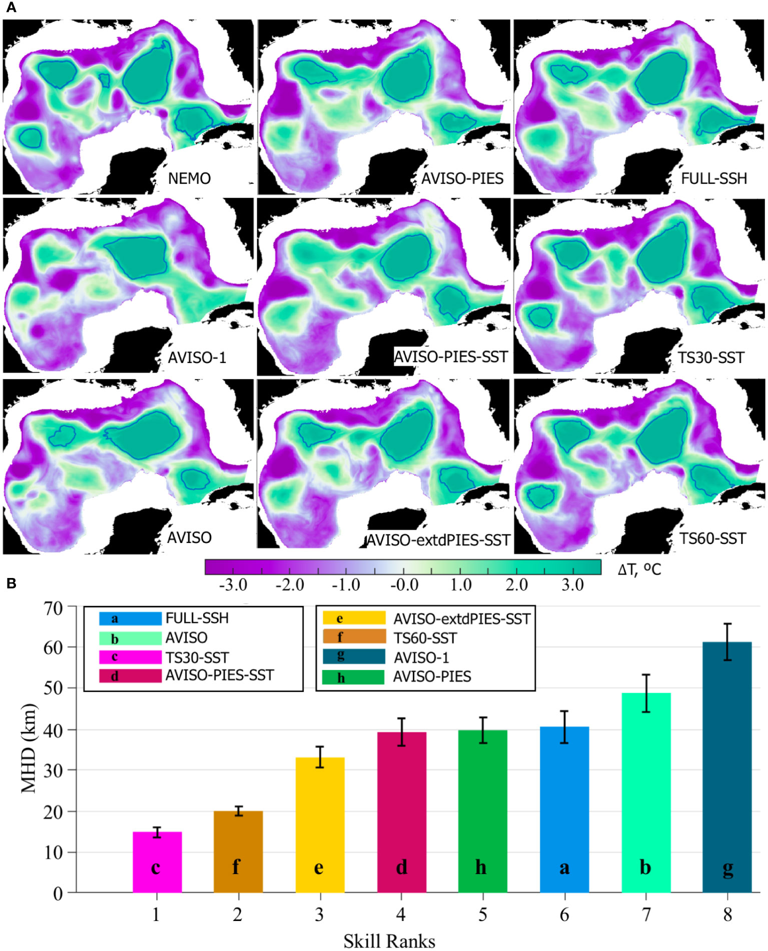
Figure 9 (A) Temperature anomaly (ΔT) at -200 m on July 9, 2011 from the NEMO NR and OSSE analysis. The contours delineate ΔT=2.5 °C isoline that tracks anticyclones and the LC. (B) MHD scores computed for the 2.5 °C contours of ΔT at -200 m (2011-2012) derived from the OSSE analysis fields and the NEMO NR. The colored bars are the medians with colors corresponding to the OSSE hindcasts. The hindcasts have been ranked based on the median MHD. The vertical black lines on top of the bars indicate the IQR.

4.3 Design of the OSSE forecasts

Two time intervals are selected for the OSSE forecast experiments. The first interval, the NR June-September 2011 time period, corresponds to an active or unstable phase of the LC characterized by extended position of the LC with potential LCE detachment (Figures 10A, B, E) or reattachment (Figures 10C, D). During this time period, the LC shape frequently changes due to several detachments and reattachments of LCEs (Figures 10A–E). The second time interval corresponds to the NR January–May 2012 (Figures 10F–J). At the beginning, the LC is in a stable position being retracted towards the Yucatan Channel in January (Figure 10F). During February – early March of 2012, the LC extends farther north (Figures 10G, H) and sheds a LCE in early March. The eddy reattaches to the LC about a week later (Figure 10I). Note that the shape and positioning of the LC in May 2012 is somewhat similar to that in January and February; this would make persistency with initial state from January or February a good forecast of the LC state in May as discussed in section 4.4.

FIGURE 10

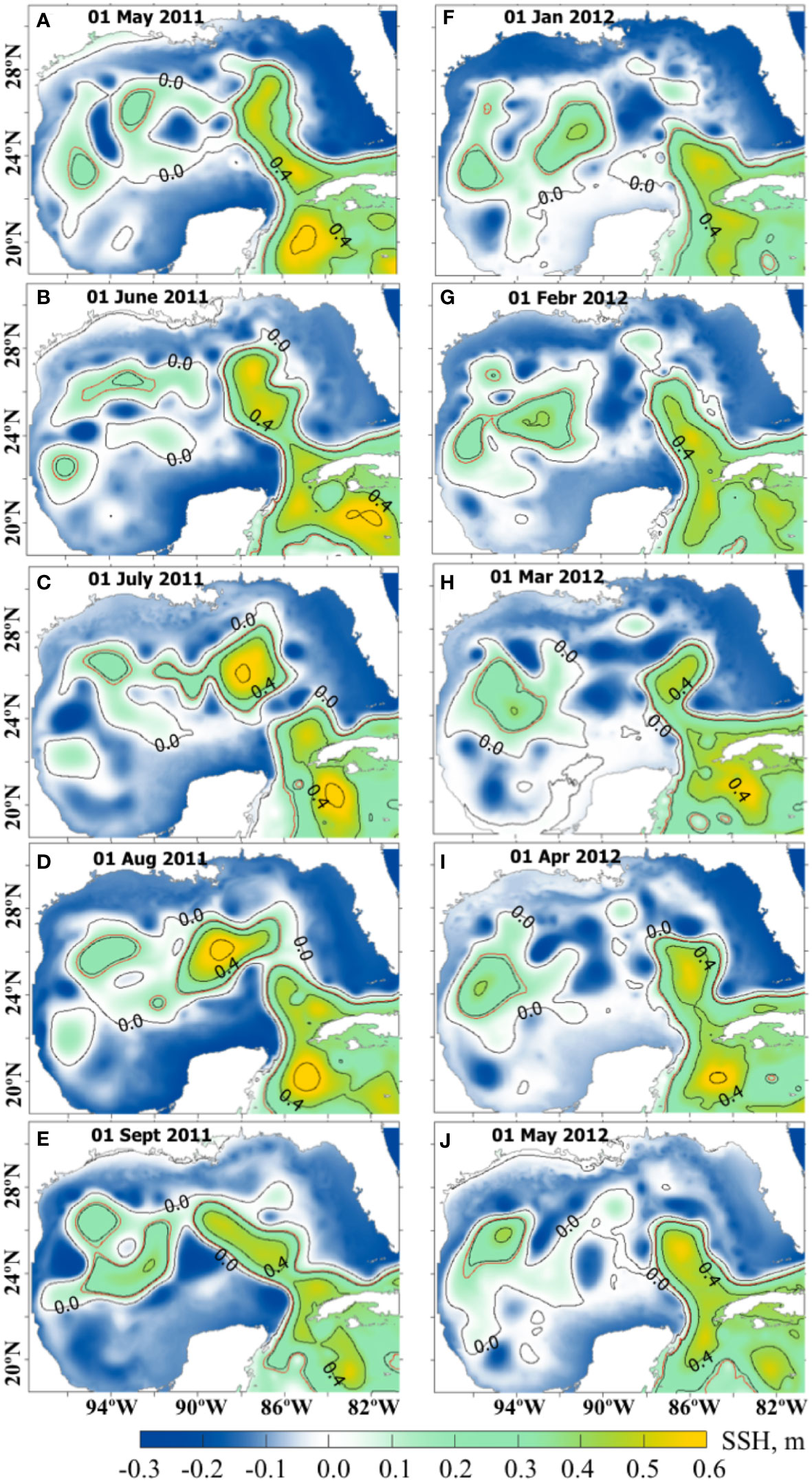
Figure 10 Daily SSH fields (m) from the NEMO NR. The left column (A–E) are SSH fields from May (A) – September (E) 2011 corresponding to the active state of the LC with several detachments and reattachments of the LCE. The right column (F–J) are SSH fields from the time interval January (F) –May (J) 2012 during which the LC is in a more stable position. Contours are every 0.2 m starting from 0. The red line is the 0.17 m contour used as a definition of the LC and LCE fronts.

In the following set of numerical experiments, the three-month forecasts are initialized from the following OSSE analysis runs: “FULL-SSH”, “AVISO”, “AVISO-PIES-SST”, “AVISO-extdPIES-SST”, “TS30-SST” (Figure 7), and “NEMO-INT”. For each of these OSSE analysis runs, seven forecasts are initialized one week apart starting from May 1, 2011 until June 15, 2011 and seven forecasts initialized from January 1, 2012 until February 15, 2012. Therefore, there are 12 sets of forecasts (six OSSE group runs during two time intervals) that include seven individual forecasts initialized with a one-week interval and run forward for 3 months.

4.4 Analysis of the OSSE forecasts

4.4.1 RMSE analysis

The RMSE of the SSH is calculated using daily fields from the OSSE forecasts and from the NEMO NR. All forecasts within the same forecast group have been pooled together to provide monthly average RMSE for months 1 through 3 during 2011 (Figure 11) and 2012 (Figure 12). In all forecasts, the RMSE increases with time with the errors growing fastest in the LC area. In general, the predictability of the forecasts follows expectations dictated by the rankings of the OSSE analysis runs (Figures 8B, C). Forecasts initialized from the state with the smaller error have lower RMSE during the first 2 months and, in some cases, during the 3^rd month. For example, the performance of the “NEMO-INT” forecasts during the first 2 months is markedly better than all other forecasts, as expected due to the smallest error in the “NEMO-INT” analysis fields providing initial conditions for these forecasts. An interesting aspect of the 2011 RMSE maps is notably smaller errors over the LC region in the “AVISO-extdPIES-SST” during all 3 months of the forecast. The magnitudes and the pattern of the RMSE in these forecasts are similar to that from the “TS30-SST” forecasts that are initialized from the analysis more heavily constrained by the T/S profiles form the NR. Note that the error magnitude over the LC area is smaller in the “AVISO-extdPIES-SST” forecasts than that in the “AVISO-PIES-SST”.

FIGURE 11

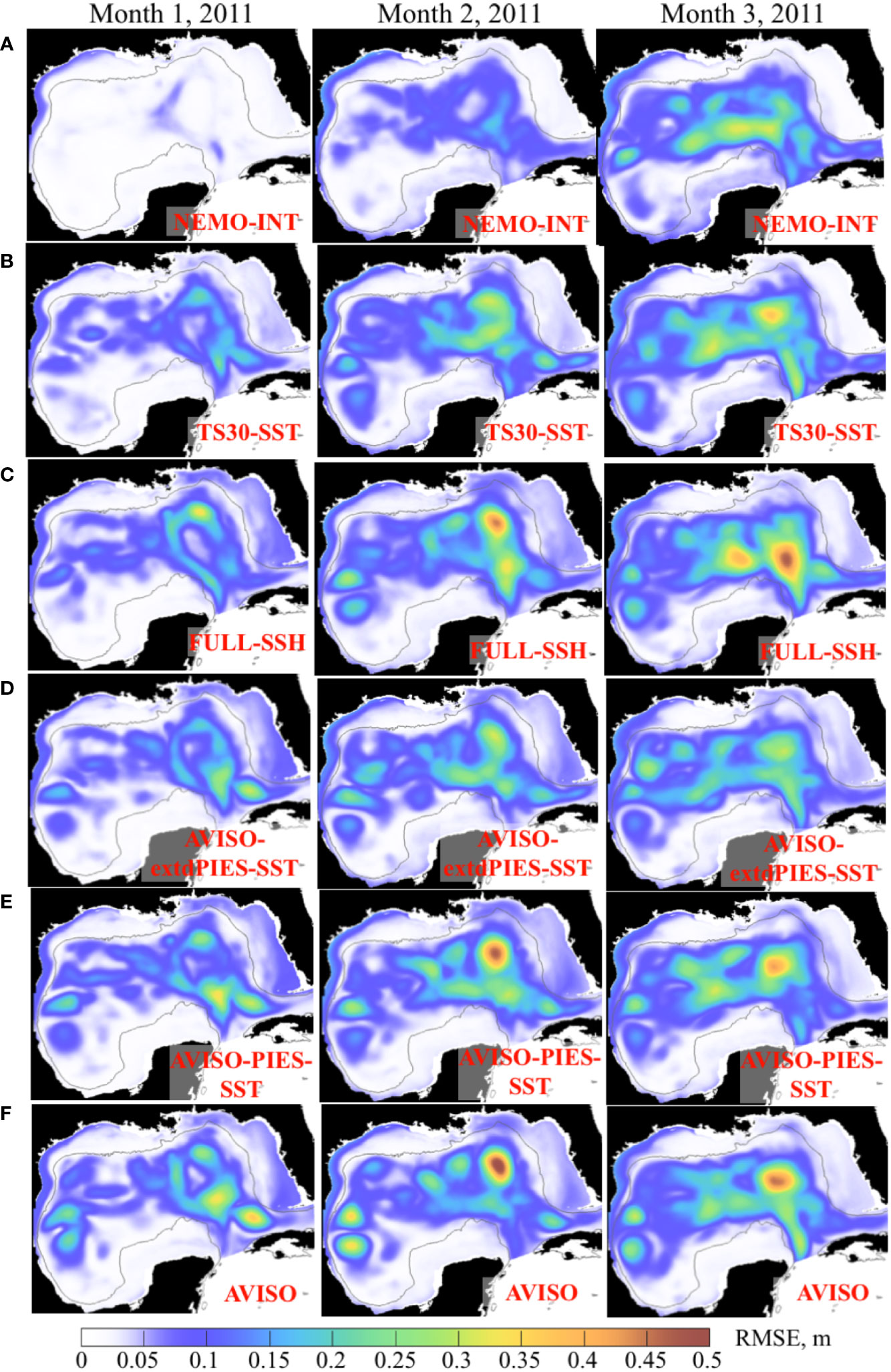
Figure 11 Monthly mean RMSE between SSH (m) from the 3-month OSSE forecasts started in May – June 2011 and the NEMO NR. The RMSE for months 1 through 3 are in the columns. The OSSE forecast groups are shown in the rows (A–F) with the forecast names shown in the maps.

FIGURE 12

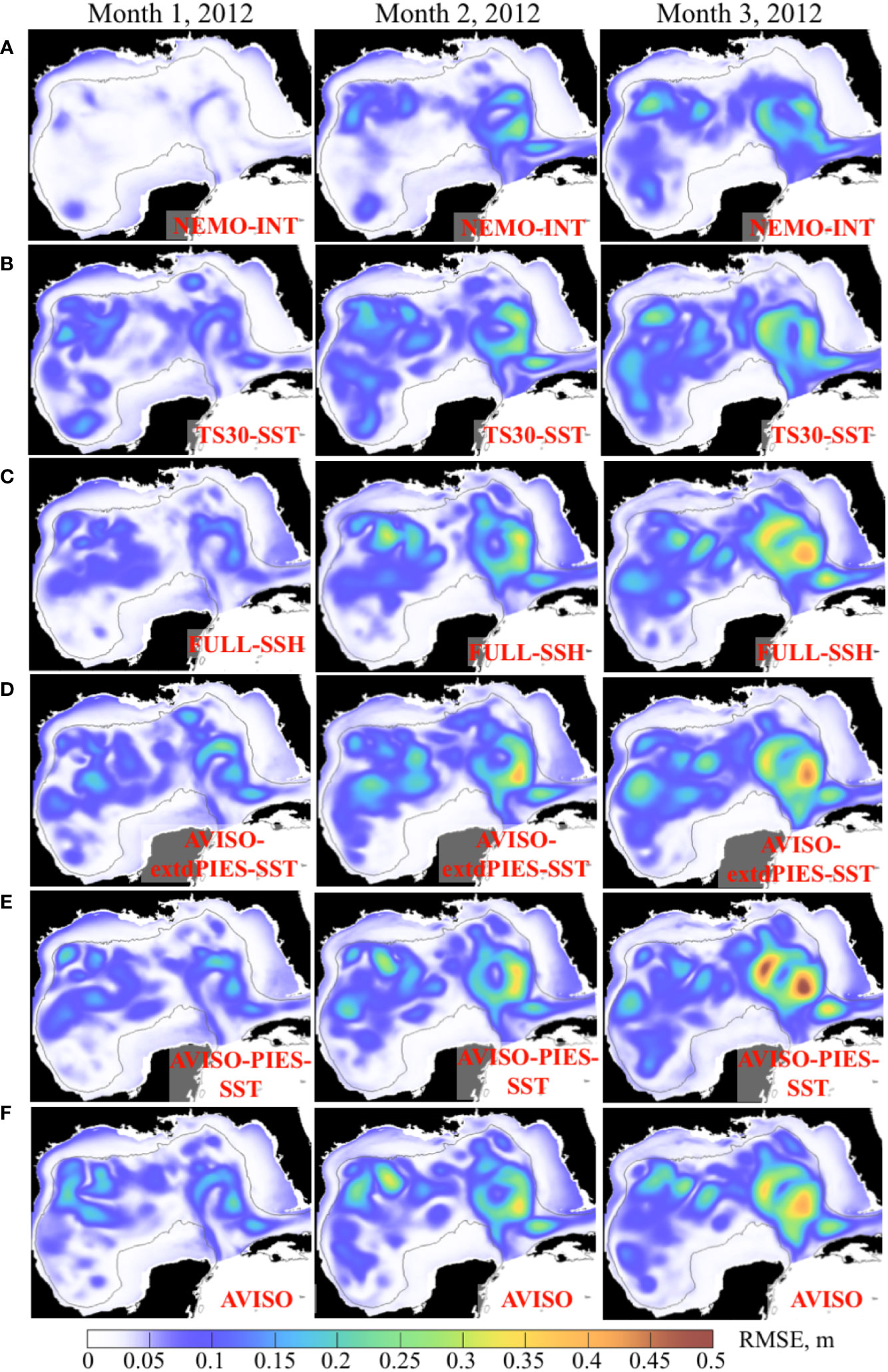
Figure 12 Monthly mean RMSE between SSH (m) from the 3-month OSSE forecasts started in January – February 2012 and the NEMO NR. The RMSE for months 1 through 3 are in the columns. The OSSE forecast groups are shown in the rows (A–F) with the forecast names shown in the maps.

The error growth rate in the forecasts is faster at the beginning of the forecast, then slows down as the error approaches the saturation value (Figure 13A) again in agreement with the forecast error theory (Lorenz, 1965; Dalcher and Kalnay, 1987). The “NEMO-INT” case is different in that the error growth rate is nearly linear during the 3-month time period. This stems from the fact that the initial errors in the “NEMO-INT” are very small (<0.01 compared to 0.05–0.08 in the other forecasts), and the time evolution of the small error is governed by linearized equations (Lorenz, 1965). Therefore, a linear growth rate is expected for small errors as nicely demonstrated by the “NEMO-INT” forecasts.

FIGURE 13

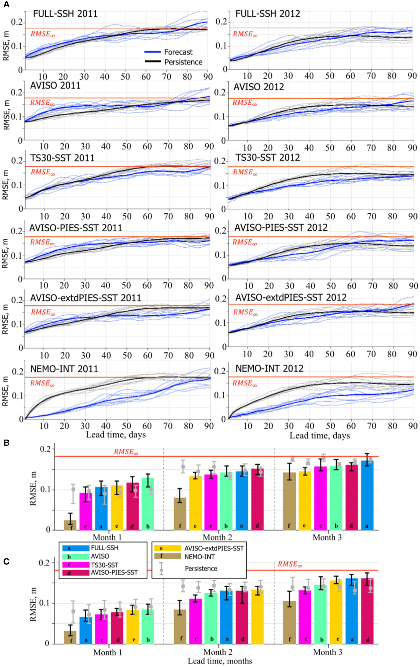
Figure 13 RMSE between SSH from the OSSE forecasts and the NR. (A) Daily RMSE for individual forecasts and persistence from the OSSE forecast groups during 2011 (left column) and 2012 (right column). The bold solid lines are the mean RMSE estimates for the forecasts (blue) and persistence (black). The horizontal red line indicates 95% of the saturation value (RMSE_∞ = 0.178 m). The bar diagrams (B, C) show median RMSE (m) of the forecasts by the OSSE forecast groups during months 1 through 3 started in May-June 2011 (B) and January-February 2012 (C). Within each month, the OSSE forecast groups are ordered according to the ranks based on the median RMSE. The vertical black lines on top of the bars indicate the IQR. The grey line and the bullet show the IQR and the median, respectively, of the persistence corresponding to the OSSE forecast group. The horizontal red line indicates RMSE_∞.

The performance of the OSSE forecasts is ranked based on the median of the spatially averaged daily RMSE (Figures 13B, C). For the forecasts started in May-June 2011, the ranking during the first month of the forecast matches the expectation assuming that the forecast with the smallest error in the initial state from the analysis provides a more accurate prediction. Therefore, the ranking of the OSSE forecasts would be expected to follow the ranking of the corresponding OSSE analysis runs (Figure 8B). This is true for the 1^st month. The forecasts “NEMO-INT”, initialized from the best initial conditions with the smallest assimilation error (interpolated fields), are ranked first demonstrating significantly smaller RMSE than the other forecasts. The RMSE in this forecast group decreases and is only slightly smaller than the RMSE of the second-best forecast by the end of the forecast period. The “TS30-SST” forecasts have the best second ranking followed by the “FULL-SSH”. The forecasts in these two groups were initialized from the OSSE analysis that assimilated the most complete synthetic observations compared to the other hindcasts. The “AVISO” forecasts have the lowest score, which is expected given substantially smaller amount of information constraining the solution in the OSSE analysis providing initial state to these forecasts. Therefore, the ranking for the first month demonstrates an expected relation between the accuracy of the initial condition and the quality of the forecast. However, this expected ranking breaks in the second and third months where the “AVISO” forecasts have moved two positions up and the “FULL-SSH” to the end. The order of the forecasts in months 2 and 3 is unexpected and does not agree with the OSSE analysis ranking in Figure 8B. This result shows that the error in the forecasts grows at a different rate, which is evident in Figure 13A.

In 2012, the “NEMO-INT” and “TS30-SST” forecasts also have persistently higher rankings as in 2011. Again, the “FULL-SSH” forecasts ranking unexpectedly decreases by the end of the forecast period, whereas “AVISO” forecasts are third best in the second and third months. Rankings of “AVISO-PIES-SST” and “AVISO-extdPIES-SST” are inconsistent. In 2012, the prediction skills of “AVISO-extdPIES-SST” forecasts are not as high as during 2011 when compared to the other forecasts, although the difference in RMSE among some of them is small.

Similar to the OSEs, the OSSEs (except for “NEMO-INT”) struggle to outperform persistence during the 1^st month in 2011. The only two forecast groups that outperform persistence in terms of the SSH RMSE during all forecast months in 2011 and 2012 runs are “NEMO-INT” and “TS30-SST”. In 2011, the skills of other forecasts are lower than persistence in the 1^st month, higher in the 3^rd month, and mixed in the 2^nd month. In 2012, all forecasts have better skills than persistence in 1^st and 2^nd months. During the 3^rd month, the forecasts are ranked lower than persistence except for “NEMO-INT” and “TS30-SST”. The persistence-based estimate of the forecast skills is somewhat inconsistent with the assessment of predictability of the forecasts. In all cases (except for “FULL-SSH” in month 3 of 2011), the median RMSE and the upper IQR are less than $RMS{E}_{\infty }$ indicating that the model predictive skills exceed 3 months in 75% forecasts.

4.4.2 MHD of the LC and LCE fronts

The forecast skills of the 1/32.5° IAS HYCOM in predicting the LC front are assessed employing the MHD that is computed for the LC and LCE fronts derived from daily SSH fields in the OSSE forecasts and the NR. An example of the LC/LCE contours derived from SSH fields of one of the OSSE forecasts and NR is shown in Figure 14. The MHD scores are computed between the LC/LCE contours from the forecasts and the NR (the MHD score is listed in blue), as well as between the forecast and the persistence (grey). Scores greater than $MH{D}_{\infty }$ (6.3 km) demonstrate a lack of skills in predicting the LC/LCE frontal position.

FIGURE 14

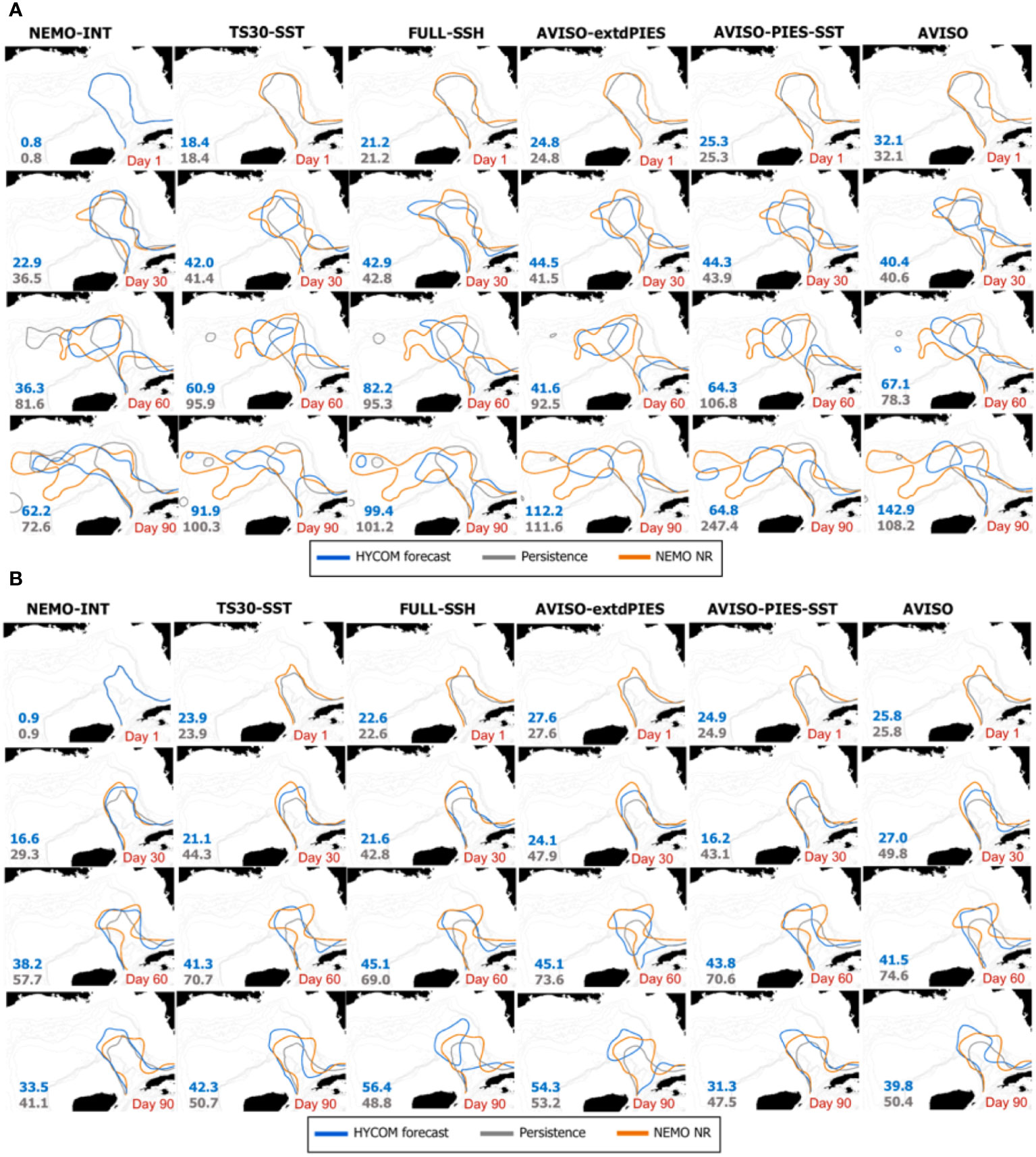
Figure 14 Example of the LC/LCE contours (fronts) from one of the OSSE forecasts in each forecast group (in columns) and corresponding contours from the NEMO NR during 2010 (A) and 2011 (B). The blue contours correspond to the OSSE forecasts and the orange contours are from the NR. The grey contours show persistence prediction. In the first row in (A, B), the initial state (day 1) is shown. The LC contours from the OSSE forecasts and persistence coincide demonstrating a perfect match of the initial contours from the “NEMO-INT” and the NR. The numbers are MHD scores for the shown contours from the forecast - NEMO NR (blue) and persistence - NEMO NR (orange).

Compared to the RMSE, the MHD scores of the OSSE forecasts exhibit more oscillating behaviour superimposed on the overall increasing trend (Figure 15A). The oscillations of the MHD scores are due to the rapid changes in the shape of the LC front during eddy detachment–reattachment events, the timing of which is not correctly predicted by the forecast. Nevertheless, the overall trend in the MHD scores meets the expectation and agrees with the RMSE results. The MHD time series demonstrate degrading forecast skills of predicting the LC frontal position with time. In 2011, the mean MHD of all forecast groups has exceeded or reached $MH{D}_{\infty }$ after ~60 days. By contrast, the mean MHD stays below $MH{D}_{\infty }$ through the end of the runs for the all forecast groups. The difference in the forecast performance is due to different LC phases (Figure 10). In 2011, the NR LC was active with several eddy detachment-reattachment events. Whereas in 2012, the NR LC was less active resulting in a more accurate forecasts of the LC front. Note the decreasing mean MHD for persistence during 2012 by the end of the 3-month period in contradiction to the expected increase. The decreasing MHD is a consequence of similar LC shapes at the beginning and end of the forecast time period (Figures 10F, J) by chance making persistence a good prediction of the LC front.

FIGURE 15

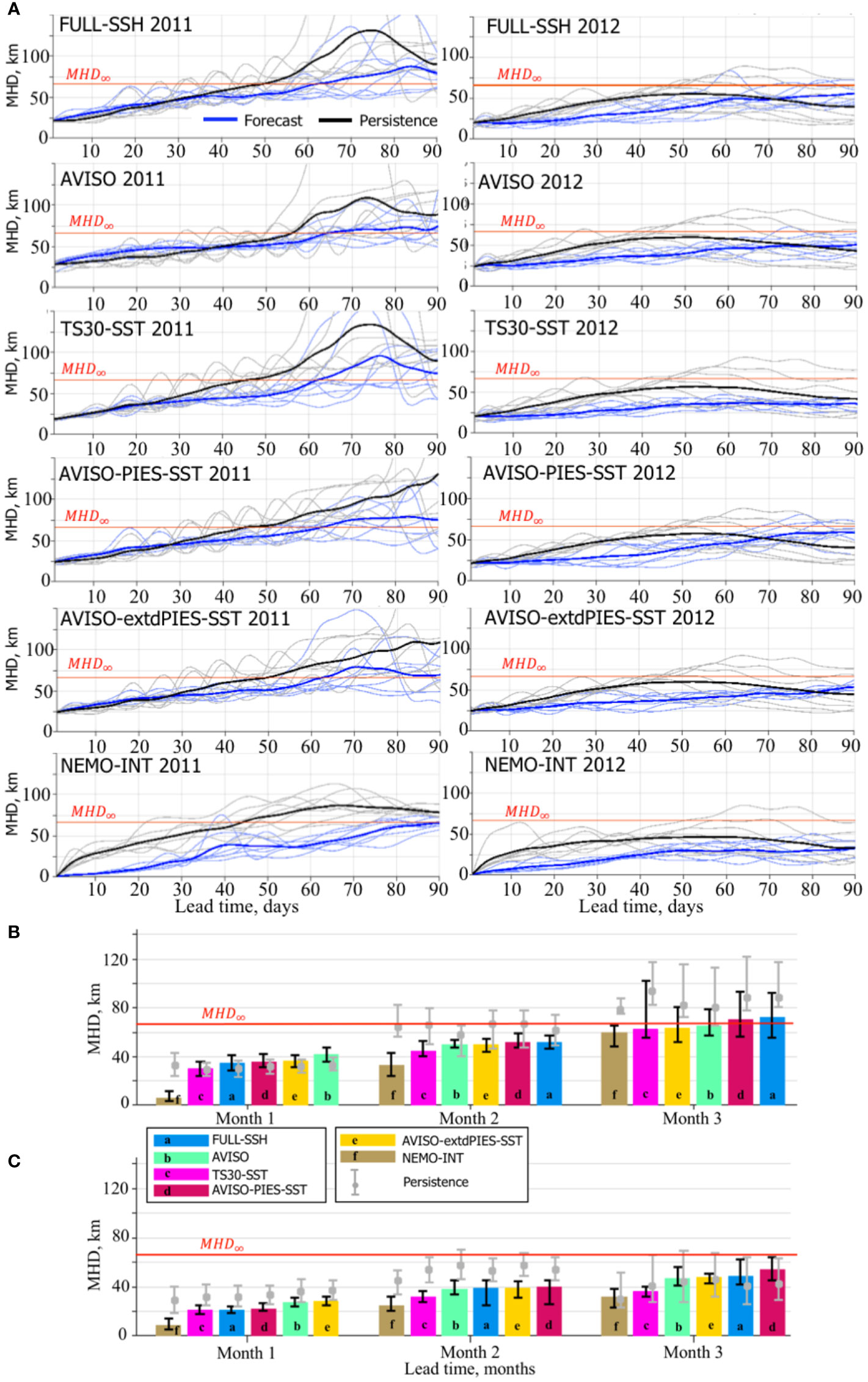
Figure 15 MHD scores for LC/LCE fronts derived from OSSE SSH forecasts and the NR. (A) Daily MHD scores for individual forecasts and persistence from the OSSE forecast groups during 2011 (left column) and 2012 (right column). The bold solid lines are the mean MHD scores for the forecasts (blue) and persistence (black). The horizontal red line indicates 95% of the saturation value (MHD_∞ = 66.3 m). The bar diagrams (B, C) show median MHD score (km) from forecasts within the forecast group (shown with colors and letters corresponding to the OSSE forecast groups) during forecast months 1 through 3 started in May-June 2011 (A) and January-February 2012 (B). Within each month, the OSSE forecast groups are ranked based on the median MHD score. The vertical black lines on top of the bars indicate the IQR. The grey line and the bullet on the line show the IQR and the median of the persistence corresponding to the OSSE forecasts. The horizontal red line indicates MHD_∞.

There is a good agreement in the rankings based on the RMSE (Figures 13B, C) and the MHD metrics (Figures 15B, C). “NEMO-INT” forecasts have the best predictive skills and are ranked first for all months in both forecast time periods (2011 and 2012). The “TS30-SST” forecasts are second best, in agreement with the expectation. Similar to the RMSE metric, the “FULL-SSH” forecasts quickly loose predictive skills moving to the last (2011) and second last (2012) rankings at the end of the forecast period. By contrast, the “AVISO” forecasts unexpectedly improve rankings in the 2^nd and 3^rd months. The “AVISO-extdPIES-SST” forecasts have better predictive skills than the “AVISO-PIES-SST” forecasts after the 1^st month.

The MHD scores indicate similar predictive skills of the OSSEs, although there is a bigger difference in the performance during the 3^rd months across OSSEs in 2011 and 2012. During a more active LC (year 2011), predictability of the forecasts is lost during the 3^rd month in >50% of cases except for the “NEMO-INT”. By contrast, >75% of the OSSE forecasts demonstrate high predictive skills of the LC by the end of the 3^rd month.

The “NEMO-INT” forecast group is the only one that outperforms persistence in 2011 and 2012, except for the 3^rd month in 2011 when the scores are similar. In 2011, other forecasts struggle to outperform persistence during the first month and substantially outperform the persistence in the 2^nd and 3^rd months. In 2012, the forecasts outperform the persistence for the first two months and underperform during the last month of the forecast window. In 2011, the initial state of the LC quickly evolves into an unstable state in the forecasts, whereas it remains nearly unchanged for several weeks in the NR, as demonstrated by the example in Figure 14A. At the beginning of the forecast, the LC front in the “NETMO-INT” perfectly matches the LC contour in the NR. In the other forecasts, there is a notable difference in the initial LC shapes compared to the NR. In 2011 after 30 days, the forecasts tend to predict LCE shedding (except for the “NEMO-INT” and “FULL-SSH”), whereas the LC has not shed an eddy in the NR. In this case, persistence has a better match with the NR in terms of the LC front. By the end of the second month, the LC in the NR sheds an eddy. Now, the forecasts that have predicted an eddy shedding have a better resemblance with the NR and lower MHD score than those that have not. Persistence, on average, has higher MHD score (lower predictive skill) than the OSSE forecasts because its LC does not change and has not shed an eddy. By the end of the forecast cycle (day 90), the LC in the NR has an extended shape protruding far west. In fact, the 0.17 m contour combines several small anticyclones that form a chain of intense anticyclonic eddies within the LC. The forecasts (except the “NEMO-INT”) fail to predict exactly this shape of the LC. However, the forecasts have several LCEs that follow the LC extended shape and persistence does not. This explains a better predictive skill for the forecasts during the 3^rd month.

In 2012, the forecasts follow closely the NR during the 1^st month, and even after 60 days, most of the forecasts have good predictive skills of the LC frontal position. By the end of the forecast cycle, the forecasts predict eddy shedding or a more extended LC than it is in the NR. Whereas, in the NR the LC returns to a shape that is similar to the initial state. This explains better scores for persistence during the 3^rd month.

5 Discussion

The analyses of the OSEs and OSSEs presented here provide information about time scales of predictability for the 1/32.5° IAS HYCOM-TSIS forecast system. The predictability estimates discussed here depend on the choice of the skill metrics and parameters used for skill assessment. The assessments of predictive skills are based on RMSE and MHD and the concept of saturation value (Lorenz, 1965; Lorenz, 1982). The metrics are compared to the 95% of the saturation values for RMSE and MHD scores ($RMS{E}_{\infty }$ and $MH{D}_{\infty }$) to estimate the model predictability of the LC system. Both OSE and OSSE forecasts demonstrate that the forecast system has predictive skills sufficient for medium-range predictions of the LC system. In the OSEs in >75% the model produces reliable forecasts at least for 2 months with <50% by the end of 3 months. The RMSE and MHD scores averaged over the forecasts approach saturation values by the end of 3 months, suggesting that the limit of the predictability is about 90 days for this system with this set of observations assimilated during the analysis. A similar estimate of the model predictability is suggested by the OSSEs.

As expected, the best predictability is demonstrated by the forecasts initialized from the interpolated NR fields (“NEMO-INT”). Even by the end of the forecast window, >50% of the forecasts still have predictive skills of the LC. The overall forecast error depends on the initial error, the modeling system itself (that defines an “error matrix” controlling the error growth rate, following Lorenz, 1965), and the model error (imperfect model scenario which is different from Lorenz “perfect model”). Results of “NEMO-INT” demonstrate that initial error is the main source of uncertainty in the forecast and the primary contributor to the forecast error. Therefore, minimizing error in the initial forecast fields provides the most prominent improvement of the long-range forecasts of the LC system. Whereas, improvement in the model numerics might have smaller impact on the forecast predictability within the 2–3-month range. After 3 months, model errors dominate suggesting that models with improved ability to simulate the LC system would be needed for reliable long-range forecasts.

The derived estimate of the model predictability is hard to compare with the estimates reported in earlier studies (e.g., Oey et al., 2005; Mooers et al., 2012) because of the disagreement in selected metrics, predicted characteristics, criteria of predictability. Results from our study can be compared to Zeng et al. (2015) who used a different metric for evaluation of predictability, but their selection criterion (based on the spatial cross-correlation) would provide a similar decision on the model predictability in terms of RMSE metric used in our study. Zeng et al. (2015) estimated that reliable forecasts could provide reliable predictions of the LC variability up to 4 weeks and in some cases up to 6 weeks (the duration of their forecast window). The IAS HYCOM-TSIS system described here can provide reliable forecast of the LC system for 2 months and up to 3 months demonstrating better predictability. It should be noted again that the estimated predictability depends on the choice of the predicted characteristics. For example, predicting the LCE shedding events is a more challenging task than predicting the frontal position. The predictability of the shedding events would likely be smaller than 2–3 months.

The OSEs and OSSEs clearly demonstrate that the forecast predictive skills of the LC system are controlled by the magnitude of initial error and the growth rate of the error. The result is in agreement with many previous studies starting from Lorenz (1965). The initial error depends on assimilation techniques and amount of information constraining the numerical solution in the analysis that provides the initial state for the forecast run. In the highly idealized case (“NEMO-INT”) with minimal initial error, the predictive skill of the 1/32.5° IAS HYCOM convincingly exceeds 2 months with very small spread in RMSE and MHD scores across the individual forecasts. The magnitude of the initial error impacts the growth rate of the error. In the presented forecasts, the smaller error has slower growth rate and in the forecast initialized from the interpolated NR fields (“NEMO-INT”), the growth rate is close to linear. The experiments demonstrate different predictive skills for the LC in a stable and unstable phase. In general, the forecasts have shorter predictability for unstable LC.

One of the unexpected results in the OSSEs is the quick decrease of predictive skills in the “FULL-SSH” forecasts (Figures 13B, C, 15B, C). The forecasts are initialized from the analysis constrained by complete SLA fields from the NR producing accurate initial fields (Figures 13A, 15A). Despite the fact that the forecast has small initial error (~0.05 m), the growth rate of the forecast error is on average higher than in the other OSSE forecasts resulting in a lower performance than some other forecasts initialized from less accurate analysis after one month. Also, the “FULL-SSH” forecasts have higher RMSE along the LC front than the “T30-SST” forecasts, which do not use SLA to constrain the SSH. This can be related to errors introduced by the SLA interpolation technique projecting SLA information into subsurface layers. HYCOM-TSIS employs a layerized version of the Cooper and Haines (1996) algorithm to ingest altimetry SLA by adjusting the layer thicknesses of the isopycnic layers using potential vorticity conservation. This approach indirectly impacts the T/S structure in the subsurface layers that is less precise than direct ingestion of T/S profiles in the “TS30-SST”. Therefore, the T/S fields in the “TS30-SST” are better constrained and provide more accurate vertical baroclinic structure of the mesoscale features in the Gulf resulting in better long-term predictions than in the “FULL-SSH”, which is also true for other forecasts where T/S profiles are directly assimilated (Figure 9B).

The added value of an extended PIES array is demonstrated in the OSSE analysis fields during 2011 and 2012 (Figures 8B, C). Nevertheless, predictive skills of the forecasts with “AVISO-extdPIES-SST” initial fields are different in 2011 and 2012 (Figures 13, 15). This suggests that T/S profiles are useful when they provide information about the baroclinic structure of the LC at critical locations and times. During 2011, synthetic T/S profiles derived at extended PIES locations provide additional information about the LC and LCE shedding improving the forecasts. In 2012, when the LC is in a more stable position, this information is not essential and the added benefit of this information is low. The idea is further supported by the RMSE analysis discussed in section 4.2.1 demonstrating good predictive skills of the “AVISO-extdPIES-SST” forecasts when compared to the other forecasts in 2011, but not in 2012 (Figures 11–13). These results demonstrate that adding more data to a data assimilative system does not always result in notable improvement of the forecasts because data have different informative value for the forecasting system. Collection of observational information and its delivery to the prediction systems can be optimized via an automated process of adaptive sampling (Lermusiaux et al., 2006; Lermusiaux et al., 2017) based on optimal timing and location of observational platforms. Adaptive sampling predicts what type of observation available over the sampling time period to be collected and at what location to provide the most critical information for predicted ocean variable (Lermusiaux et al., 2017). Adaptive sampling combined with OSE/OSSEs can be utilized to infer information about the most optimal way to complement existing observational sites with observations collected by autonomous platforms and sensors.

Predictability estimates depend on the choice of skill assessment metrics. In our study, the two metrics we use are based on different norm definitions and focus on different aspects of the analyzed data, yet there is good agreement between them for the model skill assessment. The RMSE is the most utilized metric for model predictability evaluation with its advantages and limitations (e.g., Schneider and Griffies, 1999). The MHD is robust metric that is particularly useful for quantitative comparison of N-dimensional shapes or contours and is useful for comparison of oceanic frontal positions. For best performance, the metric requires unambiguous definition of the contours (fronts) being compared. The LC front definition based on the 0.17 m contours of SSH fields is not optimal for our study because it results in instantaneous substantial changes of the LC frontal position during LC and LCE detachment and reattachment leading to large errors in the forecast if the timing of the process is not exact in the forecast. This artificially degrades the forecast skill. Such definition of the LC front would work best for evaluating predictability of the LCE shedding event using the MHD metric, but it is less useful for our purposes. A better definition of the LC front (e.g., Laxenaire et al., 2023) can provide more consistent scores, thus reducing the spread of the scores in the individual forecasts.

6 Summary

The presented study evaluates the forecast skill of the 1/32.5° IAS HYCOM-TSIS based on the OSE/OSSEs. Existing high-resolution models can provide skillful forecasts of the LC system up to 2 months when initialized with near-real time available observations and data assimilation techniques. Predictability limits depend on activity state of the LC, with active LC configurations presenting more challenges for the model forecasts. Results also suggest that substantial improvements in forecasts out to 3 months can be achieved with increased accuracy of initial conditions derived from analysis. This further suggests that the short-range and medium-range (up to 3 months) forecasts of the LC system can be improved through adding observational information and better assimilation techniques. However, adding more observational data does not always improve the forecasts. The numerical experiments have demonstrated the added value of T/S profiles that provide information about vertical baroclinic structure of the mesoscale features in the Gulf. However, the impact of T/S profiles on the forecasts is notable when the information is provided at critical locations and times. In other cases, additional information derived from the T/S profiles has minor impact on the model forecasting skills. Therefore, we argue that optimization of observational information via adaptive sampling may play a crucial role in the improvement of the short- and medium-range forecasts. The impact of the initial error or the accuracy of the initial state on the forecast accuracy is less obvious after 3 months when model errors start dominate. Hence, additional observations assimilated into analysis providing initial state for the forecasts may have little impact on the forecast skills after 3 months. Increased accuracy of the long-range forecasts can be achieved with improved modeling techniques.

Data availability statement

The raw data supporting the conclusions of this article will be made available by the authors, without undue reservation.

Author contributions

EC – design of the study and numerical experiments, editing the manuscript. AB – preparation and running numerical experiments, development of HYCOM-TSIS, data processing. SM – design of the numerical experiments, editing the manuscript. DD – original draft preparation, data processing and analysis, preparation and running numerical experiments, preparation of figures, design of numerical experiments. All authors participated in discussions and interpretation of the model results, contributed to the writing of the manuscript and approved the submitted version.

Funding

We acknowledge support from the Gulf Research Program of the National Academies of Sciences, Engineering, and Medicine under award numbers 2000009966 and 2000013149. The content is solely the responsibility of the authors and does not necessarily represent the official views of the Gulf Research Program or the National Academies of Sciences, Engineering, and Medicine.

Acknowledgments

We acknowledge Julio Sheinbaum (CICESE) for his help with accessing NEMO data and Ashwanth Srinivasan (Tendral) for providing support with TSIS. We acknowledge our colleagues participating in UGOS-1 and the NASEM UGOS Standing Committee for helpful discussions and ideas on model predictability shared during project meetings. We thank Michael McDonald (FSU) for providing IT support during this project. Numerical simulations were performed on FSU RCC supercomputing facilities.

Conflict of interest

The authors declare that the research was conducted in the absence of any commercial or financial relationships that could be construed as a potential conflict of interest.

Publisher’s note

All claims expressed in this article are solely those of the authors and do not necessarily represent those of their affiliated organizations, or those of the publisher, the editors and the reviewers. Any product that may be evaluated in this article, or claim that may be made by its manufacturer, is not guaranteed or endorsed by the publisher.

References

Abascal A. J., Sheinbaum J., Candela J., Ochoa J., Badan A. (2003). Analysis of flow variability in the Yucatan channel. J. Geophys. Res. 108 (C12), 3381. doi: 10.1029/2003JC001922

CrossRef Full Text | Google Scholar

Bleck R. (2002). An oceanic general circulation model framed in hybrid isopycnic-Cartesian coordinates. Ocean Model. 37, 55–88. doi: 10.1016/S1463-5003(01)00012-9

CrossRef Full Text | Google Scholar

Boer G. J. (2000). A study of atmosphere-ocean predictability on long time scales. Climate Dynamics. 16, 469–477. doi: 10.1007/s003820050340

CrossRef Full Text | Google Scholar

Charney J. G., Fleagle R. G., Lally V. E., Riehl H., Wark D. Q. (1966). The feasibility of a global observation and analysis experiment. Bull. Am. Meteorol Soc. 47, 200–220. doi: 10.1175/1520-0477-47.3.200

CrossRef Full Text | Google Scholar

Chassignet E. P., Smith L. T., Halliwell G. R., Bleck R. (2003). North Atlantic simulation with the HYbrid coordinate ocean model (HYCOM): Impact of the vertical coordinate choice, reference density, and thermobaricity. J. Phys. Oceanogr. 33, 2504–2526. doi: 10.1175/1520-0485(2003)033<2504:NASWTH>2.0.CO;2

CrossRef Full Text | Google Scholar

Cooper M., Haines K. (1996). Altimetric assimilation with water property conservation. J. Geophys. Res. 101 (C1), 1059–1077. doi: 10.1029/95JC02902

CrossRef Full Text | Google Scholar

Dalcher A., Kalnay E. (1987). Error growth and predictability in operational ECMWF forecasts. Tellus A: Dynamic Meteorol Oceanogr 39 (5), 474–491. doi: 10.3402/tellusa.v39i5.11774

CrossRef Full Text | Google Scholar

Damien P., Sheinbaum J., de Fommervault O. P., Jouanno J., Linacre L., Duteil O. (2021). Do loop current eddies stimulate productivity in the gulf of Mexico? Biogeosciences 18, 4281–4303. doi: 10.5194/bg-18-4281-2021

CrossRef Full Text | Google Scholar

DelSole T. (2004). Predictability and information theory. part I: Measures of predictability. J. Atmospheric Sci. 61 (20), 2425–2440. doi: 10.1175/1520-0469(2004)061<2425:PAITPI>2.0.CO;2

CrossRef Full Text | Google Scholar

Donohue K., Watts D., Hamilton P., Kennelly M., Lugo-Fernández A. (2016b). Gulf of Mexico loop current path variability. Dyn. Atmos. Ocean 76, 174–194. doi: 10.1016/j.dynatmoce.2015.12.003

CrossRef Full Text | Google Scholar

Donohue K. A., Watts D. R., Hamilton P., Leben R., Kennelly M. (2016a). Loop current eddy formation and baroclinic instability. Dynamics Atmosphere Oceans 76 (2), 195–216. doi: 10.1016/j.dynatmoce.2016.01.004

CrossRef Full Text | Google Scholar

Dubuisson M.-P., Jain A. K. (1994). A modified hausdorff distance for object matching. Pattern Recognition 1, 566–568. doi: 10.1109/ICPR.1994.576361

CrossRef Full Text | Google Scholar

Dukhovskoy D. S., Leben R. R., Chassignet E. P., Hall C., Morey S. L., Nedbor-Gross R. (2015a). Characterization of the uncertainty of loop current metrics using a multidecadal numerical simulation and altimeter observations. Deep-Sea Res. I 100, 140–158. doi: 10.1016/j.dsr.2015.01.005

CrossRef Full Text | Google Scholar

Dukhovskoy D. S., Ubnoske J., Blanchard-Wrigglesworth E., Hiester H. R., Proshutinsky A. (2015b). Skill metrics for evaluation and comparison of sea ice models. J. Geophys. Res. 120, 5910–5931. doi: 10.1002/2015JC010989

CrossRef Full Text | Google Scholar

Dussin R., Barnier B., Brodeau L., Molines J. M. (2016). Drakkar forcing set DFS5. MyOcean Report. Available at: https://www.drakkar-ocean.eu/publications/reports/report_DFS5v3_April2016.pdf.

Google Scholar

Edson J. B., Jampana V., Weller R. A., Bigorre S. P., Plueddemann A. J., Fairall C. W., et al. (2013). On the exchange of momentum over the open ocean. J Phys Oceanogr. 43 (8), 22. doi: 10.1175/jpo-d-12-0173.1

CrossRef Full Text | Google Scholar

Fujii Y., Rémy E., Zuo H., Oke P., Halliwell G., Gasparin F., et al. (2019). Observing system evaluation based on ocean data assimilation and prediction systems: On-going challenges and a future vision for designing and supporting ocean observational networks. Front. Mar. Sci. 6. doi: 10.3389/fmars.2019.00417

PubMed Abstract | CrossRef Full Text | Google Scholar

Goessling H. F., Jung T. (2018). A probabilistic verification score for contours: Methodology and application to Arctic ice-edge forecast, q. J. R. Meteor. Soc 144, 735–743. doi: 10.1002/qj.3242

CrossRef Full Text | Google Scholar

Gower J. F. R., King S. A. (2011). Distribution of floating sargassum in the gulf of Mexico and theAtlantic ocean mapped using MERIS'. Int. J. Remote Sens. 32 (7), 1917 — 1929. doi: 10.1080/01431161003639660

CrossRef Full Text | Google Scholar

Halliwell G. R. (2004). Evaluation of vertical coordinate and vertical mixing algorithms in the HYbrid-coordinate ocean model (HYCOM). Ocean Model. 7, 285–322. doi: 10.1016/j.ocemod.2003.10.002

CrossRef Full Text | Google Scholar

Hamilton P., Donohue K., Hall C., Leben R. R., Quian H., Sheinbaum J., et al. (2014). Observations and dynamics of the loop current. OCS Study BOEM 5015-006 New Orleans LA 2014, 417.

Google Scholar

Hiester H. R., Morey S. L., Dukhovskoy D., Chassignet E. P., Kourafalou V. H., Hu C. (2016). A topological approach for quantitative comparisons of ocean model fields to satellite ocean color data. Methods Oceanogr 17, 232–250. doi: 10.1016/j.mio.2016.09.005

CrossRef Full Text | Google Scholar

Krause P., Boyle D. P., Bäse F. (2005). Comparison of different efficiency criteria for hydrological model assessment. Adv. Geosciences 5, 89–97. doi: 10.5194/adgeo-5-89-2005

CrossRef Full Text | Google Scholar

Krishnamurthy V. (2019). Predictability of weather and climate. Earth Space Sci. 6, 1043–1056. doi: 10.1029/2019EA000586

PubMed Abstract | CrossRef Full Text | Google Scholar

Lahoz W. A., Schneider P. (2014). Data assimilation: Making sense of earth observation, front. Environ. Sci. Sec. Atmospheric Sci. 2, 1–28. doi: 10.3389/fenvs.2014.00016

CrossRef Full Text | Google Scholar

Large W. G., McWilliams J. C., Doney S. C. (1994). Oceanic vertical mixing: A review and a model with a nonlocal boundary layer parameterization. Rev. Geophysics 32 (4), 363–403. doi: 10.1029/94RG01872

CrossRef Full Text | Google Scholar

Latif M., Anderson D., Barnett T., Cane M., Kleeman R., Leetmaa A., et al. (1998). A review of the predictability and prediction of ENSO. J. Geophysical Res. 103 (C7), 375–314. doi: 10.1029/97JC03413

CrossRef Full Text | Google Scholar

Laxenaire R., Chassignet E. P., Dukhovskoy D., Morey S. L. (2023). Impact of upstream variability on the loop current dynamics in numerical simulations of the gulf of Mexico. Front. Mar. Sci. 10. doi: 10.3389/fmars.2023.1080779

CrossRef Full Text | Google Scholar

Leben R. R. (2005). “Altimeter-derived loop current metrics,” in Circulation in the gulf of Mexico: Observations and models. Eds. Sturges W., Lugo-Fernandez A.(AGU, Washington: American Geophysical Union). doi: 10.1029/161GM15

CrossRef Full Text | Google Scholar

Lellouche J.-M., Greiner E., Romain B.-B., Gilles G., Angelique M., Marie D., et al. (2021). The Copernicus global 1/12° oceanic and Sea ice GLORYS12 reanalysis. Front. Earth Sci. 21. doi: 10.3389/feart.2021.698876

CrossRef Full Text | Google Scholar

Lermusiaux P. F. J., Chiu C.-S., Gawarkiewicz G. G., Abbot P., Robinson A. R., Miller R. N., et al. (2006). Quantifying uncertainties in ocean predictions. Oceanography 19 (1), 92–105. doi: 10.5670/oceanog.2006.93

CrossRef Full Text | Google Scholar

Lermusiaux P. F. J., Subramani D. N., Lin J., Kulkarni C. S., Gupta A., Dutt A., et al. (2017). A future for intelligent autonomous ocean observing systems. The sea. J. Marine Res. 75 (6), 765–813. doi: 10.1357/002224017823524035

CrossRef Full Text | Google Scholar

Liu Y., Weisberg R. H., Lenes J. M., Zheng L., Hubbard K., Walsh J. J. (2016). Offshore forcing on the ‘‘pressure point’’ of the West Florida shelf: Anomalous upwelling and its influence on harmful algal blooms. J. Geophys. Res. Oceans 121, 5501–5515. doi: 10.1002/2016JC011938

CrossRef Full Text | Google Scholar

Lorenz E. (1965). A study of the predictability of a 28-variable atmospheric model. Tellus 17 (3), 321–333. doi: 10.1111/j.2153-3490.1965.tb01424.x

CrossRef Full Text | Google Scholar

Lorenz E. N. (1982). Atmospheric predictability experiments with a large numerical model. Tellus 34, 505–513. doi: 10.3402/tellusa.v34i6.10836

CrossRef Full Text | Google Scholar

Lorenz E. N. (1984). “Some aspects of atmospheric predictability,” in Problems and prospects in long and medium rage weather forecasting. Eds. Burridge D. M., Kallen E. (Berlin: Springer-Verlag), 1–20.

Google Scholar

Madec G., Bourdallé-Badie R., Bouttier P.-A., Bricaud C., Bruciaferri D., Calvert D., et al (2017). NEMO ocean engine (Version v3.6). Notes Du Pôle De Modélisation De L'institut Pierre-simon Laplace (IPSL), Zenodo. doi: 10.5281/zenodo.1472492

CrossRef Full Text | Google Scholar

Melsom A., Palerme C., Muller M. (2019). Validation metrics for ice edge position forecasts. Ocean Sci. 15, 615–630. doi: 10.5194/os-15-615-2019

CrossRef Full Text | Google Scholar

Metzger E. J., Smedstad O. M., Thoppil P. G., Hurlburt H. E., Cummings J. A., Wallcraft A. J., et al. (2014). US Navy operational global ocean and Arctic ice prediction systems. Oceanography 27 (3), 32–43. doi: 10.5670/oceanog.2014.66

CrossRef Full Text | Google Scholar

Mittermaier M. P. (2008). The potential impact of using persistence as a reference forecast on perceived forecast skill. Weather Forecasting 23 (5), 1022–1031. doi: 10.1175/2008WAF2007037.1

CrossRef Full Text | Google Scholar

Mooers C. N. K., Zaron E. D., Howard M. K. (2012). “Final report for phase I: Gulf of Mexico 3-d operational ocean forecast system pilot prediction project,” in Final report to research partnership to secure energy for America. Houston, TX, 149.

Google Scholar

Murphy S. J., Hurlburt H. E., O’Brien J. J. (1999). The connectivity of eddy variability in the Caribbean Sea, the gulf of Mexico, and the Atlantic ocean. JGR 104 (C1), 1431–1453. doi: 10.1029/1998JC900010

CrossRef Full Text | Google Scholar

National Academies of Sciences, E., & Medicine (2018). “Understanding and predicting the gulf of Mexico loop current,” in Critical gaps and recommendations (Washington, DC: The National Academies Press). doi: 10.17226/24823

CrossRef Full Text | Google Scholar

Niraula B., Goessling H. F. (2021). Spatial damped anomaly persistence of the sea ice edge as a benchmark for dynamical forecast systems. J. Geophysical Research: Oceans 126, e2021JC017784. doi: 10.1029/2021JC017784

CrossRef Full Text | Google Scholar

Oey L.-Y., Ezer T., Foristall G., Cooper C., DiMarco S., Fan S. (2005). An exercise in forecasting loop current and eddy frontal positions in the gulf of Mexico. GRL 32, L12611. doi: 10.1029/2005GL023253

CrossRef Full Text | Google Scholar

Schneider T., Griffies S. M. (1999). A conceptual framework for predictability studies. J. Climate 12, 3133–3155. doi: 10.1175/1520-0442(1999)012<3133:ACFFPS>2.0.CO;2

CrossRef Full Text | Google Scholar

Selph K. E., Swalethorp R., Stukel M. R., Kelly T. B., Knapp A. N., Fleming K., et al. (2022). Phytoplankton community composition and biomass in the oligotrophic gulf of Mexico. J. Plankton Res. 44 (5), 618–637. doi: 10.1093/plankt/fbab006

CrossRef Full Text | Google Scholar

Shay L. K., Goni G. J., Black P. G. (2000). Effects of a warm oceanic feature on hurricane opal. Mon. Wea. Rev. 128, 1366–1383. doi: 10.1175/1520-0493(2000)128<1366:EOAWOF>2.0.CO;2

CrossRef Full Text | Google Scholar

Sheinbaum J., Candela J., Badan A., Ochoa J. (2002). Flow structure and transports in the Yucatan channel. Geophys. Res. Lett. 29 (3), 1040. doi: 10.1029/2001GL0139990

CrossRef Full Text | Google Scholar

Srinivasan A., Chin T. M., Chassignet E. P., Iskandarani M., Groves N. (2022). A statistical interpolation code for ocean analysis and forecasting. J. Atm. Oc. Techn 39, 367–386. doi: 10.1175/JTECH-D-21-0033.1

CrossRef Full Text | Google Scholar

Thoppil P. G., Frolov S., Rowley C. D., Reynolds C. A., Jacobs G.A., Metzger E. J., et al. (2021). Ensemble forecasting greatly expands the prediction horizon for ocean mesoscale variability. Commun. Earth Environ. 2, 89. doi: 10.1038/s43247-021-00151-5

CrossRef Full Text | Google Scholar

Vukovich F. M., Maul G. (1985). Cyclonic eddies in the eastern gulf of Mexico. J. Phys. Oceanogr. 15 (1), 105–117. doi: 10.1175/1520-0485(1985)015<0105:CEITEG>2.0.CO;2

CrossRef Full Text | Google Scholar

Walker N. D., Pilley C. T., Raghunathan V. V., D’Sa E. J., Leben R. R., Hoffmann N. G., et al. (2011). “Impacts of loop current frontal cyclonic eddies and wind forcing on the 2010 gulf of Mexico oil spill,” in Monitoring and modeling the deepwater horizon oil spill: A record-breaking enterprise. Eds. Liu Y., MacFadyen A., Ji Z.-G., Weisberg R. H. (Washington, DC: American Geophysical Union), 103–116. doi: 10.1029/2011GM001120

CrossRef Full Text | Google Scholar

Weisberg R. H., Zheng L., Liu Y. (2017). On the movement of deepwater horizon oil to northern gulf beaches. Ocean Model. 111, 81–97. doi: 10.1016/j.ocemod.2017.02.002

CrossRef Full Text | Google Scholar

Weisberg R., Zheng L., Peebles E. (2014). Gag grouper larvae pathways on the West Florida shelf. Continental Shelf Res. 88, 11–23. doi: 10.1016/j.csr.2014.06.003

CrossRef Full Text | Google Scholar

Wilks D. (2006). Statistical methods in atmospheric sciences. 2nd ed Vol. 91 (Oxford, UK: Academic Press), 648.

Google Scholar

Zavala-Hidalgo J., Morey S., O’Brien J. (2003). Cyclonic eddies northeast of the campeche bank from altimetry data, j. phys. Oceanogr. 33 (3), 623–629. doi: 10.1175/1520-0485(2003)033<0623:CENOTC>2.0.CO;2

CrossRef Full Text | Google Scholar

Zeng X., Li Y., He R. (2015). Predictability of the loop current variation and eddy shedding process in the gulf of Mexico using an artificial neural network approach. J. Atmospheric Oceanic Technol. 32 (5), 1098–1111. doi: 10.1175/JTECH-D-14-00176.1

CrossRef Full Text | Google Scholar

Zeringue B. A., Hahn M. B., Riches T. J., Maclay D. M., Wilson M. G. (2022). “U.S. outer continental shelf gulf of Mexico region oil and gas production forecast: 2022-2031,” in OCS report BOEM 2022-022 (New Orleans: U.S. Department of the Interior Bureau of Ocean Energy Management Gulf of Mexico OCS Region Office of Resource Evaluation), 28.

Google Scholar