 Eyal Ofir1*
 Xavier Corrales2
 Marta Coll3,4
 Johanna Jacomina Heymans5,6
 Menachem Goren7
 Jeroen Steenbeek4
 Yael Amitai1Noam Shachar1
 Gideon Gal1
- 1Kinneret Limnological Laboratory, Israel Oceanographic and Limnological Research, Migdal, Israel
- 2AZTI, Marine Research Division, Basque Research and Technology Alliance (BRTA), Sukarrieta, Spain
- 3Institute of Marine Science (ICM-CSIC), Passeig Marítim de la Barceloneta, Barcelona, Spain
- 4Ecopath International Initiative Research Association, Barcelona, Spain
- 5European Marine Board, Oostende, Belgium
- 6Scottish Association for Marine Science, Argyll, United Kingdom
- 7The Steinhardt Museum of Natural History and School of Zoology, Tel Aviv University, Tel Aviv, Israel
Recent decades have witnessed declines in the amount of fishing catch due to changes in the marine ecosystem of the Eastern Mediterranean Sea. These changes are mainly a consequence of direct human activities as well as global warming and the entry of invasive species. Therefore, there is a need to improve fisheries management so that it accounts for the various stressors and uses of the marine environment beyond fishing, while providing sustainable catches and maintaining a healthy ecosystem. The ability to understand, and sustainably manage, the fishing industry relies on models capable of analyzing and predicting the effects of fishing on the entire ecosystem. In this study, we apply Ecospace, the spatial-temporal component of the Ecopath with Ecosim approach, to study the Israeli continental shelf to evaluate the impact of climate change and alternative management options on the ecosystem. We examine several management alternatives under the severe assumption of the RCP8.5 climate change scenario for the region. Results indicate that under business-as-usual conditions, the biomass of the native species will decrease, the biomass of the invasive species will increase, and there will be a decrease in the fishing catch. In addition, of the management alternatives examined, the alternative of prohibition of fishing in the northern region of Israel along with the establishment of a network of marine nature reserves provides the optimal response for the ecosystem and fisheries. The Achziv Nature Reserve is projected to be successful, improving the biomass of local species and reducing, to some extent, the presence of invasive species. These results are consistent with visual surveys conducted inside and outside the reserve by the Israeli Nature and Parks Authority. Furthermore, simulation results indicate spill-over effects in areas close to nature reserves yielding higher catches in those regions.
Introduction
Marine ecosystems around the world are changing faster than ever, increasing the challenges resource managers and decision makers face. These ecosystems are highly affected by multiple stressors including climate change, which in turn is affecting and changing the distribution and composition of the species in the ecosystem (Moullec et al., 2016; Tittensor et al., 2021). Moreover, these changes are increasing the complexity of managing the ecosystems and ensuring sustainable management and the maintenance of ecosystem services.
A prime example of an ecosystem subject to a range of natural and anthropogenic stresses is the Eastern Mediterranean Sea, specifically, that of the Israeli continental shelf (ICS). This ecosystem is strongly affected by a large range of stressors, some driven by human activities and others natural. Due to these stressors, the ecosystem has undergone frequent changes (Galil and Zenetos, 2002; van Leeuwen et al., 2022). Many of the changes that have occurred in the ecosystem are a result of two major stressors acting upon it: climate change and the influx of invasive species.
The Eastern Mediterranean Sea region has been recognized for many years as a climate change hotspot—a region in which the climate change is expected to have larger effects than other regions (Lejeusne et al., 2010; Moullec et al., 2016; Givan et al., 2018). According to the latest estimates of the Intergovernmental Panel on Climate Change (IPCC), the expected climate change for the Mediterranean Sea region for the period 2018–2100 with respect to the period 1986–2005, expressed by the most pessimistic RCP (Representative Concentration Pathway) 8.5 scenario, is an increase in atmospheric temperature of up to 4°C and a decrease in rainfall amounts by ca. 10–20% (Hulme, 2016; Bloomfield and Manktelow, 2021; Kikstra et al., 2022). Regional data indicate a multiannual increase in temperature and reinforce projections of rising sea level and rising salinity (Herut, 2021). These changes are significant with far-reaching environmental consequences. For example, the increase in temperature can impact marine ecosystems via different mechanisms such as availability and distribution of species (Wright et al., 2020), and has probably already affected organism resilience, and possibly even the survival of species living at their limit of heat stress (Edelist et al., 2013). Another notable ecological impact of the rise in temperature is the improved conditions for the establishment of invasive species in habitats that until now were too cold for them, as well as the arrival of additional invasive species that benefit from more agreeable conditions thanks to the rise in temperature (Chaikin et al., 2022).
As of 2016, over 800 alien species have been documented in the eastern basin of the Mediterranean Sea (Galil et al., 2017) of which more than half have established and created local populations (Galil et al., 2018). The consequence of the establishment of invasive species populations is displacement of local species (Golani, 2010; Edelist et al., 2013; Corrales et al., 2018). Most of the invasive species in the study area are Eritrean species originating from the Red Sea or the Indian Ocean, reaching the Eastern Mediterranean via Lessepsian migration. The influx of invasive species has led to widespread changes in the faunal composition of the rocky and sandy Israeli coast (Goren et al., 2016; Arndt et al., 2018). For example, the marbled spinefoot (Siganus rivulatus) and the dusky spinefoot (S. luridus) have changed the ecology of the rocky habitat (Shapiro Goldberg et al., 2021; Escalas et al., 2022). These fish increased the rate of organic nutrient recycling due to their particularly high digestion rates. Furthermore, they comprise approximately one-third of the biomass of this habitat and are an important component of the diet of many predatory fishes, such as groupers (up to 70%) and dominate the angler catch (Arndt et al., 2018; Shapiro Goldberg et al., 2021; Escalas et al., 2022). Similarly, invasive species have had a clear impact on fishing catch composition (Corrales et al., 2017a; Corrales et al., 2017b).
Other anthropogenic processes such as fishing profoundly affect the eastern Mediterranean Sea ecosystem (Piroddi et al., 2022). Israeli fishing in the Mediterranean Sea is mostly coastal and non-selective (Corrales et al., 2017b). According to data from 2010, the number of fishing licenses included a small commercial fleet of ca. 30 trawler boats, a fleet of 519 coastal fishing boats for cast net fishing and longline fishing, and a small fleet of ca. 28 boats for purse seine net fishing (Michael-Bitton et al., 2022). Likewise, there is a growing recreational fishing sector, namely amateur fishing with rods on the beach, or with rods or a floating longline from a boat or kayak (Stambler, 2014; Corrales et al., 2017b). The Israeli coastal fish catch from the Mediterranean Sea has, however, suffered a declining trend in recent years. In 2000, the catch was ca. 3,500 tons and dropped to 2,250 tons in 2009, a decrease of 35% within a decade. In contrast, there was an increase in the number of active boats from 425 in 2000 to 500 in 2009. According to data available from 2000–2009, fishing pressure increased by 55% (Edelist et al., 2013; Stambler, 2014). In addition, Edelist et al. (2013); Edelist et al. (2013) showed that the significant decline in the annual fish catch per boat during this decade was related mainly to purse seine fishing and coastal fishing.
Decision makers have a range of options for implementing policies for sustainable management of commercial fish populations and ecosystems in the area. These options include, among others, fisheries restricted areas (FRAs) and seasonal closures (Petza et al., 2017; Corrales, 2019). The assumption behind restricting fishing areas is to create geographical areas in which fishing cannot take place, in an effort to allow undisturbed marine animal reproduction and survival (Seker, 2015). Placement, the sizes of the protected areas and their connectivity have a significant impact on their success (Edgar et al., 2014; Abdou et al., 2016; Giakoumi et al., 2017), as does their level of enforcement (Horta e Costa et al., 2016). The ecologically most effective form of enforcement is a ban on all fishing activity (no take zones), but social and economic conflicting interests typically require lengthy planning and implementation trajectories of no take zones. Nevertheless, their use has increased rapidly around the world, with the 2030 Agenda for Sustainable Development pushing for 30% of marine areas fully protected by 2030 (Simmons et al., 2021). Some countries have even integrated marine protected areas (MPAs) into the marine spatial planning processes for a maritime zone, to regulate the different uses of the area while also protecting the ecosystem (Frazão Santos et al., 2019).
Implementing a management regime that limits fishing during the reproductive season aims to ensure minimal impact on the fish populations during this critical period (Lavin et al., 2021). The advantage of this method is that for a certain period of the year there is a break in at least part of the fishing pressure on the population; however, this method has several disadvantages. First, it is not always possible to know when the reproductive season will occur due to the unstable nature of water temperature fluctuations. Second, if we allow reproduction for one year, and immediately afterward we catch a critical mass of adult fish, we will have a significant impact on population stability (Sterner, 2012). Moreover, this method relies on the fact that there is not supposed to be any fishing below the reproductive size, in other words, the net mesh size is supposed to be large enough so that the net only catches adult fish; if this is not the case, then those fish that are supposed to reach the following reproductive season will not be successful (Cacaud, 2005; Bagsit et al., 2021).
Fishing management and fishing standards in Israel have undergone several significant changes in recent years. In 2016 the Fishing Division of the Ministry of Agriculture and Rural Development implemented new fishing regulations. Until 2016, there were limited management options in place to control the impact of fisheries. There were only a limited number of small regions closed to some form of fishing along the northern part of the Israeli coastline, with only one closed to all activities (Atlit) and only one nature reserve (Achziv), in which a fishing ban was enforced (Edelist et al., 2013). Fishing surveys at Atlit and diving surveys in, and around, the Achziv Reserve have reported dwindling populations of small commercial species outside the reserves, compared to higher densities of large commercial fish inside the areas (NPA, 2015). The new regulations, implemented in 2016, included restricting fishing to a minimum size for fish of various species, imposing a restriction on fishing areas for trawling, restricting fishing during the reproductive season, restricting the size of the fish catch for recreational fishing, as well as regulating the necessary licenses for recreational fishing (NPA, 2020). In addition, the new fishing regulations closed the northern part of Israel to fishing. Since the implementation of the new regulations, there has been no study of their effectiveness and the consequences for fishing, fish populations, or the ecosystem. Together with the need to examine the effectiveness of the implemented management steps, additional management steps that may contribute to the stability of the ecosystem and fish populations, mainly in sensitive areas, should be tested. These include, for example, creating protected areas and marine nature reserves. The Israel Nature and Parks Authority (NPA) prepared a proposal for establishing six protected areas in which fishing will be banned. To date, of these six reserves, only one is active (Rosh Hanikra), one has been officially declared (Avtach), and the other four are in the planning stages (NPA, 2020).
One of the main ways to examine the possible consequences of management steps on the ecosystem is to use an ecological model and examine scenarios of management options under different environmental conditions (Schuwirth et al., 2019). One of the most widely used approaches to fisheries management modeling is the Ecopath with Ecosim (EwE) approach (Christensen and Walters, 2004; Heymans et al., 2016). The EwE approach consists of three progressive models. The foundation is the Ecopath mass balance model that represents a snapshot of the food web in time and space, it is based mainly on the feeding relationships of all the system components, and includes fishing pressure. Ecopath models provide information about the structure and functioning of the ecosystem, describing the energy flows, and the role of species represented by functional groups (Heymans et al., 2012; Christensen et al., 2014b). Building upon Ecopath, the Ecosim time dynamic model provides a means for introducing temporal changes into the mass balance approach to examine the effect of environmental changes and fisheries on the ecosystem (Walters et al., 1997). Ecosim allows for the exploration of different management scenarios over time (Christensen and Walters, 2005; Coll et al., 2009; Stock et al., 2022) while also provisioning the incorporation of economic and social optimization (Coll et al., 2015). Last, Ecospace, a spatial-temporal explicit model, builds upon Ecosim to dynamically distribute ecosystem components across a 2D grid of a grid cells of the same size (Walters et al., 1999). In every cell, Ecospace executes an Ecosim model whilst also incorporating cell-to-cell biomass transfer, including passive and active movement of all the relevant components in the food web based on a time-dynamic niche model and environmental changes (Christensen et al., 2014a). Within the framework of the new developments in Ecospace, it is possible to incorporate time-varying environmental conditions such as temperature and primary production (Steenbeek et al., 2013; Ofir et al., 2022). The use of this component is not limited to hindcasting, and has been widely used to predict plausible futures using data layers taken from Earth System models (Coll et al., 2016b; Serpetti et al., 2017; Corrales et al., 2018; De Mutsert et al., 2021; Steenbeek, 2021).
In this study, we used an Ecospace model to examine different options for managing fisheries along ICS, while analyzing a number of management alternatives that are in the process of being implemented in Israel. We used the outputs of climate models to capture the potential effects of climate change on the food web and on the management of marine resources and fisheries, and a previously built Ecopath with Ecosim model (Corrales et al., 2017a; Corrales et al., 2017b).
Methods
Study region
The easternmost part of the Mediterranean Sea, known as the Levantine Sea, is almost surrounded on all sides by hot, dry countries that feed it with fresh water at a slower rate than the rate of evaporation from the sea. Therefore, it is saltier than the Western part of the Mediterranean Sea, poorer in nutrients, and has a lower inflow of river-water, and in turn, lower primary production (Reich et al., 2022). As a result, the species richness of the animal and plant communities is much lower than in the Western Mediterranean Sea (Goren et al., 2016). However, since its opening in 1869, the Suez Canal has provided a migration route for invasive species from the Red Sea to the Mediterranean Sea, and consequently, the eastern Mediterranean Sea has become one of the most severely impacted marine ecosystems by biological invasions (Costello et al., 2010; Katsanevakis et al., 2014). A number of the invasive fish species have, however, become an important component of the fishing industry (Corrales et al., 2017b).
Our study region (Figure 1) includes the ICS, to a depth of 200 m and covers an area of 3,725 km2. It has a moderate slope, and it is mostly sandy, except for the rocky areas located in the north. Although this is a relatively small region, it supports most of Israel’s maritime uses, including development of maritime facilities e.g., desalination plants and power plants, two commercial ports and diverse marine activity. In addition, the region serves as the fishing region for the different fishing fleets, which utilize it from the coastline (mostly recreational fishing) to the edge of the continental shelf.
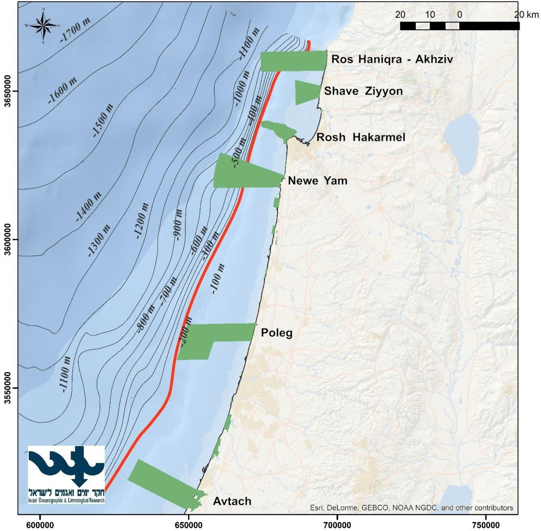
Figure 1 A map of the study region. The red line represents the continental shelf down to a depth of 200 m. The green areas represent the MPAs that were used for this paper.
Ecospace model
The Ecospace model was based on the Ecopath, and Ecosim models described in Corrales et al. (2017a); Corrales et al. (2017b). The Ecopath model describes the ecosystem via 39 functional groups (FGs) that included 19 native and 8 invasive species in the year 1994 (Corrales et al., 2017a; Corrales et al., 2017b; Corrales et al., 2019). Based on this Ecopath model, the time dynamic module Ecosim was constructed and fitted to time series of data from 1994 to 2010, considering the combined effect of alien species, fishing activities and changes in sea surface temperature and primary productivity. In addition, the model successfully simulated the arrival and establishment of invasive species that arrived in the ecosystem after 1994 (Corrales et al., 2017a).
The Ecospace model represents the Levantine Sea area via a 1 km2 grid, with a basemap of 80 columns and 170 rows. This cell size provided a good trade-off between spatial resolution to capture ecosystem dynamics and computational costs. Spatial inputs included bathymetry, relevant classes of substrate, and environmental factors namely water temperature and primary productivity (Table 1). To implicitly capture ecosystem dynamics at depth, temperatures were expressed for two depth ranges: from 0 to 30 m depth for pelagic species, and temperatures near the bottom for benthic species (example in Figure 2). Primary production (PP) was vertically integrated for the upper 30 m. Time series of maps of temperature and PP were downloaded from the Copernicus Mediterranean Sea Physics and Mediterranean Sea Biochemistry reanalyzes at monthly averages (Apicella et al., 2022). These maps were input into the model, at monthly time steps, via the Ecospace spatial-temporal data framework (Steenbeek et al., 2013).
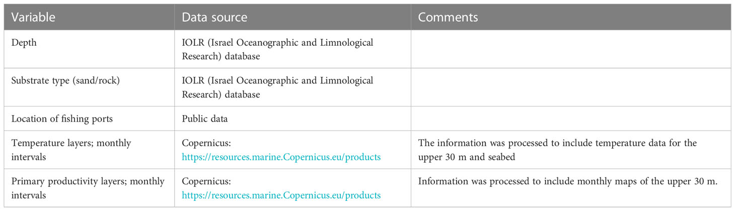
Table 1 The environmental variables used in the model of the Eastern Mediterranean Sea.
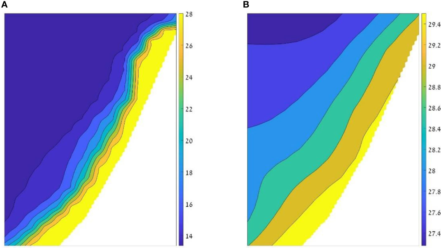
Figure 2 Example of the temperatures input layers for the model. The two layers represent August 2014: (A) temperature layer of the deep layer, adjacent to the bottom with temperatures ranging between 13.3°C (blue) to 29.9 °C (yellow); and (B) temperature layer of the upper 30 m (pelagic zone) in which the values range from 27.2°C to 29.9°C.
In Ecospace, environmental conditions are applied to the living components through functions that express the preferences for, or tolerances to, varying environmental conditions (Christensen et al., 2014a). For the most sensitive species we created these response functions using information from open sources such as AquaMaps (Kaschner et al., 2016), which were complemented with local expert knowledge. For composite functional groups, response functions were aggregated according to the relative proportion of each species’ biomass in the functional group (Appendix 1).
Validation of the model results
To test the results of the model, and to assess its goodness of fit to observed data, we compared our model results to scientific fish surveys. Ecospace was run with temperature and primary productivity (PP) layers of monthly time steps from 1994 (for temperature) and 1999 (for PP) to December 2014 (Apicella et al., 2022). The surveys were conducted in 2012, using trawl nets in two locations, Haifa and Nitzanim, in spring/summer (May, June) and in autumn (October, November) (Goren et al. unpublished data). To enable comparison between the model results and the survey we used the built-in EwE utility that allows extraction of results along transects, assuming that the survey is a straight and narrow line, the model provides results for all groups in the cells included in the transect. We defined three transects at each sample site according to the beginning and end coordinates of the scientific surveys (Figure 3). To calculate the total volume of survey catch, in units of tons per unit area (km2), we converted the catch using trawling distance and the area of the net opening and created a factor which considers the size of the net, distance and towing time that allowed as to convert the model results to survey data. The comparison between the survey results and the model results was conducted for the relevant (benthic and demersal) functional groups according to the following steps:
1. Classification of the species sampled in the survey to the functional groups of the model
2. Conversion of the number of individuals sampled to wet weight biomass (tons)
3. Division of the results to monthly intervals according to the survey months.
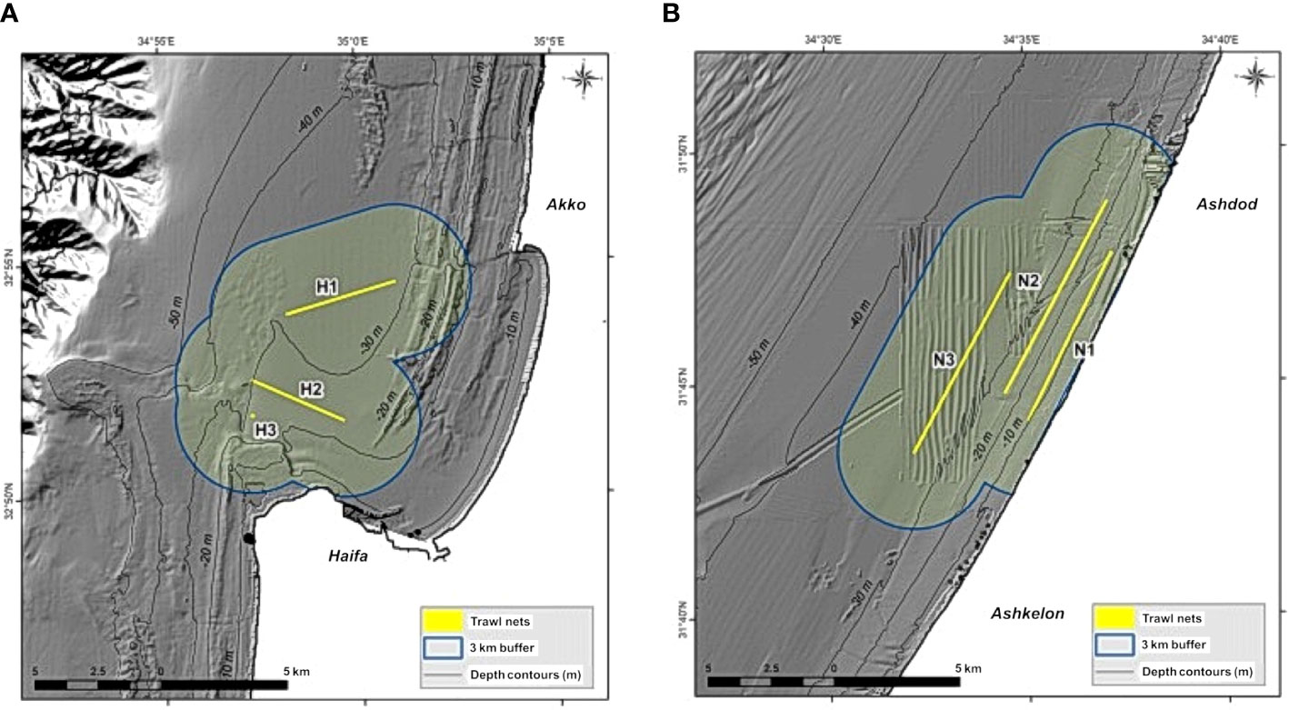
Figure 3 Maps of trawl lines and model calculation areas: (A) sampling area in Haifa Bay, and, (B) sampling area in Nitzanim. The lines represent the sampling transects in the scientific survey; the areas outlined in blue represent the area they cover in the model, representing an area of 1 km2 on either side of the transects (Kanari et al., 2020).
We compared the survey results to the model results and calculated spatial correlations which takes into account the net size, net drag distance and depth between the different groups and between the different months of the survey. The comparison was conducted by determining the relationship between the model results and the survey results, and examining seasonal trends in the surveys and in the model by comparing the catch during the different months in relation to the values in June. Thus, we compared, for example, the ratio between the results in October and in June. In addition, we conducted a visual comparison of the results to aid our examination of the differences between the groups.
Scenarios
Finally, several scenarios were developed and tested to examine the plausible consequences of different management interventions on the ecosystem, the fishing community and the catch, under projected climate change conditions.
Climate change scenarios
To examine the future consequences of climate change and the various management alternatives we used the output from the Med-CORDEX modelling framework (Ruti et al., 2016) under the RCP8.5 scenario. Med-CORDEX is a unique framework where research communities make use of atmospheric, land surface, river and oceanic models in regional climate system models to increase the reliability of past and future regional climate information and understand the processes that are responsible for Mediterranean climate variability and trends. We obtained predictions of sea water temperature from three different sources. We adapted predicted water temperatures for the model region to create monthly temperature layers for the period 2006–2100 for the upper 30 m and for the layer adjacent to the bottom. The use of three different sources allowed us to introduce uncertainty into the temperature inputs (Figure 4). Outputs from regional Med-CORDEX (MC) models were used to drive the Ecospace model under the RCP8.5 emissions scenario (Soto-Navarro et al., 2020):
1. MC1: The first configuration was the coupled CNRM-RCSM4 simulation (Sevault et al., 2014; Darmaraki et al., 2019) that was developed and operated at the Centre National de Recherches Météorologiques (in France). It has an atmospheric resolution of 50 km and an ocean resolution of 9–12 km and 43 ocean vertical levels.
2. MC2: The second configuration was also coupled with a biogeochemical component, the Eco3M-Med (Baklouti et al., 2021). The RCP8.5 projection simulation outcome (Pagès et al., 2020) of net primary production was used in our study.
3. MC3: The third Med-CORDEX ensemble member provided water column temperature evolution under the RCP8.5 climate scenario for this study was the CLMcom-GUF (Model 3) (Bucchignani et al., 2018; Primo et al., 2019) that was developed at the Institute for Atmospheric and Environmental Sciences, Goethe University Frankfurt (Germany), in collaboration with the CLM-Community. It has an atmospheric resolution of 25 km and an oceanic resolution of 12 km. It follows terrain sigma vertical coordinates with 75 layers in the ocean component.
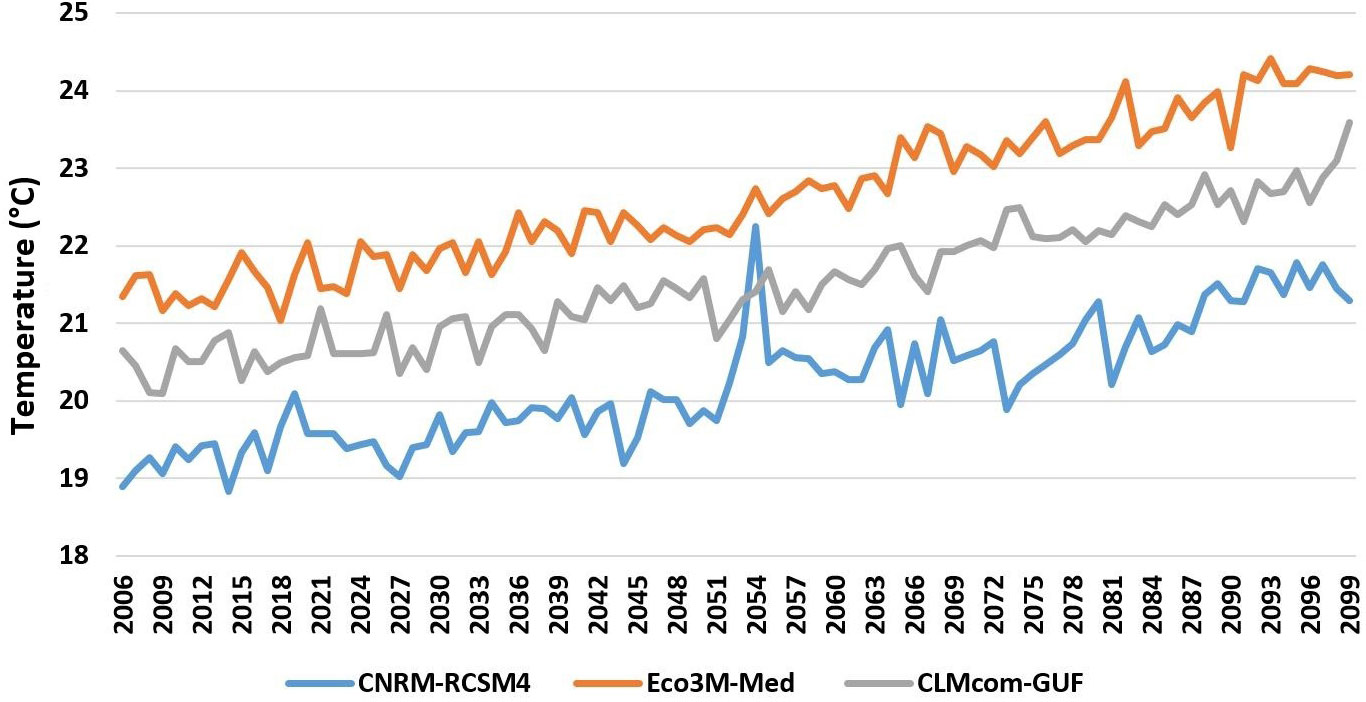
Figure 4 Predictions of the three climate models for the RCP8.5 scenario for increasing sea water temperature in the upper 30 m in Israel’s continental shelf region for the period 2006-2100.
Alternative management options
To examine alternative management options of the ICS region we chose a number of management scenarios, some of which are being assessed by policy makers. The management scenarios were divided into those that restrict fishing for certain periods or regions for different types of fishing fleets, those that examine closure of defined areas to fishing (no-take zones) and their classification as protected areas, and a range of scenarios that combine the different options (Table 2). The following management scenarios were constructed and tested over the period 2006-2100:
1. FM (Fishery management) 1: Closure of the northern part of the maritime region to fishing. The northern region includes expansive rocky areas and unique habitats; therefore, we examined the significance of completely closing it to fishing. The area chosen for closure is greater than that included in the 2016 fishing regulations; the closure stretches from Rosh Hanikra south to Dor Beach.
2. FM2: Closure of a network of nature reserves to fishing (Figure 1). We based our decision on the locations of the nature reserves in the current proposal by Israel’s Nature and Park Authority (NPA) to establish a network of six nature reserves of different sizes from north to south (Seker, 2015). We assumed that these nature reserves would be no-take zones.
3. FM3: Seasonal fishing ban during May and June – this scenario is based on the 2016 fishing regulations, in which the Chief Fisheries Officer can order fishing to be stopped during the breeding season. We assumed a complete ban on fishing during May and June.
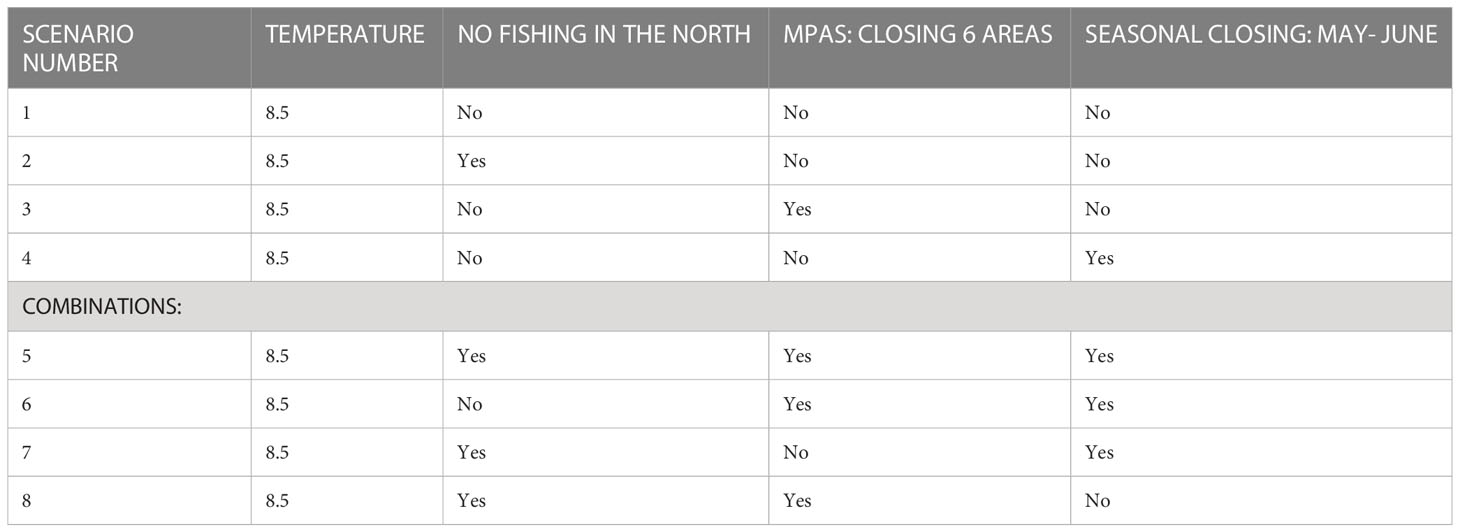
Table 2 Description of the scenarios examined with the ICS Ecospace model.
We further examined a baseline scenario (scenario #1) with no management intervention in the ecosystem. The aim of this baseline scenario was to examine the way the ecosystem fluctuates under the projected future climate change conditions according to the RCP8.5 scenario, with clear increases in water temperature. This scenario did not include changes to fisheries management and served as a basis for comparison with the other scenarios that included fisheries management intervention. All of the scenarios were examined using the model ensemble of the three climate models (MC). All the results of the scenarios were compared to 2020 as a base year since it represents the current period.
The results of the management scenarios presented are an average of the three climate models results. The use of a model ensemble to examine ecological scenarios is becoming more common within the ecosystem modelling community (Jones and Cheung, 2015; Tittensor et al., 2018; Bryndum-Buchholz et al., 2019; Lotze et al., 2019). The use of a model ensemble enables examination of scenarios while accounting for uncertainty associated with the various models and scenarios and increasing confidence in expected outcomes.
Analysis of the scenario results
We used a number of indices to examine the scenario results and the effect of climate change and management options on the ecosystem. Some of the indices, such as biomass and catch, and a range of other indices were calculated by the model (Coll and Steenbeek, 2017; Vilas et al., 2020). The indices included general ecological indices that characterize ecosystems, but also specific indices to characterize fishing.
The indices calculated based on the scenarios results included:
1. Marine Trophic Index (MTI) – represents the average trophic level of all components in the catch with TL equal or higher to 3.25 (Kleisner and Pauly, 2011; Coll and Steenbeek, 2017).
2. TL catch – an index that quantifies the trophic level of the catch; it serves as an indicator of the extent of exploitation of the fish resource in the sea. Use of this index is based on the assumption that we fish down the food web (Pauly et al., 1998), meaning, the higher the fishing pressure, the lower the trophic level of the catch (Shannon et al., 2014).
3. Kempton’s Q – The Q index is proportional to the inverse slope of the species-abundance curve arranged by trophic levels and is a proxy of ecosystem biodiversity (Coll et al., 2016a).
4. Shannon diversity – an index of species diversity in the ecosystem that enables comparisons over time (Coll et al., 2016a).
Scenario results included annual results for biomass, catch, and the various indicators. The results were compared to the scenario without management intervention to identify the effect (positive or negative) of each management option. In addition, to simplify the analysis of all the information produced by running the scenarios, we grouped the model’s FGs into a number of broad groups (fish, local fish, invasive fish, invertebrates, zooplankton, total catch, local species catch, invasive species catch). The division of the broad groups into invasive and local species allowed us to analyze ecosystem fluctuations more clearly and follow the distribution of invasive species and their function in the ecosystem. The layers of information produced by the model were analyzed and visualized at each time step using Matlab, version R2021b. In addition, we created maps of the results in order to examine the spatial distribution of the FGs and broad groups. The results were analyzed using a number of approaches:
1. Temporal dynamic comparison (using annual time steps) of the biomass of the broad groups and calculation of the relationship between the scenario results and the base scenario results.
2. Comparison among scenarios of the average value of each of the indicators throughout the model space. We conducted a relative comparison of the indicators of all scenarios, under the three different climate change drivers.
3. Examination of the contribution of defined protected areas (nature reserves) on the conservation of the local species within the nature reserve.
In order to evaluate the possible benefits of the nature reserves, we calculated the biomass of the different groups in the nature reserve and compared it to the regions outside the protected area and to the scenario without the nature reserves. The examination was done by dividing the cells such that we could isolate the cells comprising the nature reserves and the region next to the nature reserves in the scenario results. We calculated the area of this defined region, and according to its size we calculated the average biomass per km2 in order to compare different regions. The next step was to compare what exists within, and adjacent to, the Rosh Hanikra Nature Reserve. The choice to present this region stems from the fact that Rosh Hanikra Nature Reserve is an active, monitored, existing nature reserve; thus, we can compare the model results to the insights from the surveys conducted by the NPA in the nature reserve.
Results
Model validation
We compared the survey results with the results produced by the model for a transect analogous to the survey region. Since there is variation between sites and among seasons, we conducted the comparisons for each site separately. Overall, there was a good fit of the biomass estimates for the different groups between the surveys and model results, with differences ranging between -15% to +30% on average over all months and sites. Nevertheless, the results were not uniform and there were differences between sites and among groups.
We obtained a 95% correlation between the survey and model biomass results for the different groups in Haifa, averaged over all months (Figure 5). In most groups, the correlation was very high; however, there were exceptions, such as “earlier invasive dem. fish” for which the model predicted notably higher biomass than was obtained in the survey during May (0.2 vs. 0.01 t/km2, respectively) and June (0.2 vs. 0.05 t/km2, respectively).
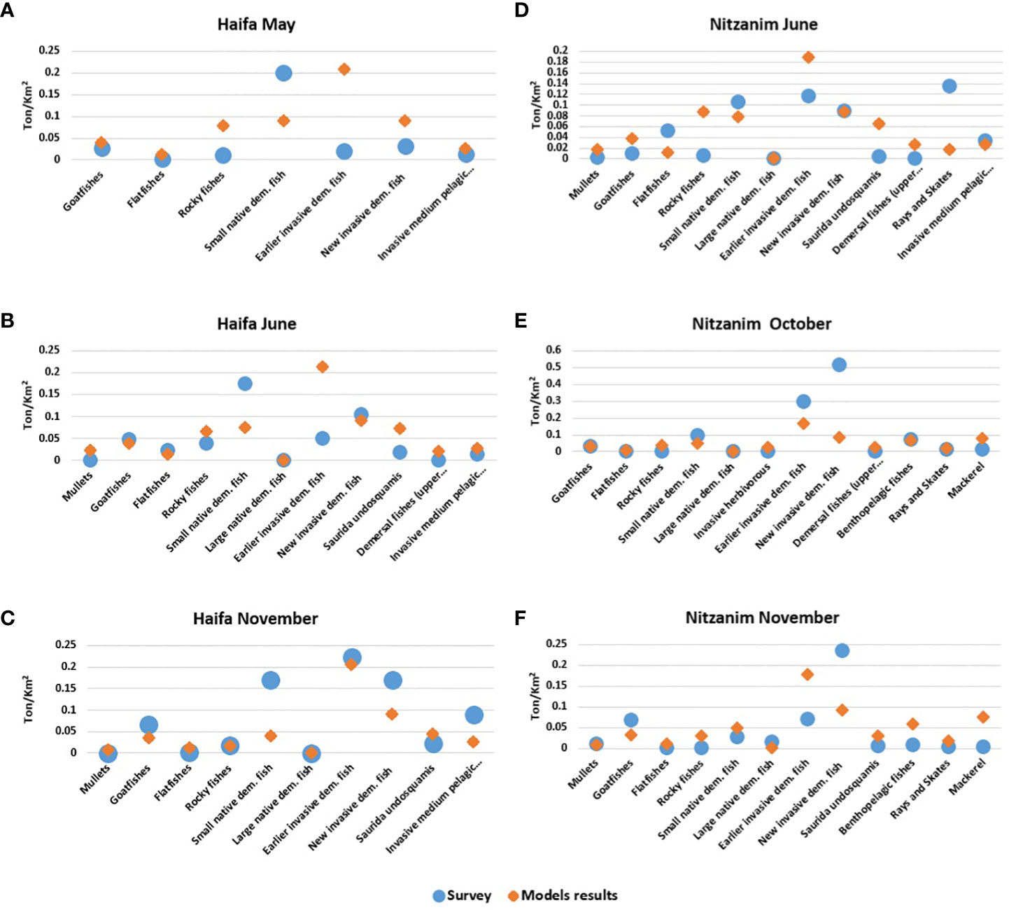
Figure 5 Comparison of model results (orange) and survey results (blue). (A-C) Haifa: May, June, and November; (D-F) Nitzanim: June, October, and November. The numbers represent biomass in t/km2.
For the Nitzanim site, the differences were of +20% on average between the survey and the model results for all groups and all months (Figures 5D-F). These results also showed that the correlation was high for nearly all groups. However, here too, there were exceptions, for example “new invasive dem. fish” which demonstrated greater differences, in October, with 0.5 and 0.08 t/km2 for the survey and model, respectively, and in November, when the survey results indicated 2-fold higher biomass than model predictions. We also found a difference for “rays and skates” at Nitzanim, in May, with 0.13 and 0.01 t/km2 for the survey and model, respectively.
Overall, there was a high correlation between the survey and the model results when examining the seasonal fluctuations. For example, for Haifa, the comparison between November and June shows that eight of the nine functional groups exhibited almost perfect correlation between the model and the survey with correlation values (R) of 94%. Similar results were obtained for seven of the nine groups at Nitzanim for the comparison between November and June (Figure 6). However, analysis of the outlier groups in May and June in Haifa highlighted the differences in the seasonal variation. The range of seasonal variation in the model results reached 20%, while in the survey results the variation in the extreme cases reached 90% (Figure 6A); this difference in range was observed for five groups. In contrast, there was a large degree of similarity between the model and survey results, in the comparison between November and June in Haifa; eight groups had a large degree of similarity (25-88%) between the November and June results, while only one group exhibited a significant difference of 450% of Rocky fishes (Figure 6A). Even in the case of comparing relationship between November and June in Haifa, to the survey results, only one group had difference between seasons of to 600% (Earlier invasive dem. Fish) while the model results had differences of up to only 60% between seasons (Figure 6B). The results for Nitzanim were similar; the comparison between October and June showed a high correlation (average of 75%) in six groups and differences of up to 600% in the survey results for one group, while the model results demonstrated changes of up to 50% (Figure 6C). The comparison between November and June in Nitzanim showed the same trend with a high correlation (average of 80%) in seven groups and a low correlation (25-16%) in two groups also, the survey results varied between seasons by up to 600%, (Figure 6C) while the model results varied seasonally by up to only 70% (Figure 6D).
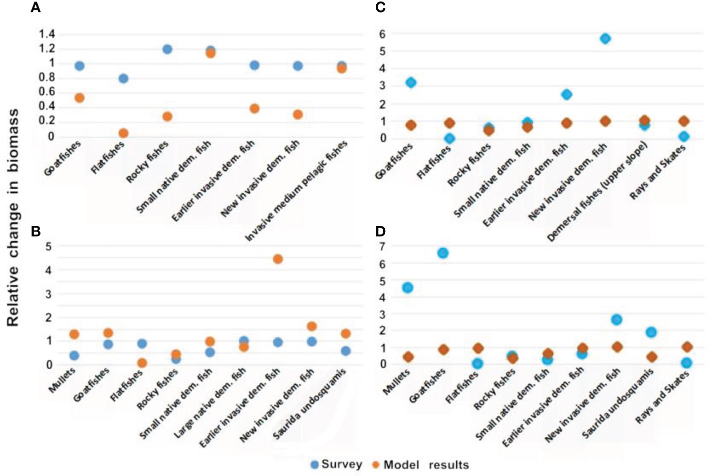
Figure 6 Comparison of seasonal differences in the model results and survey data: (A) relationship between June and May in Haifa; (B) relationship between November and June in Haifa; (C) relationship between October and June in Nitzanim; and (D) relationship between November and June in Nitzanim. The Y-axis is a relative scale of biomass change. The X-axis are the groups which were found in the month the survey was conducted.
Scenario results
Baseline scenario- climate change
In general, outputs from the Ecospace model with the three-climate change driven ocean models resulted in similar trends of change in the food web, though the level of intensity varied between models. Driving Ecospace with the output from MC 1 resulted in the highest biomass results, producing 23% more biomass that the other two models. Driving Ecospace with output from MC 2 and 3 resulted in similar biomass levels (Figure 7).
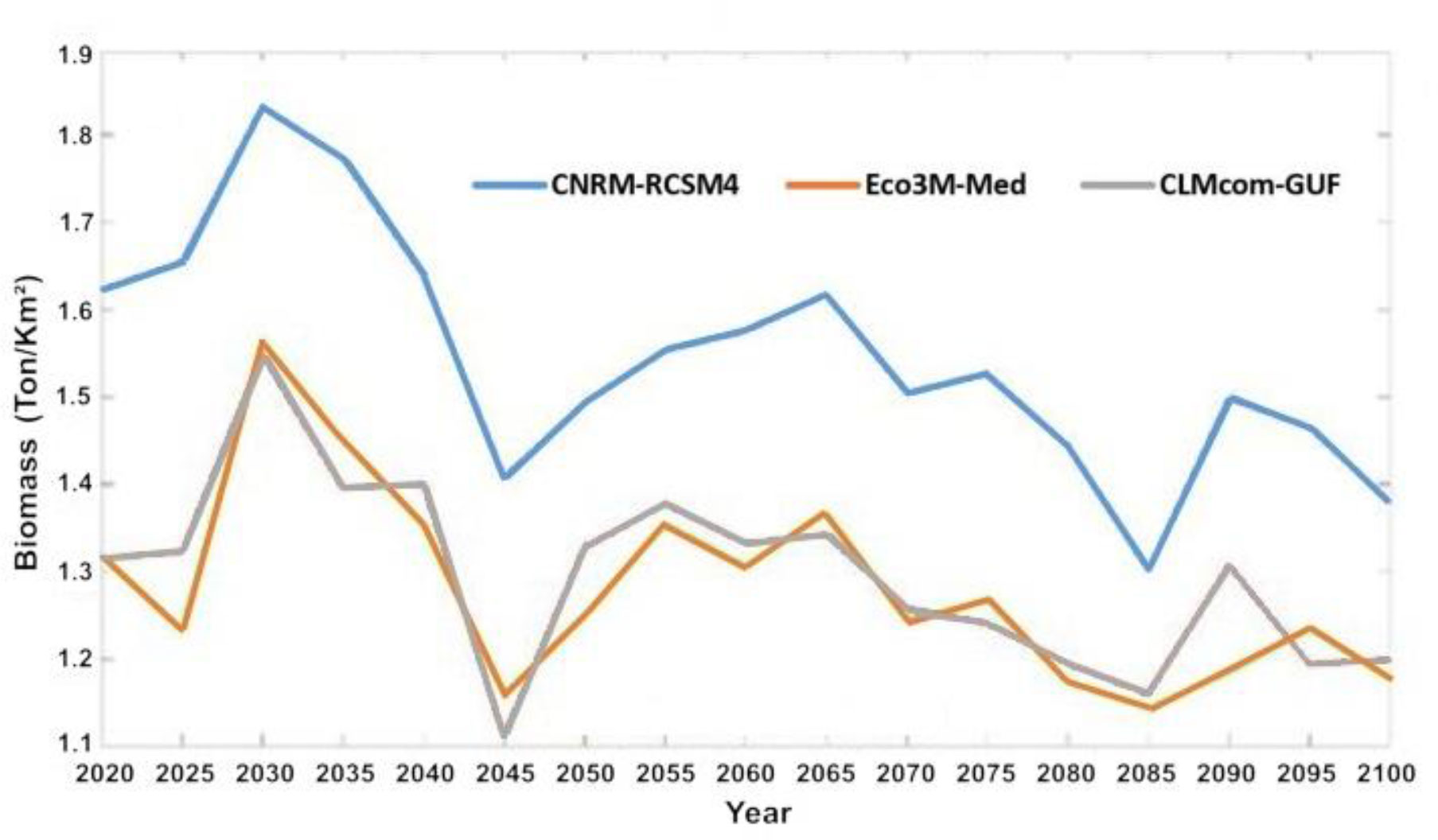
Figure 7 Average biomass of fish in ton/km2 for entire model domain under the three selected ocean models: MC1 (CNRM-RCSM4), MC2 (Eco3M-Med) and MC3 (CLMcom-GUF).
The results of the baseline climate change scenario (Scenario 1) demonstrated an average decrease in biomass of 16% (from 1.4 to 1.2 ton/km2) for all the fish in the ecosystem over the course of the scenario (Figure 8A). This result combines a decrease of 37.5% in the biomass of native fish (Figure 8B) and an average increase of 26% in the biomass of invasive fish (Figure 8C). Even the total catch, comprising local species and invasive species, demonstrated a decrease of ca. 11% from 0.3 to 0.27 t/km2 (Figure 8D).
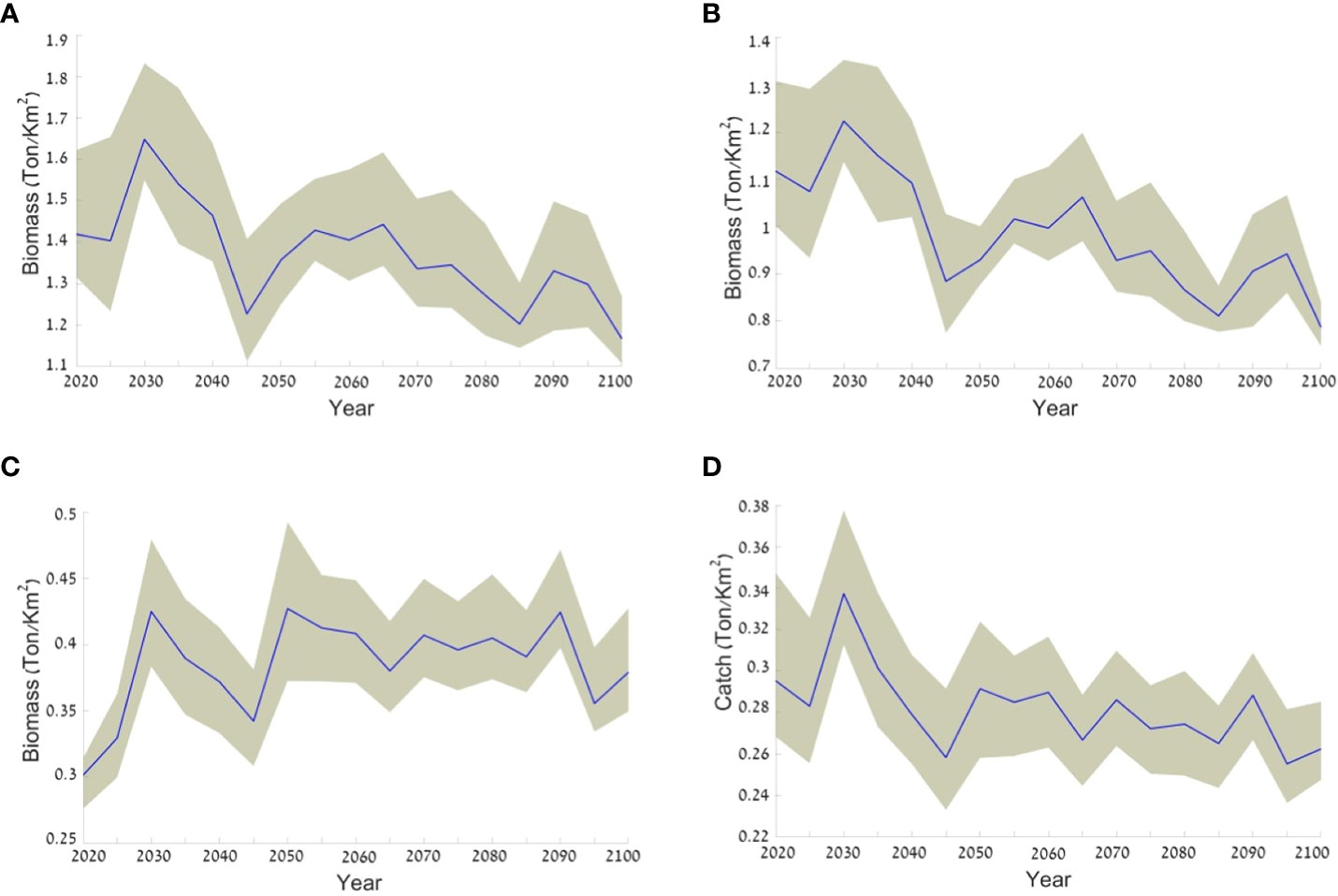
Figure 8 Expected changes in the biomass of different groups according to the baseline climate change scenario (Scenario 1). The average is represented by a blue line and the range of values resulting from using the three climate models is represented by the grey area surrounding the average line. The figure presents results for (A) all fish groups biomass; (B) native fish biomass; (C) invasive fish biomass; and (D) the total catch. Values are in ton/km2.
Climate change scenarios and management steps
In contrast to the baseline scenario, we found a marked increase in the biomass of native fish when we implemented all regulatory measures, namely, limiting fishing during the breeding season, and creating no take zones by networks of nature reserves or by closing the northern region to fishing (Figure 9). Scenario 5, which represents this option, demonstrated a rapid increase and by 2020, 15 years after the start of the simulation there was a 25% increase in the biomass of native species, with respect to the baseline scenario, and an increase of up to 45% by 2100. In contrast, limiting fishing during the breeding season alone (Scenario 4) led to a moderate (5%) increase in biomass of native species by 2020, and only ca. 2% by 2100 (Figure 9).
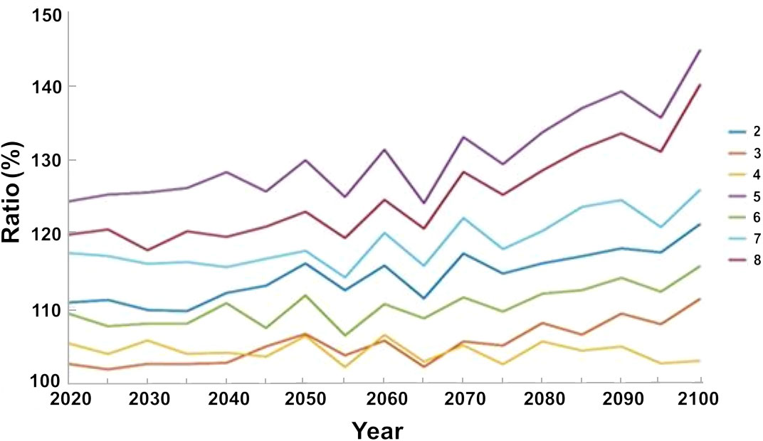
Figure 9 Percent variation in the biomass of native species under the different management scenarios (listed in Table 2) with respect to the baseline scenario (year 2020). The results are the average of the three ocean models.
The maximum decrease in the biomass of invasive species was achieved when all the management steps were implemented (Scenario 5), namely, limitations to fishing during the breeding season and exclusion of fishing in nature reserves and in the country’s north. Under this scenario, the biomass of the invasive species decreased by ca. 28% with respect to the baseline scenario until 2020, and by ca. 23% until 2100. Under the scenario of excluding fishing in the country’s north (Scenario 8) the biomass of invasive species decreased by ca. 23% with respect to the baseline scenario until 2020, and by ca. 20% until 2100. The smallest decrease in the biomass of invasive species occurred under the scenario that only limits fishing during the breeding season (Scenario 4), with a decrease of ca. 10% with respect to the baseline scenario until 2020; however, by 2100 the biomass values did not differ from those of the baseline scenario (Figure 10).
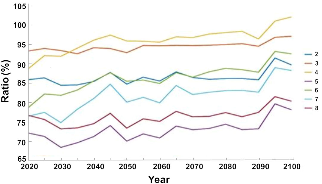
Figure 10 Percent variation in the biomass of invasive species under different management scenarios (listed in Table 2) with respect to the baseline scenario that does not include management steps. The results are the average of the three ocean models.
Analysis of the expected changes in the catch under different management steps indicate that the management steps will not result in an increase in the total catch relative to the baseline scenario for the entire simulation period. Some management steps, however, minimize the impact on the size of the catch and the expected decline is smaller than observed without management measures. While under the base scenario, without any management measures there is about 20% decline in catch by 2020 and about 32% by 2100, there are minimal declines under scenarios 3 and 4. Under both scenario 3, i.e. creation of no-take zones, and scenario 4, i.e. a fishing ban during May and June, the breeding season there is average decline in catch of 5% by 2020 with a variation of 3.4% for scenario 3 and for scenario 4, 5% by 2100 with respect to the baseline scenario. In scenario 5, in which all management steps were implemented the total catch was the lowest with respect to the baseline scenario, with an average decrease of 25% by 2020 and a decrease of 28% by 2100 with variance of 13.2% from 2020 to 2100 (Figure 11).
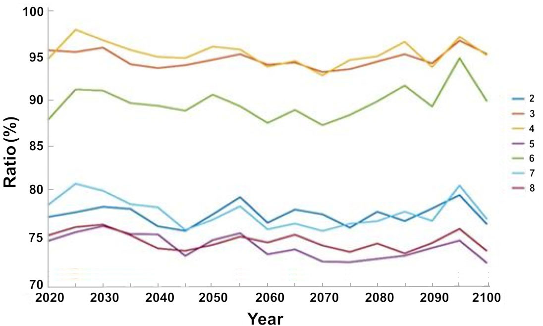
Figure 11 The change in the total catch under the different management scenarios with respect to the baseline scenario. The results are the average of the three ocean models.
Effect of management actions on the ecosystem
In all of the scenarios tested, the variation in the Mean Trophic Index (MTI) of the ecosystem was not large, ranging from 3.65 to 3.73, which was lower than the MTI of the baseline scenario. In all scenarios there was a clear trend of an increase in MTI over the period of the scenarios, ranging from 3.63-3.66 in 2020 to 3.68-3.73 in 2100 in the different scenarios (Figure 12A).
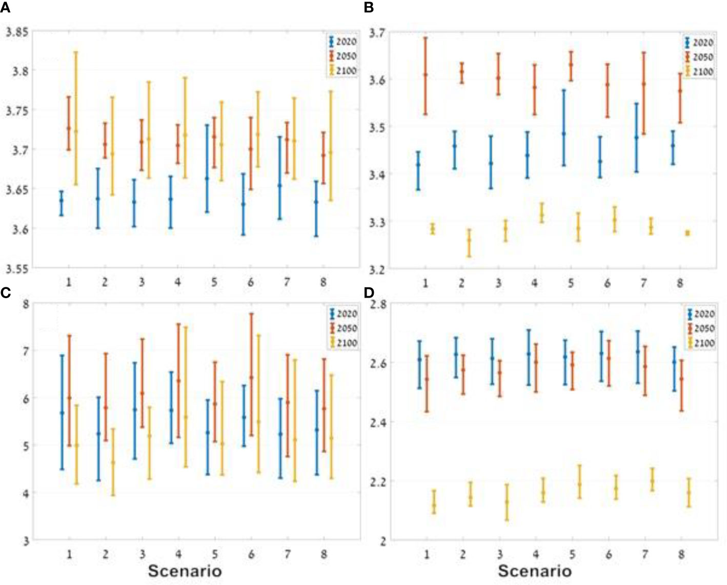
Figure 12 Results of the indicators for the three ocean models under the different management scenarios. The horizontal axes represent the different scenarios (1-8) and the vertical axes represent the values of the different indices: (A) MTI (mean trophic index); (B) total catch; (C) Kempton’s Q; and (D) Shannon diversity index. The vertical lines represent the distribution of the results of the three ocean models around the average (dot). The blue line represents the results for 2020, the red line represents the results for 2050, and the yellow line represents the results for 2100.
Analysis of MTI of the total catch indicates a marked increase from 2020 to 2050, followed by a decrease to 2100. The management scenario that excludes fishing in the country’s north and in nature reserves (Scenario 5) produced the highest MTI in 2020 and 2050. In contrast, the lowest MTI in the year 2100 occurred in the scenario that only excluded fishing in the country’s north (Scenario 2, Figure 12B).
The Kempton’s Q results show a small degree of variability between results based on the different ocean model forcing, but a number of patterns did emerge. The lowest diversity, in 2020, when there was no fishing in the north (Scenario 2), i.e. the effect of fishing and climate change on the ecosystem is the lowest for the three examined time periods. And while scenario 2 exhibited low Q values for all time periods it was not the lowest in 2100. Scenario 4, in which seasonal exclusion of fishing was implemented, the index was the highest during all three time periods. In all scenarios, including the baseline scenario, the index increased up to 2050 and then decreased towards 2100. Since this occurs under all scenarios, it appears that up to 2050 the effect of climate change overrides any effects of management scenarios with respect to this index (Figure 12C).
Under all scenarios there was a decrease in the Shannon index over time, with a stronger decrease between 2050 and 2100 (Figure 12D). In 2100, the baseline scenario (Scenario 1), without management steps, had the lowest Shannon index value, while the highest value was found under scenario 7 in which fishing was banned in the country’s north and there was a seasonal ban on fishing in general. The results show two notable differences in diversity index values in relation to the other indices. The first, the larger difference in values between 2050 and later periods (2100), the second, was the low variability between the different management scenarios (<0.1) indicating that perhaps the index may not be sensitive enough to the management scenarios examined in this study.
The Achziv (Rosh Hanikra) nature reserve
To examine the benefits of nature reserves to the ecosystem, we chose the Achziv Nature Reserve as a case study. In order to evaluate the effectiveness of the reserve, we used the results from the scenario that included only closures of nature reserves (Scenario 3). These results indicated that within the reserve the fish biomass was higher than outside the reserve. In addition, there was a higher biomass of native species and lower biomass of invasive species within the reserve though the variation in the invasive species group was higher than the native species group and the fish group (Figure 13).
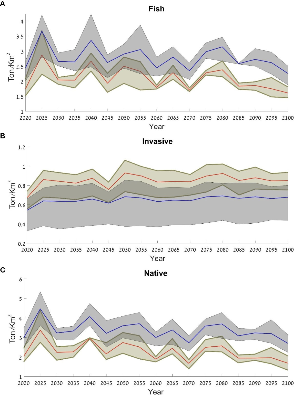
Figure 13 Average fish biomass for the three ocean models assuming closure of protected areas (Scenario 3), in and around Achziv Nature Reserve: (A) all fish species; (B) invasive species; (C) native species. The blue line represents the results within the reserve and the red line represents the results outside of the reserve. The results are expressed as t/km2.
Discussion
There is much uncertainty concerning the severity of the climate change that is projected to take place over the coming decades and the impacts of the possible changes on aquatic ecosystems. In this study, we tested the possible consequences of climate change on the ecosystem of the Eastern Mediterranean based on the more severe IPCC RCP 8.5 scenario (Smith et al., 2014) (Pagès et al., 2020).
In light of the uncertainty in models, extensive use has been made of model ensembles for testing scenarios. In the current study, we implemented the model ensemble approach in order to include the range of uncertainty regarding the future environmental conditions that will affect the ecosystem according to our scenarios. The use of model ensembles, though common in climate studies, is still rare in respect to all aspects of implementation of marine spatial ecological models (Steenbeek et al., 2021). There are, however, a number of examples such as (Bourdaud et al. (2021) who used RCP2.6 and RCP8.5 in order to analyze the impact on species distribution using an ecological model and additional studies at the global scale (Lotze et al., 2019; Coll et al., 2020; Tittensor et al., 2021).
We used the output from three different climate-ocean models (Darmaraki et al., 2019; Pagès et al., 2020) in order to test the impact on the ecosystem. The approach we used allowed us to test a possible response of the ecosystem under a range of future conditions. In this case, similarity in the trends of responses to environmental changes and management steps reinforces our results for drawing conclusions.
The results of the basic climate change scenario (Scenario 1) under RCP8.5 pointed to a number of trends in total biomass of fish, the size of the fish catch, and changes in the biomass ratio between invasive and native species. In this scenario, the fish catch decreased on average by ca. 11% and the average biomass of all the fish in the ecosystem decreased by 16% throughout the period of the scenario. The results are consistent with global projections that show a reduction in the biomass of a variety of species under RCP 8.5 Tittensor et al. (2021). Furthermore, our scenario showed an average increase of 26% in the biomass of invasive species, but a 37.5% decrease in the biomass of native species. These results support the trends identified in other studies conducted in Israel, indicating migration of native species to regions with colder, deeper water, some of which are located outside our model domain (Chaikin et al., 2022). The results also illustrated the impact of climate change not only on biomass and fish catch but also on species composition. Higher temperatures, according to the results of the basic scenario, led to an increasing trend in the relative abundance of invasive species in the community, similar to the phenomenon taking place in other regions of the world (Geburzi and McCarthy, 2018). This corresponds to previous studies in our region that show the relationship between the increase in sea water temperature and the biomass of the invasive and local species (Corrales et al., 2018; Corrales, 2019).
The increased water temperature also had an impact on the fish catch. The catch displayed a decrease in size, and also a change in composition, such that it included a large proportion of invasive species and less native species. This is similar to the phenomenon observed in the northern Pacific Ocean where marine heatwaves are worsening the impacts of climate change on 795 fisheries. This is due to the increased ocean temperatures causing changes in the distribution and abundance of fish, leading to economic and ecological consequences for these fisheries (Cheung and Frölicher (2020); Cheung and Frölicher (2020).
Ranking the results of each scenario is a way to analyze the results and attempt to find the management steps that maximize the benefits. Based on the results of the scenarios, we assigned a score to each of the scenarios based on the degree of its contribution to the increase in the biomass of local species, the decrease in the biomass of the invasive species and the changes in catch. Analysis of the scenarios revealed that all management actions improved the state of the native species, caused a decline in the biomass of invasive species and preserved fish catch. Nevertheless, a number of management actions were noticeably more effective than others (Table 3). Scenario 5 provided the best desired results for both the ecosystem and fish catch. This result was achieved by combining all of the management options, namely, combining no-take zones protected from fishing, cessation of fishing in the north and cessation of fishing during May and June in other areas. The significance of this scenario was the creation of a network of protected areas in which the native species can thrive, thus minimizing their displacement by invasive species, as well as complete cessation of fishing for two months to enable the fish populations to survive. However, scenario 5 displayed one of the lowest scores for the fish catch; this stemmed from the creation of no-take zones as well as the complete cessation of fishing for two months.
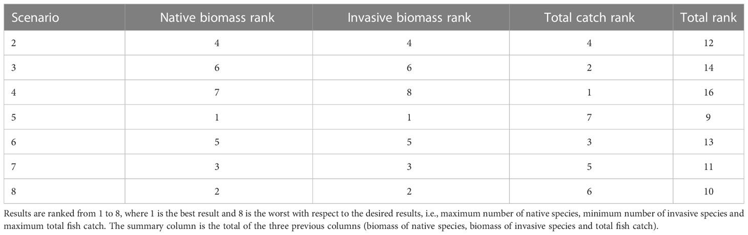
Table 3 Ranking of the results of the management scenarios, and their impact on native species, invasive species and the fish catch.
Another management action that had a positive effect on the fish catch was cessation of fishing during May and June (Scenario 4). The effect of this step on the fish biomass in the long run was not surprising since after cessation of fishing, great effort is made to “make up for lost time”, as reported from other locations (Sterner, 2012). Nevertheless, this management step had almost no benefits on the native species; thus, from an ecological perspective it does not contribute to protection of the ecosystem.
It appears that creating no-take zones that enable native species to survive undisturbed as well as steps to restrict fishing (e.g., Scenario 8) facilitated protection of the ecosystem and had some level of benefit to the fish catch. Implementation of this policy requires an effort on the part of the government, since creating no-take zones and restricting fishing to certain times of the year attract great opposition from the fishing community, resulting in conflicts. However, the results of the scenarios clearly show that implementation of such steps is one of the best options to improve the catch and the ecosystem (e.g., Scenarios 3 and 6). These results are in line with reports on the implementation of management steps in other locations around the world (Vilas et al., 2020; Hoppit et al., 2022).
We used ecological indicators to test the consequences of future changes on the ecosystem itself (Susini and Todd, 2021). To understand the impact of management steps on the entire ecosystem, we calculated, for each indicator, the average value over the duration of the scenarios. The advantage of this approach was that it provided a general perspective of the system, it discounts, however, the spatial variation between different locations. Overall, in the baseline scenario all the indicators pointed to a decrease in ecosystem functioning between 2050 and 2100. This may be related to the constant increase in sea water temperature which in some climate scenarios become more intense towards the end of the test period. Rising temperatures are expected to impact ecosystem functioning (Bourdaud et al., 2021).
Examination of MTI showed almost no difference between the management scenarios (despite differences in the proportions of native and invasive species). From this we can conclude that ecologically, there is a phenomenon of displacement of native species by invasive species that take their place in the trophic level of the food web. This is in line with previous studies (Corrales et al., 2017a; Corrales et al., 2017b; Corrales et al., 2018; Corrales, 2019) that indicated displacement, mainly of crabs and shrimps. Nevertheless, the spatial extent of the model is limited to a depth of 200 m, thus, our model cannot detect a situation where native species move to greater depths in search of better thermal conditions or because they have been displaced by invasive species.
Indices of species diversity indicated changes in ecosystem functioning (Goswami et al., 2017). Examination of Kempton’s Q, which tests the biodiversity (Ainsworth and Pitcher, 2006; Coll and Steenbeek, 2017) shows that Scenario 2, in which the northern zone was closed to fishing, is the scenario with the lowest biodiversity. This result is not surprising, since stricter restrictions on fishing lead to more biomass across the food web, resulting in lower index values. From a management perspective, we can conclude that closing the northern zone is more effective than creation of no-take zones. However, since this is not the decision makers’ sole aim, this step should be considered in the light of other objectives.
Evaluating expected changes in diversity based on the Shannon index highlighted a number of patterns. Firstly, the notable decline in index values between 2050 and 2100. In all management scenarios, this is as a response to climate change. Secondly, the low variability between results based on the three different ocean models, and, thirdly, was the low variability between the different management scenarios. The low variability between the three models and scenarios reflect the displacement phenomenon described in this and other studies (Goren et al., 2016; Corrales et al., 2017a), where invasive species fulfill the same role in the ecosystem as the native species they replace. This insight is reinforced by the fact that the changes in the trophic level of the fish catch are also relatively small; in other words, we also see replacement of native species by invasive species in the fish catch. This has already been taking place for some time and is expected to continue into the future.
One of the most common management steps for protecting fish populations and ecosystems is the declaration of nature reserves (Dimitriadis et al., 2018; Grorud-Colvert et al., 2021). Currently, the option of declaring a number of nature reserves along Israel’s Mediterranean coast is being considered, with the aim of protecting native species, unique species and keystone species (Seker, 2015). However, we must ask whether the reserves will fulfill their role under projected climate change. We chose to focus on the results of the scenarios for Achziv Reserve because it is an active, declared reserve, and many surveys have been performed both inside and outside of the reserve to monitor ecosystem dynamics. The model results indicated that the reserve is fulfilling its role: the total number of fish species and the number of native species inside the reserve exceed the numbers in the area around the reserve, while the number of invasive species is lower inside the reserve than outside of it. These results are in line with the results of the abovementioned surveys (NPA, 2015) and other studies in the Mediterranean (D’Amen and Azzurro, 2019) and in Israel in places where there is continuous monitoring of protected areas compared to what happens outside the protected area (such as the Achziv reserve in the northern part of the territorial waters in Israel). It seems that there is an increase in the amount of local species inside the reserve compared to the area outside (Frid et al., 2022). This observation also indirectly verifies the model.
Analysis of the scenario maps results revealed that in areas adjacent to nature reserves there is an increase in the fish catch (Appendix 1/Figure A3). These results are not surprising and are in line with the phenomenon known as spillover or “fishing the line”, where fishermen wait at the edges of the nature reserves and enjoy an abundant fish catch that comes from the reserve (Kellner et al., 2007; Nillos Kleiven et al., 2019; Grip and Blomqvist, 2020). Examination of the fish catch maps from different years showed that in scenarios with implementation of nature reserves there are several main zones with unusually high fish catches. One is in the northern part of the ICS, between three nature reserves, while the other is in the center of the country, north of a large nature reserve (Appendix 1/Figure A3).
The detection of areas with a large fish catch led to the idea of creating designated fishing zones. Currently, the continental shelf is under a range of pressures from a large number of uses. Fishing zones are usually those left after omitting all of the zones in which fishing cannot take place. As far as we know, the idea of creating designated fishing zones in Israel is innovative and it is based on the idea of Ramírez-Luna and Chuenpagdee (2019); Ramírez-Luna and Chuenpagdee (2019) which indicated the development of such areas for Latin America and the Caribbean for small-scale fishing that can support the preservation of this activity alongside provision of fish from the sea. Establishment of such zones can be integrated into spatial planning maps that restrict the other users and allow only fishing or other activities that do not interfere with fishing. The location of these zones adjacent to nature reserves will allow the fishermen to take advantage of the fish catch that develops inside the reserve and trickles out.
Verifying the results of a spatial ecological model is not trivial. As ecological models have developed, the statistical methods designed to test the quality and accuracy of the model results have also developed. Hipsey et al. (2020); Hipsey et al. (2020) suggested an approach that can be used to validate the results of ecological models and mainly to ensure the appropriate use of a model for scenario testing and application as a management tool. The validation process provides tools designed to test the results and identify situations where model require further development or calibration. The state validation processes, as presented by Hipsey et al. (2020); Hipsey et al. (2020), compares simulated state variables, such as biomass or fish catch, and compare them to the range of expected values in reality, based on monitoring, surveys and sampling. This method is the most common form of model verification, and indicates the level of reliability of the results, particularly those models required for decision-making processes (Link, 2021). The ICS Ecosim model underwent state validation (Corrales et al., 2017a). In this study we implemented spatial state validation based on the surveys conducted in two regions over several seasons. In addition, we perform a restricted form of system-level emergent properties validation (Hipsey et al., 2020) as can be seen in the similar patterns that emerged from studying the impact of the Ackziv nature reserve on the fish communities. Validation of spatial ecosystem models is uncommon and challenging (Steenbeek et al., 2021). And indeed there have been very few cases of validation of Ecospace models (e.g. (Grossowicz et al., 2020); in some studies the results of species distribution maps were compared to distribution models using statistical tools (Coll et al., 2019).
In order to verify the spatial model, we compared the results of the scientific surveys to the results of the model along a defined transect. The aim was to test the reliability of the model both in locations with different characteristics (Haifa and Nitzanim) and during different months (May, June, October and November); thus, the validation was performed across both the spatial and temporal (seasonal) dimensions. The results from our validation demonstrate that the model was successful in simulating most of the functional groups in the model, in both locations, and in each of the months, with average deviations of -15% to 30% between the model results and the survey results. However, in this study, due to a lack of available data, we performed the comparison for only one year. In the future it is imperative to use the same method to compare the results for additional years.
The seasonal comparison between the survey results and the model results was performed with respect to June in both test locations. The results show that all four cases demonstrated a high correlation between the model results and the survey results for most groups; only one group (earlier invasive dem. Fish) presented a noticeable difference between the model results and the survey results. Due to the sampling methodology (trawling) used in the survey, it is possible that the large differences observed between the surveys and model results are a consequence of the sampling method used.
We recognize that the modelling complex contains significant sources of uncertainty that we did not yet address in this study. The eastern Mediterranean will likely experience additional species invasions, and when available, different climate forecasts that exceed the 8.5 emission scenario in severity should be considered. Additionally, assumptions in the EwE parameterization are subject to uncertainty that may affect model predictability. Follow-up studies should systematically assess these sources of uncertainty (Steenbeek et al., 2021) once the technological framework required to perform such assessments is available (Steenbeek et al., In prep).
Climate change is happening now and the impact of rising sea temperature on the ecosystem has already been recorded and demonstrated through a number of studies in our region and in other regions around the world (Herut, 2021; Tuel and Eltahir, 2020). Consequences of the climate changes occurring in our region are reflected in the need for native species to adjust the range of temperatures in which they reside. In addition, invasive species that invaded the region, and that are adapted to the higher range of temperatures in the Red Sea, are successfully colonizing and inhabiting the shallow, warmer waters of the Israeli continental shelf (Arndt et al., 2018). In addition, invasive species that are not currently known to us in the study area may arrive and change the dynamics of the ecosystem and the fishery. These changes cannot be predicted, so it will be necessary to examine the model’s products and policy recommendations from time to time and according to the changes in the ecosystem.
By combining an ecological model with climate change scenarios for the purpose of testing different management scenarios, we demonstrate the variability of the ecosystem as a response to different management scenarios, and provide decision makers with tools for selecting the most suitable management measures to mitigate possible climate effects on the ecosystem.
Data availability statement
The original contributions presented in the study are included in the article/Supplementary Material. Further inquiries can be directed to the corresponding author.
Author contributions
EO, and GG conceived the study. XC provided the data for the Ecosapce model. JS, MC, SH helped in model construction and testing. MG provided data and knowledge on the ecosystem. YA, NS, helped in data and spatial layers preparation. All authors contributed to the article, reviewed the manuscript and approved the submitted version.
Funding
This work was funded by the H2020 European project Ecoscope under Grant Agreement ID 101000302, with Grant Agreement ID 101000302 and by the Israeli Ministry of Energy in a grant to GG. XC was supported by the Spanish National Program Juan de la Cierva-Formación (MCIN / AEI / 10.13039/501100011033 FJC2020-044367-I) funded by the Government of Spain (Ministry of Science and Innovation (MCIN) and the State Research Agency (AEI)) and the European Union (NextGenerationEU/PRTR).
Acknowledgments
We thank Dr. Samuel Somot for generously sharing CNRM-RCSM4 temperature fields from simulation conducted under the Med-CORDEX ensemble and express our deep appreciation to prof. Mélika Baklouti for sharing her time and work in providing simulated primary production fields from the Eco3M-Med model. We thank Dr. Nir Stern from IOLR for his insights and comments. MC acknowledge partial funding from European Union’s Horizon 2020 research and innovation programme under grant agreement No 869300 (FutureMares) and No 101059877 (Ges4Seas), and the institutional support of the ‘Severo Ochoa Centre of Excellence’ accreditation (CEX2019-000928-S).
Conflict of interest
The authors declare that the research was conducted in the absence of any commercial or financial relationships that could be construed as a potential conflict of interest.
Publisher’s note
All claims expressed in this article are solely those of the authors and do not necessarily represent those of their affiliated organizations, or those of the publisher, the editors and the reviewers. Any product that may be evaluated in this article, or claim that may be made by its manufacturer, is not guaranteed or endorsed by the publisher.
Supplementary material
The Supplementary Material for this article can be found online at: https://www.frontiersin.org/articles/10.3389/fmars.2023.1155480/full#supplementary-material
References
Abdou K., Halouani G., Hattab T., Romdhane M. S., Lasram F. B. R., Le Loc’h F. (2016). Exploring the potential effects of marine protected areas on the ecosystem structure of the gulf of gabes using the ecospace model. Aquat. Living Resour. 29, 202. doi: 10.1051/alr/2016014
Ainsworth C. H., Pitcher T. J. (2006). Modifying kempton’s species diversity index for use with ecosystem simulation models. Ecol. Indic. 6, 623–630. doi: 10.1016/j.ecolind.2005.08.024
Apicella L., De Martino M., Quarati A. (2022). Copernicus User uptake: from data to applications. ISPRS Int. J. Geo-Inform. 11, 121. doi: 10.3390/ijgi11020121
Arndt E., Givan O., Edelist D., Sonin O., Belmaker J. (2018). Shifts in eastern Mediterranean fish communities: abundance changes, trait overlap, and possible competition between native and non-native species. Fishes 3, 19. doi: 10.3390/fishes3020019
Bagsit F. U., Frimpong E., Asch R. G., Monteclaro H. M. (2021). Effect of a seasonal fishery closure on sardine and mackerel catch in the visayan Sea, Philippines. Front. Mar. Sci. 8, 640772. doi: 10.3389/fmars.2021.640772
Baklouti M., Pagès R., Alekseenko E., Guyennon A., Grégori G. (2021). On the benefits of using cell quotas in addition to intracellular elemental ratios in flexible-stoichiometry plankton functional type models. application to the Mediterranean Sea. Prog. Oceanography 197, 102634. doi: 10.1016/j.pocean.2021.102634
Bloomfield E. F., Manktelow C. (2021). Climate communication and storytelling. Climatic Change 167, 34. doi: 10.1007/s10584-021-03199-6
Bourdaud P., Ben Rais Lasram F., Araignous E., Champagnat J., Grusd S., Halouani G., et al. (2021). Impacts of climate change on the bay of seine ecosystem: forcing a spatio-temporal trophic model with predictions from an ecological niche model. Fish. Oceanography 30, 471–489. doi: 10.1111/fog.12531
Bryndum-Buchholz A., Tittensor D. P., Blanchard J. L., Cheung W. W., Coll M., Galbraith E. D., et al. (2019). Twenty-first-century climate change impacts on marine animal biomass and ecosystem structure across ocean basins. Global Change Biol. 25, 459–472. doi: 10.1111/gcb.14512
Bucchignani E., Mercogliano P., Panitz H.-J., Montesarchio M. (2018). Climate change projections for the middle East–north Africa domain with COSMO-CLM at different spatial resolutions. Adv. Climate Change Res. 9, 66–80. doi: 10.1016/j.accre.2018.01.004
Cacaud P. (2005). Fisheries laws and regulations in the Mediterranean: a comparative study (Rome: Food and Agriculture Organization of the United Nations). Available at: https://epub.sub.uni-hamburg.de/epub/volltexte/2011/11880/pdf/752005y5880e00.pdf.
Chaikin S., Dubiner S., Belmaker J. (2022). Cold-water species deepen to escape warm water temperatures. Global Ecol. Biogeography 31, 75–88. doi: 10.1111/geb.13414
Cheung W. W., Frölicher T. L. (2020). Marine heatwaves exacerbate climate change impacts for fisheries in the northeast pacific. Sci. Rep. 10, 1–10. doi: 10.1038/s41598-020-63650-z
Christensen V., Coll M., Steenbeek J., Buszowski J., Chagaris D., Walters C. J. (2014a). Representing variable habitat quality in a spatial food web model. Ecosystems 17, 1397–1412. doi: 10.1007/s10021-014-9803-3
Christensen V., Coll M., Steenbeek J., Buszowski J., Chagaris D., Walters C. J. (2014b). Representing variable habitat quality in a spatial food web model. Ecosystems 17, 1397–1412. doi: 10.1007/s10021-014-9803-3
Christensen V., Walters C. J. (2004). Ecopath with ecosim: methods, capabilities and limitations. Ecol. Model. 172, 109–139. doi: 10.1016/j.ecolmodel.2003.09.003
Christensen V., Walters C. J. (2005). Using ecosystem modeling for fisheries management: where are we Vol. 1000 (University of British Columbia, Fisheries Centre, 2202 Main Mall, Vancouver BC, Canada V6T 1Z4: ICES CM), 19. Available at: https://www.ices.dk/sites/pub/CM%20Doccuments/2005/M/M1905.pdf.
Coll M., Akoglu E., Arreguin-Sanchez F., Fulton E., Gascuel D., Heymans J., et al. (2015). Modelling dynamic ecosystems: venturing beyond boundaries with the ecopath approach. Rev. Fish. Biol. Fish. 25, 413–424. doi: 10.1007/s11160-015-9386-x
Coll M., Bundy A., Shannon L. J. (2009). “Ecosystem modelling using the ecopath with ecosim approach,” in Computers in fisheries research. Eds. Megrey B. A., Moksness E. (Van Godewijckstraat 30 3311 GX Dordrecht Netherlands: Springer Netherlands), 225–291. Available at: https://link.springer.com/chapter/10.1007/978-1-4020-8636-6_8.
Coll M., Pennino M. G., Steenbeek J., Solé J., Bellido J. M. (2019). Predicting marine species distributions: complementarity of food-web and Bayesian hierarchical modelling approaches. Ecol. Model. 405, 86–101. doi: 10.1016/j.ecolmodel.2019.05.005
Coll M., Shannon L., Kleisner K. M., Juan-Jordá M., Bundy A., Akoglu A., et al. (2016a). Ecological indicators to capture the effects of fishing on biodiversity and conservation status of marine ecosystems. Ecol. Indic. 60, 947–962. doi: 10.1016/j.ecolind.2015.08.048
Coll M., Steenbeek J. (2017). Standardized ecological indicators to assess aquatic food webs: the ECOIND software plug-in for ecopath with ecosim models. Environ. Model. Softw. 89, 120–130. doi: 10.1016/j.envsoft.2016.12.004
Coll M., Steenbeek J., Pennino M. G., Buszowski J., Kaschner K., Lotze H. K., et al. (2020). Advancing global ecological modeling capabilities to simulate future trajectories of change in marine ecosystems. Front. Mar. Sci. 7, 567877. doi: 10.3389/fmars.2020.567877
Coll M., Steenbeek J., Sole J., Palomera I., Christensen V. (2016b). Modelling the cumulative spatial–temporal effects of environmental drivers and fishing in a NW Mediterranean marine ecosystem. Ecol. Model. 331, 100–114. doi: 10.1016/j.ecolmodel.2016.03.020
Corrales X. (2019). Ecosystem modelling in the Eastern Mediterranean Sea: the cumulative impact of alien species, fishing and climate change on the Israeli marine ecosystem. Available at: https://link.springer.com/article/10.1007/s10530-019-02160-0.
Corrales X., Coll M., Ofir E., Heymans J. J., Steenbeek J., Goren M., et al. (2018). Future scenarios of marine resources and ecosystem conditions in the Eastern Mediterranean under the impacts of fishing, alien species and sea warming. Sci. Rep. 8, 14284. doi: 10.1038/s41598-018-32666-x
Corrales X., Coll M., Ofir E., Piroddi C., Goren M., Edelist D., et al. (2017a). Hindcasting the dynamics of an Eastern Mediterranean marine ecosystem under the impacts of multiple stressors. Mar. Ecol. Prog. Ser. 580, 17–36. doi: 10.3354/meps12271
Corrales X., Katsanevakis S., Coll M., Heymans J. J., Piroddi C., Ofir E., et al. (2020). Advances and challenges in modelling the impacts of invasive alien species on aquatic ecosystems. Biol. Invasions 22, 907–934. doi: 10.1007/s10530-019-02160-0
Corrales X., Ofir E., Coll M., Goren M., Edelist D., Heymans J., et al. (2017b). Modeling the role and impact of alien species and fisheries on the Israeli marine continental shelf ecosystem. J. Mar. Syst. 170, 88–102. doi: 10.1016/j.jmarsys.2017.02.004
Costello M. J., Coll M., Danovaro R., Halpin P., Ojaveer H., Miloslavich P. (2010). A census of marine biodiversity knowledge, resources, and future challenges. PloS One 5, e12110. doi: 10.1371/journal.pone.0012110
D’Amen M., Azzurro E. (2019). Lessepsian fish invasion in Mediterranean marine protected areas: a risk assessment under climate change scenarios. ICES J. Mar. Sci. 77, 388–397. doi: 10.1093/icesjms/fsz207
Darmaraki S., Somot S., Sevault F., Nabat P. (2019). Past variability of Mediterranean Sea marine heatwaves. Geophysical Res. Lett. 46, 9813–9823. doi: 10.1029/2019GL082933
De Mutsert K., Lewis K. A., White E. D., Buszowski J. (2021). End-to-End modeling reveals species-specific effects of large-scale coastal restoration on living resources facing climate change. Front. Mar. Sci. 8, 104. doi: 10.3389/fmars.2021.624532
Dimitriadis C., Sini M., Trygonis V., Gerovasileiou V., Sourbès L., Koutsoubas D. (2018). Assessment of fish communities in a Mediterranean MPA: can a seasonal no-take zone provide effective protection? Estuarine Coast. Shelf Sci. 207, 223–231. doi: 10.1016/j.ecss.2018.04.012
Edelist D., Rilov G., Golani D., Carlton J. T., Spanier E. (2013). Restructuring the s ea: profound shifts in the world’s most invaded marine ecosystem. Diversity Distributions 19, 69–77. doi: 10.1111/ddi.12002
Edgar G. J., Stuart-Smith R. D., Willis T. J., Kininmonth S., Baker S. C., Banks S., et al. (2014). Global conservation outcomes depend on marine protected areas with five key features. Nature 506, 216–220. doi: 10.1038/nature13022
Escalas A., Avouac A., Belmaker J., Bouvier T., Clédassou V., Ferraton F., et al. (2022). An invasive herbivorous fish (Siganus rivulatus) influences both benthic and planktonic microbes through defecation and nutrient excretion. Sci. Total Environ. 838, 156207. doi: 10.1016/j.scitotenv.2022.156207
Frazão Santos C., Ehler C. N., Agardy T., Andrade F., Orbach M. K., Crowder L. B. (2019). “Chapter 30 - marine spatial planning,” in World seas: an environmental evaluation, 2nd ed. Ed. Sheppard C. (London, United Kingdom: Academic Press), 571–592. Available at: https://www.sciencedirect.com/science/article/abs/pii/B9780128050521000334.
Frid O., Lazarus M., Malamud S., Belmaker J., Yahel R. (2022). Effects of marine protected areas on fish communities in a hotspot of climate change and invasion. Mediterr. Mar. Sci. 23, 157–190. doi: 10.12681/mms.26423
Galil B. S., Marchini A., Occhipinti-Ambrogi A. (2018). East Is east and West is west? management of marine bioinvasions in the Mediterranean Sea. Estuarine Coast. Shelf Sci. 201, 7–16. doi: 10.1016/j.ecss.2015.12.021
Galil B., Marchini A., Occhipinti-Ambrogi A., Ojaveer H. (2017). The enlargement of the Suez canal–erythraean introductions and management challenges. Manage. Biol. Invasions 8, 141–152. doi: 10.3391/mbi.2017.8.2.02
Galil B. S., Zenetos A. (2002). “A sea change–exotics in the Eastern Mediterranean Sea,” in Invasive aquatic species of europe. distribution, impacts and management (Dordrecht Netherlands: Springer), 325–336. https://link.springer.com/chapter/10.1007/978-94-015-9956-6_33
Geburzi J. C., McCarthy M. L. (2018). “How do they do it?–understanding the success of marine invasive species,” in YOUMARES 8–oceans across boundaries: learning from each other (Cham: Springer), 109–124.
Giakoumi S., Scianna C., Plass-Johnson J., Micheli F., Grorud-Colvert K., Thiriet P., et al. (2017). Ecological effects of full and partial protection in the crowded Mediterranean Sea: a regional meta-analysis. Sci. Rep. 7, 1–12. doi: 10.1038/s41598-017-08850-w
Givan O., Edelist D., Sonin O., Belmaker J. (2018). Thermal affinity as the dominant factor changing Mediterranean fish abundances. Global Change Biol. 24, e80–e89. doi: 10.1111/gcb.13835
Golani D. (2010). “Colonization of the Mediterranean by red Sea fishes via the Suez canal-lessepsian migration,” in Fish invasions of the Mediterranean Sea: change and renewal. 145, 188.
Goren M., Galil B. S., Diamant A., Stern N., Levitt-Barmats Y. A. (2016). Invading up the food web? invasive fish in the southeastern Mediterranean Sea. Mar. Biol. 163, 180. doi: 10.1007/s00227-016-2950-7
Goswami M., Bhattacharyya P., Mukherjee I., Tribedi P. (2017). Functional diversity: an important measure of ecosystem functioning. Adv. Microbiol. 7, 82. doi: 10.4236/aim.2017.71007
Grip K., Blomqvist S. (2020). Marine nature conservation and conflicts with fisheries. Ambio 49, 1328–1340. doi: 10.1007/s13280-019-01279-7
Grorud-Colvert K., Sullivan-Stack J., Roberts C., Constant V., Horta e Costa B., Pike E. P., et al. (2021). The MPA guide: a framework to achieve global goals for the ocean. Science 373, eabf0861. doi: 10.1126/science.abf0861
Grossowicz M., Ofir E., Shabtay A., Wood J., Biton E., Belkin N., et al. (2020). Modeling the effects of brine outflow from desalination plants on coastal food-webs of the levantine basin (eastern Mediterranean Sea). Desalination 496, 114757. doi: 10.1016/j.desal.2020.114757
Heymans J., Coll M., Libralato S., Christensen V. (2012). “Ecopath theory, modelling and application to coastal ecosystems,” in Treatise on estuarine and coastal science (London, United Kingdom: Elsevier), 93–113. Available at: https://ricerca.ogs.it/handle/20.500.14083/3743.
Heymans J. J., Coll M., Link J. S., Mackinson S., Steenbeek J., Walters C., et al. (2016). Best practice in ecopath with ecosim food-web models for ecosystem-based management. Ecol. Model. 331, 173–184. doi: 10.1016/j.ecolmodel.2015.12.007
Herut B. (2021). "The national monitoring program of Israel's Mediterranean Waters – scientific perspectives". Available at: https://library.oapen.org/handle/20.500.12657/62832.
Hipsey M. R., Gal G., Arhonditsis G. B., Carey C. C., Elliott J. A., Frassl M. A., et al. (2020). A system of metrics for the assessment and improvement of aquatic ecosystem models. Environ. Model. Softw. 128, 104697. doi: 10.1016/j.envsoft.2020.104697
Hoppit G., Schmidt D. N., Brazier P., Mieszkowska N., Pieraccini M. (2022). Are marine protected areas an adaptation measure against climate change impacts on coastal ecosystems? a UK case study. Nature-Based Solutions 2, 100030. doi: 10.1016/j.nbsj.2022.100030
Horta e Costa B., Claudet J., Franco G., Erzini K., Caro A., Gonçalves E. J. (2016). A regulation-based classification system for marine protected areas (MPAs). Mar. Policy 72, 192–198. doi: 10.1016/j.marpol.2016.06.021
Hulme M. (2016). Intergovernmental panel on climate change (IPCC), international encyclopedia of geography. (U.S.A: Wiley Online Library). 1–7. Available at: https://onlinelibrary.wiley.com/doi/abs/10.1002/9781118786352.wbieg0254.pub2.
Jones M. C., Cheung W. W. (2015). Multi-model ensemble projections of climate change effects on global marine biodiversity. ICES J. Mar. Sci. 72, 741–752. doi: 10.1093/icesjms/fsu172
Kanari M., Tibor G., Hall J. K., Ketter T., Lang G., Schattner U. (2020). Sediment transport mechanisms revealed by quantitative analyses of seafloor morphology: new evidence from multibeam bathymetry of the Israel exclusive economic zone. Mar. Petroleum Geol. 114, 104224. doi: 10.1016/j.marpetgeo.2020.104224
Kaschner A., Kesner-Reyes K., Garilao C., Rius-Barile J., Rees T., Froese R. (2016). Predicted range maps for aquatic species. (Paris, France: World Wide Web Electron Publication). Version, 2008. Available at: www.aquamaps.org.
Katsanevakis S., Coll M., Piroddi C., Steenbeek J., Ben Rais Lasram F., Zenetos A., et al. (2014). Invading the Mediterranean Sea: biodiversity patterns shaped by human activities. Front. Mar. Sci. 1, 32. doi: 10.3389/fmars.2014.00032
Kellner J. B., Tetreault I., Gaines S. D., Nisbet R. M. (2007). Fishing the line near marine reserves in single and multispecies fisheries. Ecol. Appl. 17, 1039–1054. doi: 10.1890/05-1845
Kikstra J. S., Nicholls Z. R., Smith C. J., Lewis J., Lamboll R. D., Byers E., et al. (2022). The IPCC sixth assessment report WGIII climate assessment of mitigation pathways: from emissions to global temperatures. Geosci. Model. Dev. 15, 9075–9109. doi: 10.5194/gmd-15-9075-2022
Kleisner K., Pauly D. (2011). The marine trophic index (MTI), the fishing in balance (FIB) index. fisheries centre research reports. (2202 Main Mall, Vancouver BC V6T1Z4 Canada: Sea Around Us Project, Fisheries Centre, University of British Columbia) 19, 41. Available at: http://www.ecomarres.com/downloads/regional.pdf#page=45.
Lavin C. P., Jones G. P., Williamson D. H., Harrison H. B. (2021). Minimum size limits and the reproductive value of numerous, young, mature female fish. Proc. R. Soc. B. 288, 20202714. doi: 10.1098/rspb.2020.2714
Lejeusne C., Chevaldonné P., Pergent-Martini C., Boudouresque C. F., Pérez T. (2010). Climate change effects on a miniature ocean: the highly diverse, highly impacted Mediterranean Sea. Trends Ecol. Evol. 25, 250–260. doi: 10.1016/j.tree.2009.10.009
Link J. S. (2021). Evidence of ecosystem overfishing in U.S. large marine ecosystems. ICES J. Mar. Sci. 78 (9), 3176–3201. doi: 10.1093/icesjms/fsab185
Lotze H. K., Tittensor D. P., Bryndum-Buchholz A., Eddy T. D., Cheung W. W., Galbraith E. D., et al. (2019). Global ensemble projections reveal trophic amplification of ocean biomass declines with climate change. Proc. Natl. Acad. Sci. 116, 12907–12912. doi: 10.1073/pnas.1900194116
Michael-Bitton G., Gal G., Corrales X., Ofir E., Shechter M., Zemah-Shamir S. (2022). Economic aspects of fish stock accounting as a renewable marine natural capital: the Eastern Mediterranean continental shelf ecosystem as a case study. Ecol. Econom. 200, 107539. doi: 10.1016/j.ecolecon.2022.107539
Moullec F., Lasram F. B. R., Coll M., Guilhaumon F., Halouani G., Hattab T., et al. (2016). Climate change impacts on marine resources: from individual to ecosystem responses (France, IRD Éditions: IRD Éditions AllEnvi). Available at: https://hal.science/hal-02569960/.
Nillos Kleiven P. J., Espeland S. H., Olsen E. M., Abesamis R. A., Moland E., Kleiven A. R. (2019). Fishing pressure impacts the abundance gradient of European lobsters across the borders of a newly established marine protected area. Proc. R. Soc. B. 286, 20182455. doi: 10.1098/rspb.2018.2455
NPA. (2015). BioBlitz marine. Tel Aviv: Nature and Parks Authority Available at: https://mafish.org.il/wp-content/uploads/2018/08/Marine-BioBlitz-Screen.pdf
NPA. (2020). Fishing regulations in Israel (in Hebrew). Tel Aviv: Nature and Parks Authority Available at: https://static.parks.org.il/wp-content/uploads/2021/01/%D7%A2%D7%99%D7%A7%D7%A8%D7%99-%D7%AA%D7%A7%D7%A0%D7%95%D7%AA-%D7%94%D7%93%D7%99%D7%92_%D7%93%D7%A6%D7%9E%D7%91%D7%A8-2020-%D7%A0%D7%92%D7%99%D7%A9.pdf.
Ofir E., Silver T., Steenbeek J. G., Shachar N., Gal G. (2022). Applying the safe operating space (SOS) approach to sustainable commercial fishing under varying lake levels and littoral zone conditions (U.S.A, Wiley Online Library: Fisheries). https://afspubs.onlinelibrary.wiley.com/doi/abs/10.1002/fsh.10869
Pagès R., Baklouti M., Barrier N., Ayache M., Sevault F., Somot S., et al. (2020). Projected effects of climate-induced changes in hydrodynamics on the biogeochemistry of the Mediterranean Sea under the RCP 8.5 regional climate scenario. Front. Mar. Sci. 7, 563615. doi: 10.3389/fmars.2020.563615
Pauly D., Christensen V., Dalsgaard J., Froese R., Torres F. (1998). Fishing down marine food webs. Science 279, 860–863. doi: 10.1126/science.279.5352.860
Petza D., Maina I., Koukourouvli N., Dimarchopoulou D., Akrivos D., Kavadas S., et al. (2017). Where not to fish–reviewing and mapping fisheries restricted areas in the Aegean Sea. Mediterr. Mar. Sci. 18, 310–323. doi: 10.12681/mms.2081
Piroddi C., Coll M., Macias D., Steenbeek J., Garcia-Gorriz E., Mannini A., et al. (2022). Modelling the Mediterranean Sea ecosystem at high spatial resolution to inform the ecosystem-based management in the region. Sci. Rep. 12, 19680. doi: 10.1038/s41598-022-18017-x
Primo C., Kelemen F. D., Feldmann H., Akhtar N., Ahrens B. (2019). A regional atmosphere–ocean climate system model (CCLMv5. 0clm7-NEMOv3. 3-NEMOv3. 6) over Europe including three marginal seas: on its stability and performance. Geosci. Model. Dev. 12, 5077–5095. doi: 10.5194/gmd-12-5077-2019
Ramírez-Luna V., Chuenpagdee R. (2019). “Exclusive fishing zone for small-scale fisheries in northern chocó, Colombia: pre- and post-implementation,” in Viability and sustainability of small-scale fisheries in Latin America and the Caribbean. Eds. Salas S., Barragán-Paladines M. J., Chuenpagdee R. (Cham: Springer International Publishing), 197–217.
Reich T., Ben-Ezra T., Belkin N., Tsemel A., Aharonovich D., Roth-Rosenberg D., et al. (2022). A year in the life of the Eastern Mediterranean: monthly dynamics of phytoplankton and bacterioplankton in an ultra-oligotrophic sea. Deep Sea Res. Part I.: Oceanographic Res. Papers 182, 103720. doi: 10.1016/j.dsr.2022.103720
Ruti P. M., Somot S., Giorgi F., Dubois C., Flaounas E., Obermann A., et al. (2016). MED-CORDEX initiative for Mediterranean climate studies. Bull. Am. Meteorol. Soc. 97, 1187–1208. doi: 10.1175/BAMS-D-14-00176.1
Schuwirth N., Borgwardt F., Domisch S., Friedrichs M., Kattwinkel M., Kneis D., et al. (2019). How to make ecological models useful for environmental management. Ecol. Model. 411, 108784. doi: 10.1016/j.ecolmodel.2019.108784
Seker Y. (2015). Israel Marine plan - final report (Technion). Haifa, Israel: The Technion Available at: https://msp-israel.net.technion.ac.il/en/stage-a-report/israel-marine-plan-final-plan/.
Serpetti N., Baudron A. R., Burrows M., Payne B. L., Helaouet P., Fernandes P. G., et al. (2017). Impact of ocean warming on sustainable fisheries management informs the ecosystem approach to fisheries. Sci. Rep. 7, 1–15. doi: 10.1038/s41598-017-13220-7
Sevault F., Somot S., Alias A., Dubois C., Lebeaupin-Brossier C., Nabat P., et al. (2014). A fully coupled Mediterranean regional climate system model: design and evaluation of the ocean component for the 1980–2012 period. Tellus A.: Dynamic Meteorol. Oceanography 66, 23967. doi: 10.3402/tellusa.v66.23967%40zela20.2016.68.issue-s2?needAccess=true&role=button
Shannon L., Coll M., Bundy A., Gascuel D., Heymans J. J., Kleisner K., et al. (2014). Trophic level-based indicators to track fishing impacts across marine ecosystems. Mar. Ecol. Prog. Ser. 512, 115–140. doi: 10.3354/meps10821
Shapiro Goldberg D., Rilov G., Villéger S., Belmaker J. (2021). Predation cues lead to reduced foraging of invasive siganus rivulatus in the Mediterranean. Front. Mar. Sci. 8. doi: 10.3389/fmars.2021.678848
Simmons B. A., Nolte C., McGowan J. (2021). Delivering on biden’s 2030 conservation commitment. bioRxiv 2021–02. doi: 10.1101/2021.02.28.433244
Smith P., Bustamante M., Ahammad H., Clark H., Dong H., Elsiddig E., et al. (2014). Climate change 2014: mitigation of climate change. contribution of working group III to the fifth assessment report of the intergovernmental panel on climate change. 811–922. Switzerland, United Nations: IPCC Fifth Assessment Synthesis Report. Available at: https://reliefweb.int/report/world/climate-change-2014-mitigation-climate-change?gclid=Cj0KCQjwho-lBhC_ARIsAMpgMoe7d1KglleKAtpu_DjK8SzbqoeJ8YSQLcqqgsUFFfx1LL-pKBSEKBIaAudeEALw_wcB.
Soto-Navarro J., Jordá G., Amores A., Cabos W., Somot S., Sevault F., et al. (2020). Evolution of Mediterranean Sea water properties under climate change scenarios in the med-CORDEX ensemble. Climate Dynamics 54, 2135–2165. doi: 10.1007/s00382-019-05105-4
Stambler N. (2014). Sea the of Glory The Israel of Systems Aquatic the in Change and Stability (In Hebrew). Available at: https://kotar.cet.ac.il/KotarApp/Viewer.aspx?nBookID=103249208#3.0.5.fitwidth.
Steenbeek J. (2021). Ecospace spatial-temporal data framework a brief users’ guide. figshare (Online resource) Spain, Ecopath International Initiative. Available at: https://figshare.com/articles/online_resource/Ecospace_spatial-temporal_data_framework_a_brief_users_guide/13551551.
Steenbeek J., Buszowski J., Chagaris D., Christensen V., Coll M., Fulton E. A., et al. (2021). Making spatial-temporal marine ecosystem modelling better – a perspective. Environ. Model. Softw. 145, 105209. doi: 10.1016/j.envsoft.2021.105209
Steenbeek J., Coll M., Gurney L., Mélin F., Hoepffner N., Buszowski J., et al. (2013). Bridging the gap between ecosystem modeling tools and geographic information systems: driving a food web model with external spatial–temporal data. Ecol. Model. 263, 139–151. doi: 10.1016/j.ecolmodel.2013.04.027
Steenbeek J., Ortega P., Bernardello R., Christensen V., Coll M., Exarchou E., et al. (In prep). Making ecosystem modelling operational - using a novel distributed execution framework to systematically explore ecological responses to divergent climate trajectories in initialised earth system predictions. earth’s future, special issue on past and future of marine ecosystems.
Sterner T. (2012). Gernot Wagner: but will the planet notice. Environ. Resource Econom. 51, 471–472. doi: 10.1007/s10640-011-9534-2
Stock A., Murray C. C., Gregr E. J., Steenbeek J., Woodburn E., Micheli F., et al. (2022). Exploring multiple stressor effects with ecopath, ecosim, and ecospace: research designs, modeling techniques, and future directions. Sci. Total Environ. 869, 1–20. Available at: https://www.sciencedirect.com/science/article/pii/S0048969723003340.
Susini I., Todd V. L. G. (2021). Predictive capacity of Ecopath with Ecosim: Model performance and ecological indicators’ response to imprecision. Environ. Modelling & Software, 143. doi: 10.1016/j.envsoft.2021.105098
Tittensor D. P., Eddy T. D., Lotze H. K., Galbraith E. D., Cheung W., Barange M., et al. (2018). A protocol for the intercomparison of marine fishery and ecosystem models: fish-MIP v1. 0. Geosci. Model. Dev. 11, 1421–1442. doi: 10.5194/gmd-11-1421-2018
Tittensor D. P., Novaglio C., Harrison C. S., Heneghan R. F., Barrier N., Bianchi D., et al. (2021). Next-generation ensemble projections reveal higher climate risks for marine ecosystems. Nat. Climate Change 11, 973–981. doi: 10.1038/s41558-021-01173-9
Tuel A., Eltahir E. A. (2020). Why is the Mediterranean a climate change hot spot? J. Climate 33, 5829–5843. doi: 10.1175/JCLI-D-19-0910.1
van Leeuwen S. M., Beecham J. A., García-García L. M., Thorpe R. (2022). The Mediterranean rhodes gyre: modelled impacts of climate change, acidification and fishing. Mar. Ecol. Prog. Ser. 690, 31–50. doi: 10.3354/meps14016
Vilas D., Coll M., Corrales X., Steenbeek J., Piroddi C., Calò A., et al. (2020). The effects of marine protected areas on ecosystem recovery and fisheries using a comparative modelling approach. Aquat. Conservation: Mar. Freshw. Ecosyst. 30, 1885–1901. doi: 10.1002/aqc.3368
Walters C., Christensen V., Pauly D. (1997). Structuring dynamic models of exploited ecosystems from trophic mass-balance assessments. Rev. Fish. Biol. Fish. 7, 139–172. doi: 10.1023/A:1018479526149
Walters C., Pauly D., Christensen V. (1999). Ecospace: prediction of mesoscale spatial patterns in trophic relationships of exploited ecosystems, with emphasis on the impacts of marine protected areas. Ecosystems 2, 539–554. doi: 10.1007/s100219900101
Keywords: fishery, management, climate change, fish, invasive species, ecospace
Citation: Ofir E, Corrales X, Coll M, Heymans JJ, Goren M, Steenbeek J, Amitai Y, Shachar N and Gal G (2023) Evaluation of fisheries management policies in the alien species-rich Eastern Mediterranean under climate change. Front. Mar. Sci. 10:1155480. doi: 10.3389/fmars.2023.1155480
Received: 31 January 2023; Accepted: 19 June 2023;
Published: 25 July 2023.
Edited by:
Georgios Sylaios, Democritus University of Thrace, GreeceReviewed by:
Donna Dimarchopoulou, Dalhousie University, CanadaKonstantinos Tsagarakis, Hellenic Centre for Marine Research (HCMR), Greece
Copyright © 2023 Ofir, Corrales, Coll, Heymans, Goren, Steenbeek, Amitai, Shachar and Gal. This is an open-access article distributed under the terms of the Creative Commons Attribution License (CC BY). The use, distribution or reproduction in other forums is permitted, provided the original author(s) and the copyright owner(s) are credited and that the original publication in this journal is cited, in accordance with accepted academic practice. No use, distribution or reproduction is permitted which does not comply with these terms.
*Correspondence: Eyal Ofir, ZXlhbC5vZmlyQG9jZWFuLm9yZy5pbA==