Trait response of three Baltic Sea spring dinoflagellates to temperature, salinity, and light gradients

1 Introduction

Primary productivity is a key function in marine ecosystems associated with major energy and matter fluxes, especially during the productive season (Falkowski et al., 1998). In the Baltic Sea, the productive season starts in spring with the growth of cold-water species, which depending on the areas, often occurs under the ice (Ikävalko & Thomsen, 1997; Spilling, 2007). Phytoplankton growth is further stimulated by the stratification of the water column that unlike many marine systems is largely controlled by freshwater advection from coastal waters (which are influenced by snowmelt and rainfall), with temperature having a secondary role (Stipa, 2004). This leads to highly variable physical and biological conditions, with the bloom starting to develop first in the southern parts, then the more northern, and usually occurring in February-May (Kahru and Nömmann, 1990; Spilling et al., 2018). The Baltic Sea spring bloom marks the ecosystem shifts from being net heterotrophic to net autotrophic, acting as a sink of carbon dioxide (Honkanen et al., 2021). During this period about 50% of the annual carbon is fixed and up to 80% of this fixed carbon can sink to the sea bottom (Lignell et al., 1993; Spilling et al., 2018).

Long-term observations have reported trends in the Baltic Sea spring bloom phenology and intensity, with an increase in temperature and light conditions leading to earlier and longer blooms, while reduced nutrient loads are associated with a lower bloom peak intensity (Groetsch et al., 2016). Diatoms and dinoflagellates make up most of the Baltic Sea spring phytoplankton community, with the ratio of these two groups varying over space and time. However, long term trends regarding dominance shifts from diatoms to dinoflagellates have been attributed to changes in local conditions, such as stormier winters and thinner ice, which favour the resuspension of cyst beds and under ice accumulation of dinoflagellates during winter time, allowing them to outcompete diatoms during the spring bloom (Klais et al., 2011; Klais et al., 2013). These shifts are connected to potential changes in the export and cycling patterns of carbon and nitrogen, with the dominance of dinoflagellates being associated with sinking material with a lower C:N:P ratio (Spilling et al., 2014) and slower-sinking particles than diatom dominated communities (Tamelander and Heiskanen, 2004). Ultimately, the spring bloom material will influence patterns in remineralization and food availability, affecting both summer nutrient availability for phytoplankton and food supply for pelagic grazers and benthic communities (Vahtera et al., 2007; Spilling et al., 2018; Hjerne et al., 2019).

Large interannual variations in the bloom composition are still observed (Spilling et al., 2018). The occurrence of dinoflagellate dominated blooms is dependent on the initial environmental conditions and success in the species recruitment, being sensitive to climate change scenarios (Kremp et al., 2008). Albeit all being cold water species, vernal Baltic Sea dinoflagellates have different ecological strategies regarding growth rates, cyst formation and nutrient acquisition, affecting the community composition and the fate of the bloom (Kremp et al., 2009; Spilling et al., 2018). However, challenges in species identification under the light microscope, especially when samples have been preserved, increase the uncertainty of taxonomical assignment and limits the capacity to evaluate relationships with environmental factors (Sundström et al., 2009).

Analysing phytoplankton traits has been proposed as a method to integrate molecular, physiological, morphological and ecological knowledge on phytoplankton and their responses to different drivers, allowing for a more general mechanistic explanation to organisms’ occurrence under certain environmental conditions (Litchman and Klausmeier, 2008). Trait-based approaches can be helpful to understand effects of environmental changes in planktonic communities (Litchman et al., 2010). While certain traits can easily be established (e.g. size, motility, pigments), others such as photo-physiology, growth and nutrient uptake require extensive experimental effort to be determined. When considering species that have a similar niche, such as vernal Baltic Sea dinoflagellates, the response of individual species to fine environmental gradients is an important aspect to be explored under climate change scenarios. Thus, in this study we aim to define experimentally the responses of growth parameters over gradients of salinity, temperature, and irradiance for three dinoflagellates commonly found during spring in the Baltic Sea, Apocalathium malmogiense, Gymnodinium corollarium and Heterocapsa arctica subsp. frigida. Of these, the two first mentioned are common bloom-formers (Jaanus et al., 2006; Sundström et al., 2010), whereas the latter is regularly occurring, but rarely in bloom-forming amounts (Hällfors, 2013, and references therein). Additionally, we contextualize the findings from our laboratory experiments by comparing the results to a long-term time series of semi-quantitative species data collected using ships-of-opportunity travelling across salinity and temperature gradients in the Baltic Sea.

2 Material and methods

2.1 Experiment setup

Experiments were conducted in the Marine Research Laboratory (Finnish Environment Institute) facilities between February and June 2019. The experimental platform used was a high-throughput well-plate setup and the experiments were conducted in solid, flat bottom, white 96 well-plates (Lumitrac 200, Greiner Bio One). In this setup, each well was individually illuminated by an adjustable light-emitting diode (LED - VLMW41, VISHAY) light from above (Figure 1A) and the LED panel was cooled with a small fan. Each LED plate was set with 12 light levels (10, 15, 20, 30, 40, 75, 100, 125, 150, 200, 350 and 550 µmol photon m² s^-1) and each light level illuminated eight wells. The measured light spectrum of the LED is depicted in Figure 1C. Prior to the experiments, the PAR levels of each LED were manually checked with a light sensor (Spherical Micro Quantum Sen (US-SQS/L, Walz) connected to a LI-250A (LI-COR) light meter) and the intensity was adjusted according to the specified light treatment of each well. The temperature of each plate was regulated by a cooler plate (liquid cooling block HD-S350 (Bitspower) with a self-built polyoxymethylene frame, under which the well-plate and an aluminium adapter plate could be pushed and secured) connected to a flow-through temperature-controlled water cooler (DLK 25, Lauda) (Figure 1B). For each taxon, a total of 12 plates were incubated simultaneously in three different temperatures (3, 6, 9°C). Each plate included two out of the six salinity levels (4, 5, 6, 7, 8, 9 ‰, representative of the Baltic proper and Gulf of Finland), resulting in a total of 216 treatments (each one running in quadruplicates). The photoperiod used in the experiments was 14:10 (light:dark).

FIGURE 1

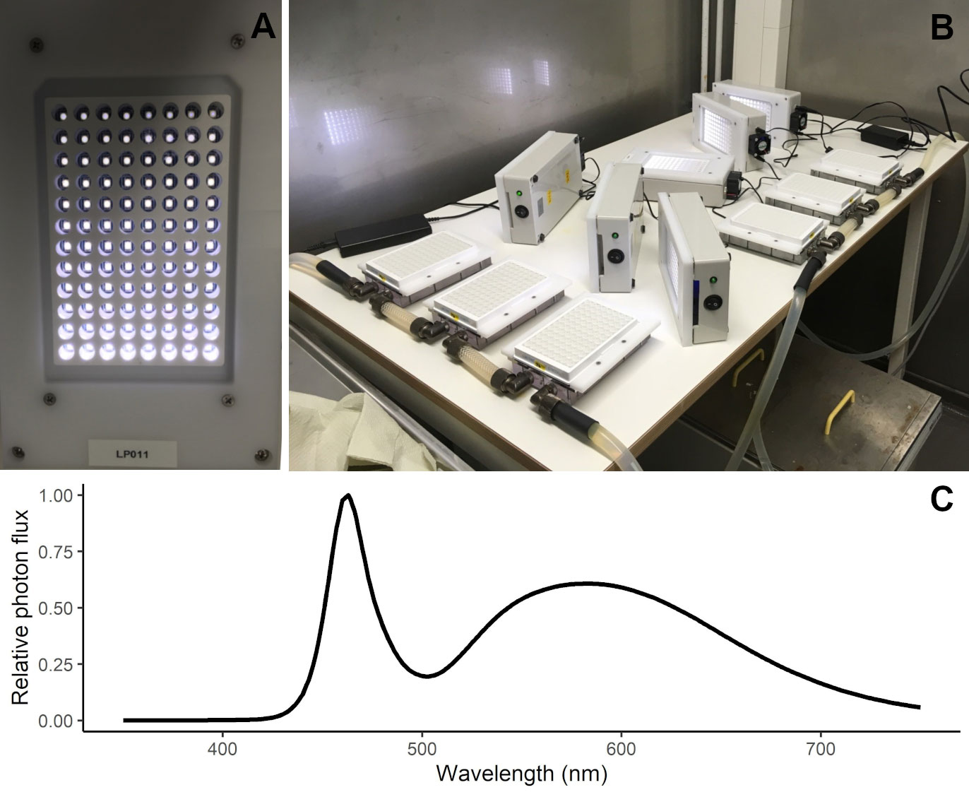
Figure 1 High-throughput well-plate setup used in the experiments. Detail on the LED plate for illuminating individual wells (A) and experiment setup showing the 96-well plates positioned on the temperature-controlled cooling plates with LED panels to the side, ready to be mounted over the well-plates (B). Measured light spectrum (as relative photon flux) in the LED panels used in the experiment (C).

Three Baltic Sea spring dinoflagellates were selected from the FINMARI Culture Collection/Syke Marine Research Laboratory and Tvärminne Zoological Station (FINMARI CC): Apocalathium malmogiense (G. Sjöstedt) Craveiro, Daugbjerg, Moestrup & Calado (strain code SHTV-1, collected in Tvärminne Storfjärden, western Gulf of Finland, in 2002 by A. Kremp), Gymnodinium corollarium A.M. Sundström, Kremp & Daugbjerg (strain code GCTV03, collected at station BY15, in the Baltic Proper, in 2007 by A. Kremp) and Heterocapsa arctica subsp. frigida Rintala & G. Hällfors (strain code HATV-1401, collected in Tvärminne Storfjärden, western Gulf of Finland, in 2014 by P. Hakanen). In the culture collection, these strains are maintained at a 14:10 light:dark cycle, at 4°C, using f/2 medium (Guillard and Ryther, 1962, but excluding the Si), the base of which is filtered and autoclaved Baltic Sea water with the salinity of approximately 6 ‰. Prior to the experiments, the selected strains were pre-acclimated to the used salinities (for 4-12 weeks) and temperatures (for 2-4 weeks). To avoid potential biases associated to dilution of dissolved compounds in the sea water, the f/2 medium with different salinities used in the pre-acclimation and in the experiments was based on artificial sea water and made by diluting sea salt (Tropic Marin, Germany) in Milli-Q water.

Once a culture was pre-acclimated and growing in the different conditions, the cells were inspected using a FlowCam (Fluid Imaging Technologies) equipped with a colour camera, a flow cell FC100 and 10x objective. Images were collected with an auto-image mode and single healthy cells were manually sorted using the Visual Spreadsheet software (Fluid Imaging Technologies). Individual cell volumes were obtained using the area-based diameter algorithm from the Visual Spreadsheet software. To start the experiments, each well was filled with 300 µl of f/2 medium of the appropriate salinity and inoculated with 10-30 µl of the pre-acclimated culture. The amount of inoculum varied according to the density of the stock culture which was determined just before the inoculation by assessing the cell densities and chlorophyll a in vivo fluorescence and aiming at a reading of 130-250 fluorescence units. Chlorophyll a fluorescence (ex./em.: 440/680 nm) of the medium and the test unit immediately after the inoculation was checked using a fluorescence spectrometer (Cary Eclipse, Agilent), equipped with a plate reader accessory, and using the following parameter settings: excitation 440 nm, excitation slit 5 nm, emissions 680 nm, emission slit 5 nm and high voltage (800 V) setting of the photomultiplier. Thereafter, growth in each well was evaluated from chlorophyll a in vivo fluorescence time series, which was measured daily in the same way as described above. A blank plate was filled with f/2 medium and measured daily in the same way as the experimental plates to monitor the background fluorescence of the medium. The daily background medium fluorescence was calculated as the average of the 96 wells each day and this value was subtracted from fluorescence data of that day prior growth rates calculations. To avoid evaporation and contamination between wells, all the plates were covered with an optical clear film, which was exchanged for a new one every time the plates were taken out for reading. For deciding on which type of film to use, we first ran a pilot using a gas-tight (ultra-clear polyester sealing adhesive film for qPCR (VWR)) and a non-gas-tight cover (the non-adhesive cover back film of the sealing qPCR film) to cover 96 well-plates and monitor growth of our study organisms. No difference in light (spectrum nor intensity) was observed between the cover types, which were then evaluated regarding the chlorophyll a in vivo fluorescence growth and evaporation for 20 days at 4 °C. While no difference was observed between cover types for G. corollarium growth, growth of A. malmogiense and H. arctica subsp. frigida were slower in plates covered with the gas-tight membranes in comparison to non-gas tight. Thus, although we first intended to use the sealing qPCR film, we opted for using its non-adhesive protective back film instead. Each set of experiments was carried out with one strain at a time, due to the limited amount of available experimental platforms. The experiments lasted between 11 days (for A. malmogiense and G. corollarium) and 21 days (for H. arctica subsp. frigida). In some cases, treatments reached readings over 500 fluorescence units earlier than others and were discontinued to ensure that the readings were still within the linear dynamic range of the instrument and that the fluorescence readings were directly proportional to the chlorophyll a concentration.

2.2 Statistical analysis

Effects of temperature and salinity on the cell sizes of the three dinoflagellates were tested with cell volume estimates obtained from the FlowCam by the end of the pre-acclimation. For that, a linear model was employed for each taxon, using the cell volumes as response variable and temperature, salinity, and the interaction between them (temperature×salinity) as independent variables. Cell volumes were log-transformed prior to analysis due to their scale-dependent variability. Analysis was done in R version 4.1.0 (R Core Team, 2021). The significance levels for all the analyses were 0.05. All plots were drawn in R using the “ggplot2” package (Wickham, 2016).

Daily fluorescence time series were plotted to follow the growth of each culture under the different experimental conditions and growth rates were determined only from the exponential growth phase. Although the cultures were pre-acclimated to temperature and salinity, this was not done for the light intensities. Thus, in the first days of the incubations (lag growth phase) variations in the chlorophyll a fluorescence were under the effect of light acclimation and were not proportional to the biomass, as the cellular pigmentation changed to match an optimum in a given light level. The exponential growth phase was differentiated from lag and stationary growth phases by assessing differences in the slope values of the fluorescence increase over time. For this, a regression model was estimated using piecewise linear relationships for the detection of breakpoints (Muggeo, 2003). The estimated breakpoints were considered to mark the change in the growth phase for each treatment in each experiment. The fitting of regression models with segmented relationships and break-point estimation was carried in R, using the package “segmented” (Muggeo, 2008). The exponential growth phase was considered to start on the first day after the (first) break point and to finish either by the end of the experiment or at the second breakpoint (that was interpreted to mark the start of the stationary phase), when this was detected. When no breakpoints were detected or not significant, the fluorescence time series were individually checked to determine the beginning of the exponential phase. Growth rates for each well were calculated as in Equation 1 (Levasseur et al., 1993):

$\begin{array}{ll}\mu =(\ln F_f-\ln F_0)/t& \text{Equation 1}\end{array}$

Where $F_f$ is the chlorophyll a fluorescence by the end of the exponential growth phase, $F_0$ is the chlorophyll a fluorescence at the beginning of the exponential growth phase, and $t$ is the number of days between $F_0$ and $F_f$.

The resulting growth patterns were used to estimate the photo-physiological traits of each taxon by fitting a growth-irradiance curve at different temperature and salinity levels. At first, we aimed to evaluate the light limitation by fitting the growth-irradiance curve with a simpler two-parameter model (MacIntyre et al., 2002; Equation 2). However, as some of the tested organisms displayed a negative effect of high light intensities on growth, we also fitted a three-parameter model to evaluate light limitation and photoinhibition (Eilers and Peeters, 1988; Equation 3). Note that negative growth rates were excluded prior to model fitting.

$\begin{array}{ll}\mu (E)={\mu }_{max}\times e^{\frac{-E}{K_E}}& \text{Equation 2}\end{array}$

$\begin{array}{ll}\mu (E)= \frac{{\mu }_{max}\times E}{\frac{{\mu }_{max}}{\alpha \times I_{op}^2}\times E^2+(1-2\times \frac{{\mu }_{max}}{\alpha \times I_{op}})\times E+\frac{{\mu }_{max}}{\alpha }}& \text{Equation 3}\end{array}$

In Equation 2, the observed growth ($\mu$) over the different light intensities ($E$) is parameterized as the maximum growth rate at optimal light intensities (${\mu }_{max}$) and the light-saturation parameter ($K_E$). In Equation 3 the observed growth ($\mu$) over the different light intensities ($E$) is described by the maximum growth rate at optimal light intensities (${\mu }_{max}$), the irradiance in which growth rate is maximum ($I_{op}$) and the initial slope of the growth-irradiance curve ($\alpha$) of a given species. The parameters for both models were estimated with nonlinear least squares in R using the package “nlme” (Pinheiro et al., 2021). Only parameters with significant estimates are reported in our results.

2.3 Long-term monitoring data

Alg@line phytoplankton monitoring data (n = 3396) collected across the Baltic Sea (Travemünde-Helsinki) between 1993-2011 using ships-of-opportunity (Finnjet 1993-1997; Finnpartner 1998-2006; Finnmaid 2007-2011) was utilized to put the experiment findings into an environmental context. The sampling focused on spring, summer and autumn, with fewer samplings during the winter months December, January and February. The commercial ferry route across the Baltic Sea reflects multiple environmental gradients, including temperature and salinity. The FerryBox system pumps water collected at ∼ 5 m depth that is representative of the entire productive layer (Rantajärvi et al., 1998). The water is distributed at a flow rate of 2-4 L min^-1 through different sensors, including a temperature and conductivity sensor from which temperature and salinity were obtained. Along the transect, discrete water samples were collected using an automated sampler (ISCO) and stored in it in refrigerated and unlit conditions until they were brought ashore for analysis. In 1993-1995 sampling was scheduled to take place at specific times, from 1996 onward samples were taken at specific longitudinal positions. Throughout the study period the methods used were essentially the same although the models and makes of some apparatus varied. Phytoplankton samples were preserved with acid Lugol’s solution (Willén, 1962) and settled following the Utermöhl method (Utermöhl, 1958). In brief, 50 ml of sample was settled for ≥ 24 hours and the whole chamber bottom was examined under a 10x objective, and two bottom diameters were examined using the 40x objective. The phytoplankton species composition was determined with the accuracy permitted by inverted light microscopy of acid Lugol’s preserved samples. The semi-quantitative phytoplankton abundance assessment followed the HELCOM guidelines (HELCOM, 2011) and the occurrence of each taxon in a sample was classified in five ranks: 1 = very sparse (only one or a few cells in the analysed area), 2 = sparse (slightly more cells in the analysed area), 3 = scattered (several cells in many fields of view), 4 = abundant (several cells in most fields of view), and 5 = dominant (many cells in every field of view). For a more detailed description see Hällfors (2013).

Since Heterocapsa arctica subsp. frigida was formally described only in 2010 (Rintala et al., 2010) this taxon was recorded in the long-term monitoring data mainly at genus level. However, the main person analysing the phytoplankton species composition, Seija Hällfors, who also participated in the species description in 2010, was aware of the distinct morphology of H. arctica subsp. frigida long before this monitoring began (cf. Hällfors, 2013, and references therein). The overwhelming majority of the records of Heterocapsa sp. in the data are H. arctica subsp. frigida, and based on notes covering the years 1993-2005 (i.e. the data utilized in the study by Rintala et al., 2010), some other Heterocapsa sp. observations were excluded for that period. Between 2006-2011, such notes were not evaluated, and while there is a chance that a few other Heterocapsa observations are included, we are confident that most of the genus-level records are in fact H. arctica subsp. frigida. Apocalathium malmogiense and Gymnodinium corollarium are part of a species complex, the Apocalathium complex (also termed Scrippsiella/Biecheleria/Gymnodinium complex (Sundström et al., 2010), and Scrippsiella complex (Jaanus, 2011)). Because A. malmogiense and G. corollarium cannot reliably be differentiated in acid Lugol’s fixed samples, and furthermore, because in the early years of the monitoring data these species were both identified as Scrippsiella hangoei, we chose to sum the occurrences of all species belonging to this species complex and treat it collectively as the Apocalathium complex. To recalculate the abundance ranks when taxonomical units were joined within a sample, we used the highest observed rank among the merged taxonomical units, as the maximum number of merged taxonomical units was three (Hällfors, 2013). The occurrences of H. arctica subsp. frigida and the Apocalathium complex in different temperatures and salinities over the years were visualised by kernel density estimates, with peaks denoting where more observations were recorded.

3 Results

3.1 Effects of temperature and salinity on cell volume

Potential effects of temperature (3, 6, and 9°C) and salinity (4-9 ‰) on the cell volume of the three dinoflagellates was evaluated by the end of the pre-acclimation period. At salinity 9 ‰, cell volumes could not be determined for A. malmogiense (all temperatures) and for G. corollarium (at 3°C) due to technical issues. On average, A. malmogiense was larger (mean ± sd = 6451 ± 1947 µm³, n = 19360) than G. corollarium (mean ± sd = 3586 ± 1245 µm³, n = 26027). As expected, both above mentioned species were markedly larger than H. arctica subsp. frigida (mean ± sd = 1062 ± 391 µm³, n = 7289). Cell volumes were significantly affected by temperature for all three dinoflagellates (p< 0.001) and by salinity (p< 0.001 for A. malmogiense and H. arctica subsp. frigida; p = 0.004 for G. corollarium). The interaction between temperature and salinity was only significant for G. corollarium (p< 0.01). Cell volumes were similar across temperature for A. malmogiense, but cells were larger at 3°C and smaller at 9°C (Figure 2). G. corollarium and H. arctica subsp. frigida were smaller at 3°C (with slightly larger cells at 6°C) and larger at 9°C, with the increase in cell sizes at 9°C being pronounced for H. arctica subsp. frigida (Figure 2). The cell volume of A. malmogiense did not seem to be affected by variations in salinity, while H. arctica subsp. frigida cell volume was consistent across salinities at 6°C, but a tendency towards larger cells was observed for the other temperatures at salinity 9 ‰ (Figure 2). At 3 and 6°C, G. corollarium cells were smaller at intermediate salinities (5-7 ‰) and increased towards both low and high salinities, however at 9°C average cell decreased with increasing salinity (Figure 2).

FIGURE 2

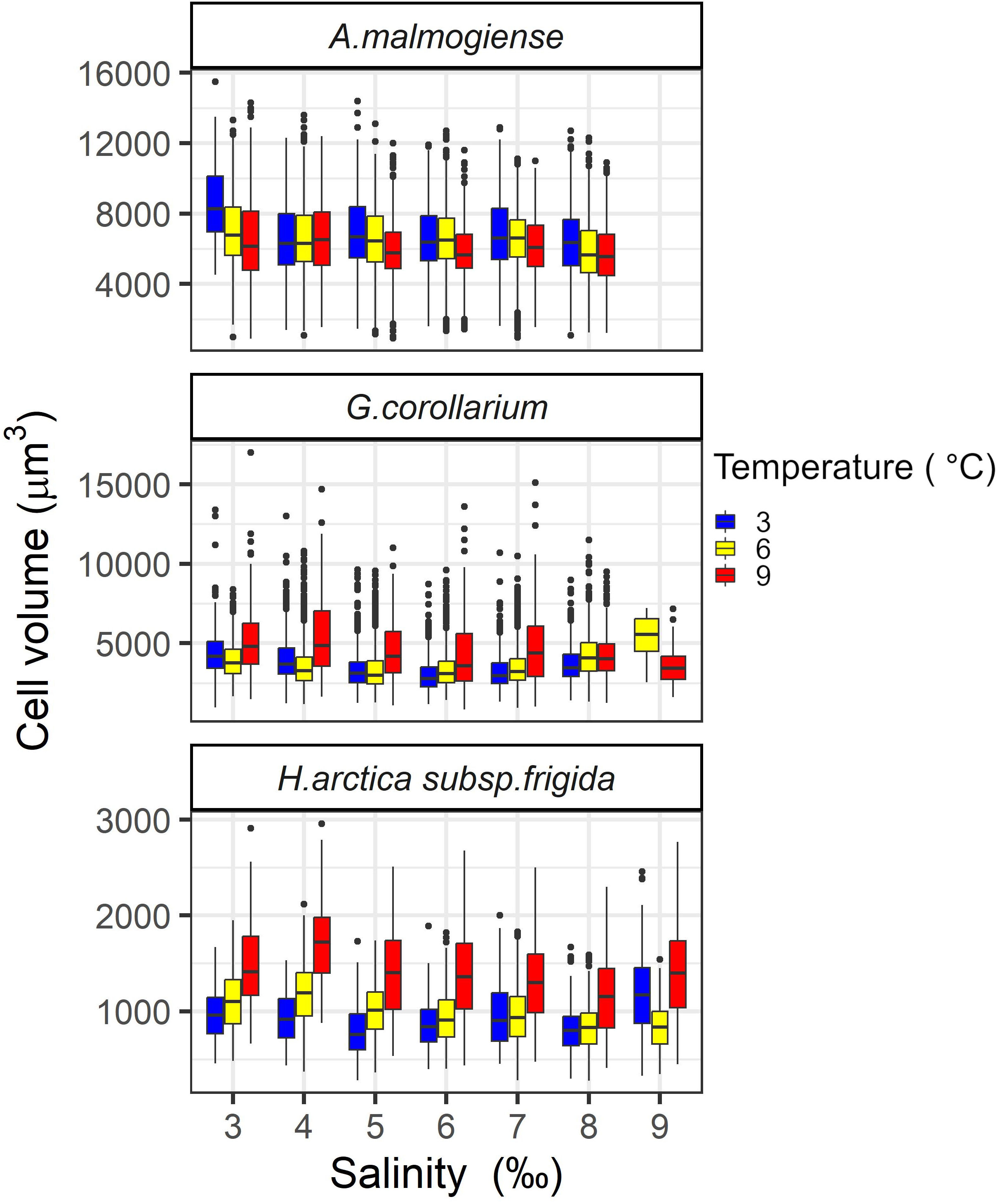
Figure 2 Variations in cell volumes of Apocalathium malmogiense, Gymnodinium corollarium, and Heterocapsa arctica subsp. frigida after the pre-acclimation to the salinities and temperatures used in the experiment.

3.2 Effects of temperature, salinity and light intensity on growth rates

The three dinoflagellates grew differently in the treatments. A. malmogiense was the only species to grow in all temperatures (3, 6, and 9°C), salinities (4-9 ‰) and light intensities (Figure 3). Variability among the replicates of A. malmogiense increased at 9°C, more pronouncedly at lower salinities and higher light intensities (Figure 3). G. corollarium growth was detected in all salinities at 3 and 6°C, while at 9°C consistent growth among the replicates could only be detected in salinity 5 ‰ (Figure 4). G. corollarium did not grow in the highest light intensity (550 µmol photon m² s^-1) and at 350 µmol photon m² s^-1 growth was only detected in salinities 5-8 ‰ at 3°C and 5-9 ‰ at 6°C (Figure 4). G. corollarium replicates exhibited the lowest variability among the three dinoflagellates, being quite consistent in the treatments where growth was detected (Figure 4). Growth in H. arctica subsp. frigida was observed for all salinities (4-9 ‰) in temperatures of 3 and 6°C, however at 9°C this species only grew in 6 and 7 ‰ (Figure 5). Although growth was detected at 9°C and 6 ‰, the replicates were not consistent resulting in large variation in these treatments (Figure 5). Similarly to G. corollarium, H. arctica subsp. frigida did not grow at the highest light intensity (Figure 5).

FIGURE 3

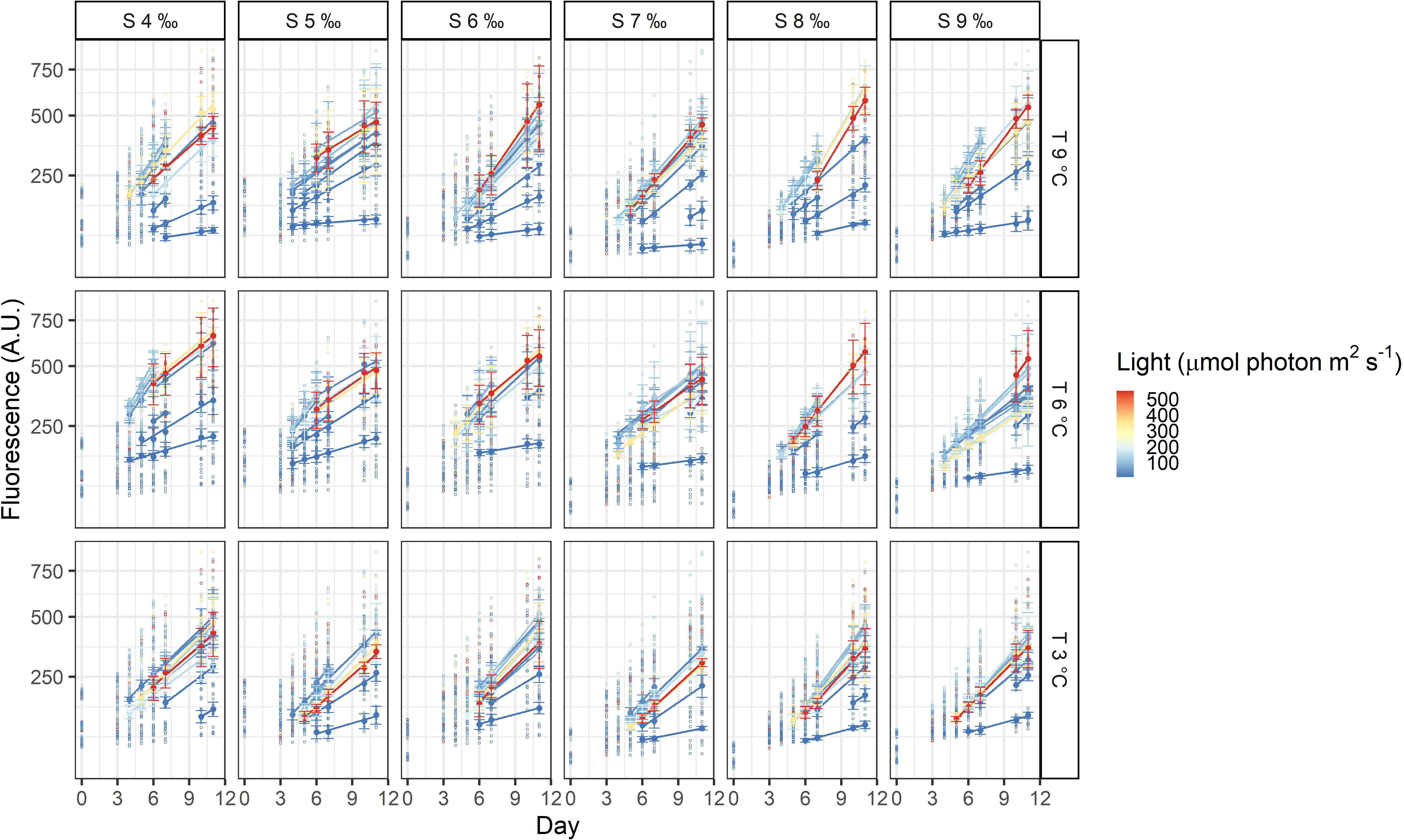
Figure 3 Fluorescence time series of Apocalathium malmogiense. Each circle is the observed fluorescence of each well in each day. Daily means and standard deviations of the observations used to calculate the growth rates are depicted as full points with the error bars. The lines are linear regressions, included only for visualization purposes.

FIGURE 4

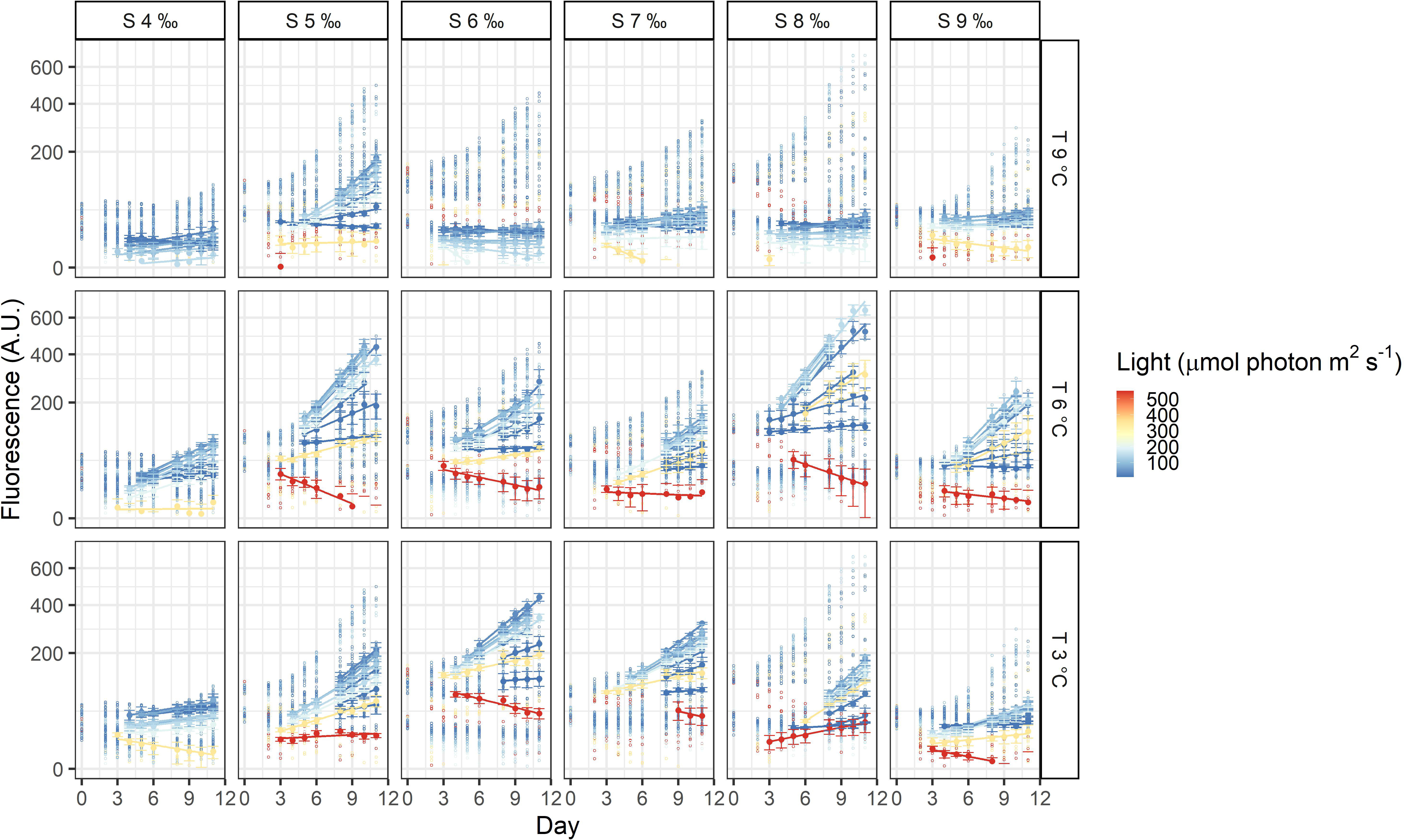
Figure 4 Fluorescence time series of Gymnodinium corollarium. Each circle is the observed fluorescence of each well in each day. Daily means and standard deviations of the observations used to calculate the growth rates are depicted as full points with the error bars. The lines are linear regressions, included only for visualization purposes.

FIGURE 5

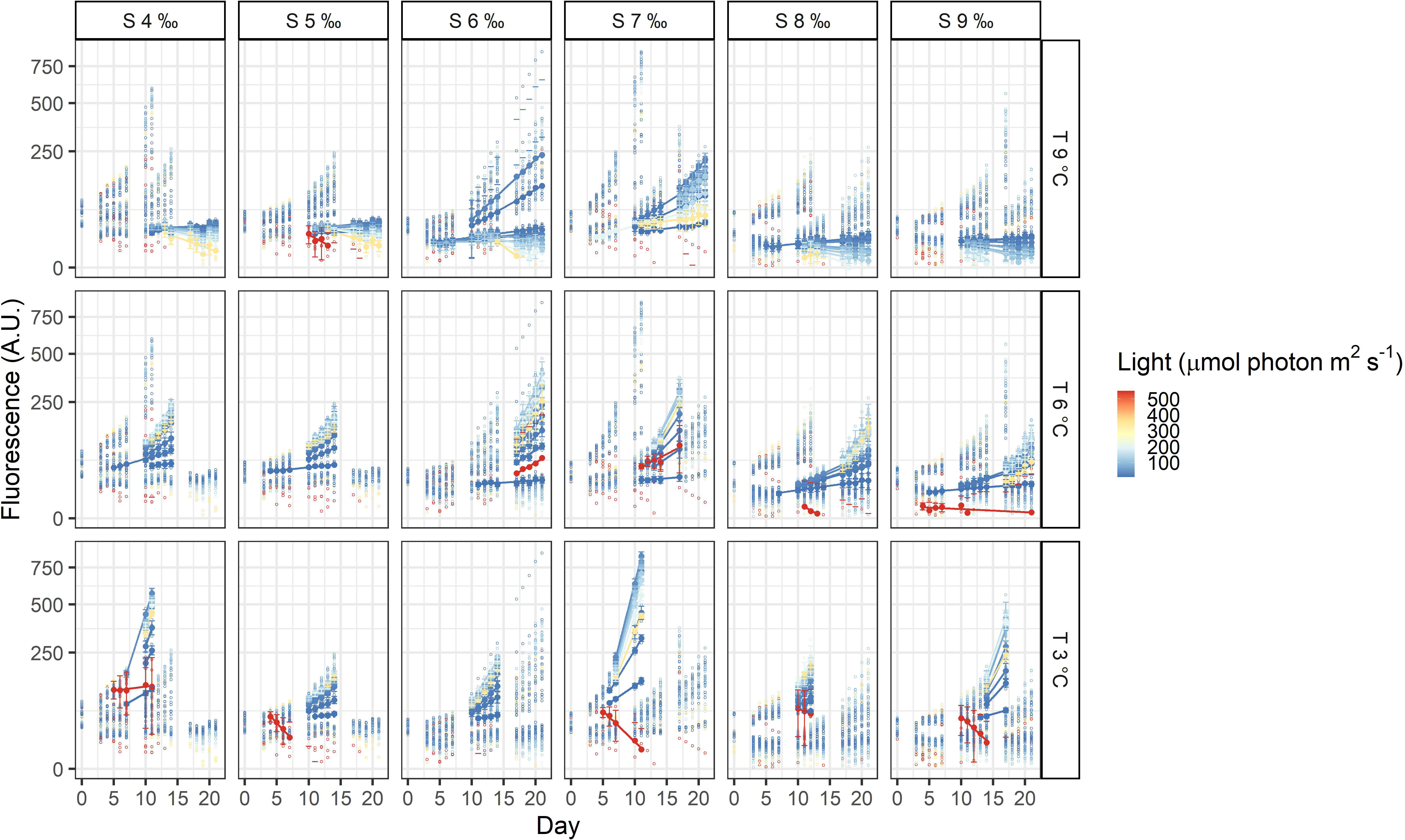
Figure 5 Fluorescence time series of Heterocapsa arctica subsp. frigida. Each circle is the observed fluorescence of each well in each day. Daily means and standard deviations of the observations used to calculate the growth rates are depicted as full points with the error bars. The lines are linear regressions, included only for visualization purposes.

None of the three dinoflagellates grew in all treatments and the highest observed growth rates across all experiments were 0.38, 0.32, and 0.25 d^-1 for A. malmogiense, G. corollarium and H. arctica subsp. frigida, respectively (Figure 6). Growth rates for A. malmogiense were higher (>0.25 d^-1) at 3°C (all salinities), while at 6 and 9°C such high growth rates were restricted to salinities ≥ 6 ‰ (Figure 6). High growth rates for G. corollarium and H. arctica subsp. frigida (≥0.20 d^-1) were mostly observed at 6°C, although for the latter growth rates were higher in salinities ≥6 ‰ (Figure 6). Light intensities also affected the dinoflagellates growth, influencing the fitting of the two models. A. malmogiense showed a weaker tendency to photoinhibition, which was only featured in few treatments (salinities 6, 8, and 9 ‰ at 3°C and salinity 9 ‰ at 6°C) (Figure 6). In contrast, G. corollarium and H. arctica subsp. frigida were more sensitive to higher light intensities, showing photoinhibition for light intensities > 150 and 175-200 µmol photon m² s^-1, respectively. Curiously, H. arctica subsp. frigida was not photoinhibited at 6°C in salinities 8-9 ‰ (Figure 6).

FIGURE 6

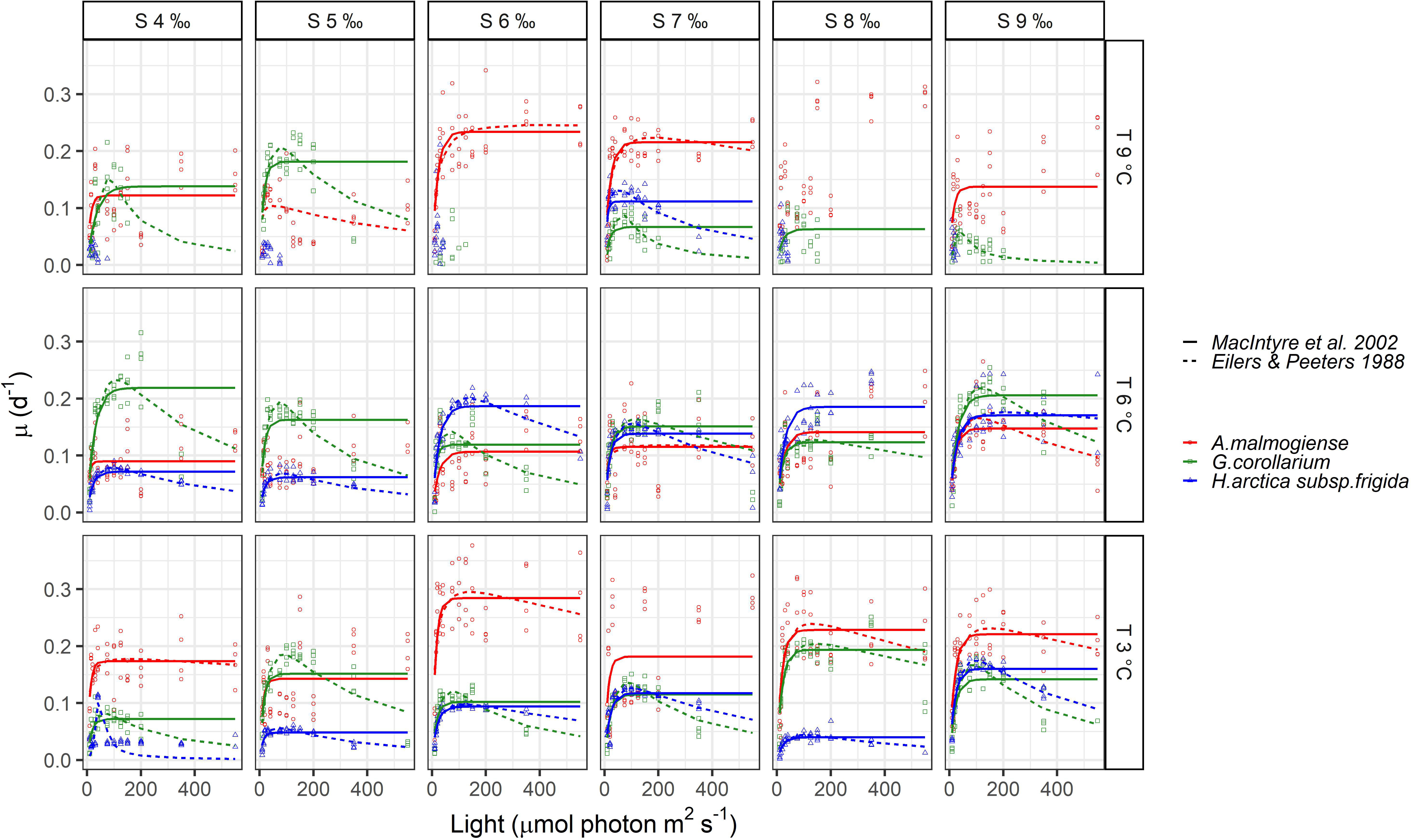
Figure 6 Observed growth rates for Apocalathium malmogiense, Gymnodinium corollarium, and Heterocapsa arctica subsp. frigida. The curves represent the fitted growth-intensity models (MacIntyre et al., 2002 and Eilers & Peeters, 1988) in different temperatures and salinities.

The two growth-irradiance models indicated similar maximum growth rates at optimal light intensities (µ_max) and saturation intensities for the three dinoflagellates (Figures 6, 7A, C). Overall, estimated µ_max were lower than the observed growth rates (µ) but showed a similar variation pattern over the temperature and salinity gradients (Figures 6, 7A, C). The µ_max estimates ranged between 0.09-0.30 d^-1 for A. malmogiense (highest values found at 3°C and 6 ‰), 0.06-0.23 d^-1 for G. corollarium (highest µ_max at 6°C and 4 ‰), and 0.04-0.20 d^-1 for H. arctica subsp. frigida (highest µ_max recorded at 6°C and 6 ‰) (Figures 7A, C). The light saturation of the growth-irradiance curve (K_E) ranged between 7.17-23.89, 12.03-32.39 and 7.67-25.60 µmol photon m² s^-1 for A. malmogiense, G. corollarium and H. arctica subsp. frigida, respectively. Although differences were observed among the dinoflagellates, K_E tended to be higher at 3 and 6°C and salinities ≥6 ‰ for all three tested taxa (Figure 7B). For the three-parameter model, besides µ_max, two other parameters were described, I_op and α. I_op ranged between 51.78-425.41, 40.21-147.11, and 46.61-227.31 µmol photon m² s^-1 for A. malmogiense, G. corollarium, and H. arctica subsp. frigida respectively. I_op were higher at 3-6°C and salinity >6 ‰ for G. corollarium, and for H. arctica subsp. frigida the values were higher at 6°C and salinity 9 ‰ (Figure 7D). For A. malmogiense the highest I_op was observed at 9°C and 6 ‰, although the number of estimates for this species was limited using the three-parameter model (Figure 7D). A. malmogiense presented the highest α values (0.007-0.032 µmol photon^-1 m² s d^-1), with lower α estimates found for H. arctica subsp. frigida (0.0005-0.012 µmol photon^-1 m² s d^-1) and G. corollarium (0.001-0.012 m² µmol photon^-1 m² s d^-1). α was higher at 3°C and salinity ≤ 6 ‰ for A. malmogiense, while for G. corollarium consistent high values were observed at 6 °C independent on the salinity and for H. arctica subsp. frigida α values were more sensitive to salinity than temperature, with higher values estimated for salinities ≥ 6 ‰ (Figure 7E). The overall relationships between the estimated parameters of each model distinguish A. malmogiense from G. corollarium and H. arctica subsp. frigida for the 3-parameter model (Figures 8A-C), but the difference between dinoflagellates is less clear for the 2-parameter model (Figure 8D).

FIGURE 7

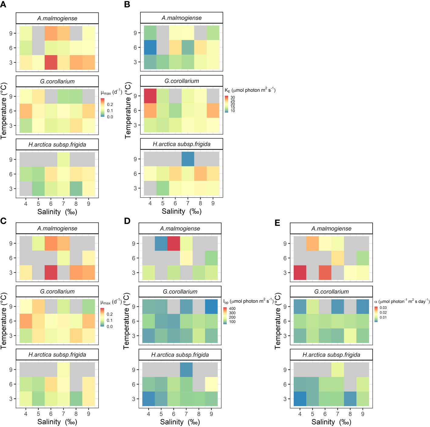
Figure 7 Photo-physiological traits estimated for Apocalathium malmogiense, Gymnodinium corollarium, and Heterocapsa arctica subsp. frigida at different temperatures and salinities. Parameters estimated using MacIntyre et al. (2002) two-parameter (A, B) or Eilers & Peeters (1988) three-parameter models (C–E). Missing and non-significant parameters are depicted in gray.

FIGURE 8

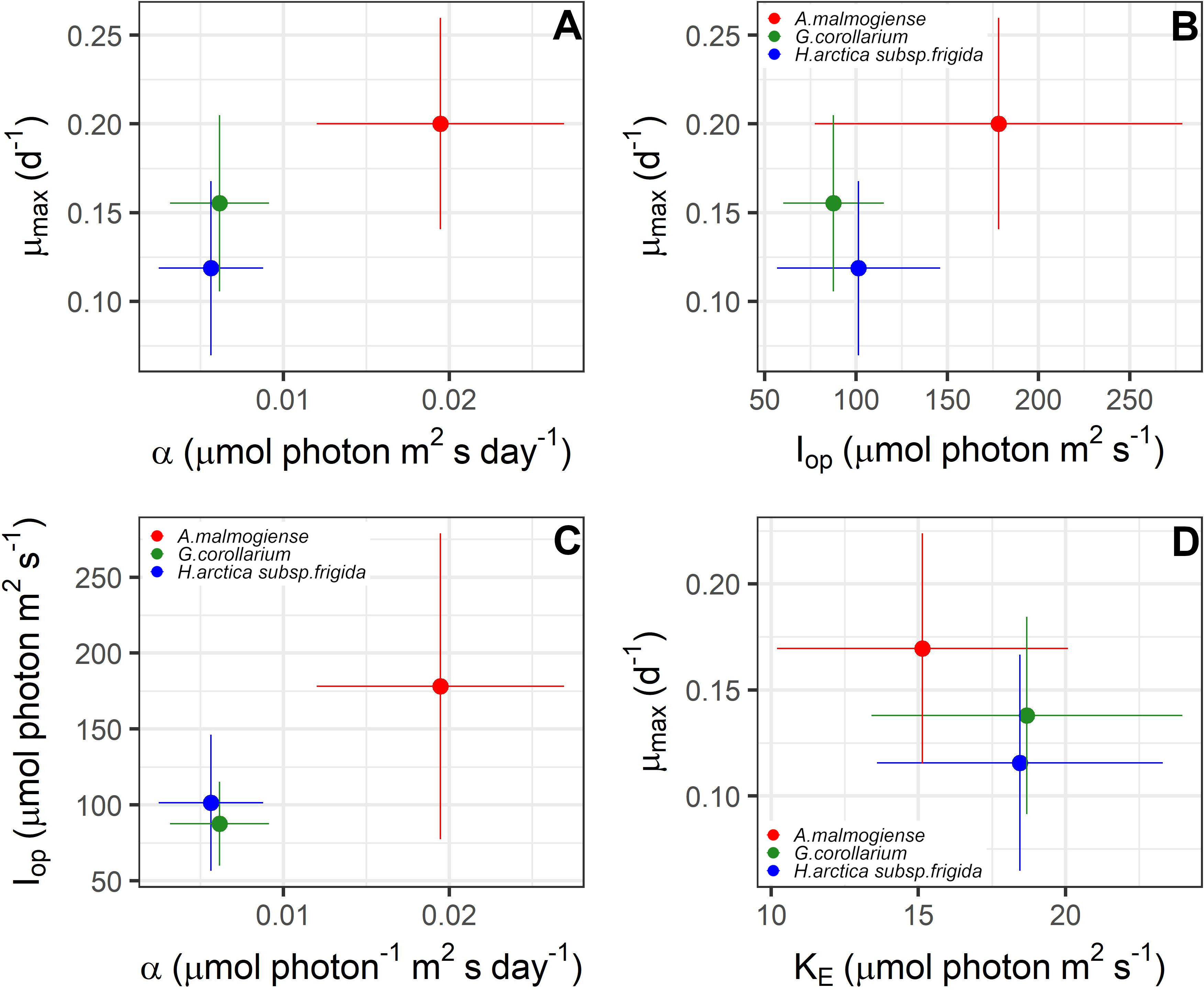
Figure 8 Relationships between photo-physiological traits estimated for Apocalathium malmogiense, Gymnodinium corollarium, and Heterocapsa arctica subsp. frigida. The points depict the averages and the bars the standard deviations found in all the experiments. (A–C) are the parameters estimated using Eilers & Peeters (1988) 3-parameter model; (D) depicts relationship between the two-parameter estimated with MacIntyre et al. (2002) model.

3.3 Occurrence in the Baltic Sea phytoplankton community

Of the 3396 Alg@line monitoring samples collected in 1993-2011, the Apocalathium complex and/or H. arctica subsp. frigida occurred in a total of 1157 samples and more frequently in the northern than southern part of the transect (Figure 9A). The Apocalathium complex was observed in all the months between February to November, although the number of records from July – November is low (less than 15 occurrences for the entire period). H. arctica subsp. frigida was observed between February – June and August – November, however it was usually observed in March, April and May, with scarce occurrence (<10 observations) in other months. Both the Apocalathium complex and H. arctica subsp. frigida were observed most frequently and with higher abundances in April and May. Overall, the long-term data demonstrated that the Apocalathium complex and H. arctica subsp. frigida are usually found in natural samples in temperatures<10°C and salinities 4-10 ‰ (Figures 9B, C), matching the temperature and salinity gradients used in this study.

FIGURE 9

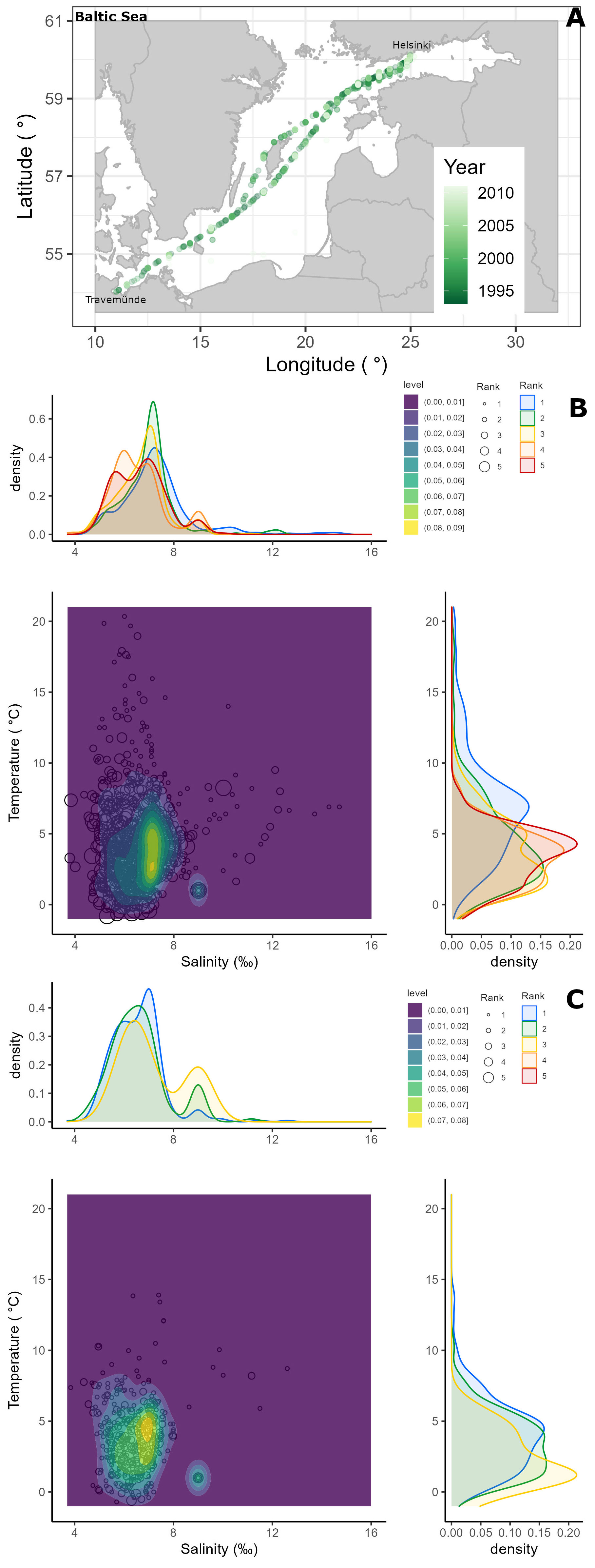
Figure 9 Semi-quantitative phytoplankton data (as abundance ranks) from samples collected in 1993-2011 onboard ships-of-opportunity transversing the Baltic Sea (A), depicting the occurrence of the Apocalathium complex (B) and Heterocapsa arctica subsp. frigida (C) over environmental temperature and salinity gradients.

Both the Apocalathium complex and H. arctica subsp. frigida seem to prefer similar temperature (2-5°C) and salinity (5-7 ‰) ranges, although the occurrence of H. arctica subsp. frigida was more constrained than that of the Apocalathium complex (Figures 9B, C). Abundant and dominant occurrences (ranks 4 and 5) of the Apocalathium complex seem to have a bi-modal distribution for both salinity (peaks at 5 ‰ with highest kernel density estimate ~0.45, and 7 ‰ with highest kernel density estimate 0.4) and temperature (peaks at 4-5°C with highest kernel density estimate ~0.2, and a shoulder at 2.5°C with kernel density estimate 0.12-0.15) (Figure 9B). H. arctica subsp. frigida most frequently occurred at salinities 6-7 ‰ (kernel density estimate 0.35-0.45) and at 0.5°C (kernel density estimate >0.2), although a shoulder (kernel density estimate 0.1) can be observed at around 5°C (Figure 9C).

4 Discussion

Baltic Sea spring dinoflagellates have similar niches regarding their adaptation to cold water and capacity to sustain growth under low nutrient conditions (Kremp et al., 2008; Spilling and Markager, 2008). It has been shown that the cyst formation strategies and seeding conditions from the sediments are essential for the success of certain dinoflagellates species during spring and are susceptible to climate change (Jaanus et al., 2006; Kremp et al., 2008; Spilling et al., 2018). Yet, those factors operate over longer time scales while physiological responses occur at much shorter time scales, providing a contemporary insight into the population dynamics (Harris, 1980), although those remain largely underexplored. We showed that each one of the three tested vernal dinoflagellates have their own niches and preferences regarding photo-acquisition traits. Additionally, temperature and salinity affect the cell volume and response to light availability differently in the three dinoflagellates. Below we present methodological considerations and discuss the implications of our findings for the understanding of the Baltic Sea spring bloom dynamics in face of climate change.

4.1 The high-throughput well-plate setup for phytoplankton trait studies

The high-throughput well-plate setup used in the experiment allows for controlling the light intensity in each well independently and each well-plate to be under temperature controlled conditions, facilitating the conduction of multiple irradiance (Chen et al., 2012; Thrane et al., 2016) and temperature (Thrane et al., 2017) experiments simultaneously. Such experiments would consume much more time and resources if conducted in larger experimental units. This kind of experimental platform has been successfully used to investigate other ecological applications, such as nutrient stoichiometry, organic carbon transformations and screening of optimal growth conditions (Volpe et al., 2021).

Volpe et al. (2021) listed common problems associated with the use of a high-throughput well-plate setup for assessing growth response on microalgae: the temperature variation across the plate associated with different light intensities, evaporation losses and the potential effects of carbon limitation and pH variations on the algae growth. Unlike the setup used in other experiments, our well-plates were illuminated from above and the bottom of the plate was directly in contact with a cooling plate to reduce temperature fluctuations. Additionally, the illumination plate was equipped with a fan to dissipate the heat generated by the LEDs, an improvement also suggested by Volpe et al. (2021). In our experiments we minimized the potential carbon limitation by not using gas-tight membranes. Pilot results indicated potential carbon limitation for A. malmogiense and H. arctica subsp. frigida, since they showed a tendency to slower growth in plates covered with the gas-tight membranes in comparison to non-gas tight ones, while this was not so strongly manifested in G. corollarium (data not shown). It is important to highlight that no difference in the light intensity nor quality was observed between the cover types. During the pilot experiments no significant evaporation loss was observed in the well-plates, regardless of the light intensity, likely because the experiments were carried out at low temperatures.

For the purposes of this study, and taking the precautions explained above, the high-throughput well-plate experimental setup proved to perform well. It should however be noted that some species might not be suitable for testing in the well-plate setup. For example, cultured strains of the chain forming Peridiniella catenata, another common spring dinoflagellate in the Baltic Sea, appear to require more space (larger volumes of medium) for growth in culture. We could not include Biecheleria baltica (which is also part of the Apocalathium complex) in this study, because it failed to grow in the well-plates. As this species does not seem to require larger volumes for its growth, this could result from growing the dinoflagellates in media based on artificial sea water rather than filtered sea water, since some phytoplankton might require certain components, such as organic compounds, not present in artificial mixtures (Berges et al., 2001). We chose to use artificial sea water to account for any potential effects associated with using different salinities, which would require either different dilutions or sea water from different sources, increasing the potential random effects. Future improvements for the design might include testing other growth medium types and/or the addition of soil extract that seems to benefit some organisms. Thus, we recommend testing the growth of a target species in different setups (e.g., culture media, different cover membranes, well-plate suitability) prior to full scale experiments. We also stress that although numerous experiments can be carried out simultaneously in the well-plate setup, the small volume of each well (~300 µl) limits the variables and methods that can be employed to evaluate the experimental responses. Despite the clear suitability of chlorophyll a fluorescence for this setup, the method also has limitations due to relatively narrow linear range of fluorescence measurements from white well-plates (as the ones used in this study), and acclimation effects need to be considered, especially when a light gradient is used (as presented in Material and Methods section).

4.2 Growth rates of vernal Baltic Sea dinoflagellates

Growth rates have been previously reported in the literature for A. malmogiense and G. corollarium, but no such information was found for H. arctica subsp. frigida. Scrippsiella hangoei (syn. A. malmogiense) was reported to grow equally well in 0-30 ‰ and to tolerate temperatures > 6°C (Kremp et al., 2005). A. malmogiense growth varied from 0.18 to 0.33 d^-1 in temperatures 0-11°C, but growth was negatively affected for temperatures >11°C, with no growth detected above 14 °C (Hinners et al., 2017). G. corollarium was reported to grow well in 1.5-12 ‰ salinities, with optimal growth rates at 9 ‰ (0.51 divisions per day or µ = 0.35 d^-1) and in 2-6°C temperatures, with optimal growth rates at 4°C (0.47 divisions per day or µ = 0.33 d^-1) (Sundström et al., 2009). Thus, the growth rates obtained in our experiments were comparable with previous studies for both A. malmogiense (maximum µ = 0.38 d^-1) and G. corollarium (maximum µ = 0.32 d^-1). Additionally, considering that relatively slow growth rates characterize Baltic Sea spring dinoflagellates, especially in comparison to diatoms, which form the other dominant phytoplankton group during springtime in the Baltic Sea (Kremp et al., 2008; Spilling and Markager, 2008), our growth rates estimates appear to be realistic.

4.3 Considerations on selected growth-irradiance models

Multiple Growth-Irradiance models for phytoplankton have been used (e.g. Eilers & Peeters, 1988; MacIntyre et al., 2002; Edwards et al., 2015; Lacour et al., 2017), but it is not unequivocally clear which of these models best describes the photo-physiology traits. While our primarily choice was the model by MacIntyre et al. (2002) based on its simplicity and robustness, the model is unable to reproduce photoinhibition, as observed in G. corollarium and H. arctica subsp. frigida. To be able to capture the photoinhibition component (I_op), which was a relevant aspect for some of the tested organisms, it was clear that another model was needed. In fact, we tested fitting two additional models, a two-parameter model by Steele (1962), which is defined by µ_max and I_op (data not shown), and the three-parameter model by Eilers & Peeters (1988). Despite the simplicity of the Steele model, it consistently yielded higher estimates for both µ_max and I_op than the same parameters estimated by the Eilers and Peeters model. Additionally, the µ_max estimated with both the MacIntyre et al. and Eilers & Peeters models, were similar (for H. arctica subsp. frigida) or better (for A. malmogiense) related to the observed growth rates than the Steele model, but this was not the case for G. corollarium, in which the Eilers & Peeter and Steele models had similar fitting and parameter estimate (data not shown). From those observations we can conclude that although a simpler formulation might be the first target, the model choice should ultimately take into consideration the degree of photoinhibition experienced by the targeted organism. Finally, we chose to present results from fitting both the MacIntyre et al. and Eilers & Peeters models, in order to be as comprehensive as possible, but at the same time provide comparable parameter estimates for the three tested dinoflagellates and more comparability with earlier studies as these models have been used e.g. by Schwaderer et al. (2011); Edwards et al. (2015), and Lacour et al. (2017).

4.4 Vernal Baltic Sea dinoflagellates - from traits to niches

Unicellular, rather nondescript, about 20-30 µm dinoflagellates, known as the Apocalathium complex, occur throughout the springtime in the Baltic Sea and occasionally dominate the phytoplankton biomass (Lignell et al., 1993; Larsen et al., 1995; Jaanus et al., 2006). Despite their similar gross morphology (as seen using conventional monitoring methods, i.e. in light microscopical analysis of acid Lugol’s preserved samples), morphological, ultrastructural and molecular evidence sustain the classification of these dinoflagellates into three distinct species (Apocalathium malmogiense, Biecheleria baltica and Gymnodinium corollarium), each with slightly different temperature and salinity preferences (Kremp et al., 2005; Sundström et al., 2009; Sundström et al., 2010). It has been shown that this complex is dominated by Biecheleria baltica (northern Baltic Sea) and G. corollarium (central Baltic Sea), with cyst records indicating a small contribution of A. malmogiense (Spilling et al., 2018 and references therein). This species complex was reported to occur at 4.5-8 ‰ salinities and temperatures of -1.2-13.8°C, with high abundances recorded over a narrower temperature range (-1.2-7.9°C) (Jaanus et al., 2006; Hällfors, 2013). Here we show that for the most abundant occurrences (ranks 4 and 5) the Apocalathium complex displays a bimodal distribution in both salinity and temperature which may indicate slightly different preferences for different species in the complex. This is corroborated by our experiment results, in which A. malmogiense can grow over a broader salinity, temperature and light range than G. corollarium, which seems to be better adapted to temperatures around 6°C and salinities between 5-8 ‰ and is more susceptible to photoinhibition. Higher light acquisition trait values characterize A. malmogiense, which grew faster than G. corollarium at all tested irradiances. However, we evaluated only a limited number of traits and this apparent advantage of A. malmogiense might impose costs to other traits, such as nutrient use efficiency and resistance to predators (Edwards et al., 2015), which could change the competitive ability of the species.

The smaller-sized H. arctica subsp. frigida is a common spring dinoflagellate in the Baltic Sea, usually occurring at< 5°C but being recorded between temperatures -1.2-13.9°C and salinities 4.7-11.5, while occurring more frequently in the lower-salinity northern areas than in the south (Rintala et al., 2010; Hällfors, 2013). H. arctica subsp. frigida does not often reach high abundances, which is demonstrated by the fact that its highest abundance rank in the environmental data is 3; however it can form under-ice blooms (Niemi and Åström, 1987; Hällfors, 2013). In our study, the highest-abundance observations (scattered, rank 3) were more frequent in temperatures<2°C, whereas the occurrence of those over salinity were bimodal. Very sparse and sparse observations (ranks 1-2) mostly occurred at salinities<8 and between 2-5°C, thus our experiment results agree well with the occurrence observed in natural samples. Likely its slower growth rates, associated with a limited niche for light acquisition, influences the capacity of this dinoflagellate to form blooms. The limited niche for light acquisition can result from an adaptation to also living in sea ice (Rintala et al., 2010), and the fact that α responds to both temperature and salinity may also reflect an adaptation to switching between life in sea ice and open water. H. arctica subsp. arctica has been shown to form temporary cysts (Iwataki, 2002), although no information on these (beyond a micrograph; Iwataki, 2002: Plate 1, fig. 3) or the cyst formation conditions were provided. In the H. arctica subsp. frigida original description, no mention of cysts (temporary or resting) is provided (Rintala et al., 2010), however structures resembling temporary cysts were observed in culture but they were not investigated further.

Growth rate and resource acquisition traits partly define the competitive ability of species in a community and these traits will ultimately respond to the expression of multiple physiological characteristics (Litchman and Klausmeier, 2008). When considering steady state growth under nutrient-saturated conditions, variations in the growth-irradiance relationships can be due to: 1) differences in the light-harvesting properties; 2) changes in the photosynthesis quantum requirement; 3) changes in the photosynthesis to respiration ratios; 4) variations in the amount of fixed carbon exudated; and 5) changes in the photosynthetic quotients (Falkowski et al., 1985). We consider that our experimental observations correspond to a steady state growth under nutrient-saturated conditions, as we only analysed the exponential growth phase. Additionally, considering that the phytoplankton growth medium has plenty of macronutrients and the slow exponential growth rates observed for the tested dinoflagellates, we believe that the effects of nutrient limitation in our experiments were negligible.

Light acquisition traits are the manifestation of many underlying cell features (e.g. pigment composition and their cell quotas, metabolism, respiration, photoprotection, ability to capture photon energy and fix carbon) that change in response to changes in the environment, as long as they are within the ranges defined by the cell genotype (Falkowski et al., 1985; Edwards et al., 2015). Thus, temperature variations are likely to affect the light acquisition traits, due to the thermal effects in the cell metabolism that will change the respiration to photosynthesis ratio (Raven and Geider, 1988) and also due to effects of temperature on electron transport rates (Reynolds, 2006). Although temperature variation also affects the enzymes in the photosynthetic apparatus, they are less sensitive to temperature than the cell metabolism (Raven and Geider, 1988; Dewar et al., 1999). However, such effects can be observed over short-term scales (minutes-hours), while over the course of days to weeks (like in this study) a steady state is reached due to the establishment of balanced carbon fluxes (Dewar et al., 1999). Thus, although factors such as the cell volume or cell specific chlorophyll a and carbon content were not measured at the end of the experiment, we believe that our results capture the resulting steady state over gradients. Our observations indicate that the light acquisition traits in the three studied dinoflagellates are affected by both temperature and salinity. Although the thermal effect on metabolism is more pronounced, salinity might also affect the respiration to photosynthesis ratio, due to osmoregulation costs. Additionally, salinity variation might also have a direct effect on photosynthesis, as ionic stress was shown to stimulate cyclic electron flow and inhibited non-cyclic flow in the chlorophyte Dunaliella tertiolecta (Gilmour et al., 1985). Even though such effects have not been demonstrated for dinoflagellates, one could assume that similarly to temperature, combined effects of salinity on cell metabolism and photosynthetic apparatus can ultimately affect growth rates.

Size is usually a good trait predictor influencing important characteristics such as growth and resource acquisition (Litchman and Klausmeier, 2008). Overall, self-shading is reduced in smaller cells and smaller phytoplankton tend to have a higher light absorption efficiency (α) (Kirk, 2010). Metanalysis studies in freshwater and marine environments found that µ_max and α tend to be negatively correlated with cell size, while no significant relationship was found for I_op (Tang, 1996; Schwaderer et al., 2011; Edwards et al., 2015). Our cell volumes showed, as was expected, that H. arctica subsp. frigida is much smaller (mean 1062 µm³) than G. corollarium (mean 3586 µm³) and A. malmogiense (mean 6451 µm³). Thus, based only on cell size, one could expect H. arctica subsp. frigida to have the highest µ_max and α, with A. malmogiense and G. corollarium having similar values. However, we observed the highest µ_max, I_op and α for A. malmogiense, while G. corollarium and H. arctica subsp. frigida showed similar values for these parameters. This exemplifies that when assessing species with a similar niche generic assumptions such as the allometric scaling might not always apply, as those relationships are a generalization and more suitable over a broader context. We note that A. malmogiense and H. arctica subsp. frigida are thecate dinoflagellates and the theca is absent in G. corollarium, differentiating the tested dinoflagellates regarding their cell wall structure. Although light scatter and absorption might be influenced by cell coverage (Witkowski et al., 1998) and affect the light acquisition traits, the effects of cell sizes, pigment amount and cell contents on those traits are likely to be disproportionally larger than the presence or absence of a theca (Smayda, 1997; MacIntyre & Cullen, 2005).

Our results indicate that the cell sizes of G. corollarium and H. arctica subsp. frigida are more sensitive to temperature variations than that of A. malmogiense. Meantime, G. corollarium light acquisition traits seem to be relatively constant over the tested salinity and temperature gradients, while growth under low light is negatively affected by salinity for A. malmogiense. The efficiency of H. arctica subsp. frigida to use absorbed light for growth increases with both salinity and temperature. At salinity 9 ‰, α becomes similar among the three dinoflagellates, although irregular growth and/or lower growth rates indicate signs of stress in these dinoflagellates. In light of the predicted milder winters, with increased water temperature and light availability in the Baltic Sea (Groetsch et al., 2016), our results indicate that changes in the environmental conditions during spring will likely affect the size distribution and the photo-acquisition traits within the spring bloom communities. Such changes can affect both matter and energy flow in the system, by altering the photosynthesis/respiration ratio, exudation of organic carbon and particle degradation and sinking (Falkowski et al., 1985; Lacour et al., 2017).

5 Conclusions

In this study, we showed that although Baltic Sea vernal dinoflagellates occur in similar salinity and temperature ranges, they have their own niches. We presented novel data on H. arctica subsp. frigida, which despite its occurring in low abundances is a ubiquitous component of the Baltic Sea spring bloom. Furthermore, we demonstrate that G. corollarium and A. malmogiense have distinct niches regarding their light acquisition strategies reinforcing the occurrence of different traits among the Apocalathium complex. Although all three tested dinoflagellates are well adapted to low light conditions, an increase in light availability can impact the vernal Baltic Sea dinoflagellate assembly, selecting for species that can tolerate high light (such as A. malmogiense) in contrast to others that are more prone to photoinhibition (such as G. corollarium and H. arctica subsp. frigida). Additionally, the cell volume, growth and light acquisition traits of the three tested dinoflagellates respond differently to small changes in the ranges of temperature and salinity that are found in the Baltic Sea, demonstrating that photo-acquisition traits can also be used to assess climate change effects, especially when considering short-term effects on species competition. Platforms such as the high-throughput well-plate setup used in this study can ease the arduous task of obtaining physiological trait data. Our results illustrate that this kind of information is essential to answer questions related to species capacity to adapt and compete under a changing environment, especially when complemented by long term phytoplankton monitoring data.

Data availability statement

The raw data supporting the conclusions of this article will be made available by the authors, without undue reservation.

Author contributions

LH and JS conceived the experiments. LH and KK performed the experiments with assistance of PY and JS. PY, SK and TT developed the high-throughput well-plate used in the experiments. HH and LH organized the semi-quantitative monitoring data. LH analysed the data and wrote the first manuscript draft. All authors contributed to the article and approved the submitted version.

Funding

This study was funded by the SEASINK project (Academy of Finland, grant # 317297). LH was funded by Academy of Finland (NanOCean, grant # 342223) and KK was supported by Tiina and Antti Herlin Foundation.

Acknowledgments

This study utilized research infrastructure as part of FINMARI (Finnish Marine Research Infrastructure consortium). We thank Lot van Berkel and Johanna Oja for their assistance during the experiments; and the Alg@line team and Seija Hällfors for their contribution to the ship-of-opportunity phytoplankton time series. We are grateful for Tom Andersen and Geir Andersen help for implementing the LED panels. Also, we thank the reviewers for their valuable comments and suggestions, which helped improve the manuscript.

Conflict of interest

The authors declare that the research was conducted in the absence of any commercial or financial relationships that could be construed as a potential conflict of interest.

Publisher’s note

All claims expressed in this article are solely those of the authors and do not necessarily represent those of their affiliated organizations, or those of the publisher, the editors and the reviewers. Any product that may be evaluated in this article, or claim that may be made by its manufacturer, is not guaranteed or endorsed by the publisher.

References

Berges J. A., Franklin D. J., Harrison P. J. (2001). Evolution of an artificial seawater medium: improvements in enriched seawater, artificial water over the last two decades. J. Phycol. 37 (6), 1138–1145. doi: 10.1046/J.1529-8817.2001.01052.X

CrossRef Full Text | Google Scholar

Chen M., Mertiri T., Holland T., Basu A. S. (2012). Optical microplates for high-throughput screening of photosynthesis in lipid-producing algae. Lab. Chip 12 (20), 3870–3874. doi: 10.1039/C2LC40478H

PubMed Abstract | CrossRef Full Text | Google Scholar

Dewar R. C., Medlyn B. E., Mcmurtrie R. E. (1999). Acclimation of the respiration/photosynthesis ratio to temperature: insights from a model. Global Change Biol. 5 (5), 615–622. doi: 10.1046/j.1365-2486.1999.00253.x

CrossRef Full Text | Google Scholar

Edwards K. F., Thomas M. K., Klausmeier C. A., Litchman E. (2015). Light and growth in marine phytoplankton: allometric, taxonomic, and environmental variation. Limnol. Oceanogr. 60 (2), 540–552. doi: 10.1002/LNO.10033/SUPPINFO

CrossRef Full Text | Google Scholar

Eilers P. H., Peeters J. C. H. (1988). A model for the relationship between light intensity and the rate of photosynthesis in phytoplankton. Ecol. Model. 42 (3–4), 199–215. doi: 10.1016/0304-3800(88)90057-9

CrossRef Full Text | Google Scholar

Falkowski P. G., Barber R. T., Smetacek V. (1998). Biogeochemical controls and feedbacks on ocean primary production. Science 281, 200–206. doi: 10.1126/science.281.5374.200

PubMed Abstract | CrossRef Full Text | Google Scholar

Falkowski P. G., Dubinsky Z., Wyman K. (1985). Growth-irradiance relationships in phytoplankton1. Limnol. Oceanogr. 30 (2), 311–321. doi: 10.4319/LO.1985.30.2.0311

CrossRef Full Text | Google Scholar

Gilmour D. J., Hipkins M. F., Webber A. N., Baker N. R., Boney A. D. (1985). The effect of ionic stress on photosynthesis in Dunaliella tertiolecta. Planta 163 (2), 250–256. doi: 10.1007/BF00393515

PubMed Abstract | CrossRef Full Text | Google Scholar

Groetsch P. M. M., Simis S. G. H., Eleveld M. A., Peters S. W. M. (2016). Spring blooms in the Baltic Sea have weakened but lengthened from 2000 to 2014. Biogeosciences 13 (17), 4959–4973. doi: 10.5194/BG-13-4959-2016

CrossRef Full Text | Google Scholar

Guillard R. R., Ryther J. H. (1962). Studies of marine planktonic diatoms. i. cyclotella nana hustedt, and Detonula confervacea (cleve) gran. Can. J. Microbiol. 8, 229–239. doi: 10.1139/M62-029

PubMed Abstract | CrossRef Full Text | Google Scholar

Hällfors H. (2013). Studies on dinoflagellates in the northern Baltic Sea. PhD thesis (Helsinki:University of Helsinki).

Google Scholar

Harris G. P. (1980). Temporal and spatial scales in phytoplankton ecology. mechanisms, methods, models, and management. Can. J. Fisheries Aquat. Sci. 37 (5), 877–900. doi: 10.1139/f80-117

CrossRef Full Text | Google Scholar

HELCOM (2011) Manual for marine monitoring in the COMBINE programme of HELCOM. part c. programme for monitoring of eutrophication and its effects. annex 6: guidelines concerning phytoplankton species composition, abundance and biomass. Available at: http://www.helcom.fi/groups/monas/Combin%0AeManual/AnnexesC/en_GB/annex6/%0A.

Google Scholar

Hinners J., Kremp A., Hense I. (2017). Evolution in temperature-dependent phytoplankton traits revealed from a sediment archive: do reaction norms tell the whole story? Proc. R. Soc. B: Biol. Sci. 284, 20171888. doi: 10.1098/RSPB.2017.1888

CrossRef Full Text | Google Scholar

Hjerne O., Hajdu S., Larsson U., Downing A., Winder M. (2019). Climate driven changes in timing, composition and size of the Baltic Sea phytoplankton spring bloom. Front. Mar. Sci. 6. doi: 10.3389/FMARS.2019.00482/BIBTEX

CrossRef Full Text | Google Scholar

Honkanen M., Müller J. D., Seppälä J., Rehder G., Kielosto S., Ylöstalo P., et al. (2021). The diurnal cycle of pCO₂ in the coastal region of the Baltic Sea. Ocean Sci. 17 (6), 1657–1675. doi: 10.5194/OS-17-1657-2021

CrossRef Full Text | Google Scholar

Ikävalko J., Thomsen H. A. (1997). ‘The Baltic Sea ice biota (March 1994): a study of the protistan community’. Eur. J. Protistol. 33, 229–243. doi: 10.1016/S0932-4739(97)80001-6

CrossRef Full Text | Google Scholar

Iwataki M. (2002). Taxonomic study on the genus heterocapsa (Peridiniales, dinophyceae). PhD thesis (Tokyo:University of Tokyo).

Google Scholar

Jaanus A. (2011). Phytoplankton in Estonian coastal waters – variability, trends and response to environmental pressures. PhD thesis (Tartu:Tartu University).

Google Scholar

Jaanus A., Hajdu S., Kaitala S., Andersson A., Kaljurand K., Ledaine I., et al. (2006). Distribution patterns of isomorphic cold-water dinoflagellates (Scrippsiella/Woloszynskia complex) causing “red tides” in the Baltic Sea. Hydrobiologia 554 (1), 137–146. doi: 10.1007/S10750-005-1014-7

CrossRef Full Text | Google Scholar

Kahru M., Nömmann S. (1990). The phytoplankton spring bloom in the Baltic Sea in 1985, 1986: multitude of spatio-temporal scales. Continental Shelf Res. 10 (4), 329–354. doi: 10.1016/0278-4343(90)90055-Q

CrossRef Full Text | Google Scholar

Kirk John T. O. (2010). Light and photosynthesis in aquatic ecosystems. 3rd edn (Cambridge:Cambridge University Press). doi: 10.1017/CBO9781139168212

CrossRef Full Text | Google Scholar

Klais R., Tamminen T., Kremp A., Spilling K., An B. W., Hajdu S., et al. (2013). Spring phytoplankton communities shaped by interannual weather variability and dispersal limitation: mechanisms of climate change effects on key coastal primary producers. Limnol. Oceanogr. 58 (2), 753–762. doi: 10.4319/LO.2013.58.2.0753

CrossRef Full Text | Google Scholar

Klais R., Tamminen T., Kremp A., Spilling K., Olli K. (2011). Decadal-scale changes of dinoflagellates and diatoms in the anomalous Baltic Sea spring bloom. PloS One 6 (6), e21567. doi: 10.1371/JOURNAL.PONE.0021567

PubMed Abstract | CrossRef Full Text | Google Scholar

Kremp A., Elbrächter M., Schweikert M., Wolny J. L., Gottschling M. (2005). Woloszynskia halophila (Biecheler) comb. nov.: a bloom-forming cold-water dinoflagellate co-occurring with scrippsiella hangoei (Dinophyceae) in the Baltic Sea. J. Phycol. 41 (3), 629–642. doi: 10.1111/J.1529-8817.2005.00070.X

CrossRef Full Text | Google Scholar

Kremp A., Rengefors K., Montresor M. (2009). Species specific encystment patterns in three Baltic cold-water dinoflagellates: the role of multiple cues in resting cyst formation. Limnol. Oceanogr. 54 (4), 1125–1138. doi: 10.4319/LO.2009.54.4.1125

CrossRef Full Text | Google Scholar

Kremp A., Tamminen T., Spilling K. (2008). Dinoflagellate bloom formation in natural assemblages with diatoms: nutrient competition and growth strategies in Baltic spring phytoplankton. Aquat. Microbial. Ecol. 50 (2), 181–196. doi: 10.3354/AME01163

CrossRef Full Text | Google Scholar

Lacour T., Larivière J., Babin M. (2017). Growth, chl a content, photosynthesis, and elemental composition in polar and temperate microalgae. Limnol. Oceanogr. 62, 43–58. doi: 10.1002/lno.10369

CrossRef Full Text | Google Scholar

Larsen J., Kuosa H., Ikävalko J., Kivi K., Hällfors S. (1995). A redescription of Scrippsiella hangoei (Schiller) comb. nov. –a “red tide” dinoflagellate from the northern Baltic. Phycologia 34 (2), 135–144. doi: 10.2216/I0031-8884-34-2-135.1

CrossRef Full Text | Google Scholar

Levasseur M., Thompson P. A., Harrison P. J. (1993). Physiological acclimation of marine phytoplankton to different nitrogen sources. J. Phycol. 29 (5), 587–595. doi: 10.1111/J.0022-3646.1993.00587.X

CrossRef Full Text | Google Scholar

Lignell R., Heiskanen A.-S., Kuosa H., Gundersen K., Kuuppo-Leinikki P., Pajuniemi R., et al. (1993). Fate of a phytoplankton spring bloom: sedimentation and carbon flow in the planktonic food web in the northern Baltic. Mar. Ecol. Prog. Ser. 94, 239–252. doi: 10.3354/meps094239

CrossRef Full Text | Google Scholar

Litchman E., de Tezanos Pinto P., Klausmeier C. A., Thomas M. K., Yoshiyama K. (2010). Linking traits to species diversity and community structure in phytoplankton. Hydrobiologia 653 (1), 15–28. doi: 10.1007/s10750-010-0341-5

CrossRef Full Text | Google Scholar

Litchman E., Klausmeier C. A. (2008). Trait-based community ecology of phytoplankton. Annu. Rev. 39, 615–639. doi: 10.1146/annurev.ecolsys.39.110707.173549

CrossRef Full Text | Google Scholar

MacIntyre H. L., Cullen J. J. (2005). “Using cultures to investigate the physiological ecology of microalgae,” in Algal culturing techniques. Ed. Andersen R. A. (Cambridge:Cambridge: Academic Press), 287–326.

Google Scholar

MacIntyre H. L., Kana T. M., Anning T., Geider R. J. (2002). Photoacclimation of photosynthesis irradiance response curves and photosynthetic pigments in microalgae and cyanobacteria. J. Phycol. 38 (1), 17–38. doi: 10.1046/J.1529-8817.2002.00094.X

CrossRef Full Text | Google Scholar

Muggeo V. M. R. (2003). Estimating regression models with unknown break-points. Stat Med. 22, 3055–3071. doi: 10.1002/sim.1545

PubMed Abstract | CrossRef Full Text | Google Scholar

Muggeo V. M. R. (2008) Segmented: an r package to fit regression models with broken-line relationships. Available at: https://cran.r-project.org/doc/Rnews/.

Google Scholar

Niemi Å., Åström A.-M. (1987). Ecology of phytoplankton in the tvärminne area, SW coast of finland. IV. environmental conditions, chlorophyll a and phytoplankton in winter and spring 1984 at tvärminne storfjärd. Annales Botanici Fennici 24 (4), 333–352.

Google Scholar

Pinheiro J., Bates D., DebRoy S., Sarkar D., Core Team R. (2021) Nlme: linear and nonlinear mixed effects models. Available at: https://cran.r-project.org/package=nlme%3E.

Google Scholar

Rantajärvi E., Olsonen R., Hällfors S., Leppänen J.-M., Raateoja M. (1998). Effect of sampling frequency on detection of natural variability in phytoplankton: unattended high-frequency measurements on board ferries in the Baltic Sea. ICES J. Mar. Sci. 55 (4), 697–704. doi: 10.1006/JMSC.1998.0384

CrossRef Full Text | Google Scholar

Raven J. A., Geider R. J. (1988). Temperature and algal growth. New Phytol. 110 (4), 441–461. doi: 10.1111/J.1469-8137.1988.TB00282.X

CrossRef Full Text | Google Scholar

R Core Team (2021). R: a language and environment for statistical computing (Vienna, Austria: R Foundation for Statistical Computing). Available at: http://www.r-project.org/.

Google Scholar

Reynolds C. S. (2006). The ecology of phytoplankton (Cambridge: Cambridge University Press). doi: 10.1017/CBO9780511542145

CrossRef Full Text | Google Scholar

Rintala J.-M., Hällfors H., Hällfors S., Hällfors G., Majaneva M., Blomster J. (2010). Heterocapsa arctica Subsp. frigida subsp. nov. (Peridiniales, dinophyceae)–description of a new dinoflagellate and its occurrence in the Baltic Sea. J. Phycol. 46 (4), 751–762. doi: 10.1111/J.1529-8817.2010.00868.X

CrossRef Full Text | Google Scholar

Schwaderer A. S., Yoshiyama K., de Tezanos Pinto P., Swenson N. G., Klausmeier C. A., Litchman E. (2011). Eco-evolutionary differences in light utilization traits and distributions of freshwater phytoplankton. Limnol. Oceanogr. 56 (2), 589–598. doi: 10.4319/LO.2011.56.2.0589

CrossRef Full Text | Google Scholar

Smayda T. J. (1997). Harmful algal blooms: their ecophysiology and general relevance to phytoplankton blooms in the sea. Limnol. Oceanogr. 42, 1137–1153. doi: 10.4319/lo.1997.42.5_part_2.1137

CrossRef Full Text | Google Scholar

Spilling K. (2007). Dense sub-ice bloom of dinoflagellates in the Baltic Sea, potentially limited by high pH. J. Plankton Res. 29 (10), 895–901. doi: 10.1093/plankt/fbm067

CrossRef Full Text | Google Scholar

Spilling K., Kremp A., Klais R., Olli K., Tamminen T. (2014). Spring bloom community change modifies carbon pathways and C:N:P: chl a stoichiometry of coastal material fluxes. Biogeosciences 11 (24), 7275–7289. doi: 10.5194/BG-11-7275-2014

CrossRef Full Text | Google Scholar

Spilling K., Markager S. (2008). Ecophysiological growth characteristics and modeling of the onset of the spring bloom in the Baltic Sea. J. Mar. Syst. 73 (3–4), 323–337. doi: 10.1016/J.JMARSYS.2006.10.012

CrossRef Full Text | Google Scholar

Spilling K., Olli K., Lehtoranta J., Kremp A., Tedesco L., Tamelander T., et al. (2018). Shifting diatom-dinoflagellate dominance during spring bloom in the Baltic Sea and its potential effects on biogeochemical cycling. Front. Mar. Sci. 5. doi: 10.3389/FMARS.2018.00327/BIBTEX

CrossRef Full Text | Google Scholar

Steele J. H. (1962). Environmental control of photosynthesis in the sea. Limnol. Oceanogr. 7, 137–150. doi: 10.4319/lo.1962.7.2.0137

CrossRef Full Text | Google Scholar

Stipa T. (2004). The vernal bloom in heterogeneous convection: a numerical study of Baltic restratification. J. Mar. Syst. 44 (1–2), 19–30. doi: 10.1016/J.JMARSYS.2003.08.006

CrossRef Full Text | Google Scholar

Sundström A. M., Kremp A., Daugbjerg N., Moestrup Ø., Ellegaard M., Hansen R., et al. (2009). Gymnodinium corollarium Sp. nov. (Dinophyceae) – a new cold water dinoflagellate responsible for cyst sedimentation events in the Baltic Sea. J. Phycol. 45 (4), 938–952. doi: 10.1111/J.1529-8817.2009.00712.X

PubMed Abstract | CrossRef Full Text | Google Scholar

Sundström A. M., Kremp A., Tammilehto A., Tuimala J., Larsson U. (2010). Detection of the bloom-forming cold-water dinoflagellate Biecheleria baltica in the Baltic Sea using LSU rRNA probes. Aquat. Microbial. Ecol. 61 (2), 129–140. doi: 10.3354/AME01442

CrossRef Full Text | Google Scholar

Tamelander T., Heiskanen A. S. (2004). Effects of spring bloom phytoplankton dynamics and hydrography on the composition of settling material in the coastal northern Baltic Sea. J. Mar. Syst. 52 (1–4), 217–234. doi: 10.1016/J.JMARSYS.2004.02.001

CrossRef Full Text | Google Scholar

Tang E. P. Y. (1996). Why do dinoflagellates have lower growth rates? J. Phycol. 32 (1), 80–84. doi: 10.1111/J.0022-3646.1996.00080.X

CrossRef Full Text | Google Scholar

Thrane J. E., Hessen D. O., Andersen T. (2016). The impact of irradiance on optimal and cellular nitrogen to phosphorus ratios in phytoplankton. Ecol. Lett. 19 (8), 880–888. doi: 10.1111/ele.12623

PubMed Abstract | CrossRef Full Text | Google Scholar

Thrane J. E., Hessen D. O., Andersen T. (2017). Plasticity in algal stoichiometry: experimental evidence of a temperature-induced shift in optimal supply N:P ratio. Limnol. Oceanogr. 62 (4), 1346–1354. doi: 10.1002/lno.10500

CrossRef Full Text | Google Scholar

Utermöhl H. (1958). Methods of collecting plankton for various purposes are discussed. SIL Commun. 9, 1–38. doi: 10.1080/05384680.1958.11904091.

CrossRef Full Text | Google Scholar

Vahtera E., Conley D. J., Gustafsson B. G., Kuosa H., Pitkänen H., Savchuk O. P., et al. (2007). Internal ecosystem feedbacks enhance nitrogen-fixing cyanobacteria blooms and complicate management in the Baltic Sea. AMBIO: A J. Hum. Environ. 36 (2), 186–194. doi: 10.1579/0044-7447(2007)36

CrossRef Full Text | Google Scholar

Volpe C., Vadstein O., Andersen G., Andersen T. (2021). Nanocosm: a well plate photobioreactor for environmental and biotechnological studies. Lab. Chip 21 (10), 2027–2039. doi: 10.1039/D0LC01250E

PubMed Abstract | CrossRef Full Text | Google Scholar

Wickham H. (2016). ggplot2: elegant graphics for data analysis (New York: Springer-Verlag).

Google Scholar

Willén T. (1962). Studies on the phytoplankton of some lakes connected with or recently isolated from the Baltic. Oikos 13 (2), 199. doi: 10.2307/3565084

CrossRef Full Text | Google Scholar

Witkowski K., Król T., Zielinski A., Kuten E. (1998). A lightscattering matrix for unicellular marine phytoplankton. Limnol. Oceanogr. 43, 859–869. doi: 10.4319/lo.1998.43.5.0859

CrossRef Full Text | Google Scholar