Synoptic-to-intraseasonal atmospheric modulation of phytoplankton biomass in the inner sea of Chiloé, Northwest Patagonia (42.5°-43.5°S, 72.5°-74°W), Chile

1 Introduction

Phytoplankton plays an important role in marine ecosystems, producing almost half of the global primary production in the oceans (Field et al., 1998). Phytoplankton dynamics at global and seasonal scales are relatively well known; at mid-latitudes, blooms are mainly driven by abiotic factors such as solar irradiance, water column stratification, nutrient availability, winds, column stratification (Winder and Cloern, 2010; Demarcq et al., 2012; Sapiano et al., 2012). Yet, the characteristics of their spatio-temporal variability at timescales shorter than seasons, especially in coastal areas, remains a challenging issue for science. Coastal areas, which provide 22-43% of the estimated value of the ecosystem services worldwide (Costanza et al., 1997), support a substantial part of the primary production by phytoplankton blooms (Carstensen et al., 2015). In open coastal areas, phytoplanktonic blooms are driven mainly by episodic upwelling events that transport deep water nutrients into the surface layer, with variable intensities at synoptic timescales [i.e., up to ~10 days (Orlanski, 1975)].

When phytoplankton blooms occur, there is a marked increase in algal biomass in response to the rapid transformation and incorporation of reactive inorganic elements into organic forms that leads to measurable biogeochemical changes. As described by Cloern (1996), these processes include the depletion of inorganic nutrients (N, P, Si), shifts in the isotopic composition of reactive elements (C, N), changes in dissolved oxygen and carbon dioxide removal, production of climatically active gases, changes in the biochemical composition and reactivity of the suspended particulate matter, and synthesis of organic matter required for the reproduction and growth of heterotrophs, including bacteria, zooplankton, and benthic consumer animals. For some phytoplankton species, blooms are simply part of their seasonal or interannual natural variability, whereas for others they occur as episodic events, and thus generalisations concerning their triggering mechanisms are not adequate. Therefore, in the latter cases, blooms are still difficult (or even impossible) to predict (Davidson et al., 2016).

Along eastern boundary upwelling systems at mid-latitudes, the intensification of the equatorward alongshore winds during spring and summer promotes seasonal upwelling (Aguirre et al., 2019). Compared to other marine systems, these systems are dominated by short trophic webs where phytoplankton blooms are among the key base processes. However, monospecific phytoplankton blooms involving toxic algae species might induce harmful effects on other species, including humans (Landsberg, 2002; Young et al., 2020; Neves et al., 2021). These events are denominated Harmful Algal Blooms (HABs) and are of particular scientific and societal interest due to their impacts. HABs produce damage to the aquaculture, tourism, and overall economy of local communities and countries. Globally, three different types of HABs can be distinguished (Hallegraeff, 1992). Considering their monospecific nature, they are differentiated by the involved species. First, blooms that cause harmless discoloration of water, which, however, under exceptional conditions in shallow waters and sheltered bays, can be dense enough to cause indiscriminate death of fish and invertebrates through oxygen depletion. Second, blooms that are not toxic to humans but are harmful to fish and invertebrates by damaging or plugging their gills, physically or chemically. They particularly affect animals in intensive aquaculture systems, which cannot escape from danger. Third, the category which most concerns human society corresponds to those algae species that produce potent toxins that can reach human consumers through the food chain, causing a variety of gastrointestinal and neurological diseases, such as paralytic shellfish poisoning, diarrheal shellfish poisoning, amnesic shellfish poisoning and neurotoxic shellfish poisoning, among others. Due to these well-established and further emerging impacts, HAB monitoring has intensified and suggested an increase in HAB frequency (Hallegraeff et al., 2021). Eutrophication, climatic variability, human introduction of alien harmful species, and aquaculture developments have all been put forward as main drivers of HABs. In Chilean Patagonia, all these factors have been suggested as possible precursors of a positive trend in HAB frequency (Cabello and Godfrey, 2016; Mardones et al., 2017; León-Muñoz et al., 2018; Crawford et al., 2021; Soto et al., 2021). However, due to geographic and hydroclimatic complexity, the mechanisms within different spatio-temporal scales that trigger these exceptional phytoplanktonic blooms remain unclear.

Chilean Patagonia is one of the largest estuarine systems worldwide. In the North, one of its major features is the Inner Sea of Chiloé (ISC), which is 230 km long in the meridional direction and comprises a system of complex topography and bathymetry, encompassing islands, peninsulas, channels, and fjords. It sustains a major biological hotspot, with a pelagic trophic web that spans from phytoplankton to blue whales (Buchan and Quiñones, 2016). In recent decades, salmon and shellfish aquaculture has become a major industry and one of Chile’s main economic activities, concentrating particularly in the ISC and the southern fjords and channels to the South, in the Aysén Administrative District. Different aspects of such ecosystems and their economic activities have been studied in depth (e.g., Buschmann et al., 2009; Iriarte et al., 2010; Anbleyth-Evans et al., 2020). Although historical and ongoing research efforts have strongly contributed to the understanding of physical and biogeochemical processes within the ISC, in situ observations are still scarce and limited to fully characterise the diversity of regional phenomena. The differences in the phytoplankton community structure in the ISC is closely linked to environmental heterogeneity that determines the composition and availability of nutrients, particularly the nitrate/silicate ratio (Martínez et al., 2015). While in high silicate environments the larger fraction (>20 µm) predominates, nitrate-rich environments are dominated by smaller phytoplankton (<11 µm). Studies throughout the ISC have highlighted the influence of freshwater inputs from Patagonian rivers with a pluvio-nival regime on coastal circulation, the stratification of the water column and the spatiotemporal variability of nutrient load to the system, in particularly silicate (e.g., León-Muñoz et al., 2013; Iriarte et al., 2017; Vásquez et al., 2021; Flores et al., 2022). In addition, the connection of the ISC with the outer waters of the Pacific Ocean through the Chacao Channel and Boca del Guafo promotes the intrusion of Sub-Antarctic Waters (SAAW) richer in nitrates and phosphates (Silva and Palma, 2006; Vargas et al., 2011). Seasonally, the largest freshwater inputs occur during winter and spring in the northeastern ISC, when several species of the microphytoplankton size-fraction (>20 μm) is dominated by chain-forming freshwater related diatoms of the genera Skeletonema, Chaetoceros, Thalassiosira and Rhizosolenia (Iriarte et al., 2017). On the other hand, marine species such as Rhizosolenia setigera and Thalassiosira subtilis, and genera Coscinodiscus and Leptocylindrus, dominate during autumn months under low levels of freshwater inputs (Iriarte et al., 2017). On a larger scale, sedimentary records have revealed that both marine and freshwater diatoms are abundant in the ISC, however a decreasing trend in the relative abundance of freshwater diatoms during the 20th century has been linked to decreased precipitation and streamflows. of rivers and the occurrence of global El Niño events (Rebolledo et al., 2011; Rebolledo et al., 2015; Iriarte et al., 2017). Recent evidence has shown that the intensity of spring–summer phytoplankton blooms may vary strongly on inter-annual scales in association with variability in remote signals that promote environmental changes along the ISC associated with the thermal regime and freshwater supply to the system (e.g., PDO, ENSO, SAM; Lara et al., 2016). Regarding harmful algal blooms in ISC, where only a few species have been reported as significant contributors to HABs (Lembeye, 2006), an increase in HAB frequency has been observed in recent years, possibly associated in part with eutrophication processes (Folke et al., 1994; Soto et al., 2021). This has raised a special focus from public institutions and the scientific community to identify the main forcings of HABs and strengthen the predictability of these phenomena.

Although the environmental factors that trigger exceptional phytoplankton blooms in northern Patagonia, including HABs, are not totally understood, atmospheric and oceanic circulation along with solar irradiance and freshwater input have been recognized as primary drivers (e.g., Díaz et al., 2021). These drivers are strongly controlled by synoptic and mesoscale atmospheric forcing [in this paper, “mesoscale” refers to the definition used for atmospheric phenomena within the range of a few hundred kilometers (Orlanski, 1975)]. Therefore, the dynamics of certain phytoplankton blooms might be partly driven by ocean-atmosphere interaction within the synoptic-to-intraseasonal (SY-IS) timescale, which spans from a few days to several weeks. Hence, establishing the link between atmospheric forcing and phytoplankton dynamics might improve the predictability of blooms. Consequently, this task might support risk mitigation actions, benefitting particularly the local ecosystems and human communities. In addition, salient anomalies in the atmospheric circulation, particularly teleconnections linking tropical and mid-latitudes phenomena, occur in the intraseasonal time scale (10-60 days). These might exhibit a certain degree of predictability, providing an opportunity for a potential guidance towards risk management. In this sense, the Madden-Julian Oscillation (MJO) is particularly relevant, as its evolution might be predicted up to ~4 weeks in advance (Lu et al., 2020). The MJO is the leading mode of tropical climate variability, mainly depicted by a large-scale convective centre in the tropical band that progresses eastwards with a characteristic period of 30-90 days (e.g., Zhang, 2005). Despite being rooted in the tropics, through its teleconnections, the MJO might also partly modulate mid-latitude climate variability (e.g., Matsueda and Takaya, 2015; Cavalcanti et al., 2021). For instance, the MJO has been associated with oceanographic features such as coastal trapped waves along the southeastern Pacific coast (Rutllant et al., 2004; Oliver & Thompson, 2010). The MJO is also of particular relevance for atmospheric and oceanographic processes in Patagonia, such as atmospheric heat waves (Jacques-Coper et al., 2015; Jacques-Coper et al., 2016) and intraseasonal variability in water temperature (Ross et al., 2015; Narváez et al., 2019), respectively. The MJO can be monitored and quantified by several indices; one of them is the Real-time Multivariate MJO index (RMM; Wheeler and Hendon, 2004), which measures the location and activity of the convective centre through phase and intensity values, respectively. The tropical band is divided in 8 regions and one phase is assigned to each of them; a certain phase is said to be active if the corresponding intensity of the RMM is above 1. As previously mentioned, the MJO has been found to modulate the frequency of heat waves in southeastern Patagonia and central Chile during austral summer (from December to February) through the influence of migratory anticyclonic systems, which tend to be regionally more frequent during active phases 8, and 6 and 8, respectively (Jacques-Coper et al., 2016; Jacques-Coper et al., 2021). As an indication, the reader invited to recall that the geostrophic balance implies that cyclonic (anticyclonic) systems are associated with clockwise (anti-clockwise) rotation in mid-latitudes of the Southern Hemisphere. Considering that active MJO phases tend to occur in progressive sequence and exhibit some persistence, the active MJO phase 4 was suggested, among a novel mid-latitude index, as a precursor for heat waves in central Chile in the timescale of up to 2 weeks (Jacques-Coper et al., 2021). Interestingly, case studies therein show that certain summer heat waves might propagate southward, reaching Patagonia. Moreover, during this process, anomalies in atmospheric circulation and solar radiation might peak over the ISC. Thus, the question on whether such regional anomalies over ISC and their potential impacts (e.g., phytoplankton blooms) can be associated with the MJO arises naturally. In particular, to our best knowledge, the possible biological response within the ISC to the MJO activity has not been previously studied.

Therefore, in this work we explore the potential effect of SY-IS atmospheric variability on the events of high concentration of phytoplankton biomass, or simply high biomass events (HBEs), in the southern part of ISC (S-ISC; 42.5°-43.5°S, 72.5°-74°W). We focus on the austral summer season (DJF; December 1st to February 28th), during which a relatively higher frequency of migratory anticyclones (Aguirre et al., 2021) and HABs occur in southern Chile (Sandoval et al., 2018). Our work is structured as follows: section 2 introduces the study area, data, and methods used; results are shown in section 3: sub-section 3.1 shows the spatio-temporal evolution of atmospheric and oceanic variables centred on the occurrence of HBEs, with a focus on the regional (ISC) and large scales (South Pacific basin); sub-section 3.2 expands such analysis into the mesoscale, focusing on S-ISC; sub-section 3.3 presents the potential modulation of phytoplankton biomass and HBEs by the MJO; and sub-section 3.4 is devoted to two case studies of HBEs occurring during active MJO. Finally, the discussions and conclusions of our findings are presented in section 4.

2 Study area, data, and methods

The study area encompasses the ISC (41.5°-44.5°S, 72°-75.5°W), in particular its southern part, S-ISC (42.5°-43.5°S, 72.5°-74°W), located in the coastal region of western South America (Figure 1A). S-ISC comprises a relatively semi-enclosed and shallow system with depths less than 300 metres. This system is influenced by oceanic waters (higher salinity and nitrate-richer than the local waters) that enter the ISC from the Southwest through the Boca del Guafo passage, along with freshwater (low salinity, silicate-rich) received from precipitation and discharges from various rivers, such as Puelo, Yelcho, and Palena (app. 670, 360, and 800 m³ s^-1 mean annual flows, respectively). This region, which represents an essential part in the national productive and economic system, has paradoxically suffered from a lack of continuous monitoring and therefore a scarcity of data. Although satellite remote sensing of the sea surface has led to the generation of important datasets related to the state of the sea in recent decades, today there are still limitations that pose restrictions to continuous measurements. The ISC is characterised by high spatial variability in oceanographic conditions as well as a great variety of environments, such as inlets, fjords, channels, straits, and estuaries (Narváez et al., 2019). In fact, previous studies have found contrasting hydrographic conditions between the north and the south sections in the ISC, with the Desertores Islands being the geographical divide (Lara et al., 2016; Vásquez et al., 2021). Due to limited in-situ data and the lack of continuous monitoring, most of the research on phytoplankton variability (comprising different species of microalgae) in the fjords and channels of southern Chile has relied on the use of satellite chlorophyll-a as a proxy (e.g., Lara et al., 2016; Iriarte et al., 2017). Chlorophyll-a (CHLA), a green pigment involved in oxygenic photosynthesis, can be measured in situ and also retrieved from remote sensing techniques such as satellite observations. North of the Desertores Islands, both CHLA estimates correlate poorly, because of the high concentrations of suspended sediments and dissolved organic matter associated with river discharge, which negatively influence the satellite readings (Vásquez et al., 2021). In these optically complex waters (called Case II waters), recent studies suggest the use of satellite fluorescence instead of satellite CHLA (Lara et al., 2017; Vásquez et al., 2021). On the other hand, south of the Desertores Islands, phytoplankton is the main driver of water optical properties (Case I waters); therefore, there is a good agreement between the satellite measurements and the in-situ CHLA (Vásquez et al., 2021). In order to be certain that satellite measurements correspond to a proxy for phytoplankton biomass, we focus on the variability of satellite fluorescence (namely normalized fluorescence line height, hereafter nFLH) in a restricted subregion that encompasses S-ISC (blue rectangle in Figure 1A). The climatological fields showing the mean and standard deviation values for nFLH during DJF confirm indeed a meridional gradient with lower (higher) mean but higher (lower) standard deviation values the south (north) of the Desertores Islands (Figures 1B, C).

FIGURE 1

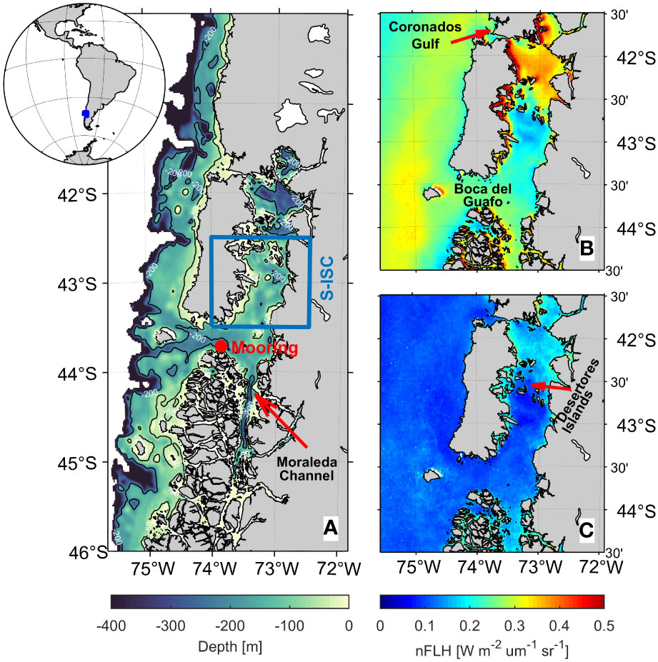
Figure 1 (A) Bathymetry around the Great Chiloé Island, including the Inner Sea of Chiloé (ISC) and the study region, the southern part of ISC (S-ISC, enclosed by a blue square); source: ETOPO1 (https://www.ngdc.noaa.gov/mgg/global/); the inlet at the upper-left corner shows the location of ISC within South America. B, C) Climatological mean and standard deviation fields of normalized fluorescence line height (nFLH) [W m^-2 µm^-1 sr^-1] for summer (DJF 2003-2019), respectively. The main geographical features mentioned in this study are indicated.

In order to comprehensively describe the atmospheric and oceanographic environment that promote HBEs, we analyse several databases at daily resolution (Table 1), including satellite-derived variables and atmospheric fields from ERA5 reanalysis (Hersbach et al., 2020). To incorporate subsurface observations during specific events of high phytoplankton biomass, we use in-situ observations of currents, temperature and salinity from a mooring located at Boca del Guafo (43.7217°S, 73.85481°W; location indicated in Figure 1A), available from November 15, 2018 to January 31, 2019. The mooring consisted in an array of an Acoustic Doppler Current Profile (ADCP) moored face-up at 70m depth, covering up to 15m depth. Temperature was recorded at depths of 20m, 50m, 70m (using a HOBO U24 sensor), 105m (using a miniDOT sensor) and at 140m (using a RBR concerto), salinity (conductivity) was recorded at depths of 20m, 50m, 70m (HOBO U24) and at 140m (RBR).

TABLE 1

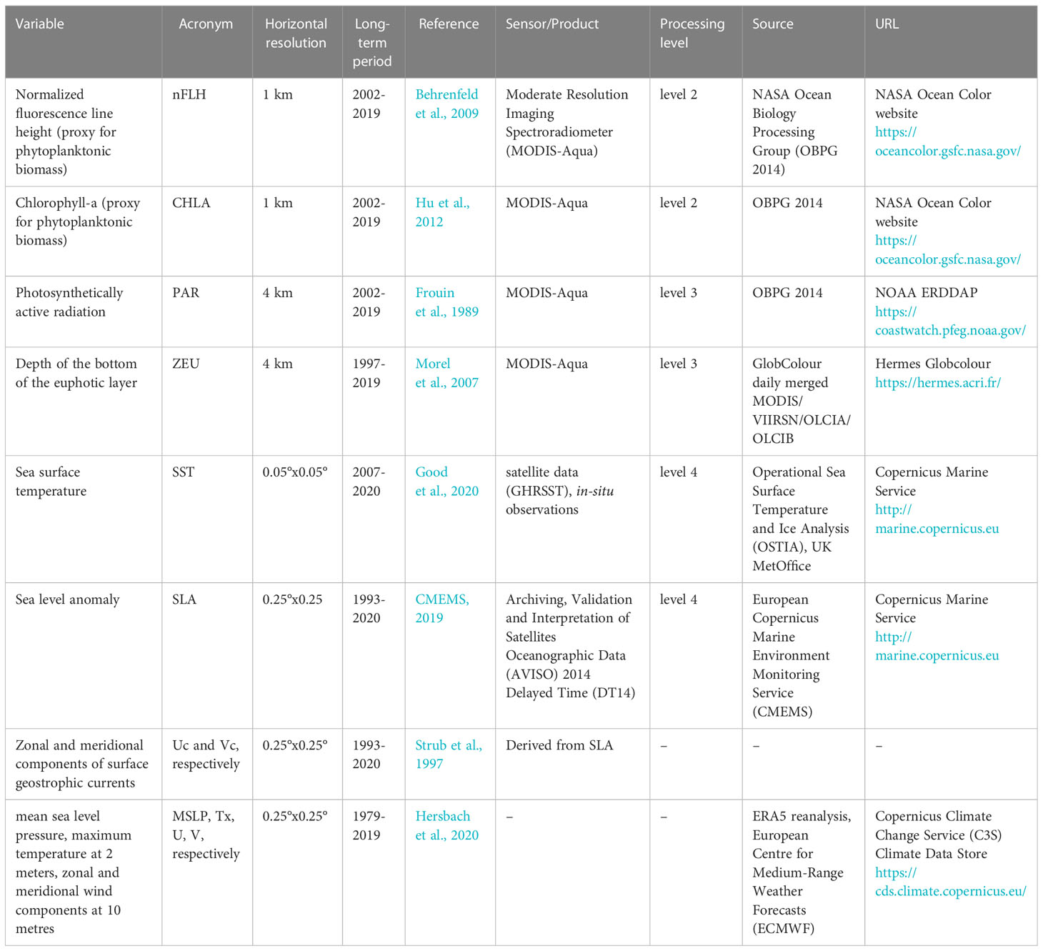
Table 1 Satellite products and reanalysis variables used in this study.

We focus on processes within the timescale spanning from days to weeks. For this analysis, we calculate the SY-IS anomalies following the method proposed by Cerne and Vera (2011) and adapted in subsequent studies (e.g., Jacques-Coper et al., 2021). The corresponding equation reads:

$$\begin{array}{l}\mathit{S}\mathit{Y}\mathit{-}\mathit{I}\mathit{S}\mathit{\_}\mathit{a}\mathit{n}\mathit{o}\mathit{m}\mathit{a}\mathit{l}{\mathit{y}}_{\mathit{i}\mathit{,}\mathit{j}\mathit{,}\mathit{d}\mathit{,}\mathit{y}}\mathit{=}\mathit{r}\mathit{a}\mathit{w}\mathit{\_}\mathit{v}\mathit{a}\mathit{l}\mathit{u}{\mathit{e}}_{\mathit{i}\mathit{,}\mathit{j}\mathit{,}\mathit{d}\mathit{,}\mathit{y}}\mathit{-}\mathit{D}\mathit{J}\mathit{F}\mathit{\_}\mathit{d}\mathit{a}\mathit{i}\mathit{l}\mathit{y}\mathit{\_}\mathit{c}\mathit{l}\mathit{i}\mathit{m}\mathit{a}\mathit{t}\mathit{o}\mathit{l}\mathit{o}\mathit{g}{\mathit{y}}_{\mathit{i}\mathit{,}\mathit{j}\mathit{,}\mathit{d}\mathit{,}\mathit{y}}\\ \mathit{-}(\mathit{D}\mathit{J}\mathit{F}\mathit{\_}\mathit{s}\mathit{e}\mathit{a}\mathit{s}\mathit{o}\mathit{n}\mathit{a}\mathit{l}\mathit{\_}\mathit{m}\mathit{e}\mathit{a}{\mathit{n}}_{\mathit{i}\mathit{,}\mathit{j}\mathit{,}\mathit{y}}\mathit{-}\mathit{D}\mathit{J}\mathit{F}\mathit{\_}\mathit{l}\mathit{o}\mathit{n}\mathit{g}\mathit{\_}\mathit{t}\mathit{e}\mathit{r}\mathit{m}\mathit{\_}\mathit{m}\mathit{e}\mathit{a}{\mathit{n}}_{\mathit{i}\mathit{,}\mathit{j}})\end{array}$$

Specifically, for each gridded variable, the SY-IS anomaly for a certain gridpoint of coordinates (i, j) for a certain day d and year y corresponds to the residual resulting as the difference between the raw value minus the long-term DJF daily climatological mean (which accounts for the expected annual cycle), minus the corresponding DJF departure of the specific DJF season from the DJF long-term mean (a difference which accounts for the inter-annual variability). For computing daily mean climatological values, the long-term period of each dataset was used (Table 1). However, the analysis and results were restricted to the period covered by the nFLH dataset (DJF 2003-2019, where the year corresponds to the JF months). For each variable, the resulting SY-IS anomalies are denoted with a prime (i.e., nFLH’).

Blooms indicate events of extremely high phytoplanktonic biomass. Therefore, they might be identified as extremely high levels in nFLH. Hence, with the aforementioned consideration, we focus on events of high phytoplankton biomass (HBEs), defined as those events for which nFLH surpasses its long-term 95th percentile (nFLH’>p95). In addition, we also explore the conditions leading to low nFLH’ events, i.e., below the 5th percentile (nFLH’<p05); for consistency, they are termed low biomass events (LBEs). In this way, we aim at following a procedure to explore the atmospheric patterns associated with opposite nFLH’ extreme events. Due to nFLH data availability issues (in most cases due to considerable cloud cover), for the calculation of said nFLH’ thresholds, and hence the corresponding extreme events, we only considered those days that exhibited data availability greater than 50% of the gridpoints within S-ISC considering satellite products at 1km (an area equivalent to ~3000 km²). Above such availability level, we consider spatial average values to be representative of the characteristics within the study area. Moreover, to avoid autocorrelation due to averaging consecutive days that fulfil the intensity condition, each event was characterised by the corresponding first day (of a sequence of days) during which the corresponding threshold was surpassed. The characterization of the development of the S-ISC environment and the regional and synoptic conditions around HBEs was achieved through composite analysis of the aforementioned variables. That is, we compute the daily mean anomaly fields (i.e., composites) for the sequence of days centred on day 0, extending from day -7 to day +7. We first focus on the atmospheric forcing, then on the oceanic response, and finally integrate both to interpret their interaction and suggest a possible mechanism promoting HBEs. All in all, the goal of the aforementioned procedure is to describe the main synoptic pattern related to HBEs and the potential ocean-atmospheric coupling it might reveal.

Furthermore, to explore a possible modulation of HBEs by the MJO, we identify all days within our analysis period that exhibit active phases, i.e., intensity of the MJO RMM index above 1, and select the first day of each group of consecutive days. Then, for each phase, we construct mean fields of mean sea level pressure anomaly (MSLP’), a key variable defining weather patterns, and nFLH’, as the main biological response variable in S-ISC. In this way, we investigate the frequency distribution of active MJO phases and construct a MSLP’/nFLH’ composite for each of them. In parallel, all HBEs are classified according to their corresponding MJO condition (phase and intensity) and qualitatively compared against the expected distribution derived from the MJO climatology. In this way, we contrast the composites obtained from the MJO modulation perspective and those obtained by focusing on HBEs. Finally, we select two case studies: January 23rd, 2013, and January 17th, 2019. Both correspond to HBEs of particular interest, as they occurred during active MJO phases and are also related to HABs. We describe them thoroughly, centering our analysis on the main similarities and differences with respect to the previously exposed composites.

3 Results

3.1 Regional and large-scale conditions leading to HBEs

We identify a set of 16 HBEs, the focus of this paper (Table 2), and 18 LBEs (the corresponding figures will be shown in the Supplementary Material). The duration of each HBE is computed as the amount of consecutive days above the corresponding threshold. So defined, these events last for 1.8 days on average. Figure 2 exhibits the 15-day sequence of anomaly composites of MSLP’ and nFLH’ obtained from the 16 HBEs. These are centred on their onset, i.e., on day 0, and span from day -7 to day +7. First, we explore the evolution of these fields at the regional scale around the ISC (Figure 2A). Between days -7 and -4, we observe mostly negative nFLH’ values (i.e., lower-than-normal values, blue shading) in S-ISC. From day -5 on, we observe the characteristic pattern of intensifying migratory anticyclonic anomalies (depicted by the red contours) over the ISC. As will be shown in Figure 4A (upper panel), the mean signal of such anomalies corresponds to high SLP values. Therefore, for simplicity, in the rest of the paper we will refer to the corresponding pattern directly as “anticyclone”, i.e., an anticyclonic regime. Specifically, the NW-SW MSLP’ gradient increases towards day 0, when it reaches its maximum strength. As will be shown below, the eastern flank of this high pressure system induces southerly wind, which reaches S-ISC during this progression. On day -3, the culmination of a coastal low (negative MSLP’ contours) is evident to the north of Chiloé Island. Progressively, positive nFLH’ values (red shading) populate the ISC from day -3 to day 0, when they reach their highest values, exceeding 0.2 W m^-2 µm^-1 sr^-1 within S-ISC. In S-ISC, the positive nFLH’ anomalies decay towards day +5, returning to negative values that persist at least until day +7. Concomitantly, nFLH’ anomalies in open waters comparable to those within S-ISC also decrease along the Pacific coast around the Coronados gulf (41.6°S, 73.9°W). Figure 2B provides a large-scale perspective of the evolution of the same sequence of days. From day -5 to day 0, we observe the intensification of a mid-latitude anticyclone and its meridional MSLP’ gradient over the southern tip of South America. The influence of this anticyclone over the study area persists clearly until day +5. In turn, Supplementary Figure 1 provides similar figures for the LBEs. In that case, we observe that the anticyclone affects the dynamics of the study area for a shorter period (days -3 to 0) and a strong MSLP’ gradient over S-ISC is observed just on day 0, but not before (as for HBEs). In summary, HBEs are associated with a much more persistent and intense migratory anticyclone than LBEs.

TABLE 2

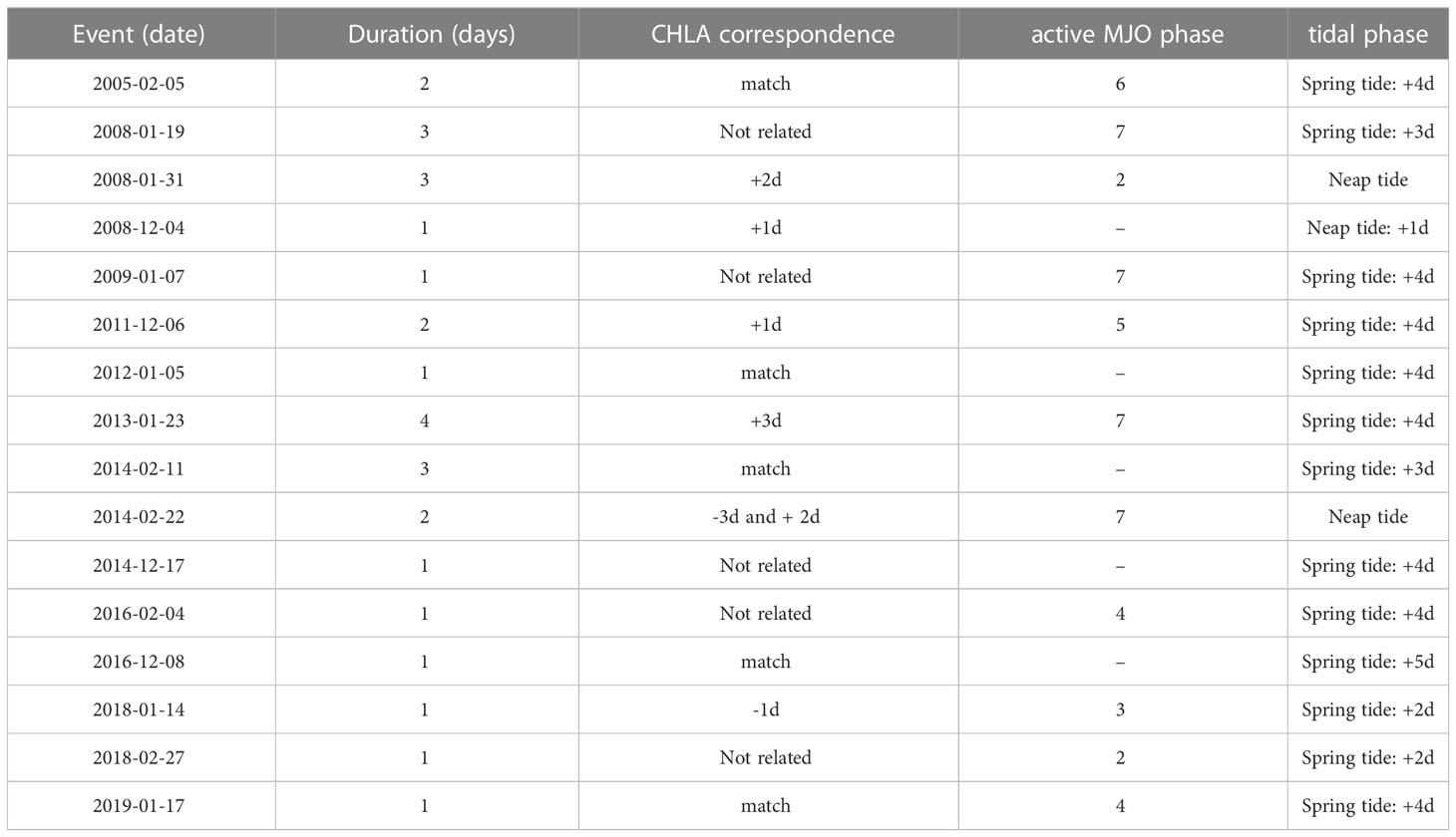
Table 2 Events of high phytoplankton biomass (HBEs): dates of the corresponding day 0, duration (days with spatially averaged nFLH’ above the 95th percentile), correspondence and lag/lead of HBE with respect to CHLA’ events (i.e., days with spatially averaged CHLA’ above its own 95th percentile), corresponding active MJO phase, tidal phase for S-ISC.

FIGURE 2

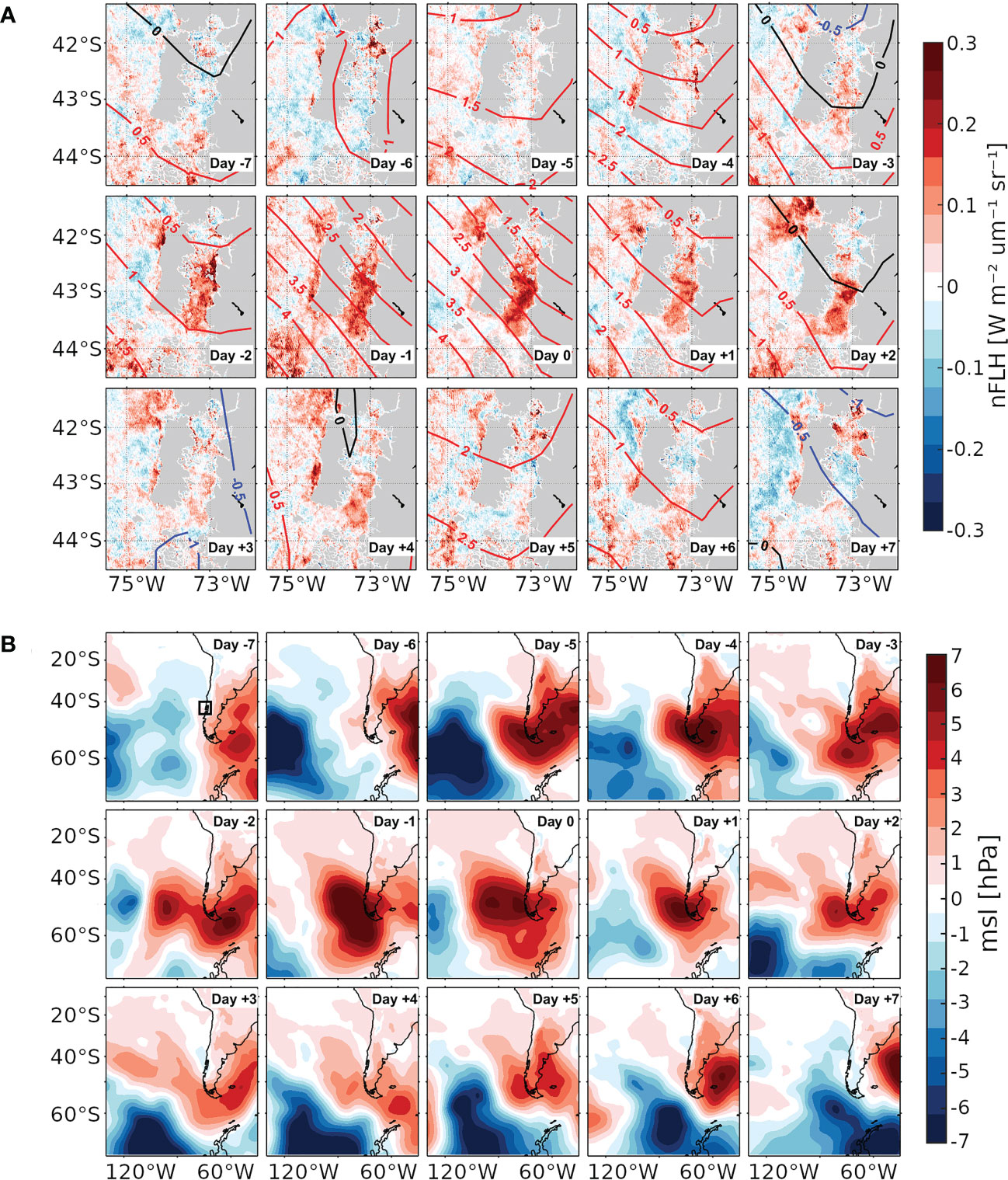
Figure 2 (A) Composites of nFLH’ (shaded, see colour scale [W m^-2 µm^-1 sr^-1]) and MSLP’ (contours every 0.5 hPa, blue/red for negative/positive anomalies) computed for a sequence of days around the 16 HBEs. The sequence is centred on the HBE onset, i.e., on day 0, and spans from day -7 to day +7. (B) MSLP’ fields as in a) (shaded, see colour scale), but extended to a larger-scale covering the southeast Pacific ocean. The box in the upper-left panel indicates the area covered by panel A).

Now, we explore the modulation of the coastal environment by the migratory anticyclone, with a focus on atmospheric and oceanographic processes that occur during HBEs. For this, Figure 3 shows time-latitude Hovmöller diagrams that depict the 15-day mean evolution of the anomalies of key variables over the ISC longitude band (72.5°-74°W), i.e., a broader region than just S-ISC. Again, the diagrams are centred on day 0, which is marked by a dashed vertical white line. In agreement with Figures 2A, 3A exhibits positive nFLH’ values ​​from day -2 to +5, with maximum values around 0.2 W m^-2 µm^-1 sr^-1 over S-ISC on day 0. Recalling the nFLH pattern (absolute values) shown in Figure 1B, a distinction between S-ISC and the northern part of ISC (i.e., north of 42.5°S, N-ISC) is evident. In fact, S-ISC constitutes a region geographically limited to the north by the Desertores Islands and dynamically to the south by the incoming circulation from oceanic waters. The CHLA’ evolution (Figure 3B) shows maximum values around 5 mg m^-3 over S-ISC on day +1. In N-ISC, we also find positive values of CHLA’ on days -1, as well as -4 and -6, all of them more marked than the corresponding nFLH’ signals. PAR’ (Figure 3C) shows local maxima exceeding 10 einstein m^-2 day^-1 over S-ISC on days -5 and 0, embedded in persistent positive anomalies ​​during the 15-days period. Indeed, the persistence of clear sky conditions around the occurrence of HBEs is reflected in the relatively high nFLH/CHLA data availability during these days (Table 3). The SST’ field (Figure 3D) exhibits positive anomalies up to 0.4°C over S-ISC; these extend from day -3 to day +3, maximising around 43°S on day 0. PAR’ and SST’ values seem to co-evolve, such that an increase in radiation produces an increase in temperature. Figure 3E reveals negative anomalies in the depth of the euphotic zone (ZEU’, see Table 1) across most of the ISC extending from day -5 to day +3, revealing a shallower mixed layer. In S-ISC, the minimum ZEU’ reaches around -15 m between days -1 and +3. In summary, the SST’ signal precedes the ZEU’ signal by ~1 day, which, in turn, seems to fairly co-evolve with the NFLH’ and CHLA’ signals. Moreover, the Hovmöller diagrams associated with LBEs (Supplementary Figure 2) exhibit short-lived positive PAR’ pulses, which are not accompanied by a positive but a negative SST’ disturbance and do not exhibit ZEU’ shoaling but a slight deepening instead, signals that are in strong contrast with the HBEs diagrams (Figure 2).

FIGURE 3

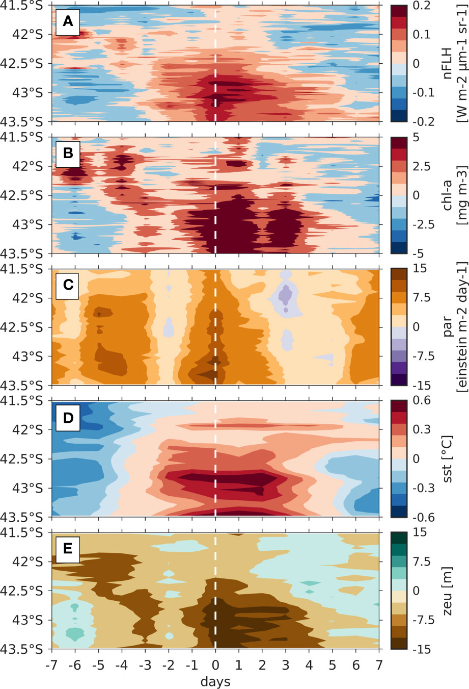
Figure 3 Hovmöller diagrams averaged from the 16 HBE over the longitude band 72.5°-74°W, and centred on the HBE onset, i.e., on day 0, spanning from day -7 to day +7. The variables correspond to (A) nFLH’ [W m^-2 µm^-1 sr^-1], (B) CHLA’ [mg m^-3], (C) PAR’ [einstein m^-2 day^-1], (D) SST’ [°C] and (E) ZEU’ [m]. Day 0 (white dashed line) denotes the day when the p95 threshold is surpassed on nFLH’. Note that the latitudinal range cover the whole ISC, while HBE are defined within the S-ISC subregion (42.5°-43.5° S; see Figure 1A).

TABLE 3

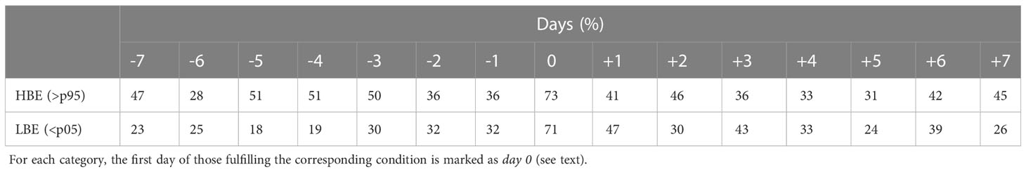
Table 3 Mean spatial availability of sea surface satellite data at 1km horizontal resolution within the southern part of the Inner Sea of Chiloé (S-ISC, i.e. % of gridpoints with valid data) around high biomass events (HBE, i.e., days for which the mean spatial nFLH’ signal is above the p95 threshold) and low biomass events (LBE, i.e., days for which the mean spatial nFLH’ signal is blow the p05 threshold).

3.2 Mesoscale conditions leading to HBEs

Focusing on the mesoscale, Figure 4A shows the temporal evolution of the spatial average of atmospheric fields within S-ISC along the period between days -7 and +7 (anomalies/absolute values on the left/right y-axis), whereas Figure 4B exhibits the corresponding maps of the analysed fields, including MSLP’, a field already shown in Figure 2B. To facilitate the interpretation of this figure, Supplementary Figure 3 provides the absolute values of this sequence of fields: around S-ISC, the MSLP field fluctuates around 1016 hPa according to the transit of the migratory anticyclone; the 10m wind tends to have easterly and southerly components (positive values); PAR is in general higher to the Northeast and exhibits a strong inter-daily variability; and Tx is higher over land than over sea. As shown in Figure 4A, first panel, the positive SLP’ peaks in S-ISC reach between 1 and 2 hPa, interrupted by slightly negative disturbances ​​on days -3 and +3 (the corresponding DJF absolute mean value of ~1016 hPa is denoted by a horizontal black line). Figure 4A, second panel, shows that Tx’ increases gradually, reaching its peak of ~2°C on day -3. Thereafter, Tx’ remains relatively constant until day +7 with values spanning between 1 and 2°C. This translates into absolute values of Tx above 14°C, peaking at ~16°C on day -3 (absolute values on the right-hand side y-axis scale). As revealed by the black contours in Figure 4B, the area over land surrounding S-ISC exhibits a similar temporal Tx’ pattern as that of S-ISC, but showing higher values. Indeed, Chiloé Island (the main island shown) ​​reaches a Tx’ peak of ~3°C on day -3. In Figure 4A, third panel, PAR’ shows in general positive values, with a local maximum exceeding 11.7 einstein m^-2 day^-1 on day 0. Mimicking MSLP’ (Figure 4A, first panel) and as already described for Figure 3C, PAR’ exhibits three pulses of positive anomalies around 10 einstein m^-2 day^-1, separated by local minima lasting ~1 day on days -2 and +3. In absolute values, PAR values around 53 einstein m^-2 day^-1 dominate during the 15-days sequence, with peaks reaching ~60 einstein m^-2 day^-1. As shown in Figure 4B, in general, these conditions do not seem to be confined to ISC, except on day 0 when maximum PAR values are restricted to the 72°-74° W band, extending from the Moraleda channel (around 44°S) northward. Concerning wind at 10m, an increase in both the zonal and meridional components (U10’ and V10’ shown in Figure 4A, fourth and fifth panels, respectively) is evident towards day 0. Negative U10’ indicates anomalous easterly flow that peaks at nearly -0.7 m s^-1 on day -4, decelerating and changing sign towards ~0.4 m s^-1 on day 0. The DJF average for absolute U10 in S-ISC is positive and slightly lower than 2 m s^-1; hence, this result implies that westerlies are subtly enhanced on day 0. On the other hand, the DJF average for absolute V10 in S-ISC is ~0 m s^-1, so any deviation represents an increase in wind magnitude. In this case, V10’ peaks slightly above 3 m s^-1 on day 0. Therefore, while absolute wind –embedded within the mid-latitude westerlies– blows from the SW, we infer that the anomalous wind blows from the SE between days -7 and -2, and from the SW between days -1 and +1. This is confirmed in Figure 4B. Beyond S-ISC, the magnitude of U10’ is about a quarter of V10’, so that anomalous wind is mostly southerly, a pattern that is clearly observed between days -4 and +2 in Figure 4B. All in all, these atmospheric conditions seem to contribute to the positive nFLH’ values in S-ISC that define the HBEs and were described in Figure 2A. In order to highlight the spatial correspondence between the anomalous atmospheric conditions and high nFLH’ values, green dots were plotted where nFLH’>0.1 W m^-2 µm^-1 sr^-1. Low nFLH’ values (nFLH’<-0.1 W m^-2 µm^-1 sr^-1) are indicated by blue dots in Figure 4B. Here, the positive nFLH’ peak within S-ISC on day 0 is unambiguous. The corresponding time series is shown in Figure 5A, first panel.

FIGURE 4

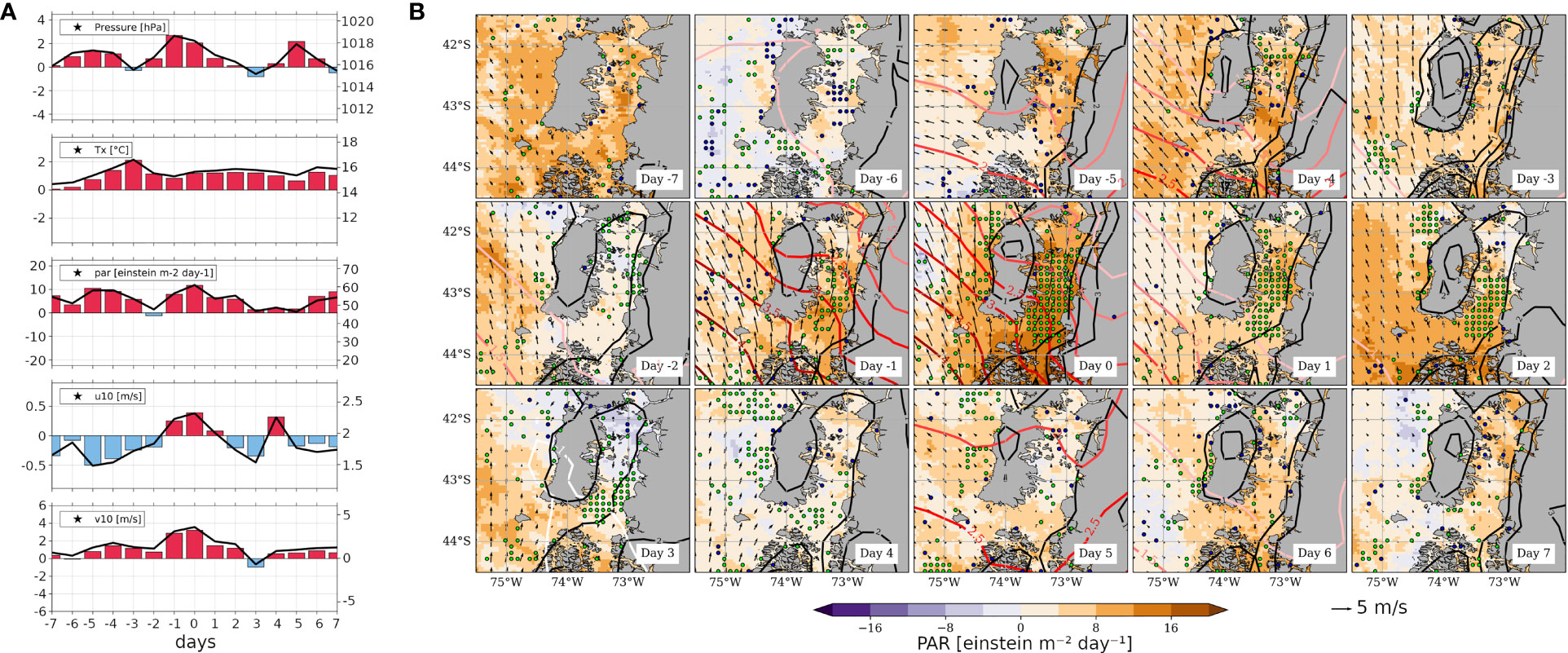
Figure 4 (A) Composite time series averaged from the 16 HBE within the S-ISC subregion (42.5°-43.5° S; see Figure 1A) for a sequence centred on the HBE onset, i.e., on day 0, spanning from day -7 to day +7. Variables correspond to MSLP [hPa], Tx [°C], PAR [einstein m^-2 day^-1], and U and V components of wind at 10m [m s^-1]. The right-hand y-axis of each panel shows the absolute values on solid black lines centred around the mean DJF value (central horizontal line), while the left y-axis shows the positive (negative) SY-IS anomalies on red (blue) bars centred around 0. (B) As Figure 2A, but showing PAR’ (shaded, see colour scale), MSLP’ (reddish contours every 0.5 hPa), Tx’ (black contours every 1°C), 10m wind (black vectors, reference vector below the figure), and nFLH’ (green [blue] dots depict gridpoints with nFLH’>0.1 [nFLH’<-0.1] W m^-2 µm^-1 sr^-1).

FIGURE 5

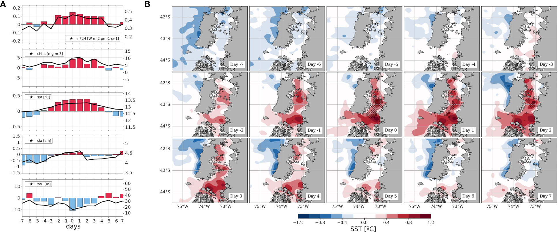
Figure 5 (A) Composite time series averaged from the 16 HBE within the S-ISC subregion (42.5°-43.5° S; see Figure 1A) for a sequence centred on the HBE onset, i.e., on day 0, spanning from day -7 to day +7. Variables correspond to nFLH [W m^-2 µm^-1 sr^-1], CHLA’ [mg m^-3], SST’ [°C], SLA [cm] and ZEU [m]. The right-hand y-axis of each panel shows the absolute values on solid black lines centred around the mean DJF value (central horizontal line), while the left y-axis shows the positive (negative) SY-IS anomalies on red (blue) bars centred around 0. (B) As Figure 4B, but showing SST’ (filled contours, see colour scale), ZEU (for graphical convenience with respect to the SST’ pattern, crosses (dots) depict shoaling (deepening) anomalies below -14m (above 14m)).

Similarly to Figure 4, time series of spatial averages along with regional composite fields are shown in Figures 5A, B, respectively, but in this case for oceanic variables. As in the previous figure, to facilitate the interpretation, Supplementary Figure 4 provides the absolute values of this sequence of fields. Therein, we observe that S-ISC shows in general lower SST than the surrounding ocean (shaded colours), but this condition weakens around day 0; and that the ZEU’ shoals considerably from day -6 towards day 0, reaching -10 m. In Figure 5A, the first and second panels exhibit the evolution for nFLH’ and CHLA’ within S-ISC, already summarised in the description of the Hovmöller diagrams of Figures 3A, B. Specifically, nFLH’ and CHLA’ time series of SY-IS anomalies (absolute values) peak at ~0.15 (~0.5) W m^-2 µm^-1 sr^-1 and ~5 (~11) mg m^-3 on day 0 and +1, respectively, as read at the y-axis on the left-hand (right-hand) side. In Figure 5B, the SST’ sequence exhibits a “warm pool” within S-ISC, while negative values dominate throughout the analysed period beyond ISC, except for Boca del Guafo, where a warm anomaly is also observed between days 0 and +2. In fact, as shown in Figure 5A, third panel, the temporal envelope of positive SST’ within S-ISC lasts for ~1 week and is symmetric with respect to day 0. In particular, the SY-IS peak reaches ~0.4°C (absolute SST: 13.5°C) on day +2. During the analysed time window, the absolute SST mean is ~3°C colder than the mean of maximum air temperature (Tx). It is noteworthy that the warming pattern in S-ISC is different in Tx’ and SST’ (Figure 5A), namely that Tx’ remains nearly constant, whereas SST’ increases and decreases around day 0, reaching its DJF average value on day +5. Figure 5A, fourth panel, shows that the anomalies of sea level altitude (SLA’, see Table 1) within S-ISC increases towards day 0, with slight positive values ​​between days -1 and +1, which correspond to absolute values ​​close to the DJF average of 4.5 cm. The anomalies of surface oceanic currents derived from SLA (not shown) confirm that anticyclonic (cyclonic) anomalies are related to positive (negative) SLA anomalies. While offshore Chiloé Island the anomalies are relatively small, the strongest current anomalies are observed in S-ISC. These indicate slight circulation changes that we interpret as a reduction in the magnitude of the surface ocean current that, in absolute terms, flows towards S-ISC. However, due to the restricted representativeness of actual currents by geostrophic currents within ISC and the small magnitude of the anomalies therein, these fields are not further analysed. Figure 5A, lower panel, reveals a shallower-than-normal ZEU in S-ISC, with ZEU’ values down to -10 m, between days -1 and +3. This period corresponds to the most negative anomalies within the 15-days sequence, preceded by a subtler one between days -5 and -3. In absolute values, ZEU reaches a depth of ~16 m on day 0, while it deepens towards day +5 reaching ~32 m, thus approaching the DJF average of ~35 m. In Figure 5B, the crosses mark gridpoints where ZEU<14 m. A remarkable result is that the shallow ZEU’ pattern is restricted to S-ISC, where it seems to spatially agree with the SST’ pattern.

3.3 Modulation by the MJO

After examining the characteristic field patterns associated with HBE, this subsection shows the modulation of the MSLP’ and nFLH’ fields by the MJO. Figure 6A depicts the composites for each MJO phase computed from all days classified as MJO-active within the analysed period. Red colours denote areas where nFLH’ is positive, indicative of increased phytoplankton biomass. In S-ISC, active MJO phases 4, 6, and 7 are related to the highest nFLH’ values. In the case of active MJO phases 4 and 6, a NE-SW MSLP’ gradient is apparent, resembling the synoptic configuration described for the HBEs on their day 0 (Figure 2). Hence, the association between high nFLH’ values and a migratory anticyclone to the southwest is reinforced by this complementary approach, which is not based on nFLH’ thresholds but on teleconnected tropical-extratropical climate variability. In the case of active MJO phase 7, a subtle MSLP’ NW-SE gradient is suggested. Therefore, the associated high nFLH’ values in this phase seem to be rather a consequence of the persistence of the pattern associated with the preceding active MJO phase 6.

FIGURE 6

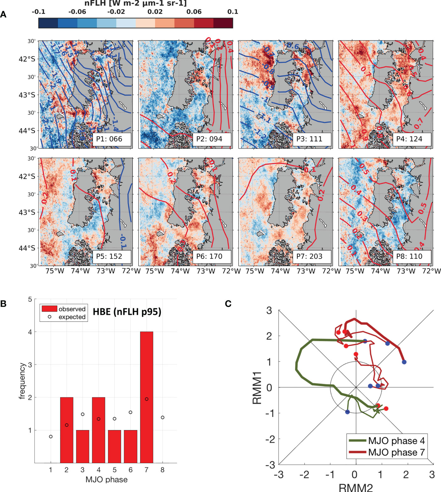
Figure 6 (A) Composite of nFLH’ (SY-IS anomalies, red/blue shaded for positive/negative values [W m^-2 µm^-1 sr^-1]; see colour scale) and MSLP’ (SY-IS anomalies, red/blue contours for positive/negative anomalies every 0.1 hPa) for active MJO phases (RMM index amplitude greater than 1; reference period: DJF 2003-2019); the box in the lower right corner of each panel indicates the respective MJO phase and the number of days used in the composite. (B) red bars: Histogram of the 11 observed HBEs for which the corresponding day 0 coincides with an active MJO phase, grouped by MJO phases. The empty circles show the expected frequency of 11 events if they followed the climatological distribution of active MJO phases for DJF 1975-2020. (C) Trajectories in the MJO RMM diagram for each HBE whose day 0 occurred on active MJO phases 4 and 7 (green and brown curves, respectively); day 0 and day -14 are identified by a red and blue circle, respectively. The bold curves indicate the trajectories of the two case studies culminating respectively on January 19, 2019 (MJO active phase 4, green curve) and January 23, 2013 (MJO active phase 7, brown curve).

In total, 11 out of the 16 identified HBEs (~69%) occur during active MJO phases (considering their respective days 0). The corresponding histogram (Figure 6B) reveals that 4 of those 11 events (~36%) concentrate on phase 7, followed by 2 (~18%) on both phases 4 and 2. Such distribution is remarkably different from that expected from the climatology of MJO active phases for 11 events (shown by circles). Due to the restricted number of cases, a chi-squared test can not be applied to these distributions to explore the significance of such difference. Complementing our previous analysis, Figure 6C shows the 15-day-long trajectories in the MJO phase-diagram for those HBEs that culminate on active MJO phases 7 and 4 (brown and green lines, respectively; blue circles: day -14, red circles: day 0). While the two cases occurring on MJO 4 exhibit rather erratic trajectories, most HBEs that culminate on MJO phase 7 exhibit a persistence of well-established active MJO conditions that evolve and intensify from their start on MJO phases 4-5 14 days before. This is a key aspect when aiming at enhanced forecasting opportunities regarding HBEs. As shown in Supplementary Figure 5 and Table SMT1, a further result that reinforces the possible connection of phytoplankton dynamic within S-ISC with the MJO is that, in contrast to the distribution obtained for HBE, LBE occurring during active MJO (14/18, ~78%) tend to concentrate on MJO phase 5 (4/14, ~29%). Again, this result is in agreement with the predominating negative nFLH’ values observed over S-ISC for the composites computed over MJO active phases (Figure 5).

3.4 Case studies

The analysis of two case studies builds upon similar figures as the ones produced for the composites, in which case the average fields (composites) of all HBEs were computed (Figures 4, 5). In this section, the anomaly fields corresponding to the 15-days sequence for two single events are described. The selected HBEs correspond to January 17, 2019 and January 23, 2013. As shown in Table 2, these events culminated during active MJO phases 7 and 4, respectively. Moreover, beyond the pattern of increased phytoplankton biomass that both cases reveal, in-situ evidence indicates that both events were related to HAB in S-ISC.

3.4.1 Case study: January 17, 2019

The HBE identified on January 17, 2019 is presented in a similar way as the previous composites, i.e., through spatially-averaged time series for S-ISC (Figures 7A, 8A) along with maps of atmospheric and oceanic variables, using both anomalies and absolute values (Figures 7, 8 and Supplementary Figures 6, 7, respectively). Figure 7A depicts a similar evolution of the time series of the studied atmospheric variables for S-ISC as that of the composite, but in this case short disturbances are observed in-between, so that positive anomalies are less persistent than in the composite sequence. Here, the MSLP’ peak is reached on day 0 (instead of day -1, as in the composite), showing absolute values ​of almost 1028 hPa and anomalies surpassing twice the values observed in the composite. This signal corresponds to the migratory anticyclone crossing the study area, which is well depicted in the map sequence that shows absolute values (Supplementary Figure 6). However, as in the composite, the map sequences on Figure 7B and Supplementary Figure 6 show that the MSLP’ gradient towards the Southwest maximises on day 0. The negative MSLP’ values, with local minima on days -2 and +3, correspond to a short-lived cyclonic (frontal) system restricted to the western flank of the migratory anticyclone (Figure 7). The disturbances associated with that cyclonic system led to precipitation over ISC. In particular, on day -2 (January 15, 2019), a coastal station within S-ISC (Quellón, 43.1086°S, 73.6119°W) registered 4.4 mm liquid precipitation (not shown). Regarding Tx’, beyond the local maximum during days -4 and -3, the global peak occurs during days +1 and +2, reaching anomalies of ~3°C and absolute values ​​of almost 18°C (Figure 7A). The Tx’ peak within the S-ISC is around 3°C, of greater magnitude than that of the composite signal, and occurs on days +1 and +2, in synchrony with the signal over land encompassing the whole ISC (Figure 7B). In Figure 7A, S-ISC exhibits PAR maxima up to 67 einstein m^-2 day^-1; positive PAR’ anomalies are interrupted by synoptic intermittencies that lead to negative anomalies ​​lasting 1-2 days. In general, the anomalies are twice those observed in the composite. In this case, evident negative PAR’ anomalies over ISC on days -6, -2, +3, +4, and +7 (Figure 7B) correspond also roughly to local minima in the composite (Figure 4B). As mentioned above, such local minima are caused by brief synoptic instabilities. With respect to 10m wind, its components exhibit co-variability, with V10’ doubling U10’ in magnitude (Figure 7A). This proportion does not hold for absolute values, because –as we could observe for the composite– the DJF averages for the zonal and meridional components are different. To correctly interpret these signals, a comparison between Figure 7 and Supplementary Figure 6 is suggested. For U10, both the decrease in negative anomalies and the increase in positive anomalies translate into an increase in the absolute magnitude of westerly wind. However, for V10, the decrease in negative anomalies results in a weakening of actual northerly wind, whereas the increase in positive anomalies results in a strengthening of actual southerly wind. Thus, each of the three pulses observed during days -6/-2, -2/+3, and +3/+5 represent veering and backing cycles (i.e., increase in the zonal component along with decrease, direction change, and increase in the meridional component, followed by the reverse process). Again, this wind pattern is directly related to the cyclonic disturbances that interrupt the prevailing southerly wind (Figure 7B).

FIGURE 7

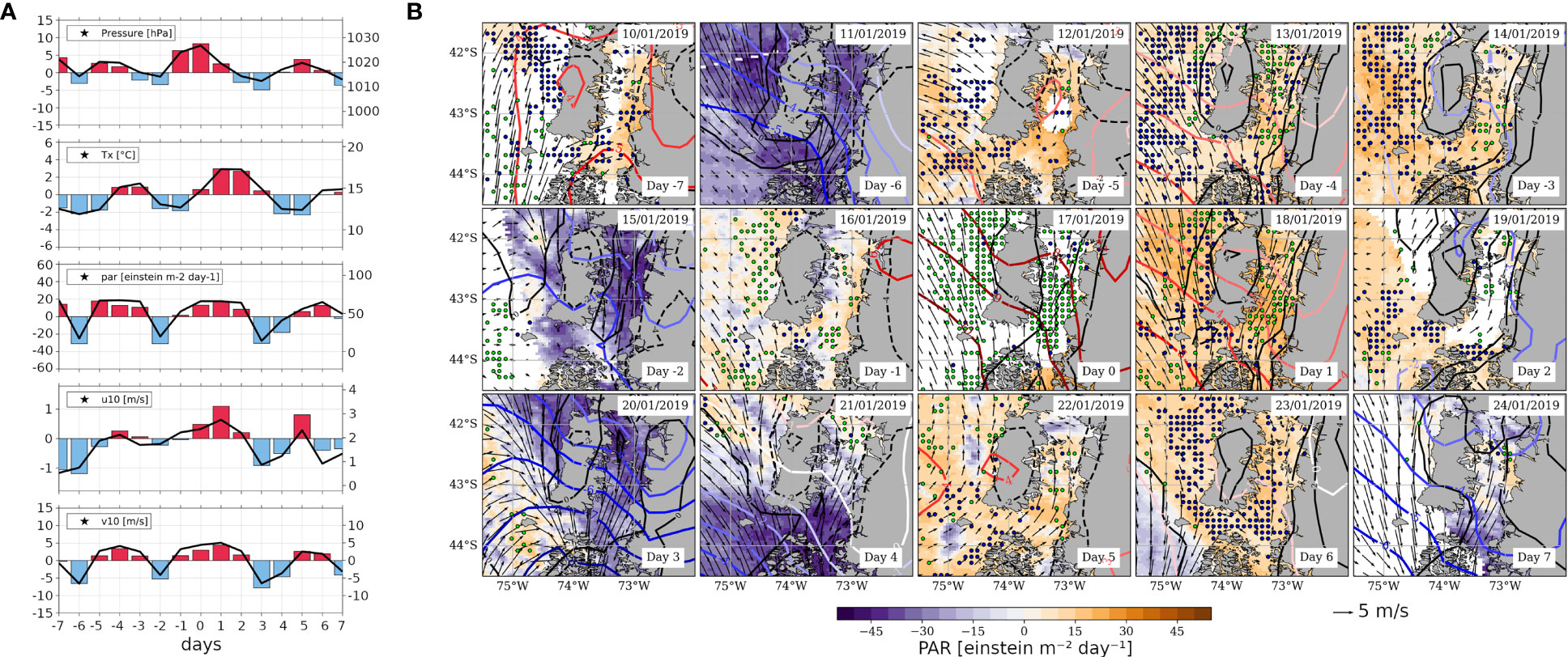
Figure 7 As Figure 4, but referred to the case study around the HBE of January 17, 2019 (day 0). (A) Time series calculated as field averages within the S-ISC subregion (42.5°-43.5° S; see Figures 1A) for a sequence of days centred on the HBE onset, i.e., on day 0, spanning from day -7 to day +7. Variables correspond to MSLP [hPa], Tx [°C], PAR [einstein m^-2 day^-1], and U and V components of wind at 10m [m s^-1]. The right-hand y-axis of each panel shows the absolute values on solid black lines centred around the mean DJF value (central horizontal line), while the left y-axis shows the positive (negative) SY-IS anomalies on red (blue) bars centred around 0. (B) Maps centred on day 0, spanning from day -7 to day +7, showing PAR’ (shaded, see colour scale), MSLP’ (reddish contours every 1 hPa), Tx’ (black contours every 2°C), 10m wind (black vectors, reference vector below the figure), and nFLH’ (green [blue] dots depict gridpoints with nFLH’>0.1 [nFLH’<-0.1] W m^-2 µm^-1 sr^-1).

FIGURE 8

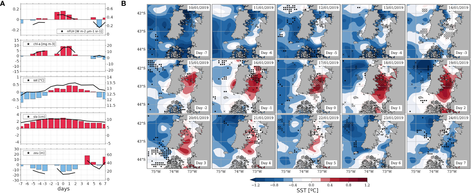
Figure 8 As Figure 5, but referred to the case study around the HBE of January 17, 2019 (day 0). (A) Time series calculated as field averages within the S-ISC subregion (42.5°-43.5° S; see Figures 1A) for a sequence of days centred on the HBE onset, i.e., on day 0, spanning from day -7 to day +7. Variables correspond to nFLH [W m^-2 µm^-1 sr^-1], CHLA [mg m^-3], SST [°C], SLA [cm] and ZEU [m]. The right-hand y-axis of each panel shows the absolute values on solid black lines centred around the mean DJF value (central horizontal line), while the left y-axis shows the positive (negative) SY-IS anomalies on red (blue) bars centred around 0. (B) Maps centred on day 0, spanning from day -7 to day +7, showing SST’ (filled contours, see colour scale), ZEU' [for graphical convenience with respect to the SST’ pattern, crosses (dots) depict shoaling (deepening) anomalies below -14m (above 14m)].

Regarding the time series of oceanic variables (Figure 8A), nFLH within S-ISC (first panel) maximises between days -1 and +2, with anomalies and absolute values around 0.16 and 0.46 W m^-2 µm^-1 sr^-1, respectively. This temporal evolution is also shown by CHLA (second panel), where the absolute values ​​reach almost 20 mg m^-3 on days 0 and +1. Therefore, in this event, the nFLH and CHLA signals are coupled. We can notice that data unavailability might be presumably linked to the cyclonic disturbances mentioned above, which lead to enhanced cloudiness. Warming in S-ISC is evident from day -2 to day +5, reaching anomalies and absolute values of ~0.5°C and ~13.5°C, respectively (third panel). The overall SST’ maximum is observed on day +2, contrasting with the composite signal that shows the peak on day +1 (Figure 5A). The map sequence of anomalies (Figure 8B) clearly shows that this warming is restricted to S-ISC. However, in absolute values, SST over S-ISC remains colder than in the surrounding ocean during the 15 days analysed (Supplementary Figure 7). Regarding SLA time series (Figure 8A, fourth panel), positive anomalies persist during this period, reaching absolute values higher than 10.4 cm. In this context, ZEU (Figure 8A, fifth panel) reveals a shallower-than-normal euphotic layer (denoted by black crosses) that reaches absolute values ​​of ~10 m on day 0 (Figure 8A, lower panel). While a shallowing ZEU is restricted to S-ISC and coincides in space and time with the peak in nFLH and CHLA, a deepening ZEU (black dots) is apparent outside S-ISC, particularly on day +3 around 43.5°S in the adjacent coastal ocean (Figure 8B).

From November 2018 to January 2019, in-situ observations of marine currents and hydrographic variables from a mooring deployed at the Boca del Guafo (43.7217°S, 73.85481°W; see Figure 1A) are available (Figure 9). These observations allow us to inspect in depth the water column variability related with particular HBE and LBE identified within this period. Previous to the HBE of January 17, 2019 (green vertical line in Figure 9), northwest currents (indicating outflow from the ISC towards the Pacific ocean) dominate the 15-40m layer, while northeast currents (inflows) are observed in the deeper 40-60m layer. After the HBE, mostly outflows were observed in the 20-60m water column. The thermal structure of the water column confirms the persistent regional surface warming pattern during the ~10 days preceding the HBE. Meanwhile, salinity and oxygen shows a negative anomaly suggesting a decrease before the HBE. These results are consistent with southerly winds producing offshore transport in the surface, which can push fresher surface water out of the ISC. During the days preceding the LBE (i.e., an event that corresponds to nFLH’ values below the p05 percentile, marked by a yellow vertical line in Figure 9) on December 7, 2018, contrasting surface conditions prevailed, in particular an enhanced southern current and relatively low SST, along with relatively high oxygen values. Thus, for both HBE and LBE, these observations reinforce the co-variability of nFLH’ and the studied variables.

FIGURE 9

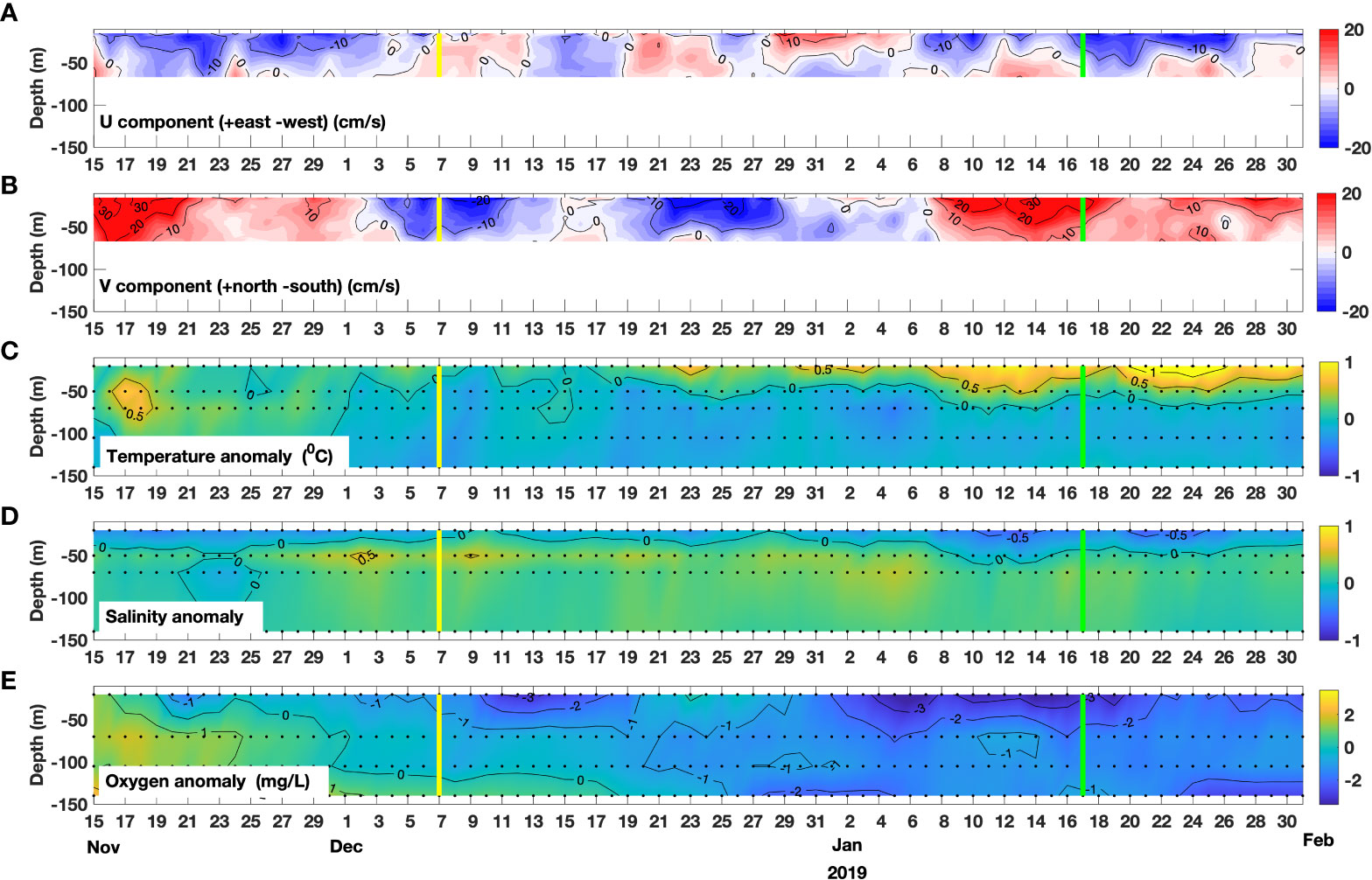
Figure 9 Time series of in-situ ocean variables recorded between November 15, 2018 and January 31, 2019. From top to bottom: (A) zonal component U of the ocean current, (B) meridional component V of the ocean current, (C) temperature anomaly, (D) salinity anomaly, (E) oxygen anomaly.

In terms of the MJO teleconnection, on January 17, 2019, i.e., the day 0 of this HBE, an active MJO phase 4 was recorded (Figure 6C; dimensionless RMM index intensity: 1.1). Hence, the observed high nFLH’ values in S-ISC confirm the expected signal from the MJO composite pattern (Figure 6A). Moreover, 14 days before this date, the MJO exhibited an active phase 6 that developed quickly towards an active MJO phase 4. Such MJO trajectory suggests that the monitoring of this evolution could have been possible in operational terms, with focus on the biological response within S-ISC. Besides, in-situ monitoring within ISC, recorded that the relative abundance of Alexandrium catenella increased between January 15 and 17, 2019 (i.e., days -2 to 0; IFOP, 2019b). Accordingly, and as reported on public press releases (SalmonExpert, 2019; Terram, 2019), the corresponding alert state changed from “moderate precaution/yellow traffic light” (associated with low-to-moderate abundance, as issued on the previous report corresponding to January 2-5, 2019; IFOP, 2019a) to “early warning/orange traffic light”. Therefore, the evidence presented here suggests that, in this case, increased biomass in S-ISC could have been related to a developing HAB.

3.4.2 Case study: January 23, 2013

The HBE identified on January 23, 2013 was also characterised by the evolution of salient atmospheric and oceanic variables (Figures 10, 11, respectively; for absolute values, Supplementary Figures 8, 9, respectively). The first panel of Figure 10A shows absolute MSLP values ​​mostly above 1016 hPa over S-ISC, with positive anomalies throughout the analyzed period, except on days -3 and -2 which exhibit slightly negative anomalies (-1 to -2 hPa). This high MSLP’ signal arises from the migratory anticyclone crossing eastward and resembles the composite pattern (cf. Figures 10B, 4B, respectively). Over S-ISC, Tx’ peaks on day -4 (Figure 10A, second panel), slightly surpassing 8°C, which corresponds to 23.5°C in absolute values. Despite the generally warm conditions during the 15-days sequence, a slight cooling is observed between days +1 and +3, reaching ~14.2°C, i.e., nearly the average DJF value. Over the land surrounding ISC, the Tx signal is in agreement with S-ISC (Figure 10B) and maximizes on day -4 (January 19, 2013), when in fact 32.7°C were recorded at “El Tepual Puerto Montt” weather station (41.4350°S, 73.0978°W; northern edge of Figure 10). This value exceeds by >9°C the value of 23.6°C, reported by the National Weather Directorate (DMC) as a threshold for that station to define extreme Tx events (in particular heat waves, in case of persistence longer than 3 days). Specifically, such threshold corresponds to the smoothed daily 90th percentile for that particular day considering the period 1981-2010. In fact, January 19 corresponds to the peak of a heat wave spanning January 18-21, 2013. These extremely warm conditions affected a wide region extending to the north and south of the study area. Regarding PAR, high values prevail throughout the analysed period, with anomalies and absolute values of ~20 and ~60 einstein m^-2 day^-1, respectively. These values are of similar magnitude as those of the composite (cf. Figures 10A, 4A, respectively). Similar PAR conditions to those found over S-ISC extend over a larger area (Figure 10B and Supplementary Figure 8) except for day +4, when some negative anomalies are shown west of 74°W, in concomitance with northerly wind. The wind pattern sequence behaves similarly to that observed in the companion case study (January 2019) and the composite of all HBEs (Figure 4). Three wind pulses are observed (Figure 10A, fourth and fifth panels); during the second one, U10 increases from day -4 to day 0, while V10 increases from day -2 to day +1. Later, both wind components decrease towards day 4. Throughout almost the whole 15-days sequence, southerly anomalies persist, as also observed in the entire region (Figure 10B and Supplementary Figure 8).

FIGURE 10

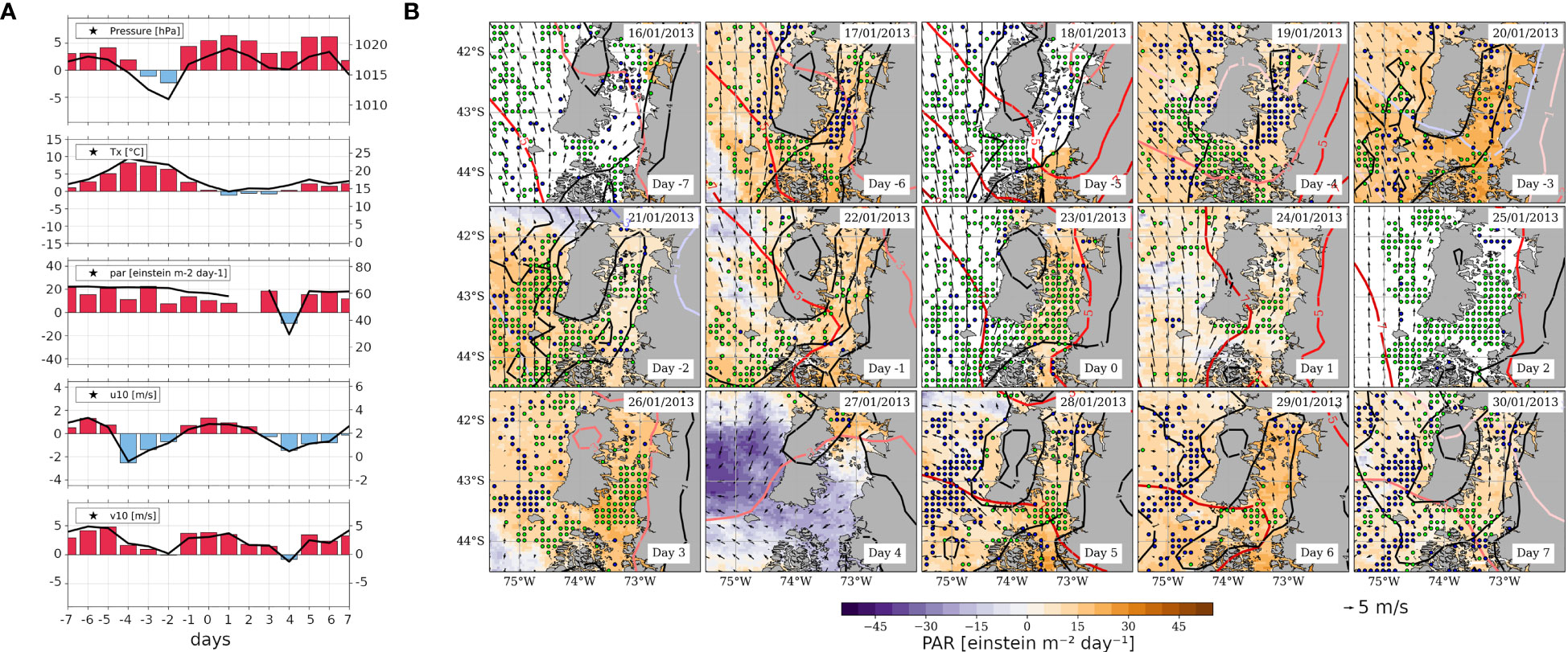
Figure 10 As Figure 4, but referred to the case study around the HBE of January 23, 2013 (day 0). (A) Time series calculated as field averages within the S-ISC subregion (42.5°-43.5° S; see Figures 1A) for a sequence of days centred on the HBE onset, i.e., on day 0, spanning from day -7 to day +7. Variables correspond to MSLP [hPa], Tx [°C], PAR [einstein m^-2 day^-1], and U and V components of wind at 10m [m s^-1]. The right-hand y-axis of each panel shows the absolute values on solid black lines centred around the mean DJF value (central horizontal line), while the left y-axis shows the positive (negative) SY-IS anomalies on red (blue) bars centred around 0. (B) Maps centred on day 0, spanning from day -7 to day +7, showing PAR’ (shaded, see colour scale), MSLP’ (reddish contours every 2 hPa), Tx’ (black contours every 3°C), 10m wind (black vectors, reference vector below the figure), and nFLH’ (green [blue] dots depict gridpoints with nFLH’>0.1 [nFLH’<-0.1] W m^-2 μm^-1 sr^-1).

FIGURE 11

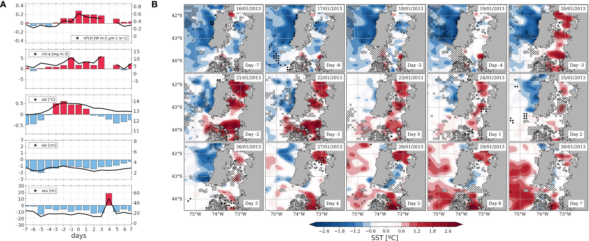
Figure 11 As Figure 5, but referred to the case study around the HBE of January 23, 2013 (day 0). (A) Time series calculated as field averages within the S-ISC subregion (42.5°-43.5° S; see Figures 1A) for a sequence of days centred on the HBE onset, i.e., on day 0, spanning from day -7 to day +7. Variables correspond to nFLH [W m^-2 μm^-1 sr^-1], CHLA [mg m^-3], SST [°C], SLA [cm] and ZEU [m]. The right-hand y-axis of each panel shows the absolute values on solid black lines centred around the mean DJF value (central horizontalline), while the left y-axis shows the positive (negative) SY-IS anomalies on red (blue) bars centred around 0. (B) Maps centred on day 0, spanning from day -7 to day +7, showing SST’ (filledcontours, see colour scale), ZEU' [for graphical convenience with respect to the SST’ pattern, crosses (dots) depict shoaling (deepening) anomalies below -14m (above 14m)].

As in the 2019 case, the 2013 HBE is evident in both the nFLH and CHLA signals (Figure 11A, first and second panels). On one hand, nFLH’ exhibits one peak exceeding 0.2 W m^-2 µm^-1 sr^-1 on day 0, while high values persist at least until day +3. On the other hand, CHLA exhibits positive anomalies throughout the sequence; absolute values remain ​​above the DJF average of ~3.3 mg m^-3, and two peaks of CHLA’ of ~5 mg m^-3 are observed on days -1 and +4. The warming signal revealed by SST’ over S-ISC (Figure 11A, third panel) is more temporally restricted than in the composite of Figure 5, spanning from days -3 to +1 and reaching absolute values ​​of almost 14°C. Nevertheless, the warming signal covers a larger area than in the composite, extending to the whole ISC (Figure 11B). After day +5, S-ISC exhibits negative anomalies, whereas N-ISC and open waters show positive anomalies exceeding 1.2°C (Figure 11B and Supplementary Figure 9). However, in absolute terms, S-ISC remains above the DJF average of ~12.7°C (Figures 11A, third panel). Throughout the period, SLA shows negative anomalies within S-ISC (Figure 11A, fourth panel), reaching absolute values ​of ~3.3 cm on day -2, below the DJF average of ~4.4 cm. A similar signal is shown by ZEU’ over S-ISC (Figure 11A, fifth panel), with negative values reaching down to ~10m except for day +4. In contrast to the pattern observed for the composite (Figure 5), this ZEU signal over S-ISC does not seem to be temporally coupled with the regional oceanic warming signal (Figure 11B).

All in all, this HBE occurred under persisting clear sky conditions, as revealed by the absolute PAR sequence (Supplementary Figure 8). The corresponding day 0 on January 23, 2013, was classified as an active MJO phase 7 (dimensionless RMM index intensity: 2.16). As in the previous case study, this event exhibits the enhanced MSLP’ gradient promoting high nFLH’ values expected from the composite for active MJO phase 7 (Figure 6), suggesting the (at least partial) role of an atmospheric teleconnection behind such atmospheric pattern. After January 22, 2013, in-situ monitoring around 43°15’S, 73°35’W revealed notorious increases in relative abundance of Dinophysis acuminata, Dinophysis acuta, Protoceratium reticulatum, which along with Alexandrium ostenfeldii also exhibited increased cell numbers within the 10-20m layer (IFOP, 2013). All this observational evidence suggests that the conditions reported here might have been linked with developing HABs.

4 Summary, discussions, and conclusions

In this study, we examine the link between atmospheric variability and events of high phytoplankton biomass (HBEs) in the southern Inner Sea of Chiloé in NW Patagonia (S-ISC, Figure 1). In our approach, the seasonal and inter-annual departures of each variable are removed to focus on synoptic-intraseasonal (SY-IS) variability. These events are defined as those events during which the anomalies of normalized fluorescence line height (nFLH’) averaged within S-ISC exceeds its 95th percentile (p95). The nFLH has been reported as a more robust proxy than chlorophyll-a (CHLA) for phytoplanktonic biomass concentration in this area (Lara et al., 2017; Vásquez et al., 2021). A total of 16 HBEs were identified for the austral summer from 2003 to 2019; some of which might have led to harmful algal blooms (HABs).

Some phytoplankton species are particularly sensitive to environmental factors such as nutrient availability or solar irradiance conditions for their multiplication (e.g., Sapiano et al., 2012). Human activities might contribute to modifying nutrients, e.g., due to eutrophication associated with fertilisation processes stemming from the aquaculture industries (Iriarte et al., 2013; Mayr et al., 2014; Olsen et al., 2014; Olsen et al., 2017). Different conditions of light availability mostly modulated by natural processes can cause changes in phytoplankton biomass. In ISC, it is known that the annual cycle of solar irradiance is a key factor for phytoplankton activity (e.g., González et al., 2010). In particular, Pizarro et al. (2000) found that phytoplankton assemblages within the ISC, unlike those found in the fjords towards southernmost Patagonia, are not habituated to low light conditions; thus, a reduction in CHLA is observed in ISC during the winter months. In this context, it is relevant to highlight that environmental characteristics such as atmospheric and oceanic circulation and stability as well as solar irradiance are strongly controlled by large-scale and regional atmospheric forcing. Thus, interannual climate variability (a phenomenon that lies beyond the scope of this paper) has been proposed as a relevant driver of blooms in the ISC. The most salient climate modes that have been studied in this respect are El Niño-Southern Oscillation (ENSO) and the Southern Annular Mode (SAM). In this regard, summer 2016 was recorded as an exceptional season: ENSO and SAM exhibited their positive phases, leading to sustained very dry conditions and enhanced solar radiation in Western Patagonia, which in turn caused a HAB of Pseudochattonela cf. verruculosa and a major socio-environmental crisis (Garreaud, 2018; León-Muñoz et al., 2018). On top of this interannual variability, synoptic-scale disruptions (i.e., in the timescale up to ~10 days) might induce changes to these characteristics and favour conditions for biologic activity, particularly by increasing limiting growth factors. Such a mechanism has been proposed for winter blooms in a Patagonian fjord (Montero et al., 2017), specifically due to a cyclonic system causing vertical mixing in the water column that, in turn, increases nutrient availability in the surface layer. Hence, the question whether HBE are related to such synoptic-to-intraseasonal (SY-IS) atmospheric patterns, arises naturally.

Therefore, in this work, we focus on transient SY-IS disturbances that exhibit abnormally high CHLA or nFLH levels, taken as proxies for enhanced phytoplanktonic biomass. We base our research upon the exploration of reanalyses and satellite data. The mean atmospheric and oceanic patterns (composite) that develop along a sequence of 15 days (days -7 to +7) centred at the beginning of HBEs (day 0) reveal, as their most salient feature, a migratory anticyclone that progresses eastwards south of the study area. In general terms, migratory anticyclones are an atmospheric forcing over southern South America that modulates the environment on the synoptic scale. Several studies have addressed migratory anticyclones over subtropical and mid-latitudes of South America, particularly addressing their dynamics and impacts on the atmospheric conditions. In summer, the South Pacific subtropical anticyclone (a climatological feature) is displaced a few degrees further south of its climatological position (Rahn and Garreaud, 2014). Therefore, migratory anticyclones (transient systems) tend to be more frequent and persistent, possibly exceeding the synoptic timescale and eventually leading to intraseasonal, longer-lasting blocking patterns, such as the observed pattern in this study. Mid-latitude migratory anticyclones have been related to the formation of coastal lows along the coast of central and south Chile (Garreaud et al., 2002; Garreaud and Rutllant, 2003), stable atmospheric conditions, enhanced solar radiation, and the intensification of easterly downslope winds over the Andes (Montecinos et al., 2017). These conditions promote the occurrence of heat waves in central and south Chile (Demortier et al., 2021) and lead, therefore, to further impacts, such as large wildfires (McWethy et al., 2021). Moreover, migratory anticyclones have been particularly studied in connection with their promotion of upwelling-favorable winds along oceanic eastern boundaries, particularly in south-central Chile, where they are projected to become more (less) frequent in higher (lower) latitudes by the end of the 21st century (Aguirre et al., 2019).

In this study, we show some impacts of migratory anticyclones over the mid-latitude of West Patagonia, especially those related to ocean-atmosphere interactions. The analysis of the atmospheric composite based on all HBEs (Figures 3, 4) reveals that the eastward progression of migratory anticyclones enhances the gradient of mean sea level pressure anomalies (MSLP’) towards the day of occurrence of HBE (day 0), with a marked NE-SW direction. Consistently, southerly wind intensifies, reaching a maximum on day -1, while a subtle easterly anomaly also intensifies on day -5, turning later into a westerly anomaly that peaks on day 0. These conditions lead to cloudless skies and enhanced solar photosynthetically-active solar radiation (PAR), whose anomalies maximise over S-ISC on day 0. On days -3 and +4, negative PAR’ values might be associated with enhanced cloudiness that prevents the full penetration of radiation, thus leading to gaps in the nFLH data. As revealed by Figure 2, such a mean signal of enhanced cloudiness would be associated with a coastal low propagating southward and culminating on day -3, and a frontal system migrating eastwards on day +4, respectively. Nevertheless, throughout the 15-days sequence, the environmental evolution is embedded within persistent positive anomalies of maximum air temperature (Tx).

In the ocean (Figures 3, 5), the described atmospheric evolution results in the development of a positive envelope of sea surface temperature anomalies (SST’) and the shoaling of the euphotic layer (ZEU). These conditions are consistent with an increased atmospheric stability, enhanced PAR, and higher Tx, and also suggest relatively more stratified and thus more stagnant oceanic conditions in S-ISC, which could induce longer residence times in the area. In other words, this configuration might lead to a weakened oceanic circulation, promoting a warm water pool in S-ISC. In summary, as schematized in Figure 12, we hypothesise that biological activity is promoted within a shallower-than-normal mixed layer embedded in a warmer and more stratified water column due to increased solar irradiance. Specifically, the local PAR’ maximum around day -5 seems to initiate the heating of the ocean surface, which the local PAR’ maximum on day 0 further intensifies (Figures 2, 5). Thereafter, positive SST’ values persist until day +3, suggesting the characteristic timescale for the oceanic response to such enhanced solar radiation. Altogether, the evolution of the variables shown in this study reveal the general conditions that seem to promote high concentrations of phytoplankton biomass. Moreover, HBEs (defined on nFLH’) tend to exhibit CHLA’ exceeding its own p95. As shown in Table 2, both kinds of events tend to have a correspondence in time with a lead/lag within the range of -3 to +3 days. As mentioned above, both variables serve as a proxy to quantify the abundance of phytoplankton biomass at the ocean surface in S-ISC, a condition that depends on complex space-time interactions between physical, chemical, and biological processes.

FIGURE 12

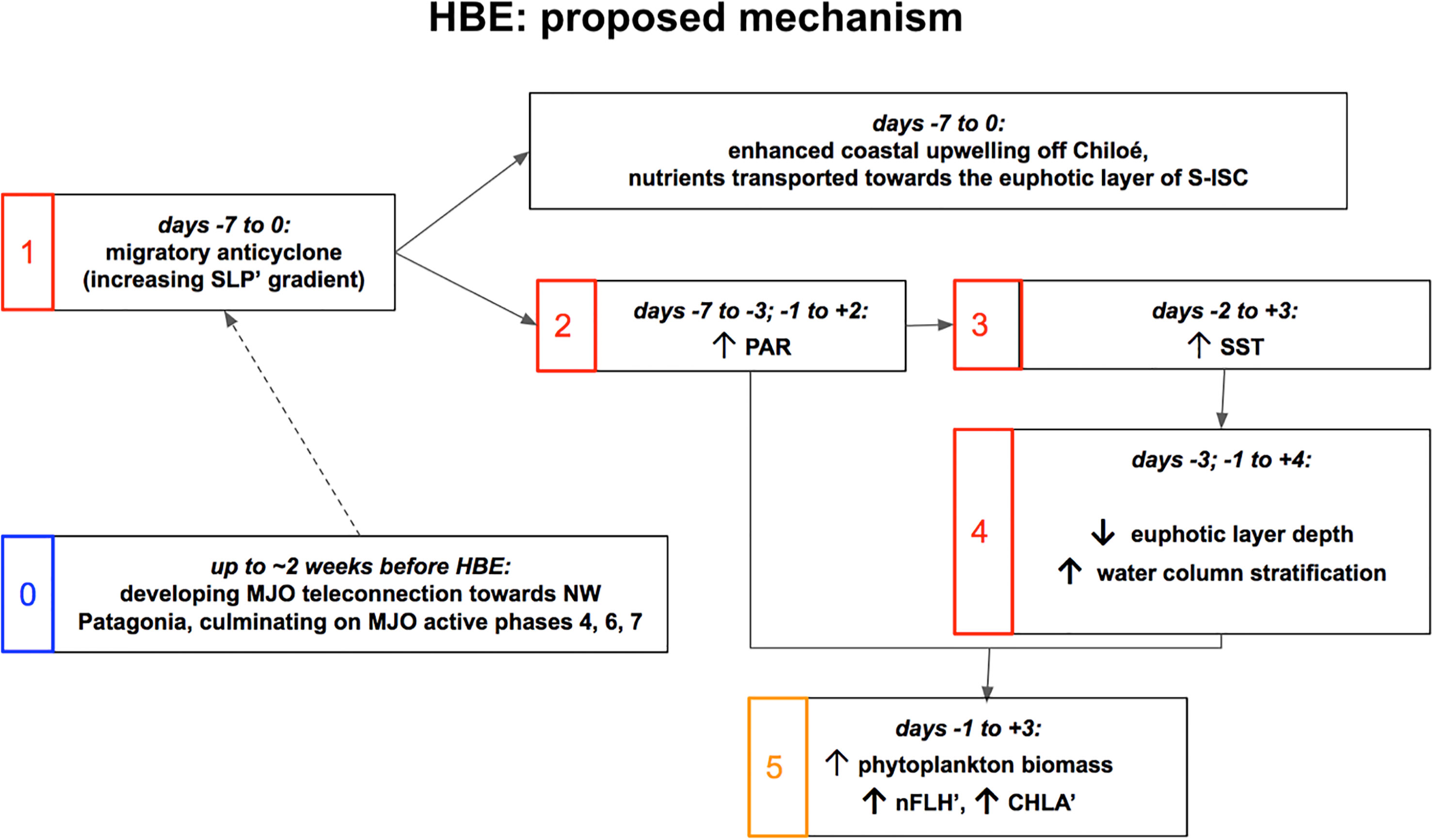
Figure 12 Schematic mechanism proposed for the average signal of the occurrence of HBE in association with the atmospheric forcing imposed by a migratory anticyclone over the study area. For complementary spatio-temporal information, please refer to the Hovmöller diagrams of Figure 3.

Throughout our analysis, we present the mean conditions calculated from a collection of events. Thus, they might represent “idealized situations”. To deliver insights into the particularities of single events, we included two case studies. On the one hand, the sequence around January 17th, 2019 (case study 1) exhibits transient disturbances related to frontal systems on days -6, -2, +3 (Figure 7B), which are not evident on the composite sequence (Figure 4B). Furthermore, it does not show its maximum PAR’ signal around day 0. For this reason, precipitation and its impacts should be considered as further drivers of this particular HBE. This aspect is discussed below. Despite this discrepancy, the warming SST’ pattern for this case study (Figure 8B) is similar to that observed in the composite (Figure 5B). On the other hand, the sequence around January 23rd, 2013 (case study 2; Figure 10B) follows the mean SLP’ evolution of the composite sequence, although it does not exhibit the strongest SLP’ gradient on day 0. Additionally, the corresponding evolution of SST’ for this particular case (Figure 11B) shows a scattered pattern that is more persistent than the composite sequence. All in all, these exercises underscore that a diversity of specific characteristics might be expected for each event.

Although not evident from our analysis, we speculate in Figure 12 that these conditions could be further favoured by a nutrient-rich environment promoted during the previous days by nutrient inflow induced by enhanced currents towards S-ISC either from the Moraleda Channel (to the south of S-ISC) or from the upwelling area off the Pacific coast (to the west of S-ISC). While the effect of the southerly wind on the ocean surface of the ISC has not been thoroughly addressed in this study, in the coastal open zone west of Chiloé Island, it favours the coastal upwelling of deep, nutrient-rich waters. During summer, upwelling-favorable winds extend polewards, reaching the latitude of the study area (Aguirre et al., 2019; Narváez et al., 2019). Furthermore, southerly wind seems to establish ocean currents entering the Boca del Guafo towards S-ISC, as observed for the 2019 case study in the 40-60m layer in Figures 9A, B. Such currents can produce a nutrient transport into the study area, as proposed by Pérez-Santos et al. (2019), and therefore could be linked to increases in the local phytoplankton biomass (Vásquez et al., 2021). Indeed, Supplementary Figure 10 shows mean Ekman suction/pumping anomalies (i.e., anomalous upward/downward vertical motion, respectively) for the 15-days sequence centred on the 16 HBEs. On days -5 and -3, we observe a well-defined dipole of SW-NW positive-negative anomalies: Ekman suction (i.e., upwelling) in open ocean waters just west of Boca del Guafo and Ekman pumping (i.e., downwelling) over S-ISC. Although caution must be kept when interpreting this process in an area with such complex bathymetry and topography, this pattern supports the upwelling of nutrients in the open sea and their transport by the subsurface current towards S-ISC. However, the mechanism shown here in the SY-IS timescale is possibly complementary to that shown by Pérez-Santos et al. (2019), which was described for a longer timescale. Pérez-Santos et al. (2019), in their Figure 11, show some summer events of persistent high CHLA levels along the west coast of Chiloé and within the ISC which occur embedded in colder-than-normal conditions (i.e., negative SST’), and relate them to strong and long-lasting total coastal upwelling which would transport nutrients to the surface and phytoplanktonic organisms to the fjords and channels of Patagonia from the waters west of Chiloé Island.

Indeed, over areas where phytoplankton activity might be limited by sunlight but not by nutrient availability, physical processes such as vertical mixing promoted by atmospheric instability (e.g., related to migratory cyclones) tend to prevent blooms as enhanced cloud cover leads to insufficient PAR and, moreover, the algal cells are moved to deeper ocean layers where sunlight is insufficient for their growth (Sverdrup, 1953; Venables & Moore, 2010). On the contrary, if sunlight is not a primary limiting factor, phytoplankton activity might be limited by nutrients that might be available deeper in the water column (e.g., Le et al., 2022). In the present study, active mixing in the upper ocean occurring some days before a migratory anticyclone establishes could homogenise properties within the upper layer of the ocean, preceding periods of high atmospheric stability (weak mixing). Water column mixing would make nutrients (nitrogen, phosphorus and silicate) available in the ocean upper layer. In S-ISC, as the water supply from the subsurface ocean is richer in nitrate and phosphate (less in silicates), dinoflagellates tend to dominate (Martínez et al., 2015, and references therein). If subsequent stable periods are long enough, bio-optical structures could form within a well-mixed ocean upper layer (Carranza et al., 2018). Indeed, such stabilisation of the ocean surface after strong mixing constitutes one of the common mechanisms for blooms in temperate coastal zones of high latitudes (Mann and Lazier, 2013). However, it is this stratification that eventually causes a separation between the algae and their main source of nutrients in deeper waters, leading to short-lived blooms lasting for some days (Iriarte et al., 2007). In this sense, the proposed mechanism is analogous to the “critical depth hypothesis” (Behrenfeld and Boss, 2014 and references therein) which states that under enhanced light conditions and below a critical mixing depth (in this case quantified by a shoaling ZEU’), phytoplankton cell division might outpace losses, and thus lead to a bloom. While this hypothesis was proposed as an explanation for the annual cycle of blooms, here we suggest this mechanism for the SY-IS timescale as well.

Further physical processes might be considered drivers of HBEs. The possible role of precipitation is at least twofold. On the one hand, we speculate that precipitation events within the SY-IS timescale that increase the runoff of surrounding rivers can lead to more terrestrial nutrients (primarily silicates) in the upper ocean, which, in turn, might increase the phytoplankton biomass. Indeed, at the inter-annual timescale, the opposite case –i.e., limited nutrient availability due to an extended megadrought leading to decreases in phytoplankton biomass– was observed along the coastal waters off Central Chile (33°-37°S; Masotti et al., 2018). On the other hand, decreasing freshwater from precipitation in the upper ocean might weaken the vertical stratification of the water column. Indeed, León-Muñoz et al. (2018), focusing on north ISC, showed that reduced freshwater input and increased SST due to very dry conditions, along with increased solar radiation reduced the vertical stratification, favouring the advection of oceanic, nutrient-rich waters that eventually led to major HABs and the 2016 socio-environmental crisis in the region. Regarding the SY-IS timescale within our conceptual framework, we speculate that an increased vertical stratification due to transient precipitation events might also promote HBEs in the case that nutrients are already available due to previous mixing. In any case, further research is needed to address these speculations and their combined effect. In this sense, another physical process is worth discussing. Spring tides could induce water column mixing, hence playing a role in the process leading to HBE. However, as shown in Table 2, there is no concordance among the tidal phases recorded for each HBE. A similar result was found for LBE (Table SMT1). This point suggests that tides might not be a primary factor controlling HBE occurrence.

A factor that strongly influences satellite observations is cloud cover, thus posing great challenges for their use in S-ISC and southern Chile in general. Here, rapid transitions from clear to cloudy skies are common year-round due to the high frequency of frontal systems, a fact that usually leads to measurement noise and interruptions. Therefore, better availability and quality of satellite observations during clear sky conditions are expected, and these tend to occur under an anticyclonic weather pattern. This fact imposes a restriction to our analysis, and it is expected to induce a bias on the analysed SY-IS conditions within S-ISC. By construction, days with sufficient satellite data availability tend to correspond to clear sky conditions and thus to their associated synoptic patterns, mainly related to anticyclonic configurations. However, as documented in the Supplementary Material, not just HBE but also low biomass events (LBE, events exhibiting nFLH below p05 in S-ISC) are detected under these conditions. This is evidence for the fact that intermittent atmospheric forcing related to migratory anticyclones do not necessarily lead to extremely high biomass concentrations. To highlight this, we quantified the migratory anticyclones impacting this area and the fraction that was actually related to HBE (not shown). As shown in Figure 2B, the centres of the migratory anticyclones related to HBE are located to the south of S-ISC. Therefore, we focused on SLP’ anomalies above 1 standard deviation in a domain within 47°-53°S and 70°-76°W, southward of S-ISC. We found 187 sequences of days with anticyclonic anomalies, of which 11 correspond directly to HBEs presented here (i.e., 69% of the total). The other 5 HBEs occurred during positive but weak SLP’ values or close to such sequences. Furthermore, phytoplanktonic activity that might be promoted by stable anticyclonic periods will depend on the species and the biological timescales of restratification necessary for its multiplication. In this sense, we found that the anticyclonic conditions leading to HBEs in S-ISC are spatially broader, more intense, and more persistent than those associated with LBE (cf. Figure 1 and Supplementary Figure 1). Such contrast between HBE and LBE was already commented on for the corresponding Hovmöller diagrams (cf. Figures 3 and Supplementary Figure 2). These contrasting characteristics might give advice concerning predictability applications of the results presented in this study.

The study of the superposition of climate signals stemming from the interannual and SY-IS timescales has not been addressed in this study and is a topic to be developed in further works. However, as previous studies point to key roles played by ENSO and SAM in the interannual modulation of blooms in ISC (e.g., Lara et al., 2016), we evaluated whether the 16 HBEs presented here exhibited a preference for a particular phase of these modes (not shown). On the one hand, using the monthly standardized Southern Oscillation Index [SOI, Ropelewski and Jones (1987)] and a threshold of 1 standard deviation, we found that the frequency of HBEs corresponded to 2/16, i.e., 12.5% (7/16, i.e. 43.8%) during clear El Niño (La Niña) conditions. On the other hand, using the monthly Marshal SAM index (Marshall, 2003), the frequency of HBEs was found to be 12/16, i.e., 75% (1/16, i.e. 6.3%) during the positive (negative) phase of SAM. We do not extract particular conclusions from these results, since caution has to be kept with their interpretation, as interannual signals were explicitly removed for our analysis. However, it is important to note that other studies have addressed the interannual timescale. In this context, as stated above, a remarkable season for north ISC was summer 2016, when both ENSO and SAM exhibited positive phases, enhancing their respective signals and leading to a socio-environmental crisis (Garreaud, 2018).

The SY-IS evolution of migratory anticyclones through the southern hemisphere has been studied previously to explore related teleconnections. In particular, remote precursors have been suggested for migratory anticyclones impinging South America in connection with heat waves in central Chile. These precursors, which might anticipate the occurrence of such events by ~2 weeks, are related to the Madden-Julian Oscillation (MJO) in the tropics and atmospheric variability in the SW Indian ocean, quantified by a novel ad-hoc extra-tropical index (ETI) (Jacques-Coper et al., 2021). Similarly, in the case of present study, the persistence of the environmental anomalies induced by migratory anticyclones justifies the association of this phenomenon with climate variability modes that operate in the intraseasonal band, notably the MJO. In fact, following an independent approach as the one focused on HBE, namely computing mean fields for MSLP’ and nFLH’ according to each active MJO phase, we learn that phases 4, 6, and 7 are associated with high nFLH’ levels in S-ISC along with the characteristic MSLP’ gradient induced by migratory anticyclones to the southwest (Figure 6A). Hence, more favourable atmospheric and oceanographic conditions for HBE should be expected during these active MJO phases than in neutral or opposite MJO conditions, i.e., when the MSLP’ gradient points in the contrary direction, namely during MJO phases 1 and 3. Indeed, just one HBE was recorded during an active MJO phase 3 and none during phase 1. Furthermore, due to the predictability range of the MJO phase and amplitude of ~32 and ~16 days (Lu et al., 2020), respectively, the evidence raised by the present study highlights potential applications related to the enhanced predictability of HBEs. Among crucial aspects to be further examined are the identification and description of events that reinforce the link between HBEs and HABs (beyond non-toxic blooms), and corresponding case studies that evaluate potential precursors and assess predictability.

Data availability statement

The original contributions presented in the study are included in the article/Supplementary Material. Further inquiries can be directed to the corresponding author.

Author contributions

MJ-C and CS designed the study and methodology. All authors contributed to the writing of the manuscript, data analysis, figure production, and to the interpretation of results. MJ-C supervised the research and refined the methodology. All authors reviewed and approved the submitted version of the manuscript.

Funding

This work was partially funded by the Chilean National Research and Development Agency (ANID) through the Center for Climate and Resilience Research (CR)2 (ANID/FONDAP/15110009 and ANID/FONDAP/1522A0001; CS, MT, and MJ-C), Centro de Investigación Oceanográfica COPAS COASTAL (ANID/FB210021; DAN and MJ-C), and the doctoral grant ANID/21221020 (SIV).

Acknowledgments

In-situ oceanic variables in Figure 9 were measured as part of a collaboration between IFOP (Gabriel Soto, Elías Pinilla), Universidad de los Lagos - i-mar center (Dr. Iván Pérez-Santos) and COPAS Sur-Austral program (DAN). This work was submitted in early February 2023, during an extreme heat wave in central and south Chile causing major wildfires. Thanks to all people fighting such terrible events. The MJO is active, entering phase 4.

Conflict of interest

The authors declare that the research was conducted in the absence of any commercial or financial relationships that could be construed as a potential conflict of interest.

Publisher’s note

All claims expressed in this article are solely those of the authors and do not necessarily represent those of their affiliated organizations, or those of the publisher, the editors and the reviewers. Any product that may be evaluated in this article, or claim that may be made by its manufacturer, is not guaranteed or endorsed by the publisher.

Supplementary material

The Supplementary Material for this article can be found online at: https://www.frontiersin.org/articles/10.3389/fmars.2023.1160230/full#supplementary-material

References

Aguirre C., Flores-Aqueveque V., Vilches P., Vásquez A., Rutllant J. A., Garreaud R. (2021). Recent changes in the low-level jet along the subtropical West coast of south America. Atmosphere 12 (4), 465. doi: 10.3390/atmos12040465

CrossRef Full Text | Google Scholar

Aguirre C., Rojas M., Garreaud R. D., Rahn D. A. (2019). Role of synoptic activity on projected changes in upwelling-favourable winds at the ocean’s eastern boundaries. NPJ Climate Atmospheric Sci. 2 (1), 1–7. doi: 10.1038/s41612-019-0101-9

CrossRef Full Text | Google Scholar

Anbleyth-Evans J., Leiva F. A., Rios F. T., Cortés R. S., Häussermann V., Aguirre-Munoz C. (2020). Toward marine democracy in Chile: Examining aquaculture ecological impacts through common property local ecological knowledge. Mar. Policy 113, 103690. doi: 10.1016/j.marpol.2019.103690

CrossRef Full Text | Google Scholar

Behrenfeld M. J., Boss E. S. (2014). Resurrecting the ecological underpinnings of ocean plankton blooms. Annu. Rev. Mar. Sci. 6 (1), 167–194. doi: 10.1146/annurev-marine-052913-021325

CrossRef Full Text | Google Scholar

Behrenfeld M. J., Westberry T. K., Boss E., O’Malley R. T., Siegel D. A., Wiggert J. D., et al. (2009). Satellite-detected fluorescence reveals global physiology of ocean phytoplankton. Biogeosciences 6 (5), 779–794. doi: 10.5194/bg-6-779-2009

CrossRef Full Text | Google Scholar

Buchan S. J., Quiñones R. A. (2016). First insights into the oceanographic characteristics of a blue whale feeding ground in northern Patagonia, Chile. Mar. Ecol. Prog. Ser. 554, 183–199. doi: 10.3354/meps11762

CrossRef Full Text | Google Scholar

Buschmann A. H., Cabello F., Young K., Carvajal J., Varela D. A., Henríquez L. (2009). Salmon aquaculture and coastal ecosystem health in Chile: analysis of regulations, environmental impacts and bioremediation systems. Ocean Coast. Manage. 52 (5), 243–249. doi: 10.1016/j.ocecoaman.2009.03.002

CrossRef Full Text | Google Scholar

Cabello F. C., Godfrey H. P. (2016). Harmful algal blooms (HABs), marine ecosystems and human health in the Chilean Patagonia. Rev. Chil. Infectol. 33 (5), 561–562. doi: 10.4067/S0716-10182016000500011

CrossRef Full Text | Google Scholar

Carranza M. M., Gille S. T., Franks P. J., Johnson K. S., Pinkel R., Girton J. B. (2018). When mixed layers are not mixed. storm-driven mixing and bio-optical vertical gradients in mixed layers of the southern ocean. J. Geophys. Res.: Oceans 123 (10), 7264–7289. doi: 10.1029/2018JC014416

CrossRef Full Text | Google Scholar

Carstensen J., Klais R., Cloern J. E. (2015). Phytoplankton blooms in estuarine and coastal waters: Seasonal patterns and key species. Estuarine Coast. Shelf Sci. 162, 98–109. doi: 10.1016/j.ecss.2015.05.005

CrossRef Full Text | Google Scholar

Cavalcanti I. F. A., Barreto N. J. C., Alvarez M. S., Osman M., Coelho C. A. S. (2021). Teleconnection patterns in the southern hemisphere represented by ECMWF and NCEP S2S project models and influences on south America precipitation. Meteorological Appl. 28 (4), 1–18. doi: 10.1002/met.2011

CrossRef Full Text | Google Scholar

Cerne S. B., Vera C. S. (2011). Influence of the intraseasonal variability on heat waves in subtropical south America. Climate Dynam. 36 (11), 2265–2277. doi: 10.1007/s00382-010-0812-4

CrossRef Full Text | Google Scholar

Cloern J. E. (1996). Phytoplankton bloom dynamics in coastal ecosystems: a review with some general lessons from sustained investigation of San Francisco bay, California. Rev. Geophys. 34 (2), 127–168. doi: 10.1029/96RG00986

CrossRef Full Text | Google Scholar

CMEMS (2019). Global ocean gridded L4 sea surface heights and derived variables reprocessed, (1993-ongoing). doi: 10.48670/moi-00148

CrossRef Full Text | Google Scholar

Costanza R., d’Arge R., De Groot R., Farber S., Grasso M., Hannon B., et al. (1997). The value of the world’s ecosystem services and natural capital. Nature 387 (6630), 253–260. doi: 10.1038/387253a0

CrossRef Full Text | Google Scholar

Crawford D. W., Montero P., Daneri G. (2021). Blooms of alexandrium catenella in coastal waters of Chilean Patagonia: Is subantarctic surface water involved? Front. Mar. Sci. 8. doi: 10.3389/fmars.2021.612628

CrossRef Full Text | Google Scholar

Davidson K., Anderson D. M., Mateus M., Reguera B., Silke J., Sourisseau M., et al. (2016). Forecasting the risk of harmful algal blooms. Harmful Algae 53, 1–7. doi: 10.1016/j.hal.2015.11.005

PubMed Abstract | CrossRef Full Text | Google Scholar

Demarcq H., Reygondeau G., Alvain S., Vantrepotte V. (2012). Monitoring marine phytoplankton seasonality from space. Remote Sens. Environ. 117, 211–222. doi: 10.1016/j.rse.2011.09.019

CrossRef Full Text | Google Scholar

Demortier A., Bozkurt D., Jacques-Coper M. (2021). Identifying key driving mechanisms of heat waves in central Chile. Climate Dynam. 57 (9), 2415–2432. doi: 10.1007/s00382-021-05810-z

CrossRef Full Text | Google Scholar

Díaz P. A., Peréz-Santos I., Álvarez G., Garreaud R., Pinilla E., Díaz M., et al. (2021). Multiscale physical background to an exceptional harmful algal bloom of dinophysis acuta in a fjord system. Sci. Total Environ. 773, 145621. doi: 10.1016/j.scitotenv.2021.145621

PubMed Abstract | CrossRef Full Text | Google Scholar

Field C. B., Behrenfeld M. J., Randerson J. T., Falkowski P. (1998). Primary production of the biosphere: integrating terrestrial and oceanic components. Science 281 (5374), 237–240. doi: 10.1126/science.281.5374.237

PubMed Abstract | CrossRef Full Text | Google Scholar

Flores R. P., Lara C., Saldías G. S., Vásquez S. I., Roco A. (2022). Spatio-temporal variability of turbid freshwater plumes in the inner Sea of chiloé, northern Patagonia. J. Mar. Syst. 228, 103709. doi: 10.1016/j.jmarsys.2022.103709

CrossRef Full Text | Google Scholar

Folke C., Kautsky N., Troell M. (1994). The costs of eutrophication from salmon farming: implications for policy. J. Environ. Manage. 40 (2), 173–182. doi: 10.1006/jema.1994.1013

CrossRef Full Text | Google Scholar

Frouin R., Lingner D. W., Gautier C., Baker K. S., Smith R. C. (1989). A simple analytical formula to compute clear sky total and photosynthetically available solar irradiance at the ocean surface. J. Geophys. Res.: Oceans 94 (C7), 9731–9742. doi: 10.1029/JC094iC07p09731

CrossRef Full Text | Google Scholar

Garreaud R. D. (2018). Record-breaking climate anomalies lead to severe drought and environmental disruption in western Patagonia in 2016. Clim Res. 74, 217–229. doi: 10.3354/cr01505

CrossRef Full Text | Google Scholar

Garreaud R., Rutllant J. (2003). Coastal lows along the subtropical west coast of south America: Numerical simulation of a typical case. Monthly Weather Rev. 131 (5), 891–908. doi: 10.1175/1520-0493(2003)131<0891:CLATSW>2.0.CO;2

CrossRef Full Text | Google Scholar

Garreaud R., Rutllant J., Fuenzalida H. (2002). Coastal lows along the subtropical west coast of south America: Mean structure and evolution. Monthly Weather Rev. 130 (1), 75–88. doi: 10.1175/1520-0493(2002)130<0075:CLATSW>2.0.CO;2

CrossRef Full Text | Google Scholar

González H. E., Calderón M. J., Castro L., Clement A., Cuevas L. A., Daneri G., et al. (2010). Primary production and plankton dynamics in the Reloncaví fjord and the interior Sea of Chiloé, northern Patagonia, Chile. Mar. Ecol. Prog. Ser. 402, 13–30. doi: 10.3354/meps08360

CrossRef Full Text | Google Scholar

Good S., Fiedler E., Mao C., Martin M. J., Maycock A., Reid R., et al. (2020). The current configuration of the OSTIA system for operational production of foundation sea surface temperature and ice concentration analyses. Remote Sens. 12 (4), 720. doi: 10.3390/rs12040720

CrossRef Full Text | Google Scholar

Hallegraeff G. M. (1992). Harmful algal blooms in the Australian region. Mar. pollut. Bull. 25 (5-8), 186–190. doi: 10.1016/0025-326X(92)90223-S

CrossRef Full Text | Google Scholar

Hallegraeff G. M., Anderson D. M., Belin C., Bottein M. Y. D., Bresnan E., Chinain M., et al. (2021). Perceived global increase in algal blooms is attributable to intensified monitoring and emerging bloom impacts. Commun. Earth Environ. 2 (1), 1–10. doi: 10.1038/s43247-021-00178-8

CrossRef Full Text | Google Scholar

Hersbach H., Bell B., Berrisford P., Hirahara S., Horányi A., Muñoz-Sabater J., et al. (2020). The ERA5 global reanalysis. Q. J. R. Meteorological Soc. 146 (730), 1999–2049. doi: 10.1002/qj.3803

CrossRef Full Text | Google Scholar

Hu C., Lee Z., Franz B. (2012). Chlorophyll-a algorithms for oligotrophic oceans: A novel approach based on three-band reflectance difference. J. Geophys. Res.: Oceans 117(C1), 1-25. doi: 10.1029/2011JC007395

CrossRef Full Text | Google Scholar

IFOP (2013) Total distribución y abundancia del fitoplancton nocivo y quistes de resistencia de dinoflagelados en sitios selectos del sureste de la isla de chiloé (2012-2013). Available at: http://metadatos.mma.gob.cl/sinia/Informe_final_ASIPA_2012_Fitoplancton_nocivo_Chiloe_656-041.pdf (Accessed November 15, 2021).

Google Scholar

IFOP (2019a) Estado floraciones algas nocivas, muestreo alta frecuencia, reporte 072 (15 ene - 17 ene 2019). Available at: https://www.ifop.cl/wp-content/contenidos/uploads/boletines/marea_roja/alta-frecuencia/Reporte-IFOP-MR-Subpesca-072.pdf (Accessed November 15, 2021).

Google Scholar

IFOP (2019b) Estado floraciones algas nocivas, muestreo alta frecuencia, reporte 072 (15 ene - 17 ene 2019). Available at: https://www.ifop.cl/wp-content/contenidos/uploads/boletines/marea_roja/alta-frecuencia/Reporte-IFOP-MR-Subpesca-073.pdf (Accessed November 15, 2021).

Google Scholar

Iriarte J. L., González H. E., Liu K. K., Rivas C., Valenzuela C. (2007). Spatial and temporal variability of chlorophyll and primary productivity in surface waters of southern Chile (41.5–43 s). Estuarine Coast. Shelf Sci. 74 (3), 471–480. doi: 10.1016/j.ecss.2007.05.015

CrossRef Full Text | Google Scholar

Iriarte J. L., González H. E., Nahuelhual L. (2010). Patagonian Fjord ecosystems in southern Chile as a highly vulnerable region: problems and needs. Ambio 39 (7), 463–466. doi: 10.1007/s13280-010-0049-9

PubMed Abstract | CrossRef Full Text | Google Scholar

Iriarte J. L., León-Muñoz J., Marcé R., Clément A., Lara C. (2017). Influence of seasonal freshwater streamflow regimes on phytoplankton blooms in a Patagonian fjord. New Z. J. Mar. Freshw. Res. 51 (2), 304–315. doi: 10.1080/00288330.2016.1220955

CrossRef Full Text | Google Scholar

Iriarte J. L., Pantoja S., González H. E., Silva G., Paves H., Labbé P., et al. (2013). Assessing the micro-phytoplankton response to nitrate in comau fjord (42 s) in Patagonia (Chile), using a microcosms approach. Environ. Monit. Assess. 185 (6), 5055–5070. doi: 10.1007/s10661-012-2925-1

PubMed Abstract | CrossRef Full Text | Google Scholar

Jacques-Coper M., Brönnimann S., Martius O., Vera C. S., Cerne S. B. (2015). Evidence for a modulation of the intraseasonal summer temperature in Eastern Patagonia by the madden-Julian oscillation. J. Geophys. Res.: Atmospheres 120 (15), 7340–7357. doi: 10.1002/2014JD022924

CrossRef Full Text | Google Scholar

Jacques-Coper M., Brönnimann S., Martius O., Vera C., Cerne B. (2016). Summer heat waves in southeastern Patagonia: an analysis of the intraseasonal timescale. Int. J. climatology 36 (3), 1359–1374. doi: 10.1002/joc.4430

CrossRef Full Text | Google Scholar

Jacques-Coper M., Veloso-Aguila D., Segura C., Valencia A. (2021). Intraseasonal teleconnections leading to heat waves in central Chile. Int. J. Climatol. 41 (9), 4712–4731. doi: 10.1002/joc.7096

CrossRef Full Text | Google Scholar

Landsberg J. H. (2002). The effects of harmful algal blooms on aquatic organisms. Rev. fisheries Sci. 10 (2), 113–390. doi: 10.1080/20026491051695

CrossRef Full Text | Google Scholar

Lara C., Saldías G. S., Tapia F. J., Iriarte J. L., Broitman B. R. (2016). Interannual variability in temporal patterns of chlorophyll–a and their potential influence on the supply of mussel larvae to inner waters in northern Patagonia (41–44 s). J. Mar. Syst. 155, 11–18. doi: 10.1016/j.jmarsys.2015.10.010

CrossRef Full Text | Google Scholar

Lara C., Saldías G. S., Westberry T. K., Behrenfeld M. J., Broitman B. R. (2017). First assessment of MODIS satellite ocean color products (OC3 and nFLH) in the inner Sea of chiloé, northern Patagonia. Latin Am. J. Aquat. Res. 45 (4), 822–827. doi: 10.3856/vol45-issue4-fulltext-18

CrossRef Full Text | Google Scholar

Le C., Wu M., Sun H., Long S.-M., Beck M. W. (2022). Linking phytoplankton variability to atmospheric blocking in an eastern boundary upwelling system. J. Geophys. Res.: Oceans 127, e2021JC017348. doi: 10.1029/2021JC017348

CrossRef Full Text | Google Scholar

Lembeye G. (2006). 6.3. harmful algal blooms in the austral Chilean channels and fjords. progress in the oceanographic knowledge of Chilean interior waters, from Puerto montt to cape horn (CONA-P), 99–103.

Google Scholar

León-Muñoz J., Marcé R., Iriarte J. L. (2013). Influence of hydrological regime of an Andean river on salinity, temperature, and oxygen in a Patagonia fjord, Chile. New Zeal J. Mar. Fresh. 47, 515–528. doi: 10.1080/00288330.2013.802700

CrossRef Full Text | Google Scholar

León-Muñoz J., Urbina M. A., Garreaud R., Iriarte J. L. (2018). Hydroclimatic conditions trigger record harmful algal bloom in western Patagonia (summer 2016). Sci. Rep. 8 (1), 1–10. doi: 10.1038/s41598-018-19461-4

PubMed Abstract | CrossRef Full Text | Google Scholar

Lu D., Ding R., Li J. (2020). The predictability limit of the amplitude and phase of the madden-Julian oscillation. Atmospheric Sci. Lett. 21 (6), e968. doi: 10.1002/asl.968

CrossRef Full Text | Google Scholar

Mann K. H., Lazier J. R. (2013). Dynamics of marine ecosystems: biological-physical interactions in the oceans (John Wiley & Sons). doi: 10.1002/9781118687901

CrossRef Full Text | Google Scholar

Mardones J. I., Müller M. N., Hallegraeff G. M. (2017). Toxic dinoflagellate blooms of alexandrium catenella in Chilean fjords: a resilient winner from climate change. ICES J. Mar. Sci. 74 (4), 988–995. doi: 10.1093/icesjms/fsw164

CrossRef Full Text | Google Scholar

Marshall G. J. (2003). Trends in the southern annular mode from observations and reanalyses. J. Clim. 16, 4134–4143. doi: 10.1175/1520-0442%282003%29016<4134%3ATITSAM>2.0.CO%3B2

CrossRef Full Text | Google Scholar

Martínez V., Lara C., Silva N., Gudiño V., Montecino V. (2015). Variability of environmental heterogeneity in northern Patagonia, Chile: effects on the spatial distribution, size structure and abundance of chlorophyll-a. Rev. biología marina y oceanografía 50 (1), 39–52. doi: 10.4067/s0718-19572015000100004

CrossRef Full Text | Google Scholar

Masotti I., Aparicio-Rizzo P., Yevenes M. A., Garreaud R., Belmar L. (2018). The influence of river discharge on nutrient export and phytoplankton biomass off the central Chile coast (33°–37°S): Seasonal cycle and interannual variability. Front. Mar. Sci. 5. doi: 10.3389/fmars.2018.0042

CrossRef Full Text | Google Scholar

Matsueda S., Takaya Y. (2015). The global influence of the madden–Julian oscillation on extreme temperature events. J. Climate 28 (10), 4141–4151. doi: 10.1175/jcli-d-14-00625.1

CrossRef Full Text | Google Scholar

Mayr C., Rebolledo L., Schulte K., Schuster A., Zolitschka B., Försterra G., et al. (2014). Responses of nitrogen and carbon deposition rates in comau fjord (42 s, southern Chile) to natural and anthropogenic impacts during the last century. Continental Shelf Res. 78, 29–38. doi: 10.1016/j.csr.2014.02.004

CrossRef Full Text | Google Scholar

McWethy D. B., Garreaud R. D., Holz A., Pederson G. T. (2021). Broad-scale surface and atmospheric conditions during Large fires in south-central Chile. Fire 4 (2), 28. doi: 10.3390/fire4020028

CrossRef Full Text | Google Scholar

Montecinos A., Muñoz R. C., Oviedo S., Martínez A., Villagrán V. (2017). Climatological characterization of puelche winds down the Western slope of the extratropical Andes mountains using the NCEP climate forecast system reanalysis. J. Appl. Meteorol. Climatol. 56 (3), 677–696. doi: 10.1175/JAMC-D-16-0289.1

CrossRef Full Text | Google Scholar

Montero P., Pérez-Santos I., Daneri G., Gutiérrez M. H., Igor G., Seguel R., et al. (2017). A winter dinoflagellate bloom drives high rates of primary production in a Patagonian fjord ecosystem. Estuarine Coast. Shelf Sci. 199, 105–116. doi: 10.1016/j.ecss.2017.09.027

CrossRef Full Text | Google Scholar

Morel A., Huot Y., Gentili B., Werdell P. J., Hooker S. B., Franz B. A. (2007). Examining the consistency of products derived from various ocean color sensors in open ocean (Case 1) waters in the perspective of a multi-sensor approach. Remote Sens. Environ. 111 (1), 69–88. doi: 10.1016/j.rse.2007.03.012

CrossRef Full Text | Google Scholar

Narváez D. A., Vargas C. A., Cuevas L. A., García-Loyola S. A., Lara C., Segura C., et al. (2019). Dominant scales of subtidal variability in coastal hydrography of the northern Chilean Patagonia. J. Mar. Syst. 193, 59–73. doi: 10.1016/j.jmarsys.2018.12.008

CrossRef Full Text | Google Scholar

NASA Goddard Space Flight Center, Ocean Ecology Laboratory, Ocean Biology Processing Group (2014) MODIS-aqua ocean color data; NASA Goddard space flight center, ocean ecology laboratory, ocean biology processing group. Available at: https://oceancolor.gsfc.nasa.gov/ (Accessed December 27, 2022).

Google Scholar

Neves R. A., Nascimento S. M., Santos L. N. (2021). Harmful algal blooms and shellfish in the marine environment: an overview of the main molluscan responses, toxin dynamics, and risks for human health. Environ. Sci. pollut. Res. 28 (40), 55846–55868. doi: 10.1007/s11356-021-16256-5

CrossRef Full Text | Google Scholar

Oliver E. C. J., Thompson K. R. (2010). Madden-Julian oscillation and sea level: Local and remote forcing. J. Geophys. Res.: Oceans 115 (C1), 1–15. doi: 10.1029/2009JC005337

CrossRef Full Text | Google Scholar

Olsen L. M., Hernández K. L., Van Ardelan M., Iriarte J. L., Bizsel K. C., Olsen Y. (2017). Responses in bacterial community structure to waste nutrients from aquaculture: an in situ microcosm experiment in a Chilean fjord. Aquaculture Environ. Interact. 9, 21–32. doi: 10.3354/aei00212

CrossRef Full Text | Google Scholar

Olsen L. M., Hernández K. L., Van Ardelan M., Iriarte J. L., Sánchez N., González H. E., et al. (2014). Responses in the microbial food web to increased rates of nutrient supply in a southern Chilean fjord: possible implications of cage aquaculture. Aquaculture Environ. Interact. 6 (1), 11–27. doi: 10.3354/aei00114

CrossRef Full Text | Google Scholar

Orlanski I. (1975). A rational subdivision of scales for atmospheric processes. Bull. Am. Meteorological Soc. 56 (5), 527–530. http://www.jstor.org/stable/26216020

Google Scholar

Pérez-Santos I., Seguel R., Schneider W., Linford P., Donoso D., Navarro E. (2019). Synoptic-scale variability of surface winds and ocean response to atmospheric forcing in the Eastern austral pacific ocean. Ocean Sci. (Os) 15(5), 1247–1266. doi: 10.5194/os-15-1247-2019

CrossRef Full Text | Google Scholar

Pizarro G., Iriarte J. L., Montecino V., Blanco J. L., Guzmán L. (2000). Distribución de la biomasa fitoplanctónica y productividad primaria máxima de fiordos y canales australes (47–50 s) en octubre 1996. Cienc. Tecnol. Mar. 23, 25–48. http://www.cona.cl/ctmol2/vol23/Pizarro/Pizarro.pdf

Google Scholar

Rahn D. A., Garreaud R. D. (2014). A synoptic climatology of the near-surface wind along the west coast of south America. Int. J. Climatol. 34 (3), 780–792. doi: 10.1002/joc.3724

CrossRef Full Text | Google Scholar

Rebolledo L., González H. E., Muñoz P., Iriarte J. L., Lange C. B., Pantoja S., et al. (2011). Siliceous productivity changes in gulf of ancud sediments (42°S, 72°W), southern Chile, over the lastc. 150 years. Cont Shelf Res. 31, 356–365. doi: 10.1016/j.csr.2010.06.015

CrossRef Full Text | Google Scholar

Rebolledo L., Lange C. B., Bertrand S., Muñoz P., Salamanca M., Lazo P., et al. (2015). Late Holocene precipitation variability recorded in the sediments of reloncaví fjord (41°S, 72°W), Chile. Quaternary Res. 84, 21–36. doi: 10.1016/j.yqres.2015.05.006

CrossRef Full Text | Google Scholar

Ropelewski C. F., Jones P. D. (1987). An extension of the Tahiti-Darwin southern oscillation index. Monthly Weather Rev. 115, 2161–2165. doi: 10.1175/1520-0493(1987)115<2161:AEOTTS>2.0.CO;2

CrossRef Full Text | Google Scholar

Ross L., Valle-Levinson A., Pérez-Santos I., Tapia F. J., Schneider W. (2015). Baroclinic annular variability of internal motions in a Patagonian fjord. J. Geophys. Res. Oceans 120, 5668–5685. doi: 10.1002/2014JC010669

CrossRef Full Text | Google Scholar

Rutllant J. A., Masotti I., Calderón J., Vega S. A. (2004). A comparison of spring coastal upwelling off central Chile at the extremes of the 1996–1997 ENSO cycle. Continental Shelf Res. 24 (7-8), 773–787. doi: 10.1016/j.csr.2004.02.005

CrossRef Full Text | Google Scholar

SalmonExpert (2019) Emiten alerta temprana por floración de algas nocivas en melinka. Available at: https://www.salmonexpert.cl/article/emiten-alerta-temprana-por-floracin-de-algas-nocivas-en-melinka/ (Accessed November 15, 2021).

Google Scholar

Sandoval M., Parada C., Torres R. (2018). Proposal of an integrated system for forecasting harmful algal blooms (HAB) in Chile. Latin Am. J. Aquat. Res. 46 (2), 424–451. doi: 10.3856/vol46-issue2-fulltext-18

CrossRef Full Text | Google Scholar

Sapiano M. R. P., Brown C. W., Schollaert Uz S., Vargas M. (2012). Establishing a global climatology of marine phytoplankton phenological characteristics. J. Geophys. Res.: Oceans 117 (C8), 424–451. doi: 10.3856/vol46-issue2-fulltext-18

CrossRef Full Text | Google Scholar

Silva N., Palma S. (2006). Avances en el conocimiento oceanográfico de las aguas interiores chilenas, Puerto montt a cabo de hornos (Valparaíso: Comité Oceanográfico Nacional– Pontificia Universidad Católica de Valparaíso), 162.

Google Scholar

Soto D., León-Muñoz J., Garreaud R., Quiñones R. A., Morey F. (2021). Scientific warnings could help to reduce farmed salmon mortality due to harmful algal blooms. Mar. Policy 132, 104705. doi: 10.1016/j.marpol.2021.104705

CrossRef Full Text | Google Scholar

Strub P. T., Chereskin T. K., Niiler P. P., James C., Levine M. D. (1997). Altimeter-derived variability of surface velocities in the California current system: 1. evaluation of TOPEX altimeter velocity resolution. J. Geophys. Res.: Oceans 102 (C6), 12727–12748. doi: 10.1016/S0967-0645(99)00129-0

CrossRef Full Text | Google Scholar

Sverdrup H. U. (1953). On conditions for the vernal blooming of phytoplankton. J. Cons. Int. Explor. Mer 18 (3), 287–295. doi: 10.1093/icesjms/18.3.287

CrossRef Full Text | Google Scholar

Terram (2019) Alerta temprana por algas nocivas en el sur de Chile. Available at: https://www.terram.cl/2019/01/alerta-temprana-por-algas-nocivas-en-el-sur-de-chile/ (Accessed November 15, 2021).

Google Scholar

Vargas C., Martínez R., San Martin V., Aguayo M., Silva N., Torres R. (2011). Allochthonous subsides of organic matter across a lake-river-fjord landscape in the Chilean Patagonia: Implications for marine zooplankton in inner fjord areas. Continental Shelf Res. 31, 187–201. doi: 10.1016/j.csr.2010.06.016

CrossRef Full Text | Google Scholar

Vásquez S. I., de la Torre M. B., Saldías G. S., Montecinos A. (2021). Meridional changes in satellite chlorophyll and fluorescence in optically-complex coastal waters of northern Patagonia. Remote Sens. 13 (5), 1026. doi: 10.3390/rs13051026

CrossRef Full Text | Google Scholar

Venables H., Moore C. M. (2010). Phytoplankton and light limitation in the southern ocean: Learning from high-nutrient, high-chlorophyll areas. J. Geophys. Res.: Oceans 115 (C2), 1–12. doi: 10.1029/2009jc005361

CrossRef Full Text | Google Scholar

Wheeler M. C., Hendon H. H. (2004). An all-season real-time multivariate MJO index: Development of an index for monitoring and prediction. Monthly weather Rev. 132 (8), 1917–1932. doi: 10.1175/1520-0493(2004)132<1917:AARMMI>2.0.CO;2

CrossRef Full Text | Google Scholar

Winder M., Cloern J. E. (2010). The annual cycles of phytoplankton biomass. Philos. Trans. R. Soc. B: Biol. Sci. 365 (1555), 3215–3226. doi: 10.1098/rstb.2010.0125

CrossRef Full Text | Google Scholar

Young N., Sharpe R. A., Barciela R., Nichols G., Davidson K., Berdalet E., et al. (2020). Marine harmful algal blooms and human health: A systematic scoping review. Harmful Algae 98, 101901. doi: 10.1016/j.hal.2020.101901

PubMed Abstract | CrossRef Full Text | Google Scholar

Zhang C. (2005). Madden-Julian oscillation. Rev. Geophys. 43 (2), 1–36. doi: 10.1029/2004RG000158

CrossRef Full Text | Google Scholar