Food anticipatory behaviour on European seabass in sea cages: activity-, positioning-, and density-based approaches

Introduction

Food anticipatory behaviour

Food anticipatory activity (FAA) generally describes how individuals display preparatory patterns prior to food intake. Generally, understanding the feeding and prefeeding behaviour of farmed fish species can help farmers reduce feeding costs by optimising feeding regimes that are tuned toward appetite. More knowledge specifically about FAA can lead to increased welfare by taking the mental state of the fish into account, as FAA is a sensitive nonphysiological welfare indicator (Colson et al., 2019). Ever since the introduction of the concept (Richter, 1922) for rodents, there have been research efforts to expand knowledge about FAA for various vertebrate species, ranging from rats (Mistlberger et al., 2012) to fish in general (Spieler, 1992), but also specifically to European seabass (Dicentrarchus labrax) (Azzaydi et al., 1998).

Daily demand-feeding can entrain European (E.) seabass to exhibit FAA from 30 to 60 min prior to feed intake, and there is a positive correlation between FAA duration and dawn/dusk times (Azzaydi et al., 2007). Simultaneously, E. seabass display flexibility toward temporal distortions in their feeding schedule (Sánchez-Vázquez et al., 1995). While it is widely understood that food can act like a time giver besides photoperiod, the underlying mechanism to express it is not completely clear (Stephan, 2002), neither is the correlation between them well understood (Pendergast et al., 2012). The photoperiod-entrained rhythm seems to be a stronger time giver than the feed-entrained circadian rhythm if the feeding schedule consists of two meals a day (Lanteri et al., 2016). At the same time, the case of E. seabass is more complex since the species exhibits a certain plasticity in their circadian rhythm (Reebs, 2002). In fish species, there is an activity-biased history of FAA measurement through locomotor activity (Sánchez-Vázquez et al., 1996; Sánchez-Vázquez et al., 1997; Sánchez-Vázquez and Tabata, 1998; Flôres et al., 2016; Lanteri et al., 2016), often by passive infrared sensors (Takasu et al., 2012; Xu et al., 2022) or passing a mean activity threshold through feed-demand (Azzaydi et al., 1998).

Studies on fish positioning can be found as early as in Reebs and Gallant (1997), where food anticipation in golden shiners (Notemigonus crysoleucas) was studied as a mix of swimming activity and frequent proximity to the surface where the food was given. General feeding place proximity prior to feeding in convict cichlids (Cichlasoma nigrofasciatum) was shown in Reebs (1993) as an indicator for food anticipation. When only one corner served as a food source, the fish were observed being close to the corner frequently after food signalling. With multiple corners as food sources throughout the day, they failed to connect each corner to a specific mealtime and instead visited all corners. Nonetheless, locomotor activity-driven food anticipation is more dominantly presented in book chapters (Sánchez-Vázquez and Madrid, 2001).

Even though Mistlberger (1994) included the close positioning to where the animal expects to feed in the definition of FAA, at least for fish, using density- or position-reliant anticipation measurements in recent times often fall under the term food anticipatory behaviour (FAB) instead of FAA. Density analysis has been used to track conditioned food anticipation in Atlantic salmon (Salmo salar) (Folkedal et al., 2012a), and in Folkedal et al. (2012b), salmon parr recovered physiologically after stressful situations, but the measured FAB was reduced for a longer period, which makes FAB a welfare indicator that is not bound to physiological measurements. Fish farmers could profit from synchronizing feeding schedules with measurements of food anticipation to optimize animal welfare.

In a less controlled environment like the open sea, purely relying on tracking locomotor activities using solely external sensors such as cameras can be challenging due to the number of individuals, the locality of cameras, and fish occlusion, as described in Føre et al. (2018a). Therefore, using internal sensors as acoustic tags can provide information about the fish regardless of its position in the sea cage. The additional depth data also opens up more possibilities besides tracking acceleration. Using depth information, we present the term food anticipatory positioning (FAP), which provides insights into the dense positioning of fish near the surface prior to feeding. Using unsupervised machine learning methods to track density distributions rather than immediately visible activity levels is part of the transition from experience- to knowledge-driven approaches within the framework of precision fish farming (Føre et al., 2018a). Notably, FAA, in conjunction with FAP, must not necessarily have the same time windows or intensity per definition but can together deliver a more holistic overview of the same fish welfare aspect.

Acoustic telemetry

In terms of individual fish tracking, acoustic telemetry has certain advantages against cameras and has applications in varied indicators of fish welfare in aquaculture (Barreto et al., 2022). It reaches out to individual observations, is a form of wireless communication, and is not impaired by fish density (or fish occlusions), water signal attenuation, or noise (Føre et al., 2017). The electronic transmitters can be equipped with several sensors to yield a variety of information, including the depth, temperature, acceleration, and position of the individual fish. These data sources can be used in conjunction to draw conclusions about different behavioural or physiological states of the fish, as is the case with Atlantic salmon, which dominates as captive fish species where acoustic telemetry is used (Føre et al., 2011; Kolarevic et al., 2016; Føre et al., 2018b; Stockwell et al., 2021).

There is, however, an increasing number of studies using acoustic telemetry on farmed fish species in the Mediterranean Sea. In gilthead seabream (Sparus aurata), the swimming behaviour was characterized by individual tagging (Muñoz et al., 2020), and the limitations of using acceleration as a proxy for swimming behaviour were analysed (Palstra et al., 2021). Earlier work by Schurmann et al. (1998) monitored changes in the vertical distribution of E. seabass with acoustic transmitters in an indoor tank. There is also work showing that tag implants are favourable over external tags for juvenile seabass when assessing swimming activity (Bégout Anras et al., 2003). One behaviour study analysed the post-escaping behaviour of E. seabass using an array of acoustic receivers distributed around the test sea cage to track fish occurrences (Arechavala-Lopez et al., 2011). In another study, external acoustic sensors measured the response of E. seabass to noise exposure (Neo et al., 2018), using variables derived from the sensors such as swimming speed and swimming depth in a floating pen system. Lastly, Alfonso et al. (2022) introduced acoustic telemetry as a potential tool for welfare monitoring using a flow-through system with swim tunnels to map the energy cost of E. seabass through the so-called critical swimming test. This variable also finds usage in other telemetry studies, as in Carbonara et al. (2020), where muscular activity was measured. Therefore, using acoustic telemetry as a monitoring tool to map out food anticipation as a welfare factor seemed promising.

Main contribution

The main contribution of this work entails partly novel data-driven methods to measure locomotor-driven (classical) food anticipatory activity and food anticipatory positioning (FAP), which we split further into position-based FAP (P-FAP) and density-based FAP (D-FAP). We use FAB as the umbrella term for all kinds of food anticipation deviations (see Figure 1). Using the same acoustic telemetry data source for all three FAB types (FAA, P-FAP, and D-FAP), we compare the types and discuss why adding FAP may provide new insights into a more holistic view of farmed fish welfare.

FIGURE 1

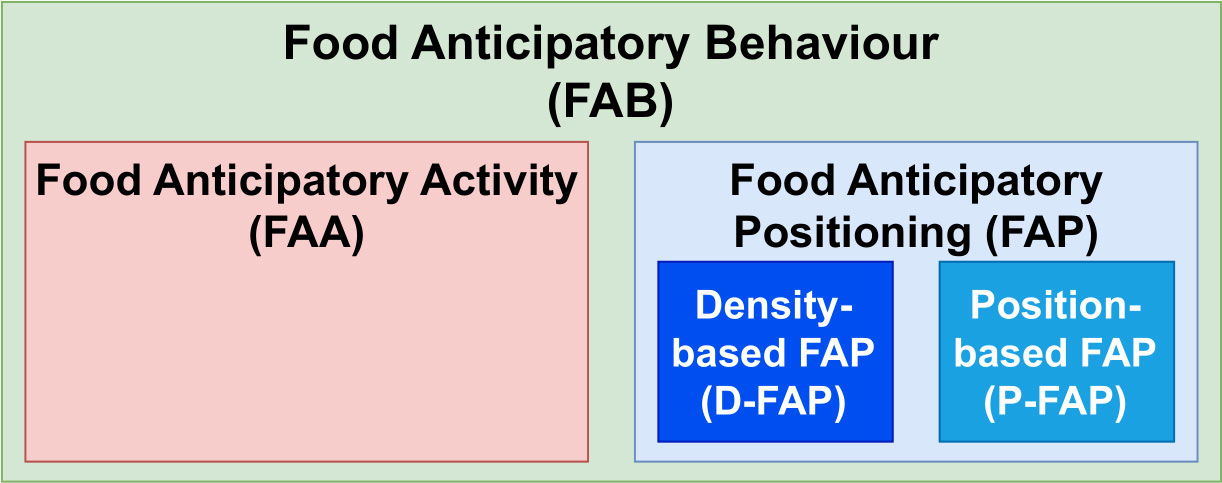
Figure 1 A unified terminology framework: food anticipatory behaviour (FAB) becomes the umbrella term encompassing food anticipatory activity (FAA) and food anticipatory positioning (FAP). FAA focuses solely on locomotor-driven methods; FAP splits into subcategories for density-based (D-FAP) or position-based (P-FAP) methods.

Material and methods

Receivers and transmitters

The vertical distribution, the swimming acceleration activity, and the temperature were measured by an array of three acoustic receivers (TBR700, Thelma Biotel Ltd.). The three receivers were submerged in the floating ring of the sea cage with the help of ropes to a depth of 2.5 m. The GPS positions in decimal degrees (N, E) formed a triangle: ($35.48011$, $24.112$), ($35.48006$, $24.11209$), and ($35.48$, $24.11196$). The acoustic tags used for implantation were low-power transmitters (ADT-LP7, Thelma Biotel Ltd.) with the following specifications from the producer: a diameter of 7.3 mm, a length of 23.2 mm, a weight in the air/water of 2.1 g/1.1 g (1.8 g measured weight in water in Georgopoulou et al., 2022), and a power output of 139 dB. The signal interval for depth is every 30–90 s (mean 60 s), and alternately, temperature or activity (mean 120 s). The transmitters measured depth through water pressure sensors with a resolution of 0.1 m. The temperature was measured with a temperature sensor, which has a resolution of 0.1 °C. The activity is measured in metres per square second using a three-axis accelerometer in each tag, which uses the root mean square over the three acceleration axes. The resolution was $0.013588 \text{m}/{\text{s}}^2$ with a range from 0 to $3.465 \text{m}/{\text{s}}^2$. The tags are calibrated such that the static component in acceleration readings (gravity and sensor offset) is subtracted from the total acceleration, resulting in animal acceleration readings. The transmitter tags were evenly distributed among the available frequencies (67, 69, and 71 kHz) to minimise the overlapping of signals. For details about the transmitter tag’s implantation into the peritoneal cavity of the fish, we refer to Georgopoulou et al. (2022).

One additional synchronization tag (R-HP16, Thelma Biotel Ltd.) was attached to one of the receivers for reference in order to use positioning calculations (PinPoint positioning system, Thelma Biotel Ltd., Norway, see Section "Expanding the dataset"). It has the following specifications: a diameter of 16 mm, a length of 70 mm, a weight in air/water of 29 g/14.9 g, a power output of 158 dB, and a frequency of 69 kHz.

Fish and tag implantation details

A whole E. seabass group was reared at the Hellenic Center of Marine Research (HCMR) in Crete, Greece. Fish originated from the Mesocosm hatchery of the AquaLabs, IMBBC of HCMR. Following larval rearing, pregrowing, and 120 days posthatching, juveniles with approximately 2 g mean weight were transferred to the pilot-scale cage farm of the institute (Souda Bay, Crete). The sea cage is made of a circular polyester cage with 40 m in diameter and 9 m in depth. The cage form is cylinder-shaped up to 8 m depth and has a cone that closes the cage at 9 m. More than 10,000 fish individuals were held in the sea cage in total.

This study continues the monitoring of the same 24 tagged E. seabass individuals that have been used in the study of Georgopoulou et al. (2022), where the implantation process for these fish is described in detail and also group swimming features postoperation are analysed. We present key points from the surgical procedure:

The fish of 32.17 ± 6.4 cm in length and 398.2 ± 73.3 g in weight, were caught from the sea cage and put into a tank of 10 ${\text{m}}^3$ volume at the HCMR facilities. The fish collection was random regarding sex. The sea cage to tank transfer was on 26 March 2021, the tag implantation on 26 April 2021, and the reintroduction into the sea cage was on 14 May 2021. In the tank period, the fish were fed once a day around 12:00. The tags were implanted in the peritoneal cavity of the fish, and the tag-to-body-weight ratio was under 2% (Jepsen et al., 2005). All fish survived the tag implantation treatment, and no additional invasive operations were conducted on the fish.

During the harvesting after the experiment, 22 of the tags could be recovered successfully.

Experimental design

The time window of the experiment was from 26 May 2021 at 00:00:00 to 06 June 2021 at 23:59:59 local time. The experiment started 1 month after the tag implantation, and the fish had 12 days of rehabilitation in the sea cage. The receivers were installed 2 days prior to the start of the experiment for testing purposes. The deactivation of the transmitters on 06 June 2021 marked the end of the data collection. The fish were manually fed once a day between 8:00 and 10:00. Commercial food pellets (Zoonomi S.A., Greece) were used for feeding. The feed quantity was approximately 35 kg per feeding. The feeding was done by hand, and the whole feeding process took around 30 min/day. First feed had to be transported to the sea cage, then spread manually by hand at the sea cage before leaving the vicinity. The time spent feeding the fish took 5–10 min.

For analysis, we split the sea cage into three depth segments: the upper water column ranged from 0 to 3 m depth, the middle water column ranged from 3 to 6 m depth, and the lower water column ranged from 6 to 9 m depth.

Data collection and processing

The process of data collection and processing was similar to Muñoz et al. (2020), since the same technology had been applied. Each data point in the dataset was a received signal with the parameters time, depth, and temperature/activity. A valid data point had been created if a signal sent by a transmitter is received by all three receivers with the same value, which also allows for GPS calculation. For the respective stages of refining the dataset, let n denote the number of valid data points from the transmitters in the dataset and k the number of total receiver data points ($k_1,k_2,k_3$ for the receivers respectively). Theoretically, the maximum number of valid transmitter data points is:

$$\begin{array}{c}1\times 60(\text{one signal per minute on average})\times 24\\ \times 12(\text{hours per day }\times \text{ experiment days})\\ \times 24(\text{number transmitters})=414,720(\text{valid data points})\end{array}$$

At the end of the experiment, the software ComPort (Thelma Biotel, v4.0.0) was used to download data (number of received signals in total: $1,199,017$) from the receivers and to filter the raw data from a technical standpoint. Only signals inside the experimental window were kept. Exclusions were also due to technical failures that caused random re- and deactivation of tags after the experiment. False detection (i.e., not listed IDs for transmitters) occurred due to the so-called collisions between acoustic signals sent by transmitters, and signals from the two missing tags were filtered, resulting in a total of $n=54,494$ data points. Horizontal position estimations were postcalculated by the manufacturer using triangulation based on the time differences of arrival from received signals (PinPoint positioning system, Thelma Biotel Ltd., Norway) by using the synchronization tag for reference. By the manufacturer’s procedure, a value called heatpoint deviation of optimal position (HDOP) was calculated, which shows the mean deviation between the calculated position and the known positions, thus a deviation error parameter. We refer to Muñoz et al. (2020) for more explanation. We applied multiple other filters to the dataset. One of them was the signal–noise ratio (SNR), which gives a quality measurement of the signal itself. The SNR bandwidth filter was $[20 \text{dB}, 50 \text{dB}]$ ($n=54,477$). The HDOP filter was set to $[0 \text{m},1.2 \text{m}]$ ($n=28,963$). We assumed fish temperature to be normally distributed for each individual (around the seawater temperature), resulting in only keeping data points with temperature values lying between −3 and 3 standard deviations (z-score). Finally, we only include data that have sensible depth values of 0 to 9 m ($n_{\text{final}}=28,952$). The time resolution of the left signal data from the 22 transmitters in this study showed a median of 6.18 min ($\text{IQR}=14.71-2.51$) in the experiment window. Status data from the receivers (i.e., temperature) ($k=61,008$) were not filtered except for the application of the experiment window ($k_{\text{final}}=5,184$, $k_1=k_2=k_3=1,728$). The time resolution of the receivers is exactly 10 min. Altogether, the postprocessed valid dataset has $n_{\text{final}}=28,952$ valid transmitter data points and the receiver dataset $k_{\text{final}}=5,184$ data points.

We could not identify stress events for the fish in the data, and the number of outliers ($n_{\text{outlier}}=11$) is more likely due to the collision of signals. Neither net cleaning nor harvesting was conducted at or in the vicinity of the sea cage during the experiment. The weather conditions were stable with sunny/partly sunny, warm, and rainless days.

Unconstrained dataset without validation

If we applied the same filtering mechanisms as described in Section "Data collection and processing" to the $384,868$ signals received during the experiment period, but without the constraints that the transmitter signals have to be received by all three receivers or that the received signals must have the same value, then we get a total of $m_{\text{final}}=378,391$ transmitter data points that do not contain horizontal positioning data (no triangulation). We did include this dataset, called the unconstrained dataset only in a comparative way with the valid dataset, as we cannot guarantee confidence in the data foundation. In marine studies where multiplying the receiver number in close proximity is not possible, for example, in the open sea with a wide receiver array where acoustic signals are picked up by one receiver at best, it is not applicable to use data redundancies to create a dataset in which higher confidence can be placed in. The unconstrained dataset will be also provided along with the valid dataset nonetheless for the sake of completeness.

Clustering with DBSCAN

Density-based spatial clustering of applications with noise (DBSCAN) (Ester et al., 1996) was used in the vertical-temporal analysis to identify high-density areas, meaning a high number of transmitter signals in the same vertical area during short time periods. The method was used with the standard parameter ϵ=0.5 and a chosen number of minimal samples of 300. In sea cage terms, the choice of ε translates to the measure that, for example, two points closer than 0.5m depth distance with no time difference or points with half an hour time lag and no depth difference will have the Euclidean distance of 0.5 and therefore be considered neighbours. The parameter minimal samples describe the minimal number of points required in the ϵ-neighbourhood of a point for it to be a so-called core point. The point itself is always in its own neighbourhood. The choice of minimal samples was naively put together based on the number of signals in the dataset. Dividing $n_{\text{final}}=28,952$ up across 24 h and nine 1-m-depth columns, we would expect $(28,952/24)/9\approx 134$ data points per hour per 1m water column if data points were evenly distributed. In total, 300 data points were chosen as a threshold for a density cluster. The resulting clusters are mutually intra-density-connected, and isolated points were labelled as noise points. The results were mathematically deterministic (Schubert et al., 2017), meaning that execution of the code without changes to the published data will give the same clustering result as presented. The implementation from the Python package scikit-learn (Pedregosa et al., 2011) was used. However, we precalculated the Euclidean distances ourselves prior to the execution of the library code in order to account for the periodic nature of the hours of the day. For example, two data points sharing the same depth value but having the timestamps 00:01 and 23:59, respectively, should naturally have a time distance of 2 min for clustering, but that value would, by standard application of the Euclidean distance, be 23 and 58 min.

Sunrise and sunset times

Sunrise and sunset were not fixed for the duration of the experiment. A 24-h day was therefore split into night, civil twilight, nautical twilight, astronomical twilight, and day, with their respective times extracted from Geoscience Australia (2021) to adjust for photoperiod-related behaviour.

Quantification and statistical analysis

All statistical analyses were conducted using Python (v.3.9 and several packages) as well as R (v.4.2). On the unconstrained transmitter dataset, values were weighted after the number of receivers that caught the signal with that specific value. In all statistical analyses, the data were mean-binned (or count-binned) over 20-min periods, resulting in statistical units like mean acceleration, mean temperature, and mean depth per 20 min. Permutation tests between the different water columns with respect to time, with the sample mean difference as test statistics, were used. Kolmogorov–Smirnov goodness-of-fit tests were used between the two kinds of temperature data (transmitter valid, receivers) and between the activity data from the valid transmitter data and the depth data to find out if the data samples were originating from the same underlying distribution. The Pearson correlation coefficient had been calculated between the receiver temperature data and the fish activity data. A Kruskal–Wallis test was performed on the diving behaviour to test if the fish followed a specific hourly diving pattern. A p-value of $p<0.05$ was considered significant.

We followed the two typical conditions of activity peak and peak persistence for fish (Sánchez-Vázquez and Madrid, 2001) and chose a similar strategy as Azzaydi et al. (2007) did in their study on E. seabass, where the fish were under natural conditions in an outdoor laboratory. We note that the fish in Azzaydi et al. (2007) had only around a third of the weight as the ones in our study, but since measuring FAA is using the fish themselves as a baseline, the measurements should only differ in the absolute values. Instead of defining FAA as a 50% increase in activity against a baseline and calculating the FAA duration as the time the activity lasted, we set up the following for locomotor-activity-based FAA:

1. The activity level must be over the 0.5 quantile for the respective 24-h day.

2. The increased level of activity persists over six 20-min periods (120 min).

If both criteria were fulfilled, we noted that we were able to detect FAA. This setup has the advantage that it is more data-driven; we do not need to establish a baseline at certain times whose choice could be operator-biased and thereby decrease manual tuning.

With 120 min as the minimum required time window, we expect that this will always be fulfilled by the feeding activity; therefore, the minimum FAA time window of 0 min is reachable. This ensures that the algorithm is falsifiable in the FAA detection. The algorithmically obtained high-activity windows were reduced to FAA time windows by only keeping high-activity windows before 8:00 (when the feeding period starts). For later comparison between the different FAB approaches, we considered FAA on the whole activity dataset for the hours of the day and without the algorithmic constraint that the high-activity time windows are cut off at 8:00. Additionally, the mean-binning was set to 5-min periods due to the abundance of data points when using the hours of the day. A seasonal decomposition was calculated on the activity data throughout the hours of the day.

Pseudo-random interval shuffling

A pseudo-random baseline for the time was created by the pseudo-random interval shuffling (PIS) procedure, which is similar to the inter-spike interval (ISI) shuffling procedure (Vinepinsky et al., 2020) to dismantle information (i.e., temporal) between intervals. Instead of identifying spike trains, all 20-min resamplings (by mean or count) were shuffled by pseudo-random permutation. The time of day distribution for each water column was Chi-square tested against multiple ($n=10,000$) PIS baselines. The resulting p-values were then combined by Fisher’s method.

Results

Diving behaviour

Figure 2 visualizes the vertical fish distribution in the water column using a binning into the time of day (day, various twilights, and night). Figures 3A, B shows the vertical fish distribution created using 2-h periods for binning, from sunrise to sunset.

FIGURE 2

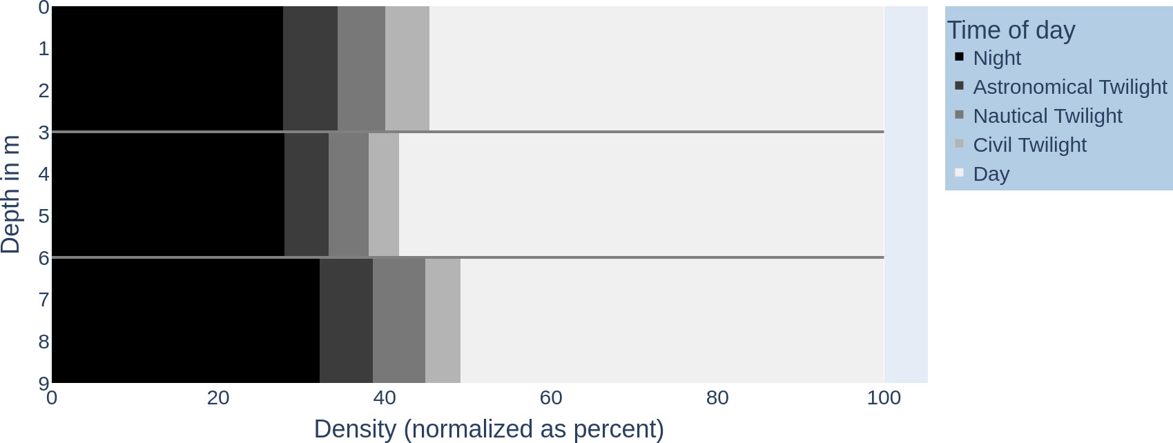
Figure 2 Fish distribution in the water column over daytime intervals: x-axis—density of fish (normalized as per cent) (0–100); y-axis—depth in metres (0–9 m). The time intervals are shaded accordingly: night (black), astronomical twilight (dark grey), nautical twilight (grey), civil twilight (light grey), and day (white).

FIGURE 3

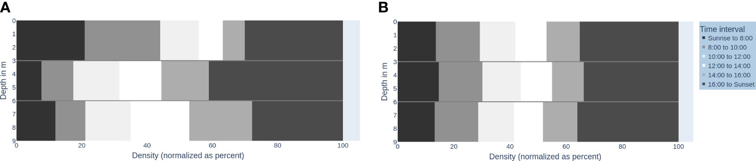
Figure 3 Fish distribution in the water column over daytime intervals (A) and a time-shuffled version (B). The x-axis: Density of fish (normalized as percent) (0-100), y-axis: Depth in m (0-9m). The time intervals are shaded accordingly: Sunrise to 8:00 (very dark grey, 8:00-10:00 (dark grey), 10:00-12:00 (very light grey), 12:00-14:00 (white), 14:00-16:00 (light grey), 16:00 to sunset (darker grey).

When counting the different twilight types (official, nautical, astronomical) as part of the time of day “day”, we observe that the day proportion of the 24-h day across the water columns is rather uniform with 70.71% (± 4.1%) (see Figure 2). On the other hand, the vertical distribution of fish individuals is not uniform; individuals have different preferences in depth (see Figure 4; in total, the median was 3.3 with IQR = 5 − 1.6).

FIGURE 4

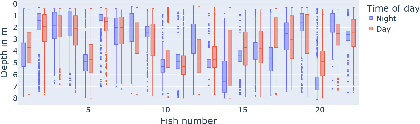
Figure 4 The preferred vertical water column position of the tagged fish individuals split by day (red) and night (blue). The x-axis describes the fish number identifier, and the y-axis is the depth in metres (reversed axis for visualization).

A Kruskal–Wallis test was conducted to examine the differences in the hourly diving pattern, which resulted in significant differences (${\chi }^2=288.24$, $df=23$, $p<0.05$). On a group level, the diel vertical movement included that fish are near the surface longer and denser in the morning compared to a shorter evening spike (see Figure 5). Generally, fish appear to avoid the surface between 12:00 and 17:00, and at night, the whole water column is used (see Figure 5).

FIGURE 5

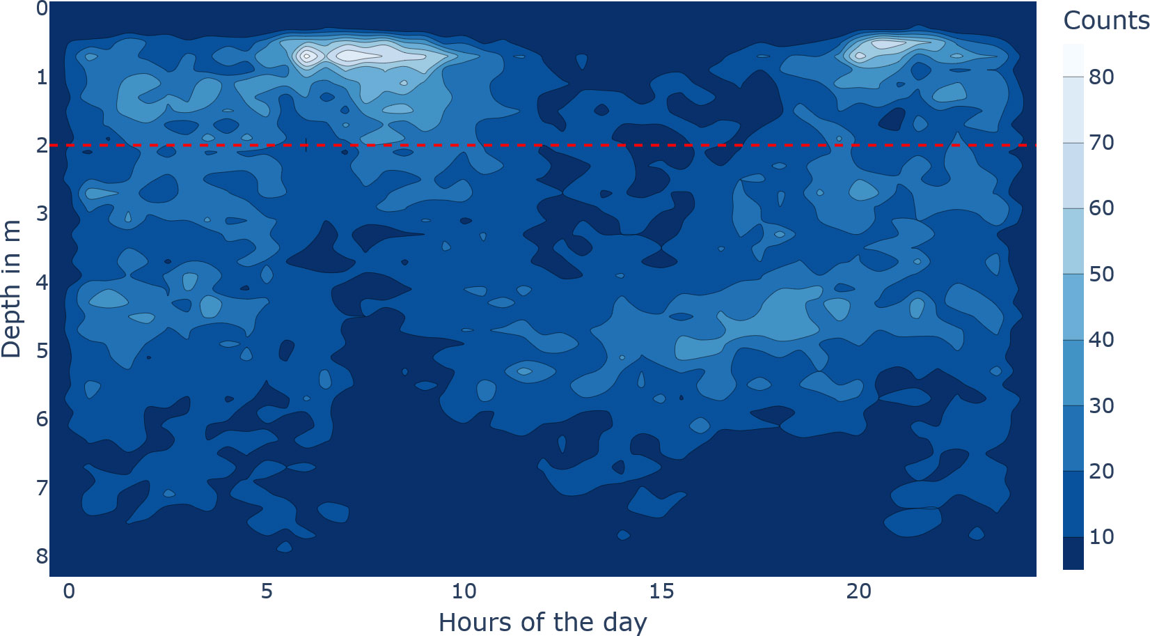
Figure 5 Diving behaviour of the tagged fish. The x-axis describes the hours of the day, and the y-axis describes the depth in metres. The brighter the colour, the denser the fish were at that time-depth bin. The horizontal dashed red line at 2 m depth emphasizes the very upper water column.

Activity and temperature

The average activity levels followed a 24-h period with the highest peak for the respective day consistently being between 6:00 and 10:00 (see Figure 6 for activity levels, dark blue line). The average activity of the time series was $0.77 \text{m}/{\text{s}}^2\pm 0.41$, ranging from 0.095 to $3.465 \text{m}/{\text{s}}^2$. Under the seasonal decomposition (see Figure 7), stability (variance of mean) was under 0.1 and lumpiness (variance of variance) was under 0.01. The seasonal decomposition leads to a trend strength of 0.9 and a seasonality strength of 0.35. The spectral entropy value of the activity time series is 0.37.

FIGURE 6

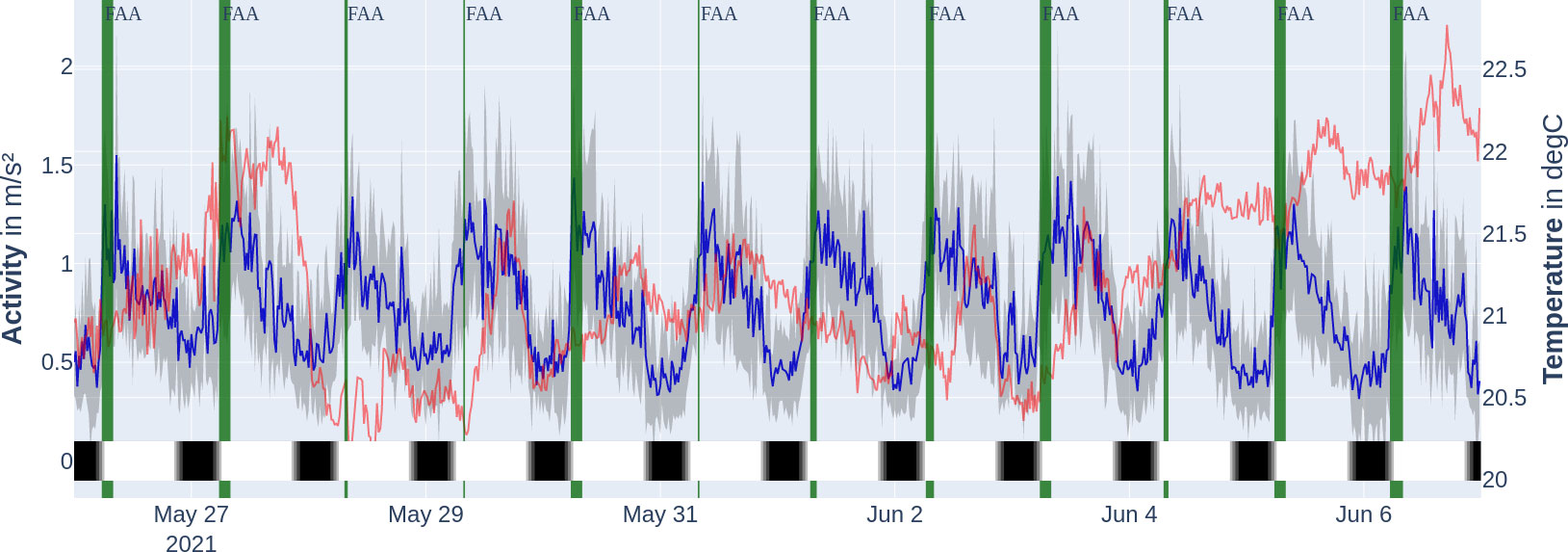
Figure 6 Mean acceleration activity profile of tagged fish (dark blue, with 1 SD in grey) over the temperature of tagged fish (faint red) during the experiment period. Locomotor-activity-based FAA window (cut off at 8:00 when feeding window starts) marked with vertical bars (dark green). The thicker the vertical bar, the longer the FAA was observed. The bottom colour bar encodes the time of day on that specific day: night (black), astronomical twilight (dark grey), nautical twilight (grey), civil twilight (light grey), and day (white). Note that the twilight zones are hardly visible.

FIGURE 7

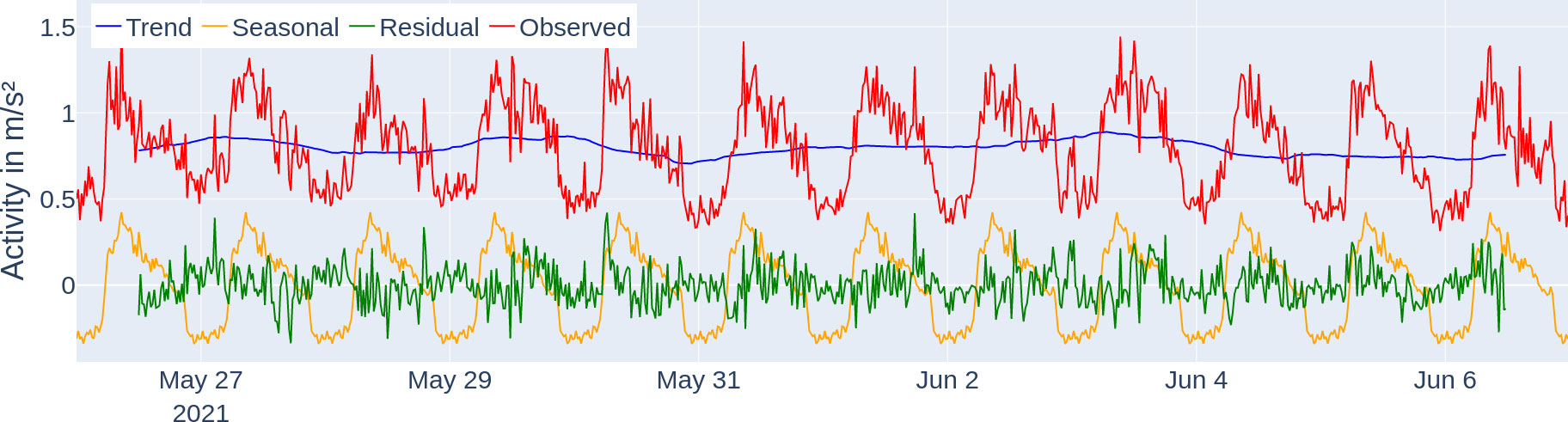
Figure 7 Seasonal decomposition of the activity profile of tagged fish. The trend (blue) component describes the general direction of the activity, the seasonal (yellow) component shows the daily repeating pattern, and the residual (green) component describes the unexplained fluctuations after removing the trend and seasonal component. The observed activity data (red) can be additively reconstructed from the three components (trend, seasonal, and residual).

There was a significant difference between the temperature datasets. The temperature data from the transmitters were sampled from populations with a different distribution than the temperature data from the receivers after Kolmogorov–Smirnov (goodness-of-fit test, $p<0.05$). No significant correlation ($p\ge 0.05$, Pearson correlation coefficient) was found between the alternating transmitter temperature and fish activity data on a 20-min group scale (see Figure 6 for visualisation of transmitter temperature and fish activity data). A noncorrelation was also found between the receiver temperature data and the fish activity data observed using the Pearson correlation coefficient ($p\ge 0.05$). It thus remained inconclusive whether the temperature span of $20.92\pm 0.59 °\text{C}$ (receiver temperature measurements) was a factor influencing the acceleration activity.

Fish anticipatory behaviour

Food anticipatory activity

We were able to extract exactly one locomotor-driven FAA window per day which last longer than 120 min (per the description of our detection method in the Section "Quantification and statistical analysis" more windows were possible). Since the time windows all reach into the feeding period, they are marked as FAA time windows from their beginning up to the feeding period, which starts at 8:00 (see Figure 6). The actual daily starting times for the locomotor-activity-based FAA based on the method explained in the Section "Quantification and statistical analysis" are stated in the Supplementary material (Supplementary Table S1) and correspond to the width of the vertical dark green bars in Figure 6. Therefore, FAA activity starts on average at 06:21 ± 00:52. The peak in seasonal (periodic) influence is at 8:40, and lowest at 22:40, respectively (see Figure 7, yellow line). When using the FAA detection method as described in the Section "Quantification and statistical analysis" for all activity data on the hours of the day with a 5-min binning, we report that the only high-activity window is the FAA window starting at 5:45.

A position-based approach

The accumulation of signals in the upper water column from sunrise to 10:00 (see Figure 3A, very dark grey and dark grey top sections) makes up 51.71% of the total signals in the upper water column. This pattern is significantly not random against shuffled permutations (PIS) ($p<0.05$ for each water column). Patternless distributions would look like the illustration in Figure 3B. The pattern can differ across days, but all daily patterns are significantly not random in time against shuffled permutations (PIS) ($p<0.05$ for each water column). Thereby, we find P-FAP time periods for the intervals between sunrise (5:48–5:50, depending on the day) and 8:00 (start of feeding).

A density-based approach

The DBSCAN clustering results (see Figure 8) show two spatiotemporal clusters. Cluster 0 spreading from 1.7 to 0 m depth highlights the positioning of the fish in the upper very top of the water column prefeeding and during feeding. Cluster 0: the density distribution (see Figure 9) shows the relevance of the clusters (highest probability density with 2.6%). This cluster 0 is the biggest cluster found through the DBSCAN method, and it precedes the earliest FAA time window concluded in Section "Food anticipatory activity" with a D-FAP time window from 5:08 to 8:00 (5:08 to 9:48 total time window). There is also cluster 1 near the surface, which ranges from 19:31 to 21:26 time-wise and from 0 to 1.3m in depth. It is even denser than cluster 0 (highest probability density at 4.15%).

FIGURE 8

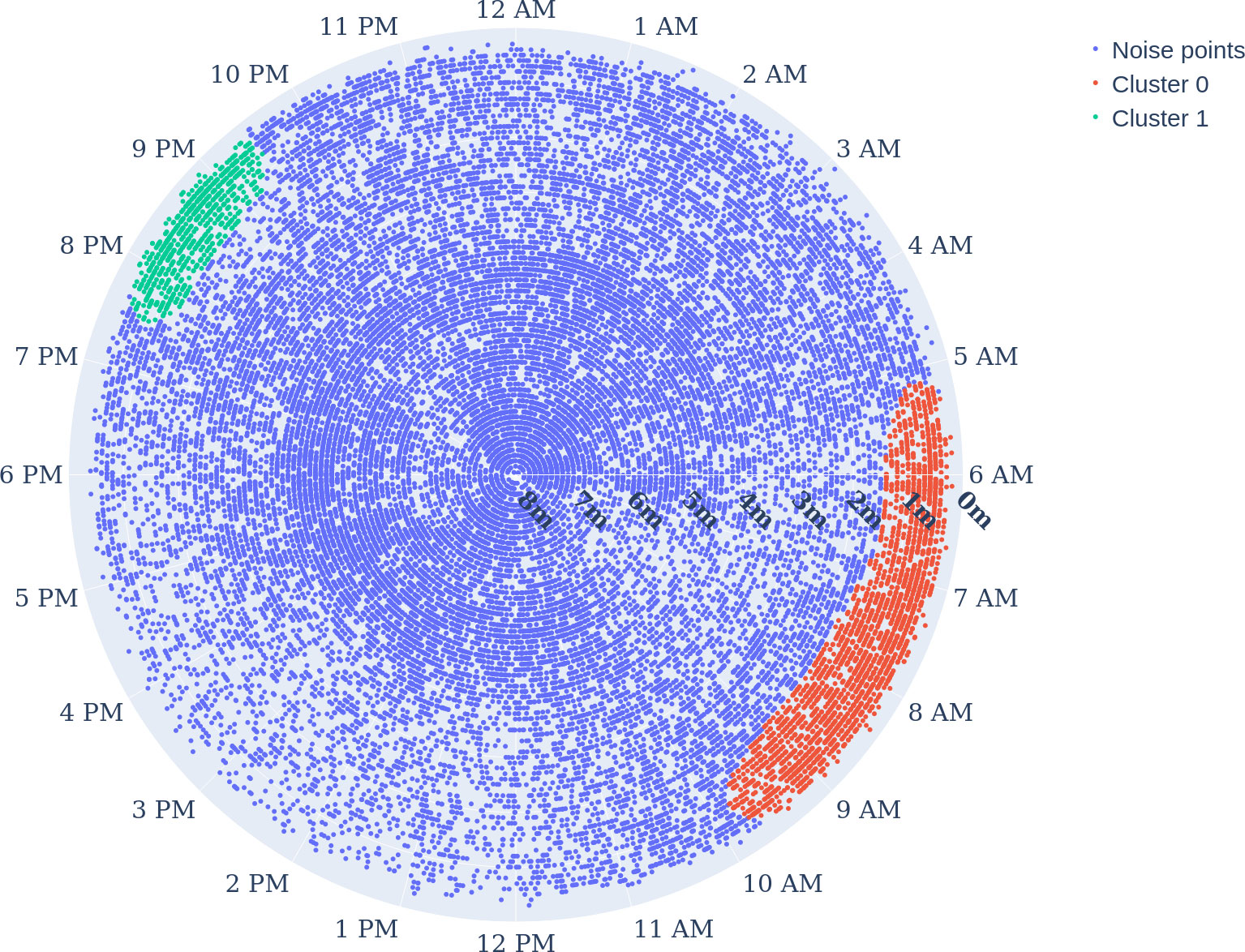
Figure 8 Clustering the time-depth data points of the whole experiment period: radial axis describes the depth, and the angular axis represents the hour of the day. Hyperparametres were ε=0.5, and the minimum sample size was 300. Clusters 0 in red and 1 in green show the dense positioning of E. seabass close to the surface, and noise (no cluster) in blue.

FIGURE 9

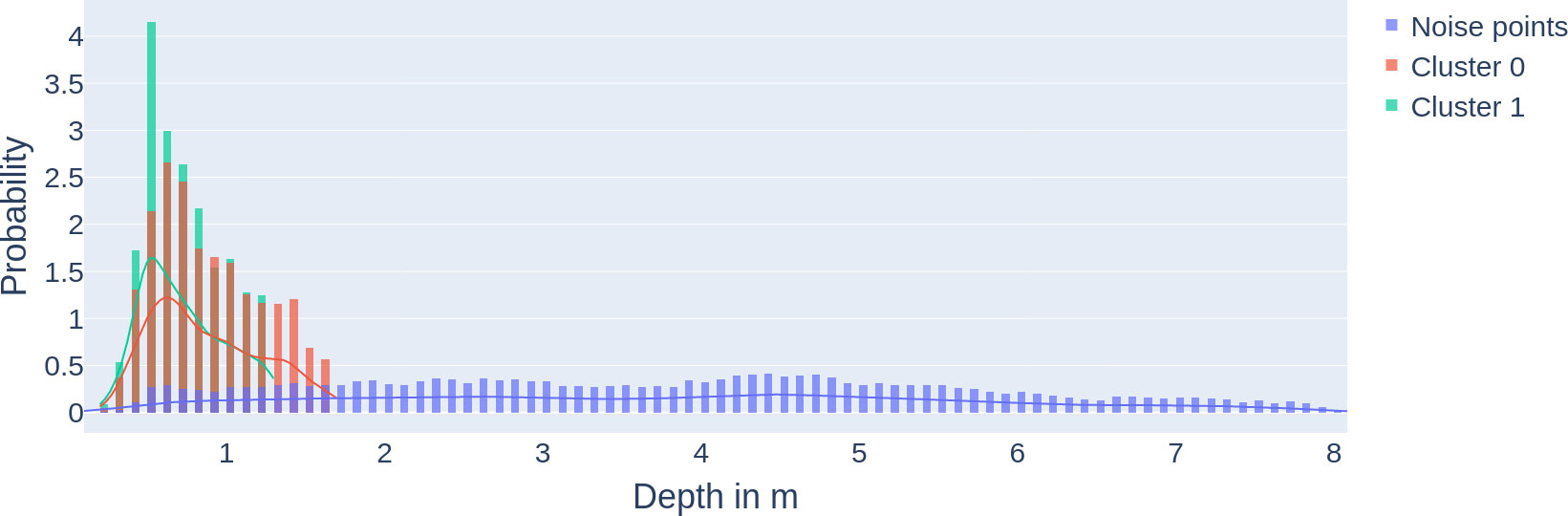
Figure 9 Density of fish clusters close to the surface: multilayer probability density function (and histograms) of clusters 0 and 1 and the noise points from Figure 8. The x-axis describes the depth, and the y-axis describes the probability.

Discussion

Comparison of FAB approaches

This is the first study to our knowledge that used an unsupervised density-based approach to measure near-surface positioning in conjunction with FAA in E. seabass and finfish in general.

We were able to extract not only morning anticipatory behaviour, which precedes the FAA time window, but also a dense cluster in the evening (see cluster 1 in Figure 8). This is an extension of what classical FAA can provide; depending on the hours of the day, FAA could neither be observed as early as D-FAP nor in the evening (see Figure 10). We hypothesize that the actual positioning near the surface precedes possible recordings of increased activity (over 0.5 quantile), and therefore classical locomotor-activity-based FAA is not detectable, even though it should be measured as an anticipatory behaviour. For the evening density cluster, we hypothesise that the accumulation in the surface area is part of the natural behaviour of E. seabass to prefer dim light to forage (Bégout Anras, 1995). While the cluster is technically not food-entrained FAB, we marked it as D-FAP, which was not rewarded with food. Higher surface temperature as a reason is unlikely due to the stable environmental conditions and small range of temperature during the experimental period (see Figure 6).

FIGURE 10

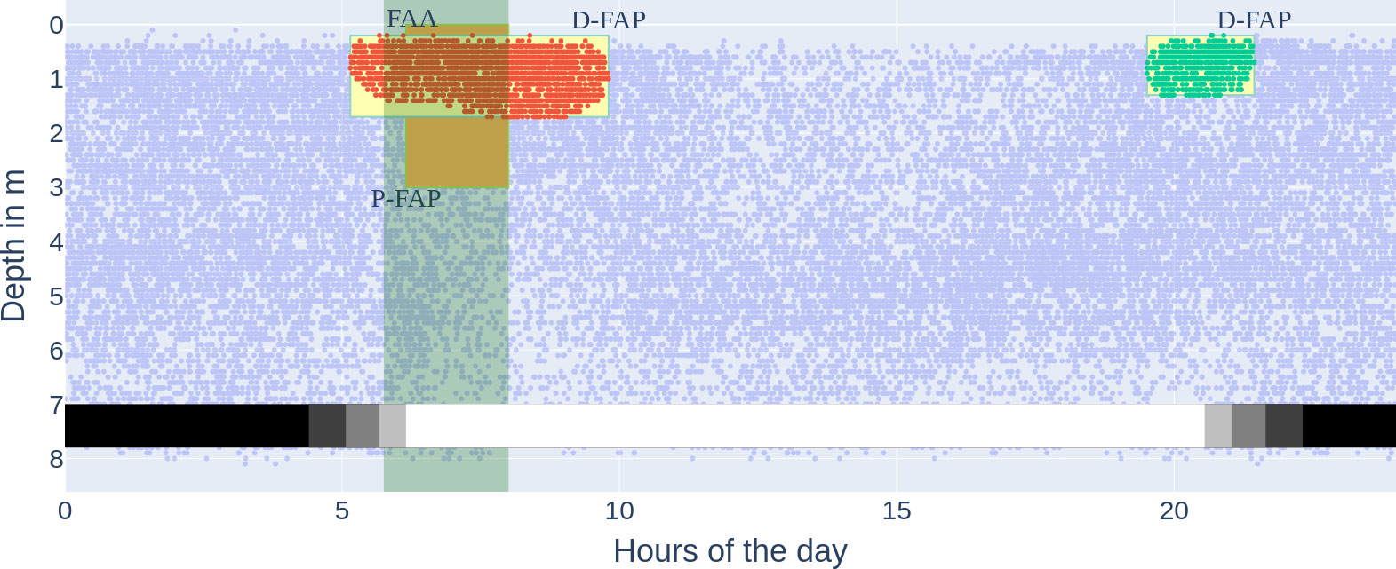
Figure 10 All three methods for food anticipatory behaviour on the accumulated data in the experimental period, marked by time and depth if applicable. FAA, locomotor-activity-based FAA (light green vertical bar); P-FAP, position-based Food Anticipatory Positioning (orange box); D-FAP, density-based food anticipatory positioning (yellow boxes). The x-axis describes the hour of the day, and the y-axis describes the depth in metres. Each dot is one (time, depth) datapoint from the tagged fish. The FAA time window was calculated according to the Quantification and statistical analysis. The two clusters (red and green) are the same clusters as in Figure 8 (the red cluster not cut off by feeding start at 8:00). The faint blue dots are the same noise points as in Figure 8.

The bigger size of the morning cluster (cluster 0) is most likely also the result of a compound effect between the natural behaviour and the D-FAP since there is a positive relationship between FAA duration and dawn/dusk (Azzaydi et al., 2007).

These findings indicate that D-FAP can provide insight into not only the entrained food anticipation in the morning but also other behavioural patterns, such as foraging behaviour in E. seabass (Paspatis et al., 1999).

Comparing D-FAP and P-FAP, we conclude that D-FAP is favourable due to two main reasons. Firstly, the data basis for D-FAP is the original data points themselves with their respective timestamps. Thereby, the start of the detected D-FAP can be accurately given by the earliest occurring datapoint in a dense cluster, while for P-FAP, pre-defined time intervals limit the possible choices when FAB is detected. Secondly, the choice of time slot duration underlies human bias (we expected only FAB in the morning) and does not, for example, cover a chance to detect the evening behaviour. The presented P-FAP detection method therefore only allows for a quick analysis of FAB in the morning, but it is neither precise nor does it detect all fish activity (see Figure 10).

Comparing detected P-FAP and FAA, the P-FAP method suffers from the same problems as FAA in comparison to D-FAP. Both do not detect evening FAB activity. Additionally, P-FAP is more limited than FAA regarding the starting time for FAB, which makes it only a good proxy for FAA when the time intervals are preset properly. In our results, P-FAP is detected after FAA has been detected. The silver lining for P-FAP is that it is a method that can be implemented by other means, too, especially cameras, since counting the appearance of fish is the key factor in this method and not the density. Adaptations of proxies such as the “fish index” (Folkedal et al., 2012b) could be used to implement this FAB detection method, but the decision on the temporal resolution remains a human operator task.

All in all, the detection differences in FAA and especially D-FAP exemplify the main research message we want to convey: being active is not necessarily the same thing as being somewhere specifically. Especially not for fish, who can inherently use all three space dimensions to position themselves. The opposite is also true: being somewhere specifically does not necessarily mean activity. Therefore, considering multiple viewpoints on such a sensitive welfare indicator can be beneficial to accessing a more complete picture of FAB.

Food anticipatory behaviour as an umbrella term

So far, FAA has been widely used as an umbrella term for all expressions of food anticipation and can lead to mislabelling or misunderstanding of the actual underlying behaviour. While most previous studies have focused on FAA as a locomotor-driven measure, we present a dissection of anticipatory behaviours to include more specific terminology and suggest the usage of the umbrella term food anticipatory behaviour together with the subcategories FAA and FAP (further divided into P-FAP and D-FAP) (see Figure 1).

There is previous work that hints that using only FAA for all kinds of food anticipation may be outdated, and the authors had to deal with the underlying terminology problem. Some studies based on the position or density of the fish are already addressing the naming issue by introducing the term “food anticipatory behaviour” and are not referring to FAA as a term at all when analysing anticipatory behaviour (Folkedal et al., 2012a, b). “Food anticipatory activity behaviour” (Luby et al., 2012) in mice consisted of tracking high-intensity activity using cameras, which is a study on FAA after the presented terminology. In the end, there is also work abbreviating food anticipatory behaviour and food anticipatory activity both to FAA (Acosta-Galvan et al., 2011). These studies serve solely to support the point that there is already a movement away from the term “food anticipatory activity” for all kinds of food anticipation.

Areas of exploration

An area of exploration appears through the separation of FAB into FAA and FAP, i.e., the connection between FAP and Time-Place Learning (TPL) for finding food. TPL in general refers to animals’ ability to remember several events that vary spatiotemporally (Mulder et al., 2013), which is basically what P-FAP is when the memory is about food. Using the positioning of the fish to measure TPL (Reebs, 1993; Reebs, 1996) could have been categorized as a form of P-FAP if the experiments were set up differently. It could be possible that the evening cluster (cluster 1) is an exhibition of the more general TPL and is unrelated to (pre)feeding behaviour, but further experiments are needed to confirm this. Further research is generally needed to unravel the relationship between FAP, which only measures anticipation of food in a certain position after entrainment, and TPL, which also measures avoidance.

An already explored area of research is the link between FAB and appetite and feed uptake. In general, digestive and metabolic processes prior to feeding allow the processing of food in bulk quantities (Stephan, 2002; Strubbe and van Dijk, 2002) if the underlying food-entrainable oscillator for FAA is trained toward the feeding schedule. Indication of this in fish is also found, as in Gilannejad et al. (2021), where the digestive tract exhibits preparatory activity prior to daily feeding, as shown in the higher expression of genes involved in protein digestion for Senegalese sole (Solea senegalensis). A better understanding of the pre-feeding behaviour, like with D-FAP, may be a useful tool to track behavioural activities to align appetite and the exhibited FAB to maximize nutritional value and thereby increase welfare by feeding after appetite. Further studying the link between FAB and the digestive system may prove useful for farmed fish, as it adds another component to understanding FAB also on a nutritional level.

Lastly, research efforts focussed on E. seabass could reveal possible connections between FAB to the known capabilities of E. seabass to shift between diurnal and nocturnal feeding patterns (Azzaydi et al., 2000). For example, it would be interesting to explore if anticipation behaviour in the morning and evening can be used to facilitate the shift between feeding patterns.

Expanding the dataset

Using the 20-min resolved activity data, FAA starting points differ between the days. We show that using the unconstrained dataset results in more evenly long-lasting FAA time windows, and the starting time distribution is less volatile than for the valid dataset (see Supplementary Figure S1). We argue that this is due to the larger number of signals compared to the valid dataset, which therefore smooths the activity curve over the 20-min periods. We do not encourage the use of the unconstrained dataset to draw conclusions since the underlying population for the two datasets is significantly different (Kolmogorov–Smirnov goodness-of-fit test).

Future possibilities of acoustic telemetry

Individual acoustic telemetry provided detail-rich information about individual E. seabass, and also gave the possibility to analyse the group’s behaviour. Data had to be aggregated over time and individuals to make up for the lost data in practice, but being able to resolve time in 20 min is arguably fine enough for automatic feeding systems. The time resolution for a 24-h cycle could even be increased to 5-min intervals. The knowledge gained from telemetry tags has the potential to be used to qualify other noninvasive observation methods such as hydroacoustics or camera systems, as described in Føre et al. (2018a). Individual tagging also reveals knowledge about the fish individuals, even though this was not the focus of this study. It remains debatable how much acoustic telemetry can be used in the industry outside of marine research since acoustic tags and the receiver array are costly, and tags have to be found in the slaughter process to avoid foreign materials in the end product. Additionally, minutely time resolution remains a problem: although we theoretically could have received 414,720 valid signals (as discussed in Section "Data collection and processing"), the number of usable data points was 28,952 ($\approx 7\%$) in the valid dataset, which translates to time gaps in the data collection and shows that the usage of acoustic telemetry has its limitations. Another underlying problem of this technology will always be that only a part of the fish group is reflected in the acquired data, and their behaviour on a small group level may not be in sync with the behaviour on a sea cage group level. Though we support following this line of technology, acoustic telemetry tags like ours still require an invasive operation. Though the number of individuals chosen was small, technological advancements in tagging tools (i.e., smaller/external transmitters) are needed to further ensure the welfare of the tagged fish.

Vertical distribution

Schurmann et al. (1998) established a reference for the vertical diurnal rhythm of E. seabass in tanks, and Quayle et al. (2009) for free-roaming seabass. We add to this with the sea cage as an environment and Figure 5 as a reference for the diving behaviour of farmed E. seabass with daily morning feeding.

Limitations

There are several limitations to this study. Firstly, there is only a short history of studies on FAP and especially D-FAP, such that any generalization of our results should be interpreted with caution. Secondly, there were time constraints in the data collection, which resulted in a short experimental period. Another limitation is that the presented method with DBSCAN for D-FAP needs hyperparameter tuning from an expert, and the data amount needs to be sufficiently high. However, we anticipate that more sophisticated models will make human experts unnecessary for hyperparameter tuning. As hinted at in Supplementary Figure S4, only looking at singular days does not lead to interpretable results. Furthermore, all presented methods do not consider individual fish but only the group behaviour of the tagged fish. Knowledge transfer from our results to single individual fish is thereby discouraged. Further research is needed in order to investigate the application of position- and density-based approaches, which may lead to more accurate quantification of FAB in E. seabass, but also farmed fish in general, since a feeding direction is usually given in aquaculture settings, whether tanks or sea cages.

One underlying assumption in this work was that acceleration activity is a proxy for activities like locomotor-driven FAA and feeding activity, not just for gilthead seabream (Palstra et al., 2021), but also for E. seabass. Additional factors like photoperiod, feeding times, and feeding mode play a major role in fish activity, which have been analysed separately or in combination in other studies (Sánchez-Vázquez et al., 1995; Azzaydi et al., 1998; Sarà et al., 2010; Lanteri et al., 2016). Together with the fact that foraging behaviour and thereby being close to the surface is linked to twilight times (Boujard et al., 1996; Paspatis et al., 1999), all morning and evening FAB are likely to be partially due to evolutionary reasons that cannot be separated.

Conclusion

Further digitization is an important keystone to move toward data-driven decision processes, and with regard to feeding, the decision on time, the period, and the volume is the core of fish feeding.

Collectively, our results show that food anticipation in E. seabass (and also other fish species through literature) has more facets than classical locomotor-driven FAA, and future anticipatory behaviour classification in fish may consider the use of a more detailed framework. More in-depth research is needed to uncover the specific temporal relationships between FAP and FAA as well as FAP and TPL. Furthermore, methods of reliably tracking daily FAP have to be developed. Acquiring accurate FAB knowledge by combining FAA with FAP may have the potential to support fish farmers in shifting feeding regimes with higher precision, which can improve both the economic value of the fish and the welfare aspects.

Data availability statement

The unconstrained dataset and the valid dataset for this study are published under the Creative Commons CC-BY 4.0 license with the DOI: 10.5281/zenodo.7900273. The Python code is published under the Apache License 2.0 and the latest code release has the DOI: 10.5281/zenodo.7977064. With the Python code, the main statistical analysis and all Figures except Figure 1 can be reproduced. Figures 2, 3, 6 based on the unconstrained dataset can also be reproduced by the code and are found in the Supplementary Material.

Ethics statement

The HCMR aquaculture facilities are certified by the national veterinary authority (code GR94FISH0001) and licensed for operations of breeding and experimentation with fish issued by Region of Crete, General Directorate of Agricultural & Veterinary no. 3989/01.03.2017 (approval codes EL91-BIObr-03 and EL91-BIOexp-04). The experimental protocol for fish implantation was reviewed and approved by the Ethics Committee of the IMBBC and the relevant veterinary authorities (Ref Number 32257 09-02-2021) in accordance with legal regulations (EU Directive 2010/63).

Author contributions

I-HC: data curation, formal analysis, methodology, statistics, Python coding, open data management, and writing the original manuscript. DG: data generation, statistics, data curation, R-coding, methodology, interpretation of data, and internal review. LE: acquiring funding, conceptualization, experiment planning, interpretation of data, and internal review. DV: data generation and hardware handling. PL: supervision of data analysis and statistics, interpretation, and internal review. NP: acquiring funding, conceptualization, experiment planning, data generation, facility management, interpretation of data, and internal review. All authors contributed to the article and approved the submitted version.

Funding

This work was funded by the iFishIENCi project and has received funding from the European Union’s Horizon 2020 research and innovation program under grant agreement No. 818036 and the Norwegian Research Council, Project number 323300.

Conflict of interest

The authors declare that the research was conducted in the absence of any commercial or financial relationships that could be construed as a potential conflict of interest.

Publisher’s note

All claims expressed in this article are solely those of the authors and do not necessarily represent those of their affiliated organizations, or those of the publisher, the editors and the reviewers. Any product that may be evaluated in this article, or claim that may be made by its manufacturer, is not guaranteed or endorsed by the publisher.

Supplementary material

The Supplementary Material for this article can be found online at: https://www.frontiersin.org/articles/10.3389/fmars.2023.1168953/full#supplementary-material

References

Acosta-Galvan G., Yi C.-X., van der Vliet J., Jhamandas J. H., Panula P., Angeles-Castellanos M., et al. (2011). Interaction between hypothalamic dorsomedial nucleus and the suprachiasmatic nucleus determines intensity of food anticipatory behavior. Proc. Natl. Acad. Sci. 108, 5813–5818. doi: 10.1073/pnas.1015551108

CrossRef Full Text | Google Scholar

Alfonso S., Zupa W., Spedicato M. T., Lembo G., Carbonara P. (2022). Using telemetry sensors mapping the energetic costs in European Sea bass (Dicentrarchus labrax), as a tool for welfare remote monitoring in aquaculture. Front. Anim. Sci. 3. doi: 10.3389/fanim.2022.885850

CrossRef Full Text | Google Scholar

Arechavala-Lopez P., Uglem I., Fernandez-Jover D., Bayle-Sempere J. T., Sanchez-Jerez P. (2011). Immediate post-escape behaviour of farmed seabass (Dicentrarchus labrax l.) in the Mediterranean Sea. J. Appl. Ichthyol. 27, 1375–1378. doi: 10.1111/j.1439-0426.2011.01786.x

CrossRef Full Text | Google Scholar

Azzaydi M., Madrid J. A., Zamora S., Sánchez-Vázquez F. J., Martinez F. J. (1998). Effect of three feeding strategies (automatic, ad libitum demand-feeding and time-restricted demand-feeding) on feeding rhythms and growth in European sea bass (Dicentrarchus labrax l.). Aquaculture 163, 285–296. doi: 10.1016/s0044-8486(98)00238-5

CrossRef Full Text | Google Scholar

Azzaydi M., Martinez F., Zamora S., Sánchez-Vázquez F., Madrid J. (2000). The influence of nocturnal vs. diurnal feeding under winter conditions on growth and feed conversion of european sea bass (dicentrarchus labrax, l.). Aquaculture 182, 329–338. doi: 10.1016/S0044-8486(99)00276-8

CrossRef Full Text | Google Scholar

Azzaydi M., Rubio V. C., Lopez F. J. M., Sánchez-Vázquez F. J., Zamora S., Madrid J. A. (2007). Effect of restricted feeding schedule on seasonal shifting of daily demand-feeding pattern and food anticipatory activity in European Sea bass (Dicentrarchus labrax l.). Chronobiol. Int. 24, 859–874. doi: 10.1080/07420520701658399

PubMed Abstract | CrossRef Full Text | Google Scholar

Barreto M. O., Rey Planellas S., Yang Y., Phillips C., Descovich K. (2022). Emerging indicators of fish welfare in aquaculture. Rev. Aquacul. 14, 343–361. doi: 10.1111/raq.12601

CrossRef Full Text | Google Scholar

Bégout Anras M. (1995). Demand-feeding behaviour of sea bass kept in ponds: diel and seasonal patterns, and influences of environmental factors. Aquacul. Int. 3, 186–195. doi: 10.1007/BF00118100

CrossRef Full Text | Google Scholar

Bégout Anras M., Covés D., Dutto G., Laffargue P., Lagardère F. (2003). Tagging juvenile seabass and sole with telemetry transmitters: medium-term effects on growth. ICES J. Mar. Sci. 60, 1328–1334. doi: 10.1016/S1054-3139(03)00135-8

CrossRef Full Text | Google Scholar

Boujard T., Jourdan M., Kentouri M., Divanach P. (1996). Diel feeding activity and the effect of time-restricted self-feeding on growth and feed conversion in European sea bass. Aquaculture 139, 117–127. doi: 10.1016/0044-8486(95)01148-X

CrossRef Full Text | Google Scholar

Carbonara P., Zupa W., Bitetto I., Alfonso S., Dara M., Cammarata M. (2020). Evaluation of the effects of the enriched-organic diets composition on european sea bass welfare through a multi-parametric ap. J. Mar. Sci. Eng. 8(11), 934. doi: 10.3390/jmse8110934

CrossRef Full Text | Google Scholar

Colson V., Mure A., Valotaire C., Le Calvez J., Goardon L., Labbé L., et al. (2019). A novel emotional and cognitive approach to welfare phenotyping in rainbow trout exposed to poor water quality. Appl. Anim. Behav. Sci. 210, 103–112. doi: 10.1016/j.applanim.2018.10.010

CrossRef Full Text | Google Scholar

Ester M., Kriegel H.-P., Sander J., Xu X. (1996). “A density-based algorithm for discovering clusters in large spatial databases with noise,” in Int Conf on Knowledge Discovery and Data Mining (AAAI Press).

Google Scholar

Flôres D. E. F. L., Bettilyon C. N., Yamazaki S. (2016). Period-independent novel circadian oscillators revealed by timed exercise and palatable meals. Sci. Rep. 6, 1–8. doi: 10.1038/srep21945

PubMed Abstract | CrossRef Full Text | Google Scholar

Folkedal O., Stien L. H., Torgersen T., Oppedal F., Olsen R. E., Fosseidengen J. E., et al. (2012a). Food anticipatory behaviour as an indicator of stress response and recovery in Atlantic salmon post-smolt after exposure to acute temperature fluctuation. Physiol. Behav. 105, 350–356. doi: 10.1016/j.physbeh.2011.08.008

PubMed Abstract | CrossRef Full Text | Google Scholar

Folkedal O., Torgersen T., Olsen R. E., Fernö A., Nilsson J., Oppedal F., et al. (2012b). Duration of effects of acute environmental changes on food anticipatory behaviour, feed intake, oxygen consumption, and cortisol release in atlantic salmon parr. Physiol Behav. 105(2), 283–91. doi: 10.1016/j.physbeh.2011.07.015

PubMed Abstract | CrossRef Full Text | Google Scholar

Føre M., Alfredsen J. A., Gronningsater A. (2011). Development of two telemetry-based systems for monitoring the feeding behaviour of Atlantic salmon (Salmo salar l.) in aquaculture sea-cages. Comput. Electron. Agric. 76, 240–251. doi: 10.1016/J.COMPAG.2011.02.003

CrossRef Full Text | Google Scholar

Føre M., Frank K., Dempster T., Alfredsen J. A., Høy E. (2017). Biomonitoring using tagged sentinel fish and acoustic telemetry in commercial salmon aquaculture: a feasibility study. Aquacul. Eng. 78, 163–172. doi: 10.1016/J.AQUAENG.2017.07.004

CrossRef Full Text | Google Scholar

Føre M., Frank K., Norton T., Svendsen E., Alfredsen J. A., Dempster T., et al. (2018a). Precision fish farming: a new framework to improve production in aquaculture. Biosyst. Eng. 173, 176–193. doi: 10.1016/j.biosystemseng.2017.10.014

CrossRef Full Text | Google Scholar

Føre M., Svendsen E., Alfredsen J. A., Uglem I., Bloecher N., Sveier H., et al. (2018b). Using acoustic telemetry to monitor the effects of crowding and delousing procedures on farmed Atlantic salmon (Salmo salar). Aquaculture 76(2), 283–91. doi: 10.1016/j.aquaculture.2018.06.060

CrossRef Full Text | Google Scholar

Georgopoulou D. G., Fanouraki E., Voskakis D., Mitrizakis N., Papandroulakis N. (2022). European Seabass show variable responses in their group swimming features after tag implantation. Front. Anim. Sci. 0. doi: 10.3389/FANIM.2022.997948

CrossRef Full Text | Google Scholar

Geoscience Australia (2021) Geodetic calculators. based on https://geodesyapps.ga.gov.au/sunrise by geoscience Australia which is © commonwealth of Australia and is provided under a creative commons attribution 4.0 international licence and is subject to the disclaimer of warranties in section 5 of that licence (Accessed Jan 17th, 2023).

Google Scholar

Gilannejad N., Moyano F. J., Martinez-Rodríguez G., Yúfera M. (2021). Feeding protocol modulates the digestive process in senegalese sole (solea senegalensis) juveniles. Front. Mar. Sci. 8. doi: 10.3389/fmars.2021.698403

CrossRef Full Text | Google Scholar

Jepsen N., Schreck C., Clements S., Thorstad E. (2005). “A brief discussion on the 2% tag/bodymass rule of thumb,” in Aquatic telemetry: advances and applications. Eds. Spedicato M., Lembo G., Marmulla G. (Italy: Food and Agriculture Organization of the United Nations), 255–259.

Google Scholar

Kolarevic J., Aas-Hansen Ø., Espmark A., Baeverfjord G., Terjesen B. F., Damsgård B. (2016). The use of acoustic acceleration transmitter tags for monitoring of Atlantic salmon swimming activity in recirculating aquaculture systems (RAS). Aquacul. Eng. 72-73, 30–39. doi: 10.1016/j.aquaeng.2016.03.002

CrossRef Full Text | Google Scholar

Lanteri G., Giardina A., Arfuso F., Rizzo M., Giannetto C., Piccione G. (2016). Photic entrainment of daily rhythm pattern of locomotor activity in sea bass (Dicentrarcus labrax). Biol. Rhythm. Res. 47, 69–76. doi: 10.1080/09291016.2015.1084154

CrossRef Full Text | Google Scholar

Luby M. D., Hsu C. T., Shuster S. A., Gallardo C. M., Mistlberger R. E., King O. D., et al. (2012). Food anticipatory activity behavior of mice across a wide range of circadian and non-circadian intervals. PloS One 7, e37992. doi: 10.1371/journal.pone.0037992

PubMed Abstract | CrossRef Full Text | Google Scholar

Mistlberger R. E. (1994). Circadian food-anticipatory activity: formal models and physiological mechanisms. Neurosci. Biobehav. Rev. 18, 171–195. doi: 10.1016/0149-7634(94)90023-X

PubMed Abstract | CrossRef Full Text | Google Scholar

Mistlberger R., Kent B., Chan S., Patton D., Weinberg A., Parfyonov M. (2012). Circadian clocks for all meal-times: anticipation of 2 daily meals in rats. PloS One 7, e31772. doi: 10.1371/journal.pone.0031772

PubMed Abstract | CrossRef Full Text | Google Scholar

Mulder C., Gerkema M., van der Zee E. (2013). Circadian clocks and memory: time-place learning. Front. Mol. Neurosci. 6. doi: 10.3389/fnmol.2013.00008

CrossRef Full Text | Google Scholar

Muñoz L., Aspillaga E., Palmer M., Saraiva J. L., Arechavala-Lopez P. (2020). Acoustic telemetry: a tool to monitor fish swimming behavior in sea-cage aquaculture. Front. Mar. Sci. 7. doi: 10.3389/fmars.2020.00645

CrossRef Full Text | Google Scholar

Neo Y. Y., Hubert J., Bolle L. J., Winter H. V., Slabbekoorn H. (2018). European Seabass respond more strongly to noise exposure at night and habituate over repeated trials of sound exposure. Environ. Pollut. 239, 367–374. doi: 10.1016/j.envpol.2018.04.018

PubMed Abstract | CrossRef Full Text | Google Scholar

Palstra A. P., Arechavala-Lopez P., Xue Y., Roque A. (2021). Accelerometry of seabream in a Sea-cage: is acceleration a good proxy for activity? Front. Mar. Sci. 8. doi: 10.3389/FMARS.2021.639608/FULL

CrossRef Full Text | Google Scholar

Paspatis M., Batarias C., Tiangos P., Kentouri M. (1999). Feeding and growth responses of sea bass (Dicentrarchus labrax) reared by four feeding methods. Aquaculture 175, 293–305. doi: 10.1016/S0044-8486(99)00104-0

CrossRef Full Text | Google Scholar

Pedregosa F., Varoquaux G., Gramfort A., Michel V., Thirion B., Grisel O., et al. (2011). Scikit-learn: machine learning in Python. J. Mach. Learn. Res. 12, 2825–2830.

Google Scholar

Pendergast J. S., Oda G. A., Niswender K. D., Yamazaki S. (2012). Period determination in the food-entrainable and methamphetamine-sensitive circadian oscillator (s). Proc. Natl. Acad. Sci. 109, 14218–14223. doi: 10.1073/pnas.1206213109

CrossRef Full Text | Google Scholar

Quayle V. A., Righton D., Hetherington S., Pickett G. (2009). “Observations of the behaviour of European Sea bass (Dicentrarchus labrax) in the north Sea,” in Tagging and tracking of marine animals with electronic devices. Eds. Nielsen J. L., Arrizabalaga H., Fragoso N., Hobday A., Lutcavage M., Sibert J. (Springer, Dordrecht), 103–119. doi: 10.1007/978-1-4020-9640-2

CrossRef Full Text | Google Scholar

Reebs S. G. (1993). A test of time-place learning in a cichlid fish. Behav. Processes 30, 273–281. doi: 10.1016/0376-6357(93)90139-I

PubMed Abstract | CrossRef Full Text | Google Scholar

Reebs S. (1996). Time-place learning in golden shiners (pisces: cyprinidae). Behav. Processes 36, 253–262. doi: 10.1016/0376-6357(96)88023-5

PubMed Abstract | CrossRef Full Text | Google Scholar

Reebs S. G. (2002). Plasticity of diel and circadian activity rhythms in fishes. Rev. Fish Biol. Fisheries 12, 349–371. doi: 10.1023/A:1025371804611

CrossRef Full Text | Google Scholar

Reebs S. G., Gallant B. Y. (1997). Food-anticipatory activity as a cue for local enhancement in golden shiners (Pisces: cyprinidae, notemigonus crysoleucas). Ethology 103, 1060–1069. doi: 10.1111/j.1439-0310.1997.tb00148.x

CrossRef Full Text | Google Scholar

Richter C. P. (1922). “A behavioristic study of the activity of the rat,” in Comparative psychology monographs, vol. 1. (Baltimore: Williams & Wilkins Company).

Google Scholar

Sánchez-Vázquez F., Madrid J. A. (2001). “Feeding anticipatory activity, in: Houlihan D., Boujard T., Jobling M. (Eds.), Food Intake in Fish (Blackwell Science, Oxford, UK), pp. 216–232. doi: 10.1002/9780470999516.ch9

CrossRef Full Text | Google Scholar

Sánchez-Vázquez F., Madrid J., Zamora S., Iigo M., Tabata M. (1996). Demand feeding and locomotor circadian rhythms in the goldfish, carassius auratus: dual and independent phasing. Physiol. Behav. 60, 665–674. doi: 10.1016/S0031-9384(96)80046-1

PubMed Abstract | CrossRef Full Text | Google Scholar

Sánchez-Vázquez F. J., Madrid J. A., Zamora S., Tabata M. (1997). Feeding entrainment of locomotor activity rhythms in the goldfish is mediated by a feeding-entrainable circadian oscillator. J. Comp. Physiol. A 181, 121–132. doi: 10.1007/S003590050099

CrossRef Full Text | Google Scholar

Sánchez-Vázquez F. J., Tabata M. (1998). Circadian rhythms of demand-feeding and locomotor activity in rainbow trout. J. Fish Biol. 52, 255–267. doi: 10.1111/J.1095-8649.1998.TB00797.X

CrossRef Full Text | Google Scholar

Sánchez-Vázquez F., Zamora S., Madrid J. A. (1995). Light-dark and food restriction cycles in sea bass: effect of conflicting zeitgebers on demand-feeding rhythms. Physiol. Behav. 58, 705–714. doi: 10.1016/0031-9384(95)00116-Z

PubMed Abstract | CrossRef Full Text | Google Scholar

Sarà G., Oliveri A., Martino G., Campobello D. (2010). Changes in behavioural response of mediterranean seabass (dicentrarchus labrax l.) under different feeding distributions. Ital. J. Anim. Sci. 9, e23. doi: 10.4081/ijas.2010.e23

CrossRef Full Text | Google Scholar

Schubert E., Sander J., Ester M., Kriegel H. P., Xu X. (2017). DBSCAN revisited, revisited: why and how you should (Still) use DBSCAN. ACM trans. Database Syst. 42, 19:1–19:21. doi: 10.1145/3068335

CrossRef Full Text | Google Scholar

Schurmann H., Claireaux G., Chartois H. (1998). Change in vertical distribution of sea bass (Dicentrarchus labrax l.) during a hypoxic episode. ogia 372, 207–213. doi: 10.1023/A:1017030228754

CrossRef Full Text | Google Scholar

Spieler R. E. (1992). “Feeding-entrained circadian rhythms in fishes,” in Rhythms in fishes. Ed. Ali M. A. (Boston, MA: Springer US), 137–147. doi: 10.1007/978-1-4615-3042-8

CrossRef Full Text | Google Scholar

Stephan F. K. (2002). The “other” circadian system: food as a zeitgeber. J. Biol. Rhythms 17, 284–292. doi: 10.1177/074873040201700402

PubMed Abstract | CrossRef Full Text | Google Scholar

Stockwell C. L., Filgueira R., Grant J. (2021). Determining the effects of environmental events on cultured Atlantic salmon behaviour using 3-dimensional acoustic telemetry. Front. Anim. Sci. 2. doi: 10.3389/fanim.2021.701813

CrossRef Full Text | Google Scholar

Strubbe J. H., van Dijk G. (2002). The temporal organization of ingestive behaviour and its interaction with regulation of energy balance. Neurosci. Biobehav. Rev. 26(4), 485–498. doi: 10.1016/S0149-7634(02)00016-7

PubMed Abstract | CrossRef Full Text | Google Scholar

Takasu N. N., Kurosawa G., Tokuda I. T., Mochizuki A., Todo T., Nakamura W. (2012). Circadian regulation of food-anticipatory activity in molecular clock–deficient mice. PloS One 7, e48892. doi: 10.1371/JOURNAL.PONE.0048892

PubMed Abstract | CrossRef Full Text | Google Scholar

Vinepinsky E., Cohen L., Perchik S., Ben-Shahar O., Donchin O., Segev R. (2020). Representation of edges, head direction, and swimming kinematics in the brain of freely-navigating fish. Sci. Rep. 10, 14762. doi: 10.1038/s41598-020-71217-1

PubMed Abstract | CrossRef Full Text | Google Scholar

Xu H., Shi C., Ye Y., Mu C., Wang C. (2022). Photoperiod-independent diurnal feeding improved the growth and feed utilization of juvenile rainbow trout (Oncorhynchus mykiss) by inducing food anticipatory activity. Front. Mar. Sci. 0. doi: 10.3389/FMARS.2022.1029483

CrossRef Full Text | Google Scholar