A regional analysis of tide-surge interactions during extreme water levels in complex coastal systems of Aotearoa New Zealand

1 Introduction

Coastal flooding has threatened coastal communities worldwide, causing economic and human losses (Oppenheimer et al., 2019). Climate change and the consequent sea-level rise are likely to increase the exposure of coastal zones to flooding risk. Recent studies have focused on improving models and methods to predict extreme sea levels and storm surges (e.g. Vousdoukas et al., 2019). The assessment of extreme coastal flooding events is generally based on the total water level which is the sum of: sea level rise, astronomical tide, vertical land motion, and non-tidal residual (NTR). The NTR includes storm surges and other physical contributors (e.g., surf beat, set up and set-down). The storm surge is the change in the water level caused by sea level pressure gradients and wind stress at the sea surface associated with storms (Pugh and Woodworth, 2014).

When the storm surge originates in the ocean, arrives at the coast, and propagates inside an estuary, its characteristics can be substantially modified by local physical processes. For instance, fluvial discharge, rainfall, wind set-up, and local-generated wind waves can contribute to the NTR (e.g. Plüß et al., 2001; Rego and Li, 2010; Orton et al., 2012). The statistical dependence of these variables can be used as a basis for compound-flooding risk assessment (Nasr et al., 2021; Santos et al., 2021; Jane et al., 2022). Ideally, such analysis should also incorporate the influence of tides in shallow water.

The tides are a deterministic variable, which makes them relatively easy to predict (Pugh and Woodworth, 2014). However, when tidal waves propagate into an estuary, they can be strongly affected by the local morphology, a process which can be modified by the NTR (Proudman, 1955a; Proudman, 1955b; Rossiter, 1961). The morphology can cause tidal transformations (e.g., amplification, dampening, tidal asymmetry) (Khojasteh et al., 2021) and enhance non-linear interactions between tides and surges (Wolf, 1981). A tidal wave can be amplified because of the gradual decrease of the width or depth of the estuary — processes called funnelling and shoaling, respectively (van Rijn, 2011). Also, tidal waves can be amplified due to reflection and resonance effects. Tidal reflection occurs when a tidal wave encounters an obstacle on the bed or banks of the estuary (e.g., rigid wall, abrupt shallowing). Friction at the estuarine bed causes the dampening of a tidal wave. Tidal asymmetry occurs when extensive tidal flats exist within an estuary. These slow the tidal wave celerity and cause changes in the tide phase that consequently induce ebb or flood dominance in the tidal regime. To investigate the effects of bed friction on the magnitude and phase of the tides, the differences between principal lunar (M2) and fourth-order lunar (M4) are often analysed (Speer and Aubrey, 1985). M4 is a shallow-water harmonic constituent generated by the tide’s interaction with the bed friction and morphology. In addition to the M4, the amplification of other shallow-water harmonics can be used for the same purpose.

Tide-surge interaction (TSI) is significant and occurs to varying degrees in shallow seas and estuaries (Wolf, 1981). The main mechanism for TSI is mutual phase alteration. For instance, a positive surge increases the speed of the tidal propagation, whereas a negative surge decreases the speed of the tidal wave (Proudman, 1955a; Proudman, 1955b; Rossiter, 1961). This mechanism causes the maximum surges to occur on the rising or falling tide, depending on whether the tide is progressive or standing (Doodson, 1929; Wolf, 1981; Horsburgh and Wilson, 2007). Some studies have analysed the shallow-water equations in detail and have identified that the non-linear terms (the shallow-water effect (water depth), advective term, and bottom friction term) are the main contributors to the TSI (Flather, 2001; Zhang et al., 2010). These are also the terms that cause tidal distortions leading to shallow water harmonics or overtides.

Numerical techniques to study TSI often consist of first modelling the astronomical tides and surges together and comparing the model outputs with a modelling scenario where astronomical tides and surges are simulated independently (e.g., Idier et al., 2012; Vousdoukas et al., 2019). Several studies have numerically modelled TSI and show its impact on water levels around the world. For example, in the English channel (e.g., Idier et al., 2012; Vousdoukas et al., 2019) and in the Northern Sea (Vousdoukas et al., 2019), the water level predictions can be underestimated if TSI is not included in the numerical simulations. Antony et al. (2020) have shown that TSI reduces the peak water level during extreme events in the Bay of Bengal. Other studies in the Gulf of Mexico (Rego and Li, 2010), the Taiwan Strait (Liu et al., 2016), the Gulf of St. Lawrence (Bernier and Thompson, 2007), the South China Sea (Zhang et al., 2017), the Australian coasts (Tang et al., 1996), and the South Korean (Park and Suh, 2012) show global interest in TSI and that it can range from few centimetres to more than a metre.

Statistical approaches have also been used to investigate the TSI. Pioneering studies were focused on the United Kingdom and the North Sea coasts (Dixon and Tawn, 1994; Haigh et al., 2010). Firstly, Dixon and Tawn (1994) proposed a statistical framework to identify whether tide and surge are independent based on hourly observations. This method selects the highest 1% of the NTRs and determines the tidal level at which they occur. Later, Haigh et al. (2010) modified Dixon and Tawn (1994) and proposed a method based on clustering extreme NTRs according to their time of occurrence relative to the closest high tide. Recently, Arns et al. (2020) investigated the TSI by analysing the statistical dependence of tides and surges during extreme water levels rather than analysing the extreme NTRs and the corresponding astronomical tide independently. In the same work, Arns et al. developed a statistical model to estimate the TSI globally, by applying copula methods to a dataset comprising more than 150 tide gauges worldwide. However, the authors validated the statistical model only for the German Bight and only with numerical modelling output. Ultimately, Arns et al. (2020) showed that the extreme water level can be overestimated by up to 70 cm worldwide if interactions between astronomical tide and NTR are not considered in the extreme value analysis.

The statistical assessment of extreme water levels applies block maxima or peaks over threshold (POT) methods. Usually, the term still water level (SWL) is used to assess local water level maxima. Here, SWL is defined as the water level obtained after the historical sea level and surface wave signal are removed from the total water level, therefore isolating fluctuations associated with the tide and NTR. The blocking maxima method is not affected by TSI because it calculates the extreme events by using the maximum SWL over a period of time (e.g., annual maximums). However, the method requires long time-period records to capture a representative number of extreme events to fit a maximum extreme value function (e.g., the Generalized Extreme Value (GEV)). The POT method is applied where only short-period records are available because it provides a greater number of extreme events for analysis. The POT method selects the extreme events of a specific variable (e.g., tide, NTR, water level) over a threshold (e.g., 99^th quantile). Thus, this method is sensitive to uncertainties in the determination of the threshold (e.g., Scarrott and MacDonald, 2012; Naderi and Siadatmousavi, 2023). Several joint probability techniques have been applied to make the fit of extreme SWLs to an extreme-value analysis function more robust. One is the skew-surge joint probability method (SSJPM) (Batstone et al., 2013).

The SSJPM first calculates the corresponding skew-surge for each SWL peak and tide in a time series. The skew-surge is the difference between the peak of SWL and the peak of the tide within the same tide cycle in which the surge occurs. This means that the effects of the change in the phase of a tidal wave (i.e., tidal wave deformation) induced by the changing water depth as well as TSI would be considered when calculating the extreme water levels. The last step in the SSJPM is the convolution between the skew-surge and tide, which results in several synthetic water levels. These synthetic SWLs are fit to an extreme value function, overcoming the limit of block maxima techniques when applied to shorter records and providing robust results.

However, the SSJPM assumes that skew-surges and astronomical tides are independent. This assumption has been applied widely on global (Tadesse and Wahl, 2021), regional (Rueda et al., 2019), and local (Stephens et al., 2020) scales. Williams et al. (2016) has proven that the assumption of statistical independence between tides and skew-surges is valid for the North Atlantic. Given the number of global studies that show TSI is important, such assumptions need further investigation. Indeed, several studies have shown that skew-surges and tide are more likely to be dependent in shallow areas (Santamaria-Aguilar and Vafeidis, 2018; Arns et al., 2020) (e.g., estuaries, bays, coasts with shallow continental shelves) where the shallow water effects, the bottom friction, and advection term can be intensified by the morphology. The highly variable Aotearoa New Zealand open coast and estuaries provide an excellent case study to explore the importance of TSI (Aotearoa is the Maōri name for New Zealand, and the dual name is now in common usage; hereafter shortened to NZ). The continental shelf of NZ is narrow and deep; consequently, the tides and surges are expected to be independent. However, water level gauges are often within complex estuarine and bay systems, and therefore TSI may play a stronger role than expected. Here the water level observations from 36 tide gauges around NZ were analysed to:

● Identify whether TSI occurs in NZ and how the regional pattern is linked with tide, surges, water level and coastal morphology setting of NZ. Are the skew-surge, NTR and tides independent in NZ?

● Understand whether interactions between surge and tides affect the magnitude of the extreme water levels.

● Determine whether and how TSI and estuarine morphology impact the rate of co-occurrence of extreme events outside and inside the same estuary.

The manuscript is organised as follows. Section 2 details the regime of tides, surges, extreme water levels, and sea level rise in NZ. Section 3 explains the main methods applied in five subsections, which can be divided into the data (Sec. 3.1–3.4) and the numerical (Section 3.5) analysis. Section 4 is the results. Section 5 is the discussion part, which focuses on how the magnitude and frequency of extreme water levels are affected by the interactions between tides, surges, and estuarine morphology. Section 6 is the conclusions.

2 Aotearoa New Zealand tide and non-tidal residual characteristics

NZ has a complex morphological setting and is exposed to diverse meteo-oceanographic conditions during coastal flooding events. The main driver for extreme water levels in NZ is the perigean spring tide combined with moderate atmospheric-response surges (Stephens et al., 2020). This means that NZ’s coastal flood hazard climate is tide-dominant, where the tidal range dominates the water level height rather than the storm surge and wave setup (Rueda et al., 2019).

Figure 1 shows the general geographical setting of NZ and the main study locations. The tidal regime is mixed semi-diurnal and mostly meso-tidal (2–4 m tidal range), although with some micro-tidal (< 2 m range) locations (e.g., Wellington). Tides flow in the west-east orientation through the constricted Cook Strait (which separates the North Island and the South Island, Figure 1). The constriction causes the largest tides to occur near Nelson (Site 28, Figure 1) and the smallest tides at Wellington (Site 18, Figure 1). The largest tides occur in the west coast due in part to the larger amplitude of the S2 constituent. Hume et al. (2016) have classified all hydro systems of New Zealand; most estuaries in NZ are permanently connected to the ocean through one or more entrances. These systems have a complex morphology, with various geometries and extensive intertidal zones — which in some cases, can be more than 90% of the estuary’s total area.

FIGURE 1

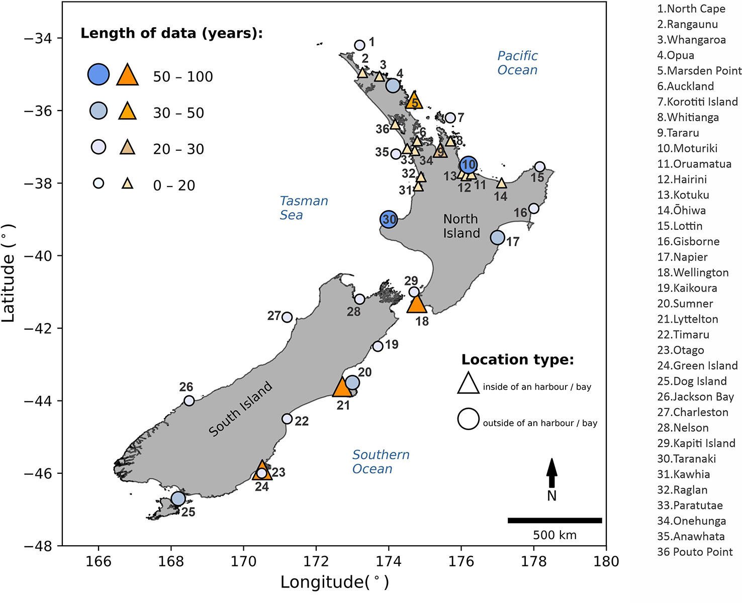
Figure 1 Location of the tide gauges used in the data analysis.

NZ does not experience large NTRs relative to other places in the world because of its deep and narrow continental shelf. NTRs are limited to mostly< 0.5 m, approximately 25% of the average tidal range (Stephens et al., 2020). However, Stephens et al., 2020 showed that larger NTRs and skew-surges can occur — the maximum NTR ever observed was 2.26 m at Jackson Bay on 1^st February 2018; the largest skew-surge was 1.15 m and occurred at Raglan on the 6^th of May 2013. The seasonality of extreme water levels and NTR in NZ closely follows the seasonal mean sea-level anomaly (MSLA) pattern. Consequently, even small sea-level rise (SLR) will potentially increase the frequency of presently rare extreme sea levels. This is a particular issue for NZ because the SLR trend is 1.88 ± 0.1 mm yr^-1 (Bell et al., 2022), and most parts of the country are subsiding due to tectonic activity (Beavan and Litchfield, 2012). The SLR, vertical land motion and extreme water levels threaten the NZ’s estuaries and harbours due to their ecological importance or because coastal communities and maritime trade are concentrated in these regions (e.g., Auckland, Tauranga, Wellington, Dunedin).

3 Methods

The methods applied in the present manuscript can be divided into two parts: a regional analysis, based on observed data, and the analysis of the TSI and morphological effects, based on data and a numerical modelling investigation. Figure 2 shows a general flow chart of the methods. Firstly, the database is described (Section 3.1) as well as the processing of the water levels observed with 36 tide gauges (Section 3.2). After, in Section 3.3–3.4, the methods that were applied in the regional assessment of the TSI (which includes NTR, skew-surge, and astronomical tide) are described. In Section 3.5, the methods for analysing the effects of the interaction between the estuarine morphology, tide, and surges (i.e., NTR and skew-surge) on the magnitude and co-occurrence of extreme water levels within an estuary are shown.

FIGURE 2

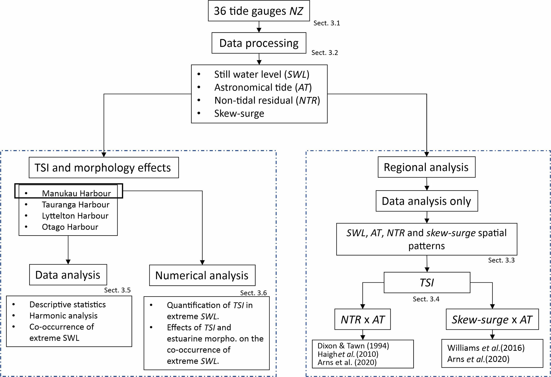
Figure 2 Flow chart of the methods.

3.1 Study site and database

The present study analysed the observed water level of 36 different tide gauges around NZ (Figure 1). The period of observations ranges from 6 to 87 years. A complete list of tide stations and associated metadata are shown in the Supplementary Table 1. The NZ sea-level records analysed here are from various locations, including wave-exposed open coasts, inside port breakwaters, or mounted on wharves inside estuaries, so they have different levels of wave exposure, which requires specific data pre-processing, which is described in Section 3.2. All observations were used for the regional analysis in the first part of the study.

Four different locations were selected for the second part of the study, which was to analyse the combined effect of the estuarine morphology (i.e., bathymetry and geometry), tide, surges and their interactions: (1) Tauranga Harbour, with Moturiki and Hairini tide gauges; (2) Manukau Harbour, with Anawhata and Onehunga tide gauges; (3) Lyttelton Harbour, with Sumner and Port Lyttelton tide gauges; (4) Otago Harbour, with Green Island and Port Dunedin tide gauges. The reason for choosing these estuaries is that they had at least one tide gauge record inside and outside the estuary with an overlap duration of ≥ 10-year.

The four estuaries have different morphology and dynamical characteristics. Manukau and Tauranga harbours have constricted mouth, extensive total areas (~365 km² and ~200 km², respectively), and vast intertidal zones in proportion to the entire surface area of the estuary (60% and 77%, respectively). However, Manukau Harbour is more extensive and has a deeper main channel (up to 30 m close to the mouth) than Tauranga Harbour (15 m at the Port of Tauranga). Tauranga Harbour also has estuarine subsystems (e.g. Hairini and Oruamatua) caused by the underlying volcanic geology of the region. Otago and Lyttelton harbours are smaller in their total area and have less than half of their estuary area covered by tidal flats (45% and 16%, respectively).

To further study the effects of the estuarine morphology on the tides, NTR, and TSI, a numerical modelling study was set up for Manukau Harbour, detailed in the Section 3.5. For the model, topo-bathymetric and hydrodynamic data were needed. For the coastal and estuarine areas of the model grid, the depth data used were obtained from digital nautical charts (n° 4314 and 4315) surveyed by New Zealand Navy and topography data from LiDAR aero surveys executed by Land Information New Zealand (LINZ). The LiDAR data were taken between 2016–2017 with a spatial resolution of 1 m × 1 m and accuracy of 20 cm (vertical) and 60 cm (horizontal). Both bathymetry and topography data for the Manukau coast and Harbour are freely and publicly available from the LINZ data portal (https://data.linz.govt.nz/). For the oceanic part of the numerical grid, bathymetry data (250 m spatial resolution) from the National Institute for Water and Atmospheric Research (NIWA) was used (https://niwa.co.nz/). The hydrodynamic data used in the model’s boundary conditions are the still water level (SWL) derived from the data pre-processing described in Section 3.2.

3.2 Data pre-processing

The data pre-processing for the water level records follows Stephens et al. (2020) and consisted of five steps applied for each of the 36 tide gauges. Firstly, a 15 min running average filter was used to reduce the effect of infragravity and tsunami waves; secondly, all the water level data were subsampled to 1 h intervals to homogenize all the time series to the same time resolution; thirdly, the effects of historical SLR were filtered out from the water level records by subtracting the 1-year-running average of the water level record. The third step results in a filtered water level record (SWL), where water level variations are relative to MSL=0 m. Fourthly, the SWL was separated into its main components (i.e. astronomical tide and NTR) by predicting the 67 standard astronomical components of the tide using the Unified Tidal Analysis package (Codiga, 2011) and subtracting the astronomical tide from the SWL to obtain the NTR. In addition, the skew-surge was estimated by calculating the height difference between the peak of the SWL and the closest high tide.

3.3 Regional distribution of extreme SWL, astronomical tide, NTR, and skew-surge

To analyse the regional distribution of SWL, astronomical tide, NTR, and skew-surge, the 98th, 99th, and 99.8th percentiles of these four variables were calculated. The percentiles were chosen to focus on extreme values of the SWL, astronomical tide, NTR, and skew-surges records at each of the 36 tide gauges. The 99.8^th percentile was chosen for the analysis because it represents the extreme SWL for NZ well, according to Stephens et al. (2020), which is further explained in Section 3.4.

3.4 Tide-surge interaction (TSI)

The techniques used to analyse the degree of tide and surge interactions can be divided into two categories. The first considers a null hypothesis that the extremes of NTR or skew-surge and their corresponding astronomical tide are independent, which means that any surge (i.e., NTR or skew-surge) could happen at any tidal level (Dixon and Tawn, 1994; Haigh et al., 2010; Williams et al., 2016). In the second category, the statistical dependence between astronomical tides and surges is analysed (i.e., NTR or skew-surges) during extreme SWLs. The null hypothesis is that tides and surges are dependent, which means that TSI occurs, and the highest surges will not necessarily coincide with the highest tides (Arns et al., 2020).

The tide-surge statistical dependence was tested in each one of the 36 tide gauges using four different techniques: Dixon and Tawn (1994); Haigh et al. (2010); Williams et al. (2016); Arns et al. (2020). The first two techniques aim to detect the degree of the TSI by analysing the differences in distributions of the extreme NTR at different tidal heights or at different times of occurrence relative to the high tide, respectively. The third method assumes independence between surges and astronomical tides and calculates the correlation between the extreme skew-surges and the corresponding astronomical tide. The fourth method assesses the dependence between astronomical tides and surges (i.e., NTR or skew-surge) in the extreme SWL.

The Dixon and Tawn (1994) method splits the tidal range into five bins between low astronomic tide and high astronomic tide. The highest 1% of hourly NTR are placed in each range based on the tide height associated with the time of their occurrence. To establish the statistical significance, a chi-squared (χ²) test is performed:

$\begin{array}{ll}{\chi }^2={\displaystyle {\sum }_{n=1}^5{(N_i-e)}^2/e}& (1)\end{array}$

Where N_i is the number of NTR heights in bin i and e is the expected number if there was no TSI:

$\begin{array}{ll}e={\displaystyle {\sum }_{i=1}^5{N}_i/5}& (2)\end{array}$

The expected number of events for the null hypothesis (no interaction) — at the 95% significance level — from the chi-squared distribution is ${\chi }_{4,0.95}^2\le$ 9.5, where the number of degrees of freedom is 4 (1 less than the number of bins). Therefore, if χ² from Equation 1 is less than 9.5, there is a 95% probability of no interaction, but a value greater than 9.5 in indicative of an interaction.

The Haigh et al. (2010) method selects the 1% highest NTRs and clusters them in hourly bins for 6 hours before and after the time of the high tide. The method assesses whether there is a significant relationship between NTR and tides, similarly to Dixon and Tawn (1994), using the chi-squared test (Equation 1). However, the null hypothesis, which is no interaction, is considered as ${\chi }_{12,0.95}^2\le$ 21 — since there 13 values, there are more degrees of freedom —. Thus, if χ² ≥21, interactions between astronomical tides and storm surges are more likely to occur.

The Williams et al. (2016) and the Arns et al. (2020) methods test whether skew-surges and tides are independent using different statistical tests. Both establish statistical dependence between these variables by calculating Kendall’s rank correlation (τ) (Kendall, 1938). The coefficient can have values between -1 and 1, where 0 indicates no correlation and 1 (-1) a perfect relationship (disagreement). There is no interaction if the correlation is insignificant (p ≥ 0.05). Conversely, when the correlation is significant (p ≤ 0.05), TSI occurs. Rank-ordered methods have been widely applied to study non-linear statistical relationships in coastal science because they are less sensitive to outliers and skewed distribution than Pearson’s correlation and do not depend on assumptions of linearity between the variables.

Williams et al. (2016) assume that astronomical tides and skew-surges are independent during extreme skew-surges. The method selects the largest 1% of the skew-surges and the corresponding astronomical tide and calculates the coefficient between the variables. Here, the skew-surge was calculated for every SWL peak by subtracting it from the closest high-tide level within ± 6 h. Then, the Kendall coefficient was calculated by selecting skew-surges over a threshold of the 98^th, 99^th, and 99.8^th percentiles and the corresponding astronomical tide.

The Arns et al. (2020) method assumes that NTR (and skew-surges) depend on the astronomical tides at the largest SWL. The method first selects the extreme SWLs in a time series. In this study, the Stephens et al. (2020) approach was used in which extreme events of SWL were selected by applying peaks over threshold (POT) using the 99.8^th percentile with a declustering scheme of 3 days between events (to ensure that events are independent from each other). This is required for a statistically robust calculation of extreme values using maxima techniques like POT (Coles, 2001). According to Stephens et al. (2020), these are the threshold and periods that are ideal for selecting SWL extreme events in NZ, and which results in an average of 5 events per year for NZ’s tide gauges. Extreme events were also selected by using the 98^th and 99^th percentiles of the SWL to check how the TSI affects different percentiles of SWL and vice versa.

Furthermore, the Arns et al. (2020) method can statistically quantify the TSI effect in the extreme SWL. The statistical model was built based on global analyses of tidal gauges. It uses a copula-based method to generate extreme synthetic SWL considering a scenario where the astronomical tides and NTR are dependent (i.e., τ≠0) and another where these two variables are independent (i.e., τ = 0). The difference in the simulated SWL between the scenarios is fitted to a multiple regression model as a function of the rank correlation between the observed NTR and astronomical tide (τ) in a specific quantile. Thus, the average difference in centimetres for a given percentile of the SWL can be expressed by the following:

$\begin{array}{ll} TSI\sim a+b\ast \tau +c\ast {\tau }^2+d\ast {\tau }^3& (3)\end{array}$

With the coefficients a =-21, b = -151, c = -419, and d= -463 for the percentile 98^th; and a =-21, b = -164, c = -461, d= -517, for the percentile 99^th. To calculate the TSI for the percentile 99.8^th, which was not calculated in Arns et al. (2020), the coefficients were assumed to be the same as for the 99th percentile. Each tide gauge was treated independently, considering the whole time range.

Past work has suggested that TSI is larger in shallow areas. In this section the focus is on the enclosed shallow areas of the database, to test whether they are more likely to have TSI, what is the likely effect of that, and why might that occur (friction, morphology…).

3.4.1 Estuarine morphologic attributes and TSI

The correlation between the TSI found by applying the Arns et al. (2020) statistical model and the morphologic attributes of estuaries was analysed. For this analysis, only tide gauges located within estuaries were considered, which resulted in 14 tide gauges. We choose four morphologic attributes: the coverage of the intertidal zone area (which is related to the surface area of the estuary); the average depth of the estuary; the surface area of the estuary; and, the mouth width of the estuary. The attributes were obtained from the Hume et al. (2016) database.

3.4.2 Transformations in tides, NTR, and skew-surges in shallow enclosed areas

The goal of this Section was to determine whether the TSI is generated within or just outside these estuaries. For this analysis only the harbours with one tide gauge record inside and outside the estuary with observation periods that overlap for at least ten years were selected, as described in Section 3.1. This selection resulted in four different estuaries: Manukau, Tauranga, Lyttelton, and Otago Harbour. This analysis was aimed at observing the attenuation/enhancement of the extreme events that occur in areas outside and propagate within the estuary, and the role that morphology of the estuary and other local physical processes may play in that process. The effects of the estuary’s morphology in the SWL were identified by performing two different analyses.

Firstly, the probability distribution and the quantiles of the SWL, astronomical tide, NTR, and skew-surge of the tide gauges inside and outside the harbour were compared. The probability distribution comparison was used to identify tidal asymmetry (measured by the skewness of the distribution) and the quantile comparison to identify amplification/dampening of the SWL, astronomical tide, and increase/decrease of the NTR within the harbour. To quantify the quantile comparison, the differences between the 99.8th quantile of the gauges located both inside and outside were calculated.

Secondly, the rate of co-occurrence between extreme SWLs outside and inside the harbours was determined. This analysis shows the practical implications of TSI within estuaries. For each of the four estuaries, the extreme SWL events were extracted in two ways. First, similar to Section 3.4 — by applying POT (99.8^th percentile) and a declustering scheme of three days — but only considering the period when the records from the tide gauges located inside and outside the harbour coincide. Second, the co-occurrence of the SWL annual maximum between the tidal gauges was considered. For the POT selection, time windows of 6 h before and after each extreme event were applied to ensure that the distances between tide gauges and storm durations were considered. For the maxima selection, the number of SWL annual maxima that co-occur within 12 h prior or later to each maxima event were counted.

3.4.3 Harmonic analysis

One indicator that TSI is likely to be important is if nonlinear transfer of tidal energy between different tidal harmonics occurs. This is because TSI is caused by the same terms in the shallow water equations as tidal distortions. For instance, the non-linear interactions between the principal astronomical constituents (e.g., M2, S2, and N2), bed friction, and morphology can generate shallow-water constituents (e.g., M4, MS4, MN4). The approach of Speer and Aubrey (1985) was applied to calculate the degree of interaction between M2 and M4 amplitudes (aM4/aM2) and phases (2gM2/gM4) for all 36 tide gauges in this study. The Kendall ranked coefficient was then calculated between the aM4/aM2 and the τ coefficient calculated following Arns et al. (2020), where τ is calculated using the skew-surge and astronomical tide associated with the extreme SWLs (Section 3.4). The aim of this analysis is to test whether TSI and aM4/aM2 are correlated. In addition, the differences of aM4/aM2 and 2gM2/gM4 were analysed between tide gauges located inside and outside our four focus estuaries: Tauranga, Manukau, Lyttelton, and Otago Harbour. The simple amplification of the M4 component inside an estuary can indicate that the non-linear interactions are an important process. The phase relation between the M2 and the M4 indicates the flood and/or the ebb dominance. The relation between amplitudes of M2 and M4 can indicate if there is spectral energy transfer in the tidal wave between these two harmonics.

3.5 Hydrodynamic modelling

To further investigate the interactions between tide, surges and morphology within estuaries, a hydrodynamic model was constructed for Manukau Harbour to address two objectives. First, to quantify the TSI occurring at the coast and inside the harbour. Second, to elucidate the physical mechanism of how the estuarine morphology affects the TSI and potentially contributes to the co-occurrence of extreme SWLs inside and outside the harbour. This estuary was chosen because tidal amplification is known to occur there and it has already been studied (Bell et al., 1998). In addition, Manukau Harbour is located in Auckland, the most populated city in NZ, with the biggest international airport. These factors give Manukau Harbour remarkable social-economic importance. The software DELFT3D-FLOW was used for the hydrodynamic model and 8 scenarios (SC1–SC8 detailed in Table 1). The model solves the hydrodynamic equations in two dimensions by averaging the depth velocity. Since Manukau Harbour does not receive large fluvial discharges and summer stratification is unlikely to happen because of the strong tidal currents and shallow domain (Bell et al., 1998), using a two-dimension model can be considered appropriate for this case (a test with a 5-layer 3D domain made < 1 cm difference in water levels within the domain).

TABLE 1

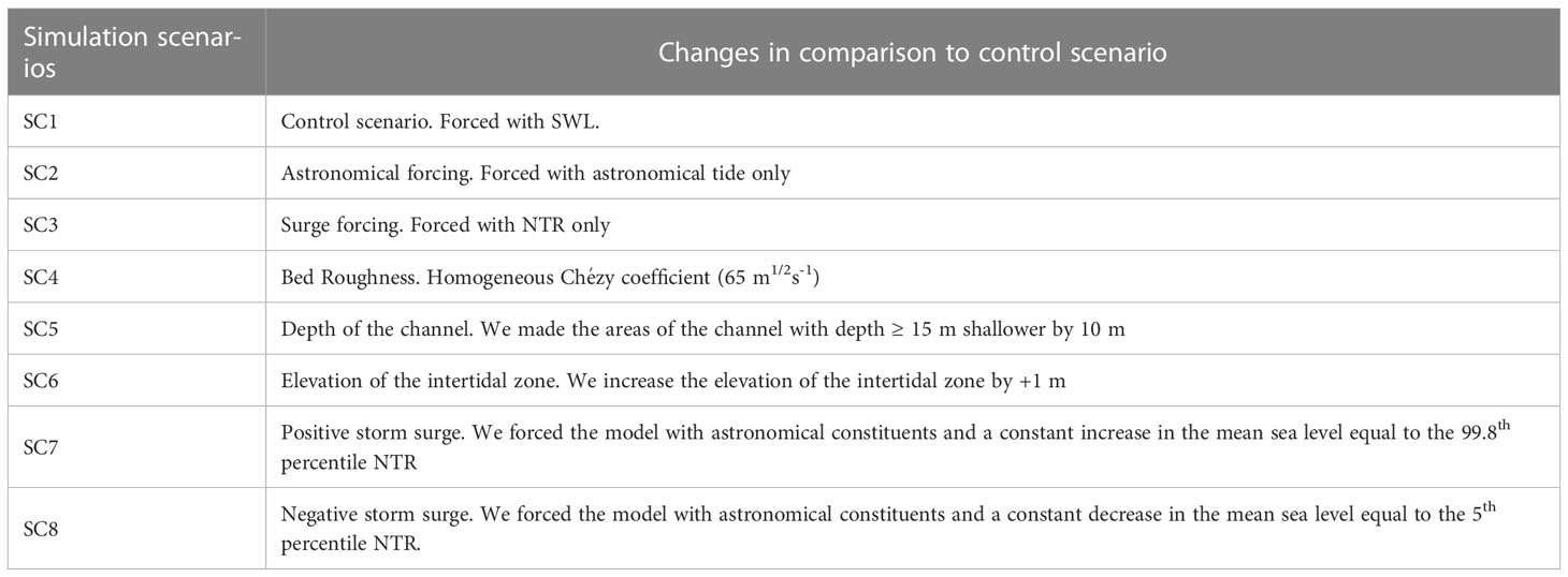
Table 1 Simulation scenarios for modelling the effects of TSI and estuarine morphology on the co-occurrence of extreme SWLs.

For the boundary conditions, topo-bathymetric and hydrodynamic data were acquired as described in Section 3.1. Figure 3 shows the topo-bathymetric data interpolated in the model domain and the location of Paratutae (33), Onehunga (34) and Anawhata (35). In addition, Cornwallis, Weymouth and Clarks Beach locations are also shown in the Figure 3 to help describe results according to the region of Manukau Harbour. The model was forced at the northern boundary with the astronomical tidal constituents, SWL, and NTR (depending on the scenario) calculated for the Anawhata tide gauge, as described in Section 3.2. The northern boundary was chosen because the tide on the west coast propagates from north to south. Open boundaries were set using Neuman conditions at the western and the southern boundaries at the coast. The direct effects of local wind were not considered (e.g., wind-setup, currents, and vertical flows), because the focus is to isolate the effect of morphology on TSI and, moreover, there are insufficient observations to warrant an increase in model complexity (e.g., no in-situ current measurements exist).

FIGURE 3

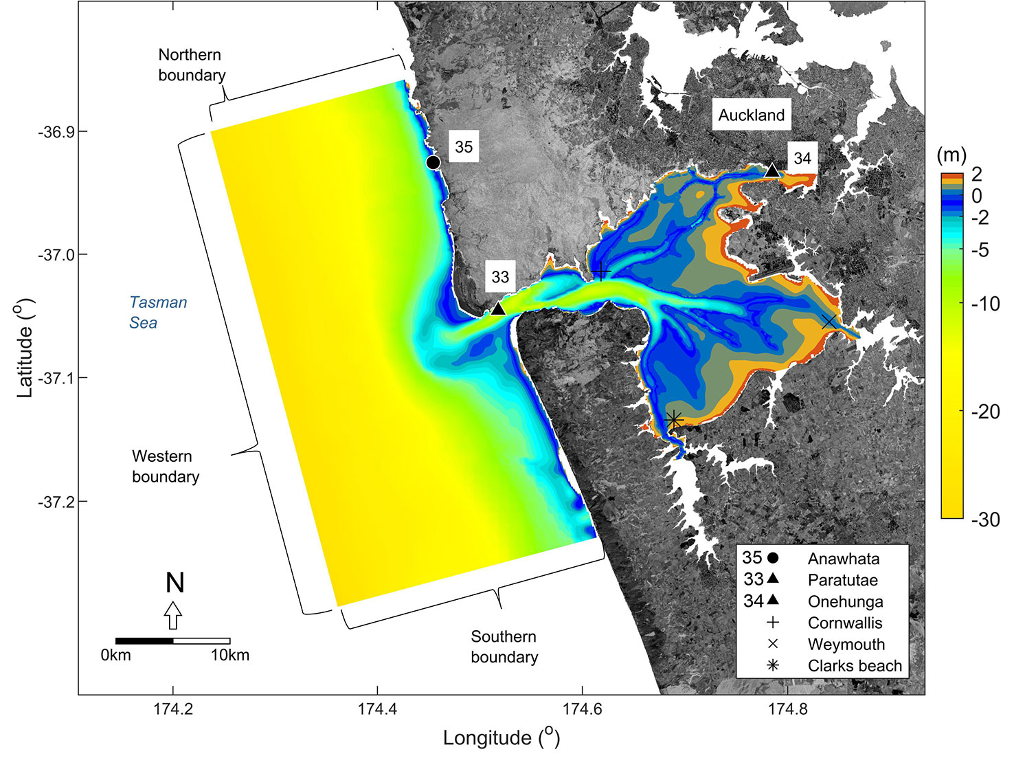
Figure 3 Hydrodynamical model setup. Interpolated topo-bathymetric data in the model domain. Positive (negative) values are used for areas above (below) the mean-sea level. The location of Paratutae (33), Onehunga (34), and Anawhata (35) tide gauges is also shown. Note that the numbering is used based on Figure 1. Cornwallis, Weymouth and Clarks Beach are reference sites used to help describe the results. Background image: aerial photos from Land Information New Zealand (LINZ). Projection: WGS84.

Although the model was used in an exploratory sense to understand the relevant physical drivers, it was still calibrated against available data to ensure simulations were realistic. Model calibration was performed by testing a range of bed roughness values by modifying the Chézy coefficient = 40–80 m^1/2s^-1 (see Supplementary Figure 1). The optimum Chézy was selected by comparing the modelled and observed differences in amplification between Anawhata and Onehunga tidal gauges at the maximum SWL, and by calculating the root mean squared error over the entire simulation period. The result was a homogeneous bed roughness of Chézy coefficient = 50 m^1/2s^-1 through the model domain, which showed the best match to the observed data. Note that although the Chézy coefficient = 45 m^1/2s^-1 showed the best amplification, it was less accurate in terms of root mean squared error. See Supplementary Figures 1, 2; Table 2 for the detailed model setup and calibration.

TABLE 2

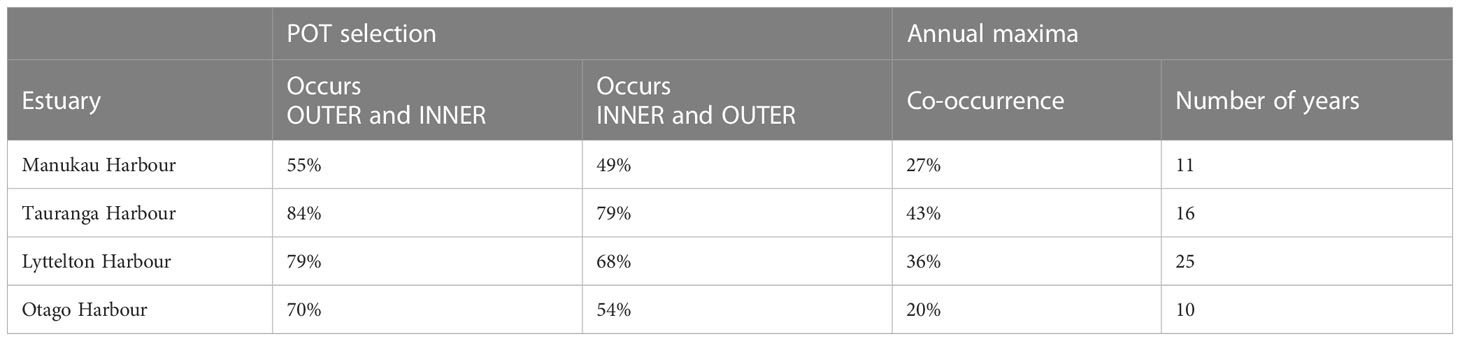
Table 2 Co-occurrence rates between extremes of SWL (99.8th percentile) and annual maxima occurring inside (INNER) and outside (OUTER).

3.5.1 Numerical quantification of TSI on extreme SWLs

To determine the magnitude of the TSI, the method of Idier et al. (2012) was used, in which three different simulation scenarios were set up. In the first scenario (SC1), the model was forced by the SWL observed at the Anawhata tide gauge. The SC1 was the control scenario, aimed at simulating a condition where tide and surge are dependent, and TSI occurs. The second scenario (SC2) was forced with the astronomical tidal constituents only. In the third scenario (SC3), the model was forced using the NTR only. The SC2 and SC3 outputs are summed to represent the SWL case in which tide and surge interactions do not occur. Finally, to estimate the magnitude of TSI, the difference between SC1 and (SC2+SC3) was calculated at the locations of the Anawhata, Paratutae and Onehunga tide gauges.

3.5.2 Modelling the effects of estuarine morphology and bed friction on the TSI

As described in Section 1, the shallow-water effect and bottom friction are likely some of the main contributors to TSI. To assess the importance of each of these elements, and how they impact the TSI throughout the Harbour domain, the scenarios SC4, SC5, and SC6 were set up. SC4 explores the effects of bed friction, by homogenously increasing the Chézy coefficient to 65 m^1/2s^-1 over the entire model domain. SC5 and SC6 explores how changes in morphology can affect TSI, by making the main channel shallower (+10 m, close to the entrance) and the intertidal zones shallower (+1 m), respectively as described in Table 1. For each one of the scenarios, the TSI was calculated for the model domain, considering the maximum TSI at each grid cell over the entire simulation period. Additionally, TSI on the peaks of SWL over the 99.8^th percentile was calculated for Onehunga.

3.5.3 Modelling the effects of TSI on the tidal amplification

To further investigate the effect of the surges on tidal amplification, the astronomical tide at a constant positive surge of NTR=99.8^th percentile (SC7) and a constant negative surge of NTR = 5^th percentile (SC8) were simulated. To compare the results of these scenarios, the maximum water level at each grid cell of each simulation scenario was calculated (i.e., control scenario and SC7 and SC8) through the entire simulation period. Then, the amplification factor of each simulation scenario was calculated independently, using equation 4:

$\begin{array}{ll}Amp.\mathrm{Fac}.=\frac{peaktideinside}{peaktideoutside}-\mathit{1}& (4)\end{array}$

where the peak tide inside is anywhere inside the estuary (location of a tide gauge or model grid cell) and peak tide outside is the model boundary condition or observed data at Anawhata tide gauge. Finally, for each simulation scenario (i.e., SC7 and SC8), the amplification factor of a given scenario was subtracted from the control scenario (SC1), to infer if the amplification increased (positive difference) or decreased (negative difference). Additionally, the non-linear terms (i.e., shallow-water effects, and bed friction) are assessed for their impact the NTR by calculating the amplification factor (Equation 4) for the SC3, which simulates only NTR over the model domain.

4 Results

4.1 Regional patterns of SWL, NTR, skew-surge, astronomical tide, and TSI occurrence

Figure 4 shows the regional patterns of SWL, astronomical tide, NTR and skew-surge for the 99.8^th percentile of each variable. The patterns of extremes in SWL follow the extremes of astronomical tide (Figures 4A, B). The largest values of SWL and AT were found on the west coast, because the tidal range is larger. On the east coast, where the tidal range is smaller, the percentiles of SWL and AT are the smallest. Regarding the NTR, the highest values occur in the tide gauges located inside estuaries, for instance, in Raglan and Kawhia (Figure 4C). The values of the skew-surge are similar to the NTR. Of the 36 tide gauges, differences between skew-surges and NTR of ≅ 0 cm occurred at 18 of them. A small difference between 1 cm and 4 cm occurred at the remaining 18 sites. The maximum difference occurs at the location of the Onehunga and Hairini tide gauges. The Supplementary Table 3 the 99.8^th percentile for each variable and the difference between NTR and skew-surge for each tide gauge.

FIGURE 4

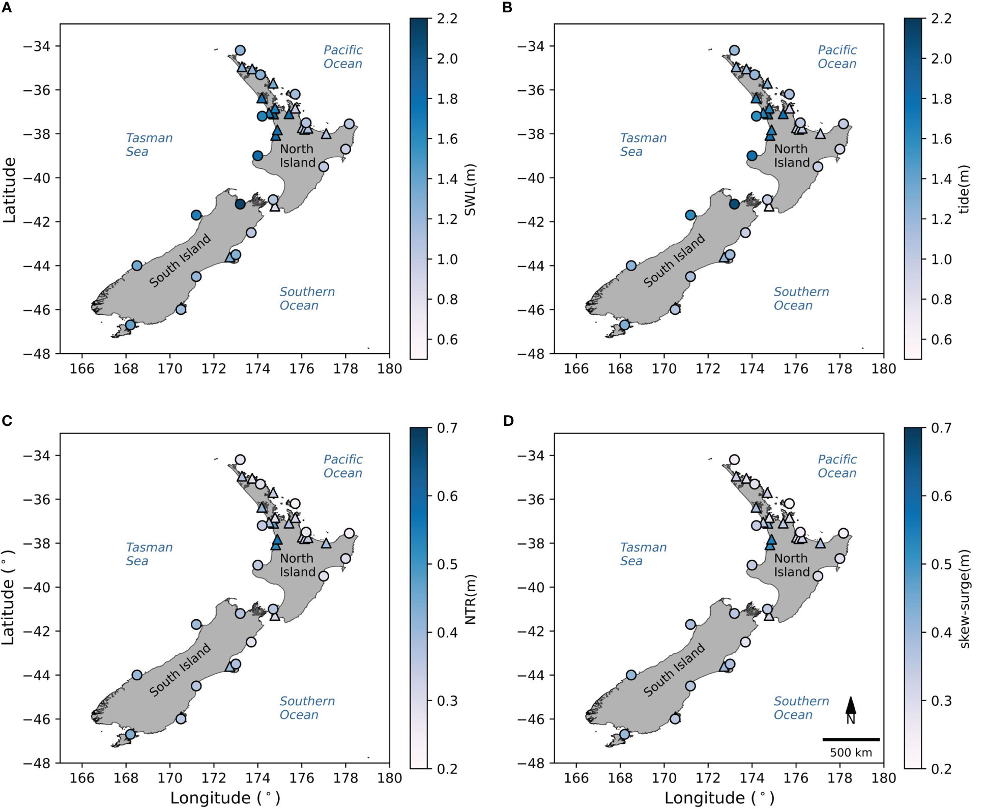
Figure 4 Quantile of 99.8% for SWL (A), astronomical tide (B), NTR (C), and skew-surge (D) for tide gauges around NZ. Triangles (circles) mark tide gauges located within estuaries (outside estuaries).

The highest 1% of the NTR and the corresponding astronomical tide were dependent in most of the tide gauge records located in estuaries, ports and bays, assessed using both the Dixon and Tawn (1994) (χ²≥ 9.5), and Haigh et al. (2010) (χ^2 ≥ 21) approaches (Figures 5A, B, respectively), which means that TSI generally occurs at these sites. However, Dixon and Tawn (1994) showed that TSI does not occur at most of the exposed coastal locations (of these, TSI was only observed at Anawhata, Charleston, Dog Island, and Timaru). Conversely, the Haigh et al. (2010) approach showed dependence (χ² ≥ 21) at most of the tide gauges, even at the exposed coastal locations (NTRs are independent (i.e., TSI does not occur) at only North Cape, Sumner, Whangaroa, and Lottin (Figure 5B), and only for the largest 1%). All values of χ² found for both methods (Haigh et al. and Dixon and Tawn) are provided in Supplementary Table 4.

FIGURE 5

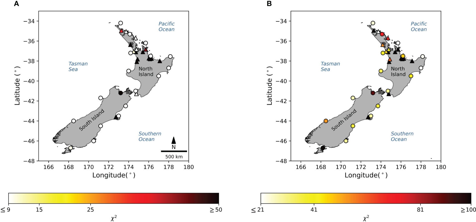
Figure 5 Tide and surge χ2 in different tide gauges according to Dixon and Tawn (1994) (A) and Haigh et al. (2010) (B). In (A) values ≤ (≥) 9 indicate that NTR and tide are independents (dependents). Similarly, in (B) values ≤ (≥)21 indicate that NTR and tide are independents(dependents). Triangles (circles) mark tide gauges located within estuaries (outside estuaries).

At inner estuarine locations, the largest NTRs usually occur 4 – 6 h after (+) the peak of the tide, close to the low tide. For instance, Figure 6 compares the Haigh et al. (2010) (I) and the Dixon and Tawn (1994) (II) analysis for Anawhata (A), Onehunga (B), Otago (C), Green Island (D), and (E) Gisborne. The Onehunga tide gauge is generally representative of inner estuarine locations (B I and II). The only location that shows similar evidence of TSI, although occurring 2–3 h before (-) the peak of the tide, is in Otago Harbour (C.I). For locations outside estuaries, the effects of TSI are smaller (i.e., lower value of χ²), which is illustrated for Anawhata, Green Island, and Gisborne in Figures 6 A, D, E, respectively.

FIGURE 6

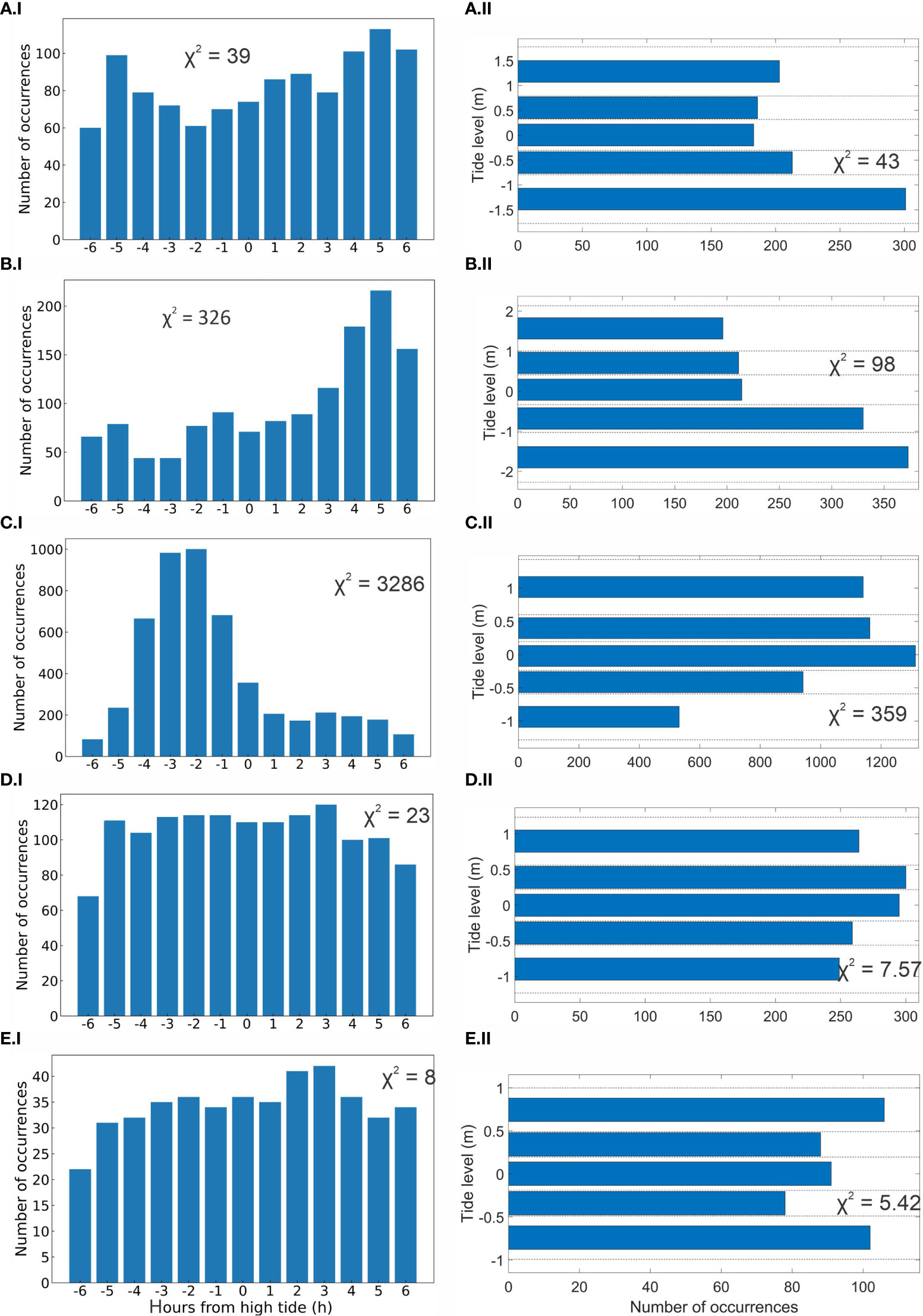
Figure 6 Bar plots show the resulting analysis from Haigh et al. (I) and Dixon and Tawn (II) approaches. The Haigh et al. approach shows the time difference between the largest 1% NTRs and the high tide. Dixon and Tawn’s approach shows the tidal interval where the highest 1% of the NTR occurs. The panels show the resulting analysis for (A) Anawhata, (B) Onehunga, (C) Otago, (D) Green Island, (E) Gisborne. The χ² of each analysis is also shown.

The Arns et al. (2020) approach shows a significant correlation between the NTRs and tides at all tide gauge locations during extreme SWLs (98^th, 99^th, and 99.8^th percentiles; Figure 7A I–III, respectively). The Kendall coefficient (τ) varies between -0.35 and -0.60 over all the tide gauges, meaning that the higher is the tide, the lower will be the NTR and vice-versa. The relationship is stronger (more negative) for the percentile 99.8^th (III) and becomes weaker for the percentiles 99^th (II), and 98^th (I), in this order. Tide gauges in the inner estuarine locations (e.g., Raglan, Kawhia, Rangaunu, Whangaroa, Ohiwa) and ports (Gisborne, Napier) have the strongest τ. This analysis was performed for the relationship between skew-surge and astronomical tides, showing similar dependence of the extreme SWLs (see Supplementary Table 5).

FIGURE 7

Figure 7 Kendall ranked coefficient (τ) (A) and TSI (B) calculated following Arns et al. (2020) (NTR x astronomical tide) corresponding to the storm events that produced an SWL ≥ 98th (I), 99th (II), and 99.8th (III) percentile. Triangles (circles) mark tide gauges located within estuaries (outside estuaries).

The Arns et al. (2020) statistical model showed that the TSI is positive at most of the tide gauge locations for the different percentiles of SWL. Again, the largest TSI was found for tide gauges located inside estuaries. For instance, Figure 7B. I–III shows that most of the TSI ranges between 0 to 10 cm and show small variations through all gauges locations for the 98^th (I) and 99^th (II) percentiles, reaching up to 12 cm at Ōhiwa. In the 99.8^th percentile of SWL (B.III), the values of TSI increase at most of the tide gauges, reaching up to 27 cm at Hairini. The number of locations showing no interaction between tides and NTR (i.e., TSI values ~0 cm) is greater for the 98^th and 99^th percentiles than for the 99.8^th percentile. At the sites where TSI ≅ 0, the associated τ is ≥ -0.35. See Supplementary Table 5 for the values of TSI at each tide gauge location.

The last method trialed, the Williams et al. (2016), was specifically designed to analyse the dependence between the skew-surges and tides. Note that skew-surge accounts for TSI by calculating the difference between peak of the SWL and the peak of the high tide, which should not be affected by phase difference caused by distortions in tide and NTR within the harbour. Ultimately, evaluating tide and skew-surge dependence is fundamental for the validation of SSJPM for use in prediction (see Section 1). According to the method, the highest skew-surges and the corresponding astronomical tides are independent at most locations of NZ. Significant correlations were only found between the highest skew-surges (over the 99.8^th percentile) and astronomical tides at the Hairini tide gauge location. However, the correlation is low, with τ= -0.16 (see Supplementary Table 6). Surprisingly, the number of sites showing significant correlation increased as the threshold applied in the POT selection (99^th and 98^th percentiles) decreased. For instance, for the extreme skew-surges selected over the threshold of the 98^th percentile, a total of six sites showed a significant correlation (p ≤ 0.05). Although most sites show negative and low coefficients (range between -0.05 to -0.16).

4.2 Astronomical tide, NTR and skew-surge in shallow and enclosed areas

The only estuarine morphologic attribute (see Section 3.5.3) that showed any significant correlation (p ≤ 0.05) with the coefficient τ calculated using the Arns et al. approach — dependence between NTR and astronomical tide at the 99.8^th percentile of SWL — across all 26 sites was the intertidal zone area, which showed a correlation of τ = -0.46. This means that the larger the intertidal zone area is in relation to the estuarine total area, the strongest is the TSI (more negative).

In addition, the detailed analysis of Lyttelton, Otago, Manukau, and Tauranga harbours shows that estuarine bathymetry and geometry affect the SWL. The effects on SWL differ according to the harbour, mainly driven by deformations that affect the tidal wave as it propagates within the estuary. They include tidal amplification, dampening, and asymmetry. The effects are observed to be stronger in Manukau and Tauranga Harbour, which are places with the largest intertidal areas.

Tidal amplification occurs in Manukau, Lyttelton, and Otago Harbours. The probability distribution and quantile-quantile plots of SWL, astronomical tide, and NTR for these locations are shown in Figures 8, 9. For instance, the largest amplification occurs in Manukau Harbour. Figure 8 (C.I, C.IV) shows that the distribution of the SWL and astronomical tide (resp.) are wider at Onehunga (ranging from < -2 m to > +2 m) than at Anawhata (ranging from > -2 m to < +2 m). The amplification can be equal to 32 cm for the upper tail of the distribution (95^th –99.8^th percentiles) and 18 cm on average considering all quantiles, Figure 9 (C.I, C.IV). For Otago and Lyttelton Harbours, the amplification is lower, reaching a maximum of 13 and 4 cm in the upper tail, respectively, Figure 9 (A.IV, B.IV).

FIGURE 8

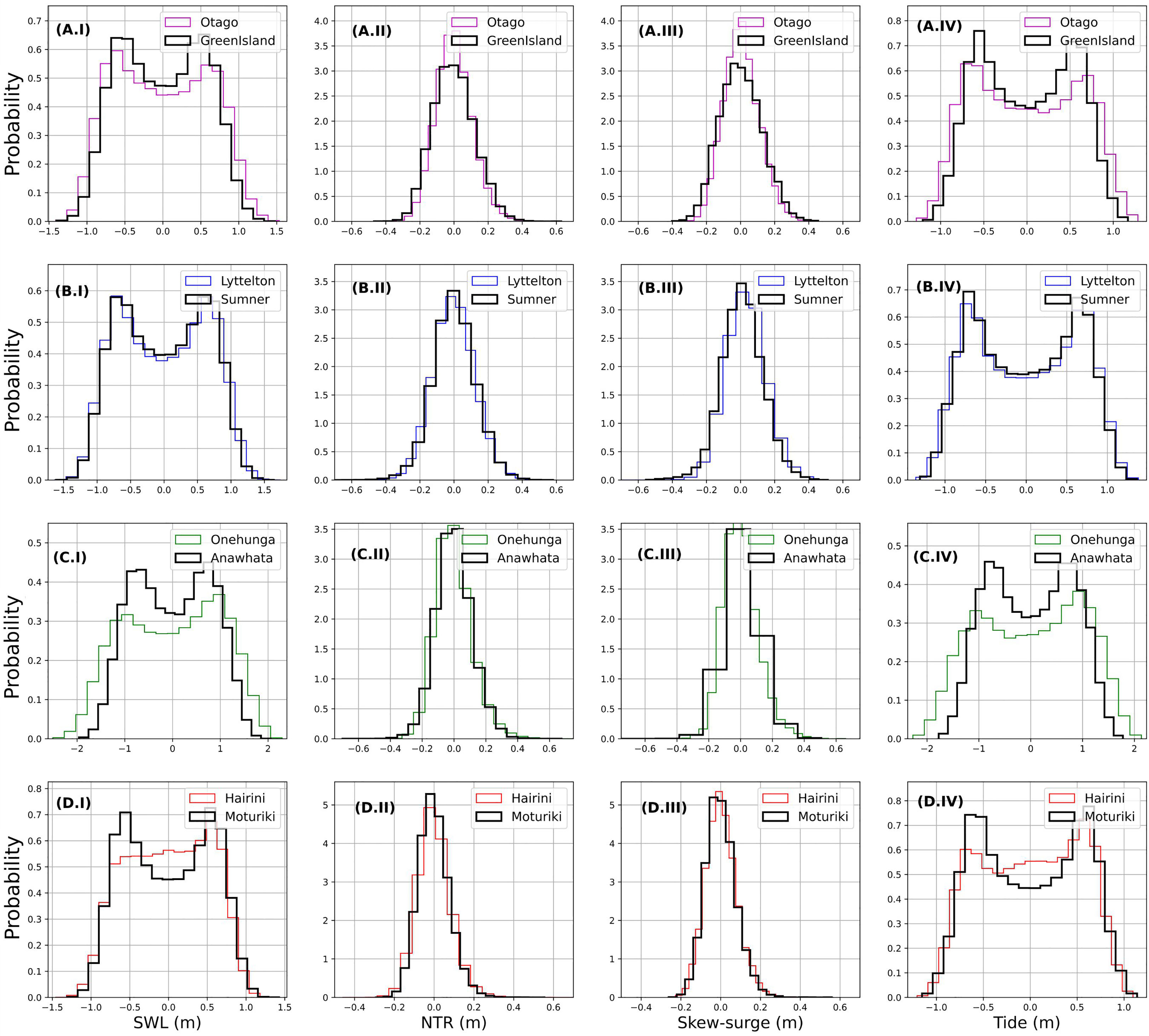
Figure 8 Probability distribution of SWL (I), astronomical tide (II), NTR (III) and skew-surge (IV) at Otago (A), Lyttelton (B), Manukau (C), and Tauranga (D) Harbour.

FIGURE 9

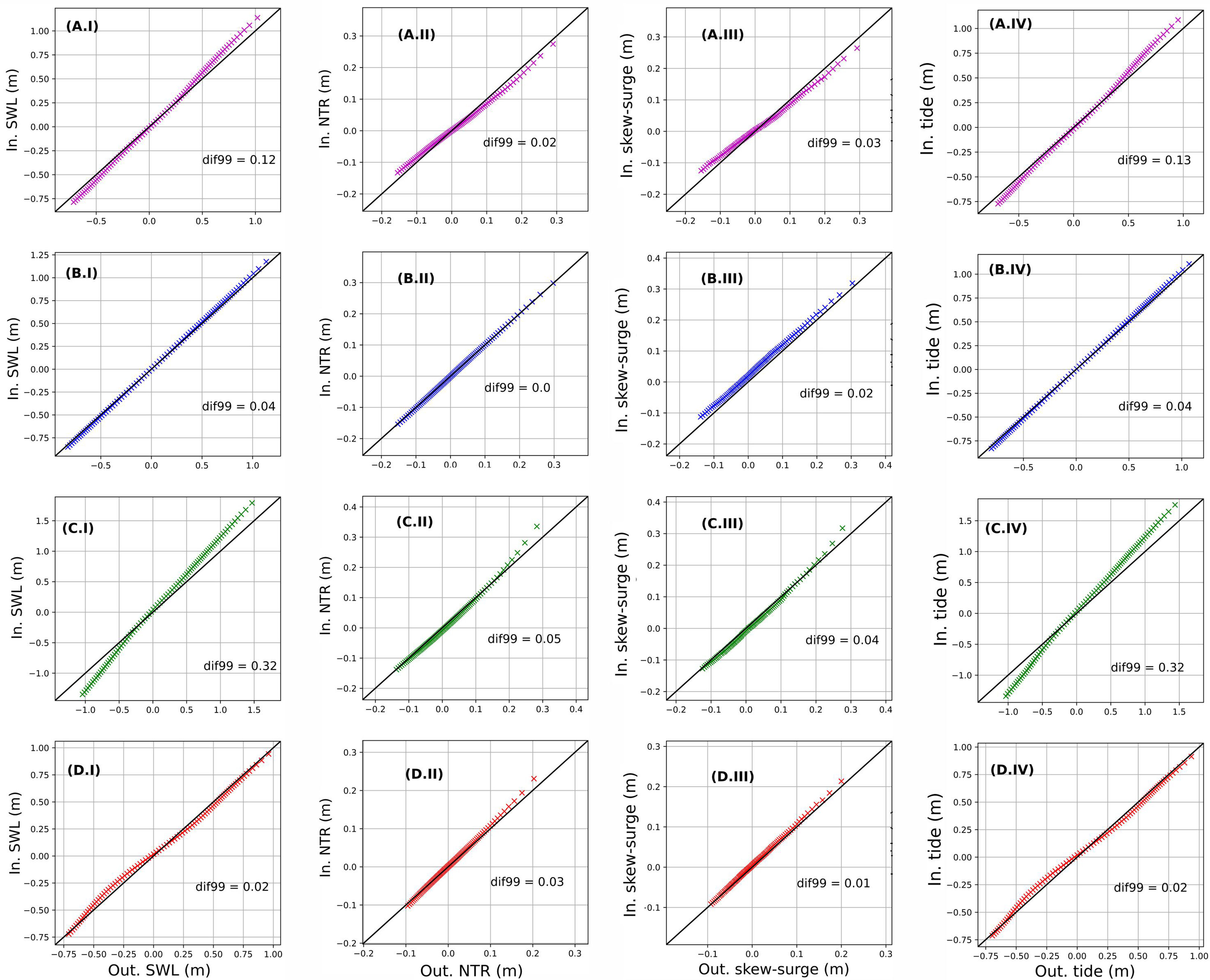
Figure 9 The quantile-quantile plot of SWL (I), astronomical tide (II), NTR (III) and skew-surge (IV) at Otago (A), Lyttelton (B), Manukau (C), and Tauranga (D) Harbour. For each panel, the absolute difference at the 99^th percentile (dif99) between the measure variable inside and outside the harbour is shown.

Tidal dampening is observed in Tauranga Harbour. Figure 8 shows a slight shortening of the distribution of SWL (D.I) and astronomical tide (D.IV), which ranges from around -1 m to +1 m. Indeed, the quantile-quantile plot (Figure 9) shows that the dampening is about 3 cm on average and a maximum of 6 cm considering all quantiles, Figure 9 (D.IV). For the upper tail (99^th percentile), the dampening is about 2 cm.

Tidal asymmetry occurred in Manukau, Otago and Tauranga Harbours, shown in Figure 8 (A, C, and D rows). For instance, the positive and negative part of the bimodal tidal distribution at Anawhata, Figure 8 (C.IV), shows equally distributed values with a statistical mode of approximately -0.8 m and +0.8 m (resp.) and a probability of ~0.45. However, the distribution is positively skewed inside the estuary (i.e., Onehunga). Thus, positive values are more likely to happen than negative ones. For instance, the probability of the positive and negative modes is 0.38 and 0.33, respectively, Figure 8 (C.III). Similar positive skewness occurs in Tauranga Harbour, but with a larger difference between positive and negative mode probabilities, 0.7 and 0.6, respectively, Figure 8 (D.IV). Figure 8 (A.IV) shows a slight negative skewness in Otago Harbour.

NTR and skew-surge are modified when the waves propagate inside the estuary. This can be observed for all estuaries in Figure 9 (column II and III), but especially for Manukau Harbour (C.II and C.III), where an increment of 5 cm and 3 cm were observed at the 99^th percentile for NTR and skew-surge, respectively.

Because of the effects of morphology on the tide (i.e. dampening, amplification, and asymmetry) and their influence on TSI, the extreme SWLs events inside and outside the estuary are not expected to always co-occur. Table 2 shows that for all four estuaries analysed, only a fraction of the extreme events related to the 99.8^th percentile co-occur within a ± 6-hour time window, either inside and outside the estuaries or vice-versa. The lowest co-occurrence rate occurs in Manukau Harbour, which varies between 49–55%. The co-occurrence rates are the highest in Tauranga Harbour, with 84%–79%, followed by Lyttelton and Otago harbour, in this order. The co-occurrence rates of SWL annual maxima are even lower. The highest co-occurrence rates occur in Tauranga (43%) and Lyttelton (36%) Harbours. The lowest co-occurrence rates occur in Otago (20%) and Manukau (27%) Harbours.

4.3 Harmonic analysis

Transformations in the astronomical tide (i.e., shoaling, dampening, and asymmetry) are the main contributors to the changes in the SWL observed in Section 4.2. Supplementary Table 7 compares the amplitude and amplification factor of the principal astronomical (M2, S2, and N2) and shallow water (M4, MS4, and MN4) constituents inside and outside the four studied harbours (i.e., Otago, Lyttelton, Manukau, and Tauranga Harbour). The three principal tidal components amplify for all these estuaries, but the M2 was affected the most. For instance, in Tauranga Harbour, M2 is damped by 2cm. In Otago, Lyttelton and Manukau Harbour, the M2 is increased by 3 cm, 9 cm, and 28 cm, respectively.

The shallow-water harmonic constituents (e.g., M4, MS4, MN4) have amplitudes ranging from<0.01 m up to 0.05 m through all tide gauges located inside or outside the estuaries. If compared to the principal constituents as M2, S2, and N2, where the amplitudes range from 0.06 m (N2 at Sumner) to 1.33 m (M2, at Onehunga), the shallow-water constituents are a minor contribution to the astronomical tide. However, the shallow constituents are amplified more than the principal constituents within the harbours. Supplementary Table 7 shows that the amplification factor in Manukau and Tauranga Harbour for M4 can increase by 1.22 and 1.64 times, respectively. Indeed, Supplementary Table 8 shows that the ratio M4/M2 increases when tide propagates inside Manukau and Tauranga harbours, which means that the constriction and bed friction effects are important in these sites for the tidal amplification. In Lyttelton and Otago harbours, a decrease of the M4/M2 is observed, which means that the effects of constriction and bed friction are not the main drivers for the tidal amplification, but the gradual changes in the bathymetry. The greatest ratio difference occurred in Manukau Harbour, where M4/M2 equals 0.027 in Anawhata and becomes 0.039 in Onehunga. Regarding the tide dominance, the difference of phase in 2gM2-gM4 indicates that Manukau, Lyttelton and Tauranga Harbours are ebb dominant, while Otago is flood dominant. The M4/M2 was significantly correlated with the TSI (τ= 0.36), considering all the 36 tide gauges in this study (see Section 3.5.3).

4.4 Hydrodynamic modelling results

4.4.1 TSI on extreme SWLs and the effect of the water depth and bed friction

The results show that TSI occurs inside Manukau Harbour is spatially heterogeneous. TSI decreases the SWL when tide and NTR are modelled together (SC1) in comparison to the scenario where tide and surge are independent and so cannot interact (SC2+SC3). For instance, Figure 10A shows that TSI is the strongest in the inner estuarine region, reaching approximately -0.35 m, when considering the maximum TSI per grid cell for the entire period of simulation. When the peaks over the 98^th, 99^th, and 99.8^th percentiles of SWL are analysed (Table 3), a decrease is observed in the SWL of up to 16 cm at Onehunga and 9 cm at the harbour entrance (i.e., Paratutae). However, TSI was not important at the Anawhata tide gauge outside the Harbour. The TSI also varied according to the tidal cycle. For instance, Supplementary Figure 3 shows that the largest interactions occur during spring tide, particularly when the tide transitions between spring to neap tides and vice-versa.

FIGURE 10

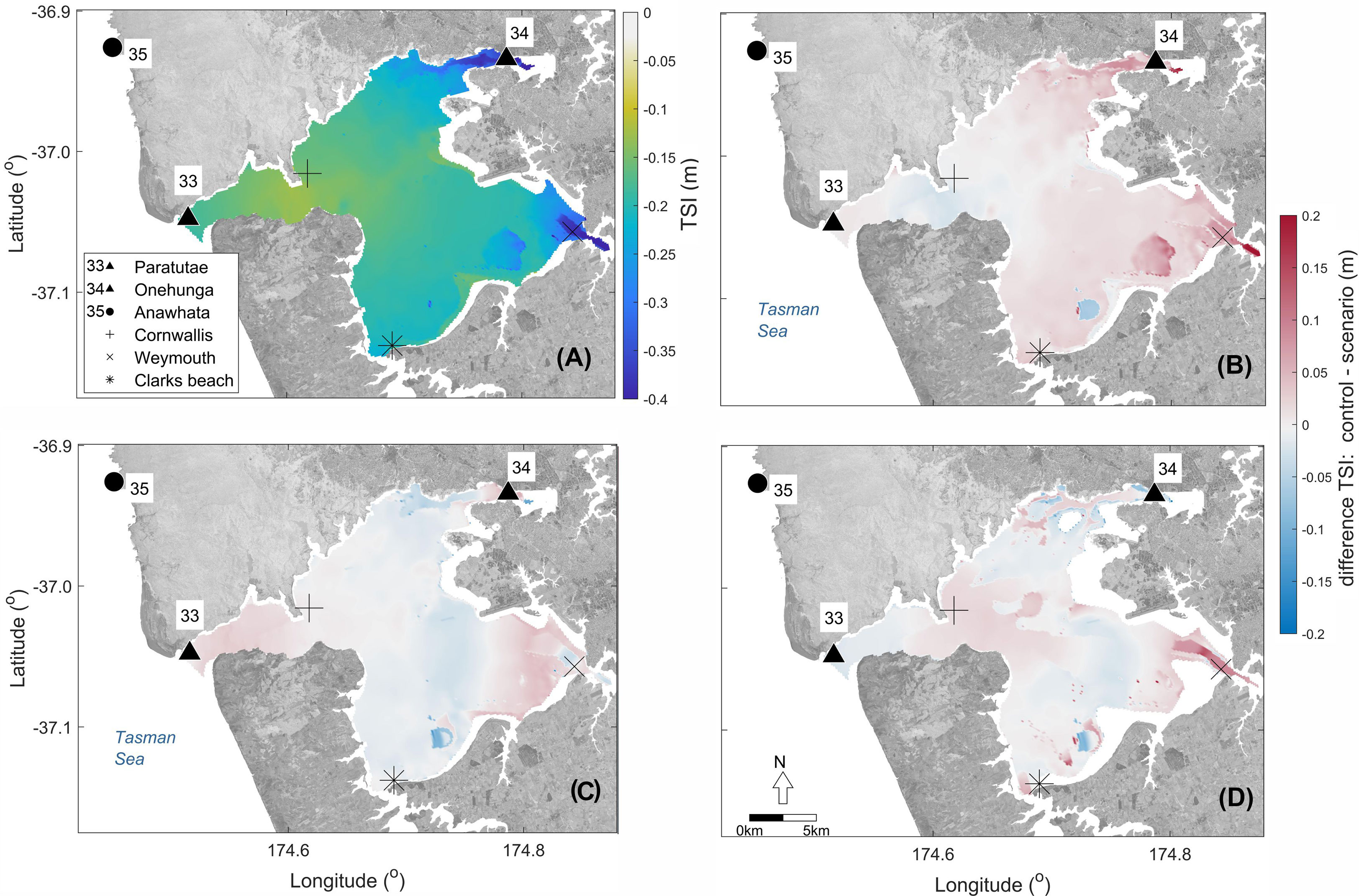
Figure 10 TSI in Manukau Harbour. TSI on the control scenario SC1 (A). Change in TSI in the model domain for SC4, when the Chézy coefficient for bed roughness is equal to 65 (B). Change in TSI for SC5, when the model was forced with the channel at the entrance of the harbour shallower (C). Change in TSI for SC7, when the model was forced with the tidal flats shallower (D). Note the ocean domain to the west has been removed to focus on the estuary. Background image: aerial photos from Land Information New Zealand (LINZ). Projection: WGS84.

TABLE 3

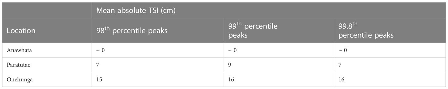
Table 3 Mean absolute TSI from numerical model.

In addition, the outputs of scenarios SC4, SC5, and SC6 (Figures 10 B, C, D, respectively) show that the effects of bed friction and water depth are equally important to the TSI and are spatially heterogeneous through the Harbour. The scenarios agree that TSI gets stronger (+) in the inner estuarine regions when bed friction, channel and intertidal zone depths are changed. Most of the differences in TSI between scenarios vary between ±0.05 m with some regions of the estuary showing larger values (up to ~0.2 m).

4.4.2 The effects of TSI on the tidal amplification

The hydrodynamic modelling results show that TSI affects the amplification of SWL in Manukau Harbour. Figure 11 shows the amplification of the astronomical tide (A), NTR (B), astronomical tide and NTR when these two variables are independent (C), and SWL (D). Figure 11A (corresponding to SC2) shows that most of the tidal amplification in Manukau Harbour occurs at the entrance of the estuary, between Paratutae Island and the Cornwallis headland. This is easily observed in Figure 11A, where contour lines show that the gradient of amplification is stronger at the entrance of the estuary in comparison to the inner estuarine region. Amplification also occurs when NTR is modelled independently (SC3), which shows that the morphology of the Harbour can directly affect the NTR. For instance, Figure 11B shows that the NTR is amplified also near the entrance and in the intertidal zones. This amplification can reach up to ~260% (Amp. Fac.≅ 1.6) at the upper estuarine region (e.g., Onehunga, Weymouth, and Clarks Beach).

FIGURE 11

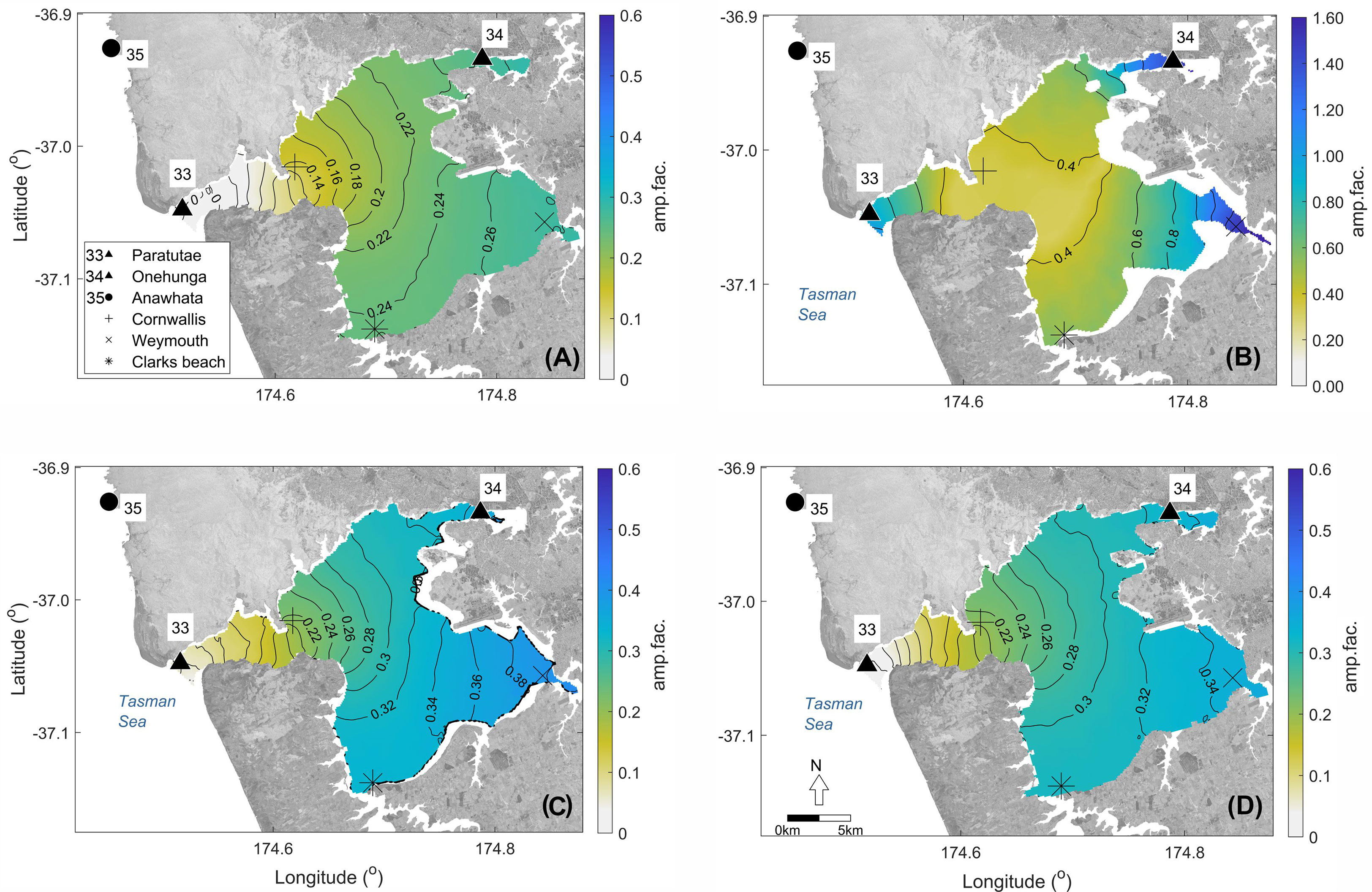
Figure 11 Co-amplification lines of the astronomical tide (A), NTR (B), astronomical tide + NTR (C), and SWL (D) according to the outputs of the simulation scenarios SC2, SC3, SC2+SC3, and SC1 respectively. Note the ocean domain to the west has been removed to focus on the estuary. Background image: aerial photos from Land Information New Zealand (LINZ). Projection: WGS84.

Hydrodynamic modelling also showed the amplification was greater or lower if the NTR and tide were allowed to interact (the model was forced with SWL, SC1) versus when they were modelled separately and added together (SC2+SC3). If the combined model provided a different result to the additive model, then the difference in water level inside and outside the estuary might be accounted for by the TSI (see Section 3.5.1). In fact, when SWL is simulated and tides and NTRs interact (SC1), the amplification is lower in comparison to the scenario when astronomical tide and NTR are considered independent (SC2+SC3). For instance, Figure 11C shows an amplification factor of 0.38 at Weymouth when tides and NTRs are simulated independently (SC2+SC3), while Figure 11D shows an amplification factor of 0.34 at the same location when astronomical tide and NTR interact (SC1). TSI decreases the amplification heterogeneously through the harbour and is more evident in the upper estuarine regions. For instance, the SWL at Weymouth is decreased up to -0.04 (-4%) and at Onehunga is -0.02 (-2%). Considering a peak of SWL occurring at Anawhata of 1.64 m (i.e., the 99.8th percentile), the resulting dampening in the SWL because of the non-linear interactions between tide and NTR would be 6 cm and 3 cm for Weymouth and Onehunga, respectively. Note that these differences consider the maximum SWL at each grid cell over the entire period of simulation and that the differences at the peaks of SWL could be larger as shown in Table 3.

In addition, the NTR directly affects the tidal amplification. Figure 12 shows the effect of positive (A) and negative (B) NTRs on the tide. For instance, the outputs of SC7 and SC8 showed that positive NTR (SC7) decreases the tidal amplification by up -5% (Figure 12A). Negative NTR (SC8) can increase the tidal amplification by +5% (Figure 12B). These differences in the tidal amplification are evident in the inner estuarine region (e.g., nearby Onehunga, Weymouth, and Clark beach).

FIGURE 12

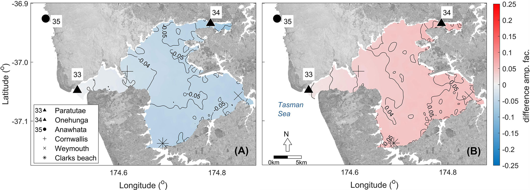
Figure 12 Effects of the NTR on the tidal amplification. The difference in the tidal amplification between a scenario forced by only astronomical tide (SC2) and another forced by astronomical constituents plus a positive (SC7) and a negative (SC8) NTR is shown in panels (A, B), respectively. Note the ocean domain to the west has been removed to focus on the estuary. Background image: aerial photos from Land Information New Zealand (LINZ). Projection: WGS84.

5 Discussion

The astronomical tide and NTR are statistically dependent at most locations of NZ, and the morphology of the coast or estuary can enhance the degree of dependence. This is shown in multiple ways, by analysing the occurrence of the largest NTRs as a function of tide level (i.e., Dixon and Tawn, 1994), tidal phase (i.e., Haigh et al., 2010), and by analysing the dependence between NTRs and astronomical high tide that corresponds to extreme SWLs (i.e., the skew-surge in Arns et al., 2020). The largest NTRs occur at low tide and from 4 to 6 h after the peak of high tide in most of the study sites, especially in the ones located in the inner regions of estuaries.

The degree of dependence between NTR and astronomical tide varied according to the method applied for the analysis. Based on past work, the coasts with a narrow continental shelf, as in NZ, the NTR and astronomical tide were expected to be independent. This assumption is supported here by the results obtained by applying the Dixon and Tawn (1994) method, which showed that TSI did not occur in most of the records from tide gauges located outside estuaries. However, astronomical tide and NTR were shown to be dependent on almost all tide gauges at the coast when the tide phase was used as a basis for analysis (i.e., Haigh et al., 2010) or during extreme SWLs (Arns et al., 2020). There are three possible explanations for this. First, the Haigh et al. method has more degrees of freedom in the chi-squared test than the Dixon and Tawn method, 13 and 5, respectively. Second, the Dixon and Tawn method cannot identify interactions caused by phase alteration, which can be done by Haigh et al. Third, the dependence between NTR and astronomical high tides found during extreme SWLs (i.e., using Arns et al., 2020) may be explained by the lower number of samples (i.e., calculations were made here only using the NTR associated with the highest SWL) and the process of mutual phase alteration. Mutual phase alteration is when tide and surge interact to change each of their propagation celerities — e.g., larger tides (surges) would slow the surge (tide) and consequently decrease the surge (tide) amplitude (Proudman, 1955a; Proudman, 1955b; Rossiter, 1961), see Section 1.

Although a statistical dependence was found between astronomical tides and surges (i.e., for both the NTR and the skew-surge), the magnitude of these interactions can vary widely. For instance, the TSI estimated by applying Arns et al. (2020) showed that the TSI is mostly positive and vary between >+10 cm up to +27 cm. However, these values are averaged for a specific quantile, as TSI for single storms can vary between negative to positive values at the same location (Arns et al., 2020). For instance, the results of our numerical modelling showed that TSI occurs in Manukau Harbour (e.g., Paratutae and Onehunga tidal gauges) and is negative (≅ -16 cm) for a single extreme SWL. That means the SWL would be overestimated if tide and surge were assumed to be independent. In addition, when the difference between the quantiles of skew-surges and NTRs were analysed at the same site (Section 4.1 and 4.2), these differences are close to zero or negative, with the largest of -4 cm and with the skew-surge quantile lower than the respective NTR quantile.

The positive TSI estimated for tide gauges in NZ using the NTR is not what has been observed in most locations globally, using the same methodology (Arns et al., 2020). For instance, Arns et al. (2020) have only observed positive TSI in the Northern Sea. Positive (negative) values of TSI mean that if TSI is not considered, the predictions can be underestimated (overestimated). The positive TSI obtained when applying Arns et al. can be explained by the limitation of statistical models in representing local physical processes, which the author also highlights. For instance, when tide and surges propagate inside an estuary, they interact not just with each other (i.e., mutual phase alteration (Rossiter, 1961)) but also with the geometry, bathymetry, bed friction of the estuary, and local processes that can affect the NTR inside the estuary (as shown with our numerical modelling scenarios). All these factors potentially increase the non-linear response between surges and tides within a harbour, especially in NZ, where the complex morphology and extensive intertidal zones are commonly found in estuaries and are different from the funnel-shaped estuarine settings in pioneering studies of TSI. Another factor which might explain the difference is the lower accuracy of the Arns et al. model on fitting TSI where the astronomical tides represent more than 80% of the SWL during extreme events. Positive TSI was found by the same study for some Pacific islands where the astronomical tide represents >80% of the SWL during extreme events, which is the case of NZ (see Supplementary Table 9). For instance, at Anawhata, Paratutae, and Onehunga tide gauges, the astronomical tide represents ~90% of the SWL during extremes over the 99.8th percentile.

The complex morphology of the estuaries (e.g., extensive intertidal flats) can enhance the TSI because of tide and surge transformations (e.g., asymmetry, amplification, dampening). Usually, the process of mutual phase alteration between astronomical tide and the NTR results in the largest NTRs being unlikely to occur at high tide, but rather within a few hours of high tide, during the rising or falling tide. We show multiple lines of evidence that for NZ’s estuaries with extensive intertidal zones, the largest NTR occurs near the low tide. Firstly, Dixon and Tawn and Haigh et al. methods showed a strong tendency of the largest NTRs to occur close to the low tide and around 4–6 hours after the high tide in estuaries with large intertidal zones (e.g., Onehunga, see Figure 6B). Secondly, a significant correlation that was found between the coefficient τ (NTR × astronomical tide during extreme SWLs) and the area of the intertidal zone throughout the fourteen different estuaries (see Section 4.2). Thirdly, the significant correlation between τ and the M4/M2 was calculated for all 36 tide gauges in this study. Fourthly, our hydrodynamic modelling results showed that water depth and bed friction are equally important for TSI at Manukau Harbour (Section 4.4.1) and can increase or decrease the TSI heterogeneously within the harbour (see Figure 10). Ultimately, the tidal asymmetry and the amplification of shallow-water harmonics result from the effects of bed friction and morphology on the tidal wave propagation, which are the same elements of the shallow-water equations that contribute the most to the TSI. The contribution of bed friction and shallow water effects have been shown as the most important for TSI in previous studies (e.g., Idier et al., 2012; Antony et al., 2020).

In contrast to the relationship between NTR and tides, skew-surges and tides were generally shown to be independent in NZ. In this respect, the Williams et al. and the Arns et al. method (both of which were applied to skew-surge) provide conflicting results, which demonstrates the sensitivity to small differences in how the analysis is performed. Williams et al. method showed that the skew-surges and astronomical tides are independent whereas the Arns et al. method showed that they are dependent. Williams et al. method analyses the dependence between the highest skew-surges and the water level at the nearest astronomical high tide, which can include peaks of SWL occurring during neap and spring tides and results in a larger dataset. The Arns et al. method analyses only the skew-surge and nearest astronomical high tide associated with the highest SWLs (also time-declustered), which results in a much shorter dataset. Williams et al. method was validated for North Atlantic and widely applied globally. Although these regions experience larger NTR than NZ, they also experience larger tides, which makes the contributions of tide and surges to the SWL similar and they are both tide dominant (i.e., NZ and UK) (Williams et al., 2016; Stephens et al., 2020). Most of the coastal flooding studies performed in NZ applied the skew-surge joint probability model (SSJPM), which assumes independence between skew-surge and astronomical tides. Stephens et al. (2020) have compared different methods of extreme value analysis in NZ. In this work, the authors calculated the return period of extreme SWL fitting peaks over threshold using both General-Pareto distribution (GPD) — which theoretically considers the TSI — and the SSJPM. The SSJPM was similar to the GPD or overestimated the return periods of 1 year to 25 years and better fit the return periods >50 years. The overestimation in the lower return periods (i.e.,<50 years) for some of the sites analysed by Stephens et al. (2020) may potentially indicate that the assumption of independence is not always valid — as shown by the tide-skew-surge dependence shown here by the application of Arns et al. method using the highest SWLs. Other studies, such as Santamaria-Aguilar and Vafeidis (2018), have shown that skew-surge and astronomical tide can be dependent, especially in shallow seas (which can apply to estuaries) with mixed semidiurnal tides. In mixed semidiurnal regimes, two high tides occur over a day, but one high tide is lower than the other, which may allow the largest skew-surge to preferably occur at the lower or higher high tide. Although Santamaria-Aguilar and Vafeidis (2018) show convincing evidence that skew-surge and astronomical tide can be dependent, they do state that further numerical modelling should be done to properly prove the dependence. The Santamaria-Aguilar and Vafeidis procedure was also applied to the datasets presented here and no dependence between extreme skew-surge and tides were found (not shown).

The TSI explains the differences in the co-occurrence of extremes inside and outside harbours, which is also supported by the results of the hydrodynamic modelling (Figures 11; 12). First, the model outputs showed that surges can be amplified within the harbour when considering a scenario where NTR are simulated independently and interacting only with the morphology (shallow water effects, bed friction). The NTR amplification is relatively higher than for astronomical tides. Second, TSI was shown to affect the amplification of the astronomical tide. For instance, during an extreme SWL occurring outside the harbour —with an equinoctial high tide and a strong positive NTR (99.8th percentile) — tide and surge would add to each other linearly because the TSI outside the harbour was proven to be weak. However, when the same tide and NTR propagate into the harbour, the tide will be amplified less or more according to the local mean water level, which will vary according to the NTR. In the case of a positive NTR (scenario SC7), the mean water level will be higher, and the tide will propagate more quickly within the estuary. Consequently, the amplification caused by funnelling (due to gradual change of entrance width and bottom friction) or shoaling (due to gradual change of bathymetry) is more likely to decrease, and the corresponding SWL inside the estuary (e.g., at Onehunga tidal gauge) may no longer be considered an extreme event. A practical outcome of these results is that interactions between tide, NTR and morphology would have equal or more impact on the NTR than wind set-up and wind generated waves, which have been shown to increase the water level by few centimetres in Manukau Harbour (Smith et al., 2001).

Although the present study is focused on NZ, the main findings are relevant globally. Although the statistical analyses used here are commonly employed to assess TSI, it can be difficult to interpret the results, particularly when different tests give different outcomes; only a robust numerical study can provide a full physical interpretation of the processes involving tide, NTR, and skew-surge, as highlighted in previous studies (Santamaria-Aguilar and Vafeidis, 2018; Arns et al., 2020). In general, TSI becomes stronger the shallower the bathymetry becomes — e.g., extensive and shallow continental shelf, shallow seas, shallow estuary — and the coastal geometry becomes more complex — e.g., coastal embayment, coastal lagoons — because the shallow water effects, bed friction, and advection enhance non-linear interactions between NTR and tides (Flather, 2001; Zhang et al., 2010). Therefore the results are applicable to similarly complex sites such as the English Channel (Idier et al., 2012), the Southwestern Atlantic coast (Santamaria-Aguilar and Vafeidis, 2018), the Bay of Bengal (Antony et al., 2020), or even the Pacific Islands where Arns et al. have shown that TSI can be positive (as previously discussed). Where TSI is likely to be strong, and in situ water level records are scarce and short, the use of skew-surge joint probability methods is a better approach for robust extreme value analysis (since the skew-surge is less likely to be influenced by TSI). Although in general, extreme skew-surges have been shown to be independent of astronomical tide in most of the locations around the world (Williams et al., 2016), exceptions have been reported (Santamaria-Aguilar and Vafeidis, 2018; Arns et al., 2020). Further validation could use the numerical modelling approach outlined here. Finally, it is generally impractical to adequately monitor a complex coastal setting, and the results here show the limitations on our ability to extrapolate between settings (such as from outside an estuary to inside an estuary). Understanding and being able to isolate morphological effects would help to eventually improve the prediction of non-linear effects and consequently the prediction of extreme water levels inside harbours or in locations with complex geometry. An extreme outside a harbour may not cause extreme event inside the harbour.

A number of processes which may have important effects on tides, NTR, and their dependence on estuarine morphology, have been neglected in this study, such as multiple flooding drivers like wind-generated waves, wind set-up, fluvial discharge, and infragravity waves. For instance, previous studies have shown that wind can generate waves in Manukau Harbour, which can affect the NTR (Smith et al., 2001), especially in estuaries with extensive shallow areas, because the wind stress component of the storm surge is inversely proportional to the water depth (Pugh and Woodworth, 2014). The wind can also induce vertical flows; for instance, return flow in channels, which would be considered by forcing with wind in a 3D hydrodynamic model. The simulation scenarios performed here considered a homogeneous bed friction coefficient over the model domain, which is not realistic; bed materials are not constant throughout the estuary and water depth and current speed can affect them (Sternberg, 1968; Nihoul, 1977; Kagan et al., 2012). However, the model approximated well to the observed amplification in Onehunga, and the general patterns of amplification throughout the estuary corroborates previous studies (Bell et al., 1998). In addition, infragravity and short waves can increase NTR inside estuaries (Bertin et al., 2019). The powerful swells that reach NZ (Godoi et al., 2017; Albuquerque et al., 2021) could produce infragravity waves propagating to inner estuarine regions.

Ultimately, one of the biggest challenges is determining how sea level rise (SLR) is and will affect the TSI in NZ’s estuaries. Although just a few strong trends in skew-surge/SLR and TSI/SLR have been found globally (Mawdsley and Haigh, 2016; Arns et al., 2020), the response of the tidal range and asymmetry to SLR is strongly affected by the estuarine morphology, especially in locations where the tides are the main driver for flooding (Du et al., 2018; Khojasteh et al., 2020; Khojasteh et al., 2021). For instance, Du et al. (2018) have shown that the response of the tidal range to SLR is nonlinear, spatially heterogeneous within the estuary, and highly affected by the length and bathymetry of an estuary, with tidal range decreasing in short estuaries with broad intertidal zones. Khojasteh et al. (2020) have shown that the entrance restriction drives the estuarine response to SLR; the smaller the cross-sectional area of the estuary mouth, the smaller the tidal range within the estuary. Khojasteh et al. (2021), in a broad review on the subject of SLR and its effects on the tidal range in estuaries, concluded that the tidal range is more likely to increase in estuaries where fixed structures (e.g., sea-walls) are established, while in estuaries with preserved intertidal zones and flood-plains, where these areas have space to migrate landward in case of SLR, the tidal range is more likely to decrease.

6 Conclusions

The TSI in observations from 36 tidal gauges around NZ was analysed and a numerical study, focused on a single location (Manukau Harbour), was performed aiming to explain some of the patterns. TSI occurs at most of the sites in NZ and mainly affects the time when the largest surges occur relative to high tide. Furthermore, TSI did not show any regional patterns linked to the distribution of tide, NTR, or skew-surge regimes around NZ. However, the strongest TSI occurs at tide gauges located in inner estuarine locations and are correlated with the intertidal areas within these estuaries. Data analysis, statistical and numerical models were used to quantify the magnitude of the TSI. The values vary according to the method applied, and they are larger for individual events than for quantiles, and range from -16 cm to +27 cm, which means that the water level can decrease (-) or increase (+) if TSI is not accounted for.

In addition, the highest skew-surges and associated astronomical tides were shown to be statistically independent in most cases. This is important because the current return periods of extreme SWL are calculated by using SSJPM which assumes independence between these two variables. In fact, the greater likelihood of independence of the skew-surge (compared to the NTR) is why the skew-surge was used as a basis for the SSJPM. In some cases, skew-surges and astronomical tides were dependent when associated with the highest extreme SWLs (used in the Arns et al. method), which may explain some of the inconsistencies in previous research found in the fitting of extreme value for the lower return period SWLs (up to the 50-year return). Further work is needed to determine the conditions under which skew-surge can be considered unilaterally independent.

Numerical and observational data were used to provide strong evidence that TSI modulates the co-occurrence rate of extreme SWL in estuaries of NZ by affecting tidal amplification. An understanding of the co-occurrence of extreme events is important to develop localised hazard assessment for regional planning. For instance, if observations are available only outside a harbour, the schematisation of the boundary conditions (i.e., waves, tides, surges) being used to drive a hydrodynamic model, may not correspond appropriately to the hydrodynamic response that generates the extreme events inside the harbour. Such an approach would limit understanding of the full range of possible storms affecting the water levels inside estuaries when extreme water levels are estimated using only observations made outside a harbour.

The estuarine morphology has been shown to affect astronomical tide, the NTR and the TSI, as shown by the significant correlation found with the intertidal area. In addition, the ratio between the principal astronomical and the shallow constituent of the astronomical tide and the τ coefficient shows that the importance of the TSI in enclosed sites is likely caused by non-linear effects (which is also supported by the numerical modelling study in Manukau Harbour); however, determining which non-linear term contributes the most to the TSI was not possible (e.g., shallow-water effects, bed friction, or advection terms).

Ultimately, the present manuscript highlights the urgency of investment into tide gauge networks, to provide longer-duration observations inside estuaries and in locations with high morphological complexity. This is particularly important in Aotearoa New Zealand, which has a complex coast in terms of geometry, so tide transformations and their interaction with NTR can generate different local responses to storms than in the open ocean. Ultimately, a better understanding of tide-surge interactions will improve the quality of projections of damage and costs caused by sea level rise and coastal flooding.

Data availability statement

Publicly available datasets were analysed in this study. This data can be found here: https://github.com/CostaAndCoasts/ https://data.linz.govt.nz/ https://envdata.boprc.govt.nz/Data https://www.nrc.govt.nz/environment/environmental-data/environmental-data-hub/ https://waikatoregion.govt.nz/environment/envirohub/ https://www.orc.govt.nz/managing-our-environment/maps-and-data.

Author contributions

The main conception and design of the study were given by WC with important contributions given by KB, SS, and GC. The statistical analysis and numerical modelling were performed by WC and supervised by KB and SS. The database was organised by SS and WC. The first draft of the manuscript was written by WC. All authors contributed to manuscript revision, read, and approved the submitted version.

Funding

This work was supported by the National Science Challenge: Resilience Challenge “Coasts” programme, GNS-RNC040.

Conflict of interest

Author SS was employed by National Institute for Water and Atmospheric Research Ltd.

The remaining authors declare that the research was conducted in the absence of any commercial or financial relationships that could be construed as a potential conflict of interest.

Publisher’s note

All claims expressed in this article are solely those of the authors and do not necessarily represent those of their affiliated organizations, or those of the publisher, the editors and the reviewers. Any product that may be evaluated in this article, or claim that may be made by its manufacturer, is not guaranteed or endorsed by the publisher.

Supplementary material

The Supplementary Material for this article can be found online at: https://www.frontiersin.org/articles/10.3389/fmars.2023.1170756/full#supplementary-material

References

Albuquerque J., Antolínez J. A. A., Gorman R. M., Méndez F. J., Coco G. (2021). Seas and swells throughout New Zealand : a new partitioned hindcast. Ocean Model. 168, 101897. doi: 10.1016/j.ocemod.2021.101897

CrossRef Full Text | Google Scholar

Antony C., Unnikrishnan A. S., Krien Y., Murty P. L. N., Samiksha S. V., Islam A. K. M. S. (2020). Tide–surge interaction at the head of the bay of Bengal during cyclone aila. Reg. Stud. Mar. Sci. 35, 101133. doi: 10.1016/j.rsma.2020.101133

CrossRef Full Text | Google Scholar

Arns A., Wahl T., Wolff C., Vafeidis A. T., Haigh I. D., Woodworth P., et al. (2020). Non-linear interaction modulates global extreme sea levels, coastal flood exposure, and impacts. Nat. Commun. 11, 1–9. doi: 10.1038/s41467-020-15752-5

PubMed Abstract | CrossRef Full Text | Google Scholar

Batstone C., Lawless M., Tawn J., Horsburgh K., Blackman D., McMillan A., et al. (2013). A UK best- practice approach for extreme sea-level analysis along complex topographic coastlines. Ocean Eng. 71, 28–39. doi: 10.1016/j.oceaneng.2013.02.003

CrossRef Full Text | Google Scholar

Beavan R. J., Litchfield N. J. (2012) Vertical land movement around the New Zealand coastline: implications for sea-level rise, GNS science report 2012/29. Available at: https://www.hbrc.govt.nz/assets/Hazards-Database/Sea-level-rise-projections-adjusted-for-vertical-tectonic-land-movement-along-the-Hawkes-Bay-coastline.pdf.

Google Scholar

Bell R. G., Dumnov S. V., Williams B. L., Greig M. J. N. (1998). Hydrodynamics of manukau harbour, New Zealand. New Zeal. J. Mar. Freshw. Res. 32, 81–100. doi: 10.1080/00288330.1998.9516807

CrossRef Full Text | Google Scholar

Bell R., Hannah J., Andrews C. (2022). Update to 2020 of the annual mean sea level series and trends around New Zealand. Prepared Ministry Environ. August 2022 (NIWA Client Rep. No: 2021236HN) (New Zealand: NIWA). Available at: https://environment.govt.nz/publications/update-to-2020-of-the-annual-mean-sea-level-series-and-trends-around-new-zealand.

Google Scholar

Bernier N. B., Thompson K. R. (2007). Tide-surge interaction off the east coast of Canada and the northeastern united states (C06008: J. Geophys. Res. 112). doi: 10.1029/2006JC003793

CrossRef Full Text | Google Scholar

Bertin X., Mendes D., Martins K., Fortunato A. B., Lavaud L. (2019). The closure of a shallow tidal inlet promoted by infragravity waves. Geophys. Res. Lett. 46, 6804–6810. doi: 10.1029/2019GL083527

CrossRef Full Text | Google Scholar

Codiga D. L. (2011). Unified tidal analysis and prediction using the UTide Matlab functions. Univ. Rhode Island Tech. Rep. no: URI/GSO Tech. Rep. 2011-01. doi: 10.13140/RG.2.1.3761.2008

CrossRef Full Text | Google Scholar

Coles S. (2001). An introduction to statistical modeling of extreme values (London, New York: Springer).

Google Scholar

Dixon M. J., Tawn J. A. (1994). Extreme Sea-levels at the UK a-class sites: site–by-site analysis. Pol. Internal Document no 65. Available at: http://www.pol.ac.uk/ntslf/pdf/id65.pdf.

Google Scholar

Doodson A. T. (1929). Report on Thames floods. Geophys. Mem. Lond. 47, 1–26. https://searchworks.stanford.edu/view/133937.

Google Scholar

Du J., Shen J., Zhang Y. J., Ye F., Liu Z., Wang Z., et al. (2018). Tidal response to Sea-level rise in different types of estuaries: the importance of length, bathymetry, and geometry. Geophys. Res. Lett. 45, 227–235. doi: 10.1002/2017GL075963

CrossRef Full Text | Google Scholar

Flather R. A. (2001). “Storm surges”. Encyclopedia Ocean Sci. (San Diego, California: Academic Press), 2882–2892. doi: 10.1006/rwos.2001.0124

CrossRef Full Text | Google Scholar

Godoi V., Bryan K. R., Stephens S. A., Gorman R. M. (2017). Extreme waves in New Zealand waters. Ocean Model. 117, 97–110. doi: 10.1016/J.OCEMOD.2017.08.004

CrossRef Full Text | Google Scholar

Haigh I., Nicholls R., Wells N. (2010). Assessing changes in extreme sea levels: application to the English channe-2006. Cont. Shelf Res. 9, 1042–1055. doi: 10.1016/J.CSR.2010.02.002

CrossRef Full Text | Google Scholar

Horsburgh K. J., Wilson C. (2007). Tide-surge interaction and its role in the distribution of surge residuals in the north Sea. J. Geophys. Res. 112, C08003. doi: 10.1029/2006JC004033

CrossRef Full Text | Google Scholar

Hume T., Gerbeaux P., Hart D., Kettles H., Neale D. (2016). A classification of New Zealand’s coastal hydrosystems. Prepared Ministry Environment. October (NIWA Client Rep. No: HAM2016-062) (New Zealand NIWA). Available at: https://environment.govt.nz/publications/a-classification-of-new-zealands-coastal-hydrosystems/.

Google Scholar

Idier D., Dumas F., Muller H. (2012). Tide-surge interaction in the English channel. Nat. Hazards Earth Syst. Sci. 12, 3709–3718. doi: 10.5194/nhess-12-3709-2012

CrossRef Full Text | Google Scholar

Jane R., Wahl T., Santos V. M., Misra S. K., White K. D. (2022). Assessing the potential for compound storm surge and extreme river discharge events at the catchment scale with statistical models: sensitivity analysis and recommendations for best practice. J. Hydrol. Eng. 27, 1–16. doi: 10.1061/(asce)he.1943-5584.0002154

CrossRef Full Text | Google Scholar

Kagan B. A., Sofina E. V., Rashidi E. (2012). The impact of the spatial variability in bottom roughness on tidal dynamics and energetics, a case study: the m 2 surface tide in the north European basin. Ocean Dyn. 62, 1425–1442. doi: 10.1007/s10236-012-0571-3

CrossRef Full Text | Google Scholar

Kendall M. G. (1938). A new measure of rank correlation. Biometrika 30 (1–2), 81–93. doi: 10.1093/biomet/30.1-2.81

CrossRef Full Text | Google Scholar

Khojasteh D., Glamore W., Heimhuber V., Felder S. (2021). Sea level rise impacts Estuar. dynamics: A review. Sci. Total Environ. 780, 146470. doi: 10.1016/j.scitotenv.2021.146470

CrossRef Full Text | Google Scholar

Khojasteh D., Hottinger S., Felder S., De Cesare G., Heimhuber V., Hanslow D. J., et al. (2020). Estuarine tidal response to sea level rise: the significance of entrance restriction. Estuar. Coast. Shelf Sci. 244, 106941. doi: 10.1016/j.ecss.2020.106941

CrossRef Full Text | Google Scholar

Liu W. C., Huang W. C., Chen W. B. (2016). Modeling the interaction between tides and storm surges for the Taiwan coast. Environ. Fluid Mech. 16, 721. doi: 10.1007/s10652-015-9441-0

CrossRef Full Text | Google Scholar

Mawdsley R. J., Haigh I. D. (2016). Spatial and temporal variability and long-term trends in skew surges globally. Front. Mar. Sci. 3. doi: 10.3389/fmars.2016.00029

CrossRef Full Text | Google Scholar

Naderi A., Siadatmousavi S. M. (2023). Extreme value analysis for waves in the Persian gulf: skill assessment of different methods for a fetch-limited basin, reg. Stud. Mar. Sci. 59, 102812. doi: 10.1016/j.rsma.2023.102812

CrossRef Full Text | Google Scholar

Nasr A. A., Wahl T., Rashid M. M., Camus P., Haigh I. D. (2021). Assessing the dependence structure between oceanographic, fluvial, and pluvial flooding drivers along the united states coastline. Hydrol. Earth Syst. Sci. 25, 6203–6222. doi: 10.5194/hess-25-6203-2021

CrossRef Full Text | Google Scholar

Nihoul J. C. J. (1977). Three-dimensional model of tides and storm surges in a shallow well-mixed continental sea. Dyn. Atm. Oceans 2, 29–47. doi: 10.1016/0377-0265(77)90014-8

CrossRef Full Text | Google Scholar

Oppenheimer M., Glavovic B. C., Hinkel J. R., van de Wal R., Magnan A. K., Abd-Elgawad A., et al. (2019). Sea Level rise and implications for low-lying islands, coasts and communities. IPCC Special Rep. Ocean Cryosphere Changing Climate Pö̈rtner H.-O., Roberts D.C., Masson-Delmotte V., Zhai P., Tignor M., Poloczanska E., et al. (Cambridge, UK and New York, NY, USA: Cambridge University Press), 321–445. doi: 10.1017/9781009157964.006

CrossRef Full Text | Google Scholar

Orton P., Georgas N., Blumberg A., Pullen J. (2012). Detailed modeling of recent severe storm tides in estuaries of the new York city region. J. Geophys. Res.-Oceans 117, C09030. doi: 10.1029/2012jc008220

CrossRef Full Text | Google Scholar

Park Y. H., Suh K. (2012). Variations of storm surge caused by shallow water depths and extreme tidal ranges. Ocean Eng. 55, 44–51. doi: 10.1016/j.oceaneng.2012.07.032

CrossRef Full Text | Google Scholar

Plüß A., Rudolph E., Schrodter D. (2001). Characteristics of storm surges in German estuaries. Clim. Res. 18, 71–76. doi: 10.3354/cr018071

CrossRef Full Text | Google Scholar

Proudman J. (1955a). The effect of friction on a progressive wave of tide and surge in an estuary. Proc. R. Soc Lond. A 233, 407–418.

Google Scholar

Proudman J. (1955b). The propagation of tide and surge in an estuary. Proc. R. Soc Lond. A. 231, 8–24.

Google Scholar

Pugh D., Woodworth P. (2014). Sea-Level science: understanding tides, surges, tsunamis and mean Sea-level changes (Cambridge: Cambridge University Press). doi: 10.1017/CBO9781139235778

CrossRef Full Text | Google Scholar

Rego J. L., Li C. (2010). Storm surge propagation in Galveston bay during hurricane Ike. J. Mar. Syst. 82, 265–279. doi: 10.1016/j.jmarsys.2010.06.001

CrossRef Full Text | Google Scholar

Rossiter J. R. (1961). Interaction between tide and surge in the Thames. Geophys. J. Int. 6, 29–53. doi: 10.1111/j.1365-246X.1961.tb02960.x

CrossRef Full Text | Google Scholar

Rueda A., Cagigal L., Antolínez J. A. A., Albuquerque J. C., Castanedo S., Coco G., et al. (2019). Marine climate variability based on weather patterns for a complicated island setting: the New Zealand case. Int. J. Climatol. 39, 1777–1786. doi: 10.1002/joc.5912

CrossRef Full Text | Google Scholar

Santamaria-Aguilar S., Vafeidis A. T. (2018). Are extreme skew surges independent of high water levels in a mixed semidiurnal tidal regime? J. Geophys. Res. Ocean. 123, 8877–8886. doi: 10.1029/2018JC014282

CrossRef Full Text | Google Scholar

Santos V. M., Wahl T., Jane R., Misra S. K., White K. D. (2021). Assessing compound flooding potential with multivariate statistical models in a complex estuarine system under data constraints. J. Flood Risk Manage. 14, 1–16. doi: 10.1111/jfr3.12749

CrossRef Full Text | Google Scholar

Scarrott C., MacDonald A. (2012). A review of extreme value threshold estimation and uncertainty quantification. Revstat Stat. J. 10 (1), 33 –60. doi: 10.57805/revstat.v10i1.110

CrossRef Full Text | Google Scholar

Smith M. J., Stevens C. L., Gorman R. M., McGregor J. A., Neilson C. G. (2001). Wind-wave development across a large shallow intertidal estuary: a case study of manukau harbour, New Zealand. New Zeal. J. Mar. Freshw. Res. 35, 985–1000. doi: 10.1080/00288330.2001.9517058

CrossRef Full Text | Google Scholar

Speer P. E., Aubrey D. G. (1985). A study of non-linear tidal propagation in shallow inlet-estuarine systems. part II: theory. Est. Coast. Shelf Sci. 21, 207–224. doi: 10.1016/0272-7714(85)90097-6

CrossRef Full Text | Google Scholar

Stephens S. A., Bell R. G., Haigh I. D. (2020). Spatial and temporal analysis of extreme storm-tide and skew-surge events around the coastline of New Zealand. Nat. Hazards Earth Syst. Sci. 20, 783–796. doi: 10.5194/nhess-20-783-2020

CrossRef Full Text | Google Scholar

Sternberg R. W. (1968). Friction factors in tidal channels with differing bed roughness. Mar Geol. 6, 243–260. doi: 10.1016/0025-3227(68)90033-9

CrossRef Full Text | Google Scholar

Tadesse M. G., Wahl T. (2021). A database of global storm surge reconstructions. Sci. Data 8, 1–10. doi: 10.1038/s41597-021-00906-x

PubMed Abstract | CrossRef Full Text | Google Scholar

Tang Y. M., Grimshaw R., Sanderson B., Holland G. (1996). A numerical study of storm surges and tides with application to the north Queensland coast. J. Phys. Oceanogr. 26, 2700–2711. doi: 10.1175/1520-0485

CrossRef Full Text | Google Scholar

van Rijn L. C. (2011). Analytical and numerical analysis of tides and salinities in estuaries; part I: tidal wave propagation in convergent estuaries. Ocean Dyn. 61, 1719–1741. doi: 10.1007/s10236-011-0453-0

CrossRef Full Text | Google Scholar

Vousdoukas M. I., Breyiannis G., Feyen L., Salamon P., Ciavola P., Voukouvalas E., et al. (2019). Towards robust pan-European storm surge forecasting. Ocean Model. 133, 129–144. doi: 10.1016/j.ocemod.2018.12.001

CrossRef Full Text | Google Scholar

Williams J., Horsburgh K. J., Proctor R. N. F. (2016). Tide and skew surge independence: new insights for flood risk. Geophys. Res. Lett. 43, 6410–6417.

Google Scholar

Wolf J. (1981). Surge-tide interaction in the north Sea and river Thames. Floods Due to High Winds Tides (New York, NY: Elsevier) 75–94.

Google Scholar

Zhang H., Cheng W., Qiu X., Feng X., Gong W. (2017). Tide-surge interaction along the east coast of the leizhou peninsula, south China Sea. Cont. Shelf Res. 142, 32–49. doi: 10.1016/j.csr.2017.05.015

CrossRef Full Text | Google Scholar

Zhang W. Z., Shi F., Hong H.-S., Shang S.-P., Kirby J. T. (2010). Tide-surge interaction intensified by the Taiwan strait. J. Geophys. Res. 115, C06012. doi: 10.1029/2009JC005762

CrossRef Full Text | Google Scholar