Deoxygenation of the Baltic Sea during the last millennium

1 Introduction

Deoxygenation and low-oxygen conditions have been well-documented in coastal waters and the open ocean since the middle of the 20th century (Breitburg et al., 2018). Increasing hypoxia (<2mg/l O₂) has altered the abundance and distribution ofmarine species globally but has mostly affected coastal seas (Breitburg et al., 2018). During the last century, the rise of hypoxia in the Baltic Sea was mainly associated with eutrophication caused by an increased discharge of nutrients from land (Gustafsson et al., 2012; Meier et al., 2019a) and is thus anthropogenically induced. To counteract eutrophication, land-based phosphorus discharge has decreased since the 1980s. However, eutrophication still increased, likely linked to an internal phosphorus loading from anoxic bottoms [e.g. Mortimer, 1942] providing a positive feedback mechanism that may explain the increase of the phosphorus concentration in the surface layer in winter in the Baltic proper (Stigebrandt and Andersson, 2020).

The semi-enclosed Baltic Sea (Figure 1) is naturally prone to hypoxic conditions. The limited exchange with the open ocean creates a strong stratification, restricting the ventilation of deep waters from above [e.g (Conley et al., 2002; Savchuk, 2018)]. Hence, oxygen is mainly supplied by a lateral inflow of dense, saline, and oxygenated water from the North Sea surface waters that flows below the permanent halocline. Inflow events renew deep waters but also prohibit further ventilation by strengthening stratification (Conley et al., 2009). During windier conditions, enhanced vertical mixing can transport well-oxygenated surface waters across the halocline, affecting the upper deep waters (80-125 m) (Conley et al., 2009).

FIGURE 1

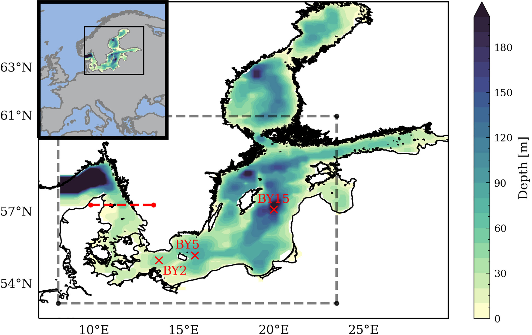
Figure 1 Bottom topography of the Baltic Sea used in the ocean model, including Kattegat and Skagerrak. The domain for the analysis follows Krapf et al. (2022) (dashed grey line). For the comparison with Schimanke et al. (2012), the domain was adjusted as their open boundary is limited in the northern Kattegat (dashed red line). Moreover, the location of the stations BY2 (Arkona Basin), BY5 (Bornholm Basin), and BY15 (Gotland Deep) are shown.

In recent years, the Baltic Sea contained one of the world’s largest hypoxic areas (Almroth-Rosell et al., 2011; Fennel and Testa, 2019; Krapf et al., 2022). However, sediment records have shown that the Baltic Sea also experienced hypoxic episodes before the industrial revolution. The warm medieval climate anomaly (MCA; 950 - 1250 C.E (Mann et al., 2009).) coincided with increasing hypoxia in the Baltic Sea (Zillén et al., 2008). Following the MCA, a global cooling trend during the Little Ice Age [LIA; ca. 1350-1700 C.E; 12] coincided with a decline in hypoxic area (Zillén et al., 2008).

A key role of the intensifying anoxic conditions is attributed to a positive feedback mechanism (Vahtera et al., 2007; Funkey et al., 2014): The onset of bottom-water anoxia leads to the rapid reduction of iron oxide and the release of iron-bound phosphorus in surficial sediments, which increases the availability of in phosphate in the water-column (Mortimer, 1942; Ingall et al., 1993). This may enhance cyanobacteria’s nitrogen fixation and increase the available nitrogen for other phytoplankton species (Vahtera et al., 2007; Savchuk, 2018; Meier et al., 2019a). The sedimentary iron-bound phosphate inventory and long residence of phosphorus in the Baltic Sea can sustain eutrophication for decades (Conley et al., 2002; Radtke et al., 2012).

Generally, primary production in large parts of the Baltic Sea is nitrogen-limited during spring and early summer. However, cyanobacteria that can fixate atmospheric nitrogen depend only on phosphorus availability and may bloom later in summer. In the Baltic Sea, cyanobacteria blooms only appear to occur at mild weather conditions and temperatures above 16°C (Wasmund, 1997). Consequently, cyanobacteria have been proposed to drive the spreading of hypoxia during the warmer MCA, amplified by the additional phosphorus released from the sediment (Kabel et al., 2012; Funkey et al., 2014; Warden et al., 2017; Kahru et al., 2020).

Besides the temperature-dependent response of the ecosystem, very large saltwater inflows also impact the salinity stratification in the water column and might ultimately lead to anoxia, with only a small contribution of the organic matter (Stigebrandt and Andersson, 2020). Stigebrandt and Andersson (2020) argued that a period of anoxia might be ended by a long period with nearly no saltwater inflow, leading to halocline deepening and, eventually, a vanishing volume of deepwater. Thus, both the onset and the ending of periods of deepwater anoxia in the Baltic Sea may depend on extreme sequences of saltwater inflow. Still, identifying a physical mechanism that drove the increase in hypoxia during the last millennium has been challenging so far (Schimanke et al., 2012; Giesse et al., 2020; Moros et al., 2020).

Model studies focusing on centennial hypoxia variability in the Baltic Sea are rare: Hansson and Gustafsson (2011) investigated the evolution of salinity and hypoxia since 1500 AD. They found that the average salinity increased by 0.5 g/kg since 1500 with a maximum around 1750. Their results suggest that lower salinity is associated with better ventilation in the upper deep water, while higher salinity is associated with more oxygen in the lower deep water. Hence, oxygen levels in deeper parts of the Baltic Sea improved during the LIA. Schimanke et al. (2012) were the first to perform a dynamical downscaling of a global circulation model for the Eurocordex region, covering the full MCA and LIA from 950 to 1800. However, they could not simulate the entire period from 950 to 1800 due to computational costs. In their work, they simulated 100-year slices of the MCA and the LIA using a coupled ocean-biogeochemistry model (RCO-SCOBI). They could neither simulate anoxic or hypoxic conditions nor link salinity or temperature anomalies to hypoxia during the MCA. However, they found a weak temperature response with slightly reduced oxygen concentrations during the MCA compared to the LIA, with a maximum difference of 0.5 ml/l.

One open question is the actual temperature anomaly during the MCA. Multiple sedimentary proxies (TEX₈₆ records) show an increase of 2 °C (Kabel et al., 2012) whereas Schimanke et al. (2012) estimated an average increase of about 0.4 °C, mostly caused by warmer winters. Schimanke et al. (2012) also increased the air temperature by 2 °C from 1200 to 1299 in their model but still could not reproduce hypoxic conditions in the Baltic Sea deep water, evident from sedimentological studies [e.g. 27]. In contrast, artificially increasing the nutrient loads increased the oxygen difference between the MCA and the LIA.

Studies of Zillén et al. (2008) and Zillen and Conley (2010) proposed that the growth of the surrounding population and their agriculture during the MCA may have increased the nutrient loads and, thereby, the hypoxic area. However, these conclusions are challenged by empirical studies finding no evidence that hypoxia in the open Baltic Sea during the Medieval Climate Anomaly was caused by human activities on land (Jokinen et al., 2018; Ning et al., 2018; Norbäck Ivarsson et al., 2019; van Helmond et al., 2020). In addition, other modeling studies such as Kabel et al. (2012) argued for a temperature-dependent hypoxia response during the MCA. They simulated the Modern Warm Period (MoWP; since 1850) and a delta-approach-based period similar to the LIA, resulting in a temperature difference of approximately 2°C, allowing them to connect the role of a warming climate during the MCA to strengthening cyanobacteria blooms leading to increased hypoxia. Pigment analysis supports the hypothesis of increased cyanobacterial blooms during the MCA (Warden et al., 2017).

In this study, we conduct a simulation covering the entire MCA and LIA from 950 to 1800 using a three-dimensional circulation model with an integrated biogeochemical model using the atmospheric fields from Schimanke et al. (2012). We address the role of natural temperature fluctuations for oxygen conditions in the Baltic Sea and focus on the temperature-related processes that drive hypoxia formation on multidecadal time scales. We conduct three additional sensitivity experiments with enhanced temperatures during the MCA and colder conditions during LIA and two experiments with dedicated temperature manipulation in selected biogeochemical processes. In our analysis, we investigate the role of the positive phosphorus feedback loop due to anoxic conditions and the temperature dependence of the mineralization rate, as both processes contribute to the formation of hypoxia.

2 Data and methods

2.1 Coupled biogeochemical and circulation model

We use a coupled system of circulation and biogeochemical model similar to Neumann et al. (2022). The circulation model is the Modular Ocean Model (MOM5.1) (Griffies, 2004) adapted for the Baltic Sea (Figure 1). The horizontal resolution is 8 nautical miles. Vertically, the model is resolved into 100 layers with a layer thickness of 0.5 m at the surface and gradually increasing with depth up to 2 m.

The circulation model has an integrated sea ice model (Winton, 2000) accounting for ice formation, and the sea ice dynamics are based on Hunke and Dukowicz (1997). The biogeochemical model ERGOM is coupled with the circulation model via the tracer module, which is part of the MOM5.1 code. We decided for the relatively coarse resolution as a trade-off between simulation costs and model quality (see Sec. 2.4).

The ERGOM (Neumann et al., 2022) describes nitrogen, phosphorus, carbon, oxygen, and partly sulfur cycles. Primary production, forced by photosynthetically active radiation (PAR), is provided by three functional phytoplankton groups (large cells, small cells, and cyanobacteria). The chlorophyll concentration in the optical model is estimated from the phytoplankton groups (Neumann et al., 2021). Dead organic matter accumulates in the detritus state variable. Bulk zooplankton grazes on phytoplankton and is the highest trophic level considered in the model. Phytoplankton and detritus can sink into the water column and accumulate in a sediment layer. Detritus is mineralized into dissolved inorganic nitrogen and phosphorus in the water column and the sediment. Mineralization is controlled by water temperature and oxygen concentration. Under oxic conditions, phosphate binds iron oxide and is retained as particles in the sediments. Erosion events can resuspend these particles, and currents transport them toward the accumulation bottom. Under anoxic conditions, iron–oxide becomes reduced, and phosphate is liberated and available as dissolved phosphate. A detailed description of how this process is implemented is given in Neumann and Schernewski (2008). Oxygen is produced by primary production and consumed due to all other processes, e.g., metabolism and mineralization. Extracellular excretion of dissolved organic matter by phytoplankton can induce non-redfieldian carbon uptake. A detailed description of the model is given in Neumann et al. (2022).

This study evaluates the importance of temperature-dependent biogeochemical processes for oxygen dynamics. For this purpose, we introduce a method in the model code that allows us to manipulate temperature-sensitive biogeochemical processes.

2.2 Model setup and forcing

2.2.1 Atmospheric forcing of the ocean model

The atmospheric fields are based on the results of Schimanke et al. (2012). They performed a dynamical downscaling of a multi-centennial paleoclimate simulation using the regional circulation model Rossby Centre Atmosphere Model (RCA3) (Samuelsson et al., 2011). The downscaling covers the period 950 to 1800. The model region is the EURO-CORDEX domain, which ranges from Northern Africa to Northern Scandinavia (33.0°W to 58.52°E; 26.0°N to 71.76°N). At the lateral boundaries, RCA3 was forced by the global circulation model ECHO-G (Hünicke et al., 2010). RCA3 has a horizontal resolution of 0.44° x 0.44°, consists of 24 vertical levels, and has a 30-minute time step. The model provides 10 m winds, 2-m air temperature, 2 m specific humidity, precipitation, total cloudiness, and sea level pressure.

The downward longwave radiation is computed from cloudiness, air temperature, and specific humidity. The calculation follows Berliand and Berliand (1952) with an adjustment of the cloud coverage.

$\begin{array}{ll}{Q}_H\downarrow =Cϵ\sigma T_a^4·(0.39-0.05e_a^{1/2})& (1)\end{array}$

with $e_a=\frac{q·p_{air}}{0.622}$, C = 1 - 0.8 $·cf$, $cf=$ cloudiness, $Q_H$ = downward longwave radiation, $C$ = cloud correction, $ϵ$ = emissivity of water, $\sigma$ = Boltzmann constant, $T_a$ = air temperature, $e_a$ = vapor pressure, $q$ = specific humidity, $p_{air}$ = air pressure.

The upward longwave radiation is calculated by the ocean model using black-body radiation. The resulting net longwave radiation is responsible for the transfer of heat.

The solar radiation follows mainly Bodin (1979) and is modified by Meier et al. (1999). The radiation at the sea surface is described as

$\begin{array}{ll}{S}_{sol}=(1-\alpha )Q_0{T}_{u}s(Tr-Ab)(1-cf),& (2)\end{array}$

with $Tr$ and $Ab$ as transmissivity and absorption. $T_u$ is defined as the transmissivity of the upper atmosphere, $\alpha$ as albedo, s as the zenith angle, and $Q_0$ as the solar radiation at the upper atmosphere.

$Tr$ and $Ab$ are defined as:

$$Tr=1.041-\frac{0.16}{\sqrt{s}}$$

$$Ab=0.077{\left(\frac{\tau }{s}\right)}^{0.3}$$

$\tau$ is the optical path length and is given by:

$$\tau =1.25+0.75\sin \left(2\pi \frac{d-120}{365.25}\right),$$

with $d$ as the day of the corresponding year.

2.2.2 Runoff

The monthly river inputs from 950 to 1800 have been extracted from (Schimanke and Meier, 2016). However, in contrast to the 31 rivers used in their simulation, we first accumulated the basin-wide river runoff and then redistributed it across the 79 rivers used in our model setup. For the nutrient inputs, we used 90% of the pre-industrial levels as defined in (Gustafsson et al., 2012). Riverine inputs of nutrients into the model are interpreted as concentrations. Hence, the nutrient input into the Baltic Sea is scaled by the river runoff of the respective river.

2.2.3 Model experiments

Six sensitivity experiments were performed to investigate the impact of temperature changes on the deoxygenation of the Baltic Sea (Table 1). Similar to Schimanke et al. (2012) we treat the first 100 years as spin-up. The initial conditions for all models are based on a full integration of the model over the period 950 to 1800.

TABLE 1

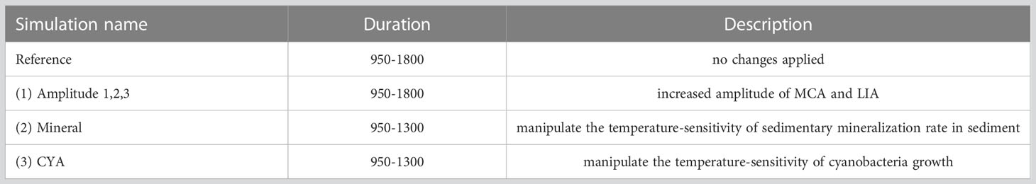
Table 1 Overview of performed model simulations.

(1) Amplitude experiments 1-3 represent different warming (cooling) scenarios for the MCA (LIA) by changing the surface air temperature. We calculated the spatially averaged surface air temperature over the Baltic Sea region (1). In the following, we applied a 4-year running mean as a low-pass filter and calculated the anomaly. The resulting signal was then scaled by the factors 1.5, 2, and 3 and added to the original time series for every grid cell and time step. The resulting mean surface air temperature for the scenarios Amplitude 1, 2, and 3 is shown in Figure 2. The temperature difference between the MCA and the LIA is heavily debated in the literature and ranges from 0.6°C to 2°C. Hence, the applied temperature change remains in the range of possible scenarios.

FIGURE 2

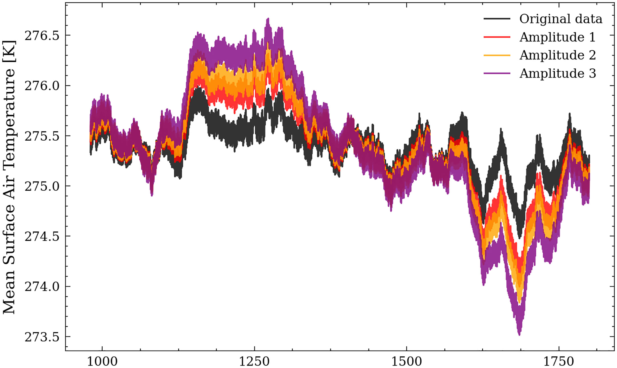
Figure 2 Mean surface air temperature over the Baltic Sea region for the scenarios Amplitude 1,2, and 3.

After changing the air temperature, we corrected the specific humidity using the Clausius-Clapeyron relationship.

(2) The Mineral experiment increased the temperature of the mineralization rate in the sediment (only in the ecosystem model) by 20% (when given in °C), which corresponds to an average increase of 1.2°C. We decided to change only the sediment mineralization rate, as it has been identified as the main driver of mineralization (Schneider et al., 2010).

(3) The CYA experiment increased the temperature in processes relevant to cyanobacteria growth by 7.5%. This corresponds to roughly the same temperature increase as applied in the Mineral experiment.

Note that the water temperature in (2) and (3) is not modified, but the model only artificially increases the input temperature for the selected processes. This approach allows the sensitivity of the respective biogeochemical processes of experiments (2) and (3) to be evaluated without changing circulation patterns in the model, which might be driven by baroclinic gradients related to temperature changes.

2.3 Apparent oxygen utilization

Oxygen concentration in the ocean is controlled by air-sea flux, solubility, and oxygen-producing and consuming biogeochemical processes. We are interested in the impact of the biogeochemical processes on oxygen dynamics. Therefore, we virtually excluded the solubility effect by using the apparent oxygen utilization (AOU), which describes the difference between oxygen saturation concentration and ambient oxygen concentration, including oxygen equivalents of hydrogen sulfide [e.g (Garcia et al., 2005)].

$$AOU=O_2(solubility)-O_2(observed)$$

2.4 Validation of the model

To evaluate our model setup, we simulated the period 1948 – 2018 and compared the resulting model data to observational data from the ODIN2 database. The model was forced with the CoastDat2 reanalysis data (Geyer and Rockel, 2013; Geyer, 2014). River runoff and nutrient loads are based on HELCOM data (HELCOM, 2018). The initial conditions were taken from a hindcast simulation that started in 1850 (Placke et al., 2021).

Modeled and observed time series of surface and bottom salinity (Figure 3), as well as surface phosphate, surface nitrate (Figure 4), bottom phosphate (Figure 5), and bottom oxygen concentration (Figure 6), are compared for station BY15 in the Eastern Gotland Basin in the central Baltic Sea (Figure 1). Further stations (BY2 and BY5) can be found in the supplements.

FIGURE 3

Figure 3 Surface and bottom salinity in the central Baltic Sea (Gotland Deep, BY15).

FIGURE 4

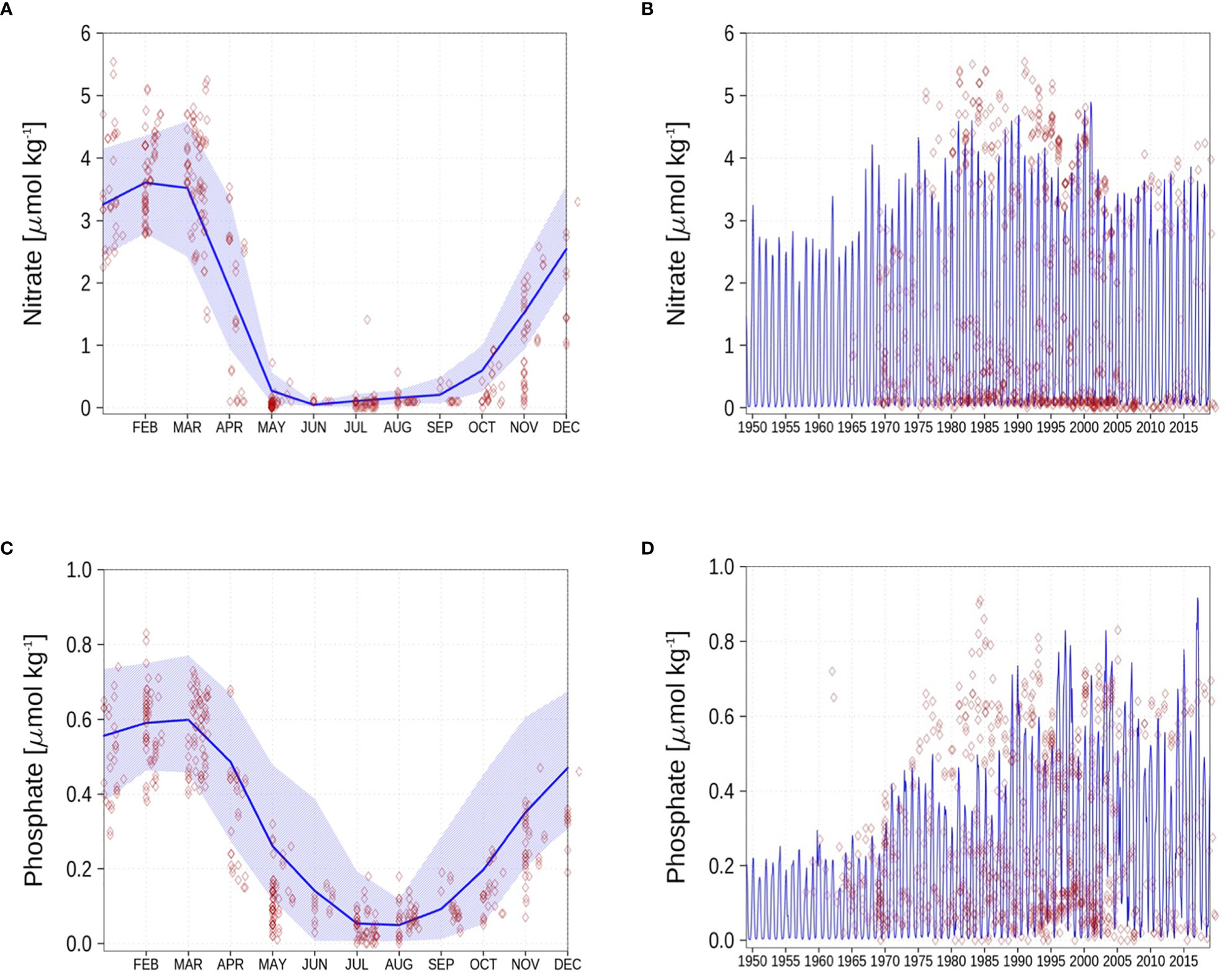
Figure 4 Surface nutrients concentrations at station BY15. Blue color are model simulations, and observations are shown as red diamonds. The blue-shaded area is in the range between the 10th and 90th percentile of model results. The opacity of the red diamonds reflects the frequency of observations. (A): Nitrate climatology, (B): Nitrate time series, (C): Phosphate climatology, (D): Phosphate time series.

FIGURE 5

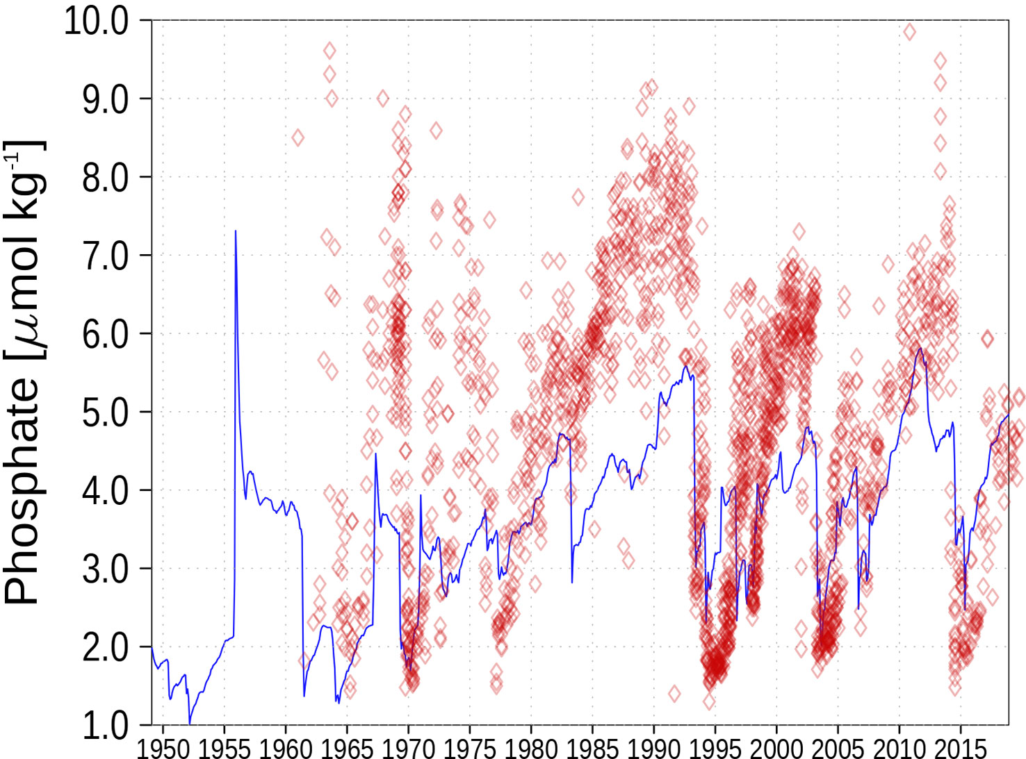
Figure 5 Bottom phosphate concentration at station BY15. Blue color are model simulations and observations are shown as red diamonds.

FIGURE 6

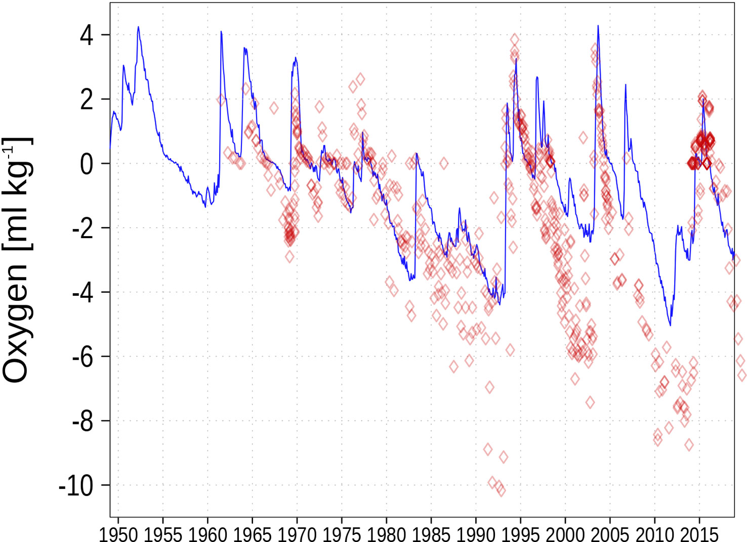
Figure 6 Bottom oxygen concentration in the central Baltic Sea (Gotland Deep; BY15).

The model shows small biases in surface salinity and underestimates bottom salinity at BY15 by about 1 g/kg (Figure 3). Figure 3B shows that peak salinity values after inflows are unrealistically low, but the temporal trends of salinity decrease during stagnation periods appear realistic. This suggests that the excess mixing mostly happens as entrainment into the inflow plume and not permanently. Stronger entrainment of ambient water is possibly due to the z*-level coordinates of the model preventing a direct advective transport between adjacent bottom water cells of different depth. The diapycnal mixing itself could be too strong as well (Burchard and Rennau, 2008). Still, the interannual variability is comparable. This indicates that the model captures the saltwater inflows through the narrow and shallow Danish straits well despite the coarse spatial resolution.

Figure 4 shows that the model can reproduce the annual cycle of surface nitrate (Figure 4A). The temporal evolution of the surface nitrate (Figure 4B) shows that the model slightly underestimates the maximum nitrate concentration. However, the model output is of monthly frequency, which might lead to a biased representation of the maximum nitrate values displayed here. The climatology of the surface phosphate at BY15 is shown in Figure 4C. The model represents the annual cycle of the surface phosphate sufficiently. The temporal evolution of the phosphate (Figure 4D) shows that the model matches quite well against measurements. However, from 1975 to 1990, the model underestimates the maximum surface phosphate concentrations.

Figure 5 shows the bottom phosphate concentration at BY15. The measurements indicate that the model underestimates the phosphate concentration at the bottom, and the measurements show higher variability in bottom phosphate than simulated by the model. Apart from that, the inter-annual variability is captured by the model. A sudden increase in phosphate concentration indicates phosphate release from the sediment under oxygen-depleted conditions.

The simulated bottom oxygen concentration (Figure 6) is higher than the observational data and the latter has a larger variability. The underestimated stratification might also contribute to underestimating oxygen depletion.

Lastly, we compare the simulated hypoxic and anoxic area (Figure 7) to observational estimates (Feistel et al., 2016). The order of magnitude of hypoxic area is similar to other biogeochemical simulations (Meier et al., 2019b; Krapf et al., 2022). However, the simulated hypoxic area is larger than the observed hypoxic area, especially during the stagnation period in the 1980s. Similarly, the model overestimates the anoxic area before 2000. A possible reason for an overestimated hypoxic/anoxic area could be a too-shallow halocline in the model, which strongly affects vertical mixing and ventilation (Väli et al., 2013). However, insufficient data coverage in the observations could also lead to an underestimation of hypoxic area (Väli et al., 2013; Meier et al., 2018). The interannual variability of the simulated hypoxic area matches well with the observations.

FIGURE 7

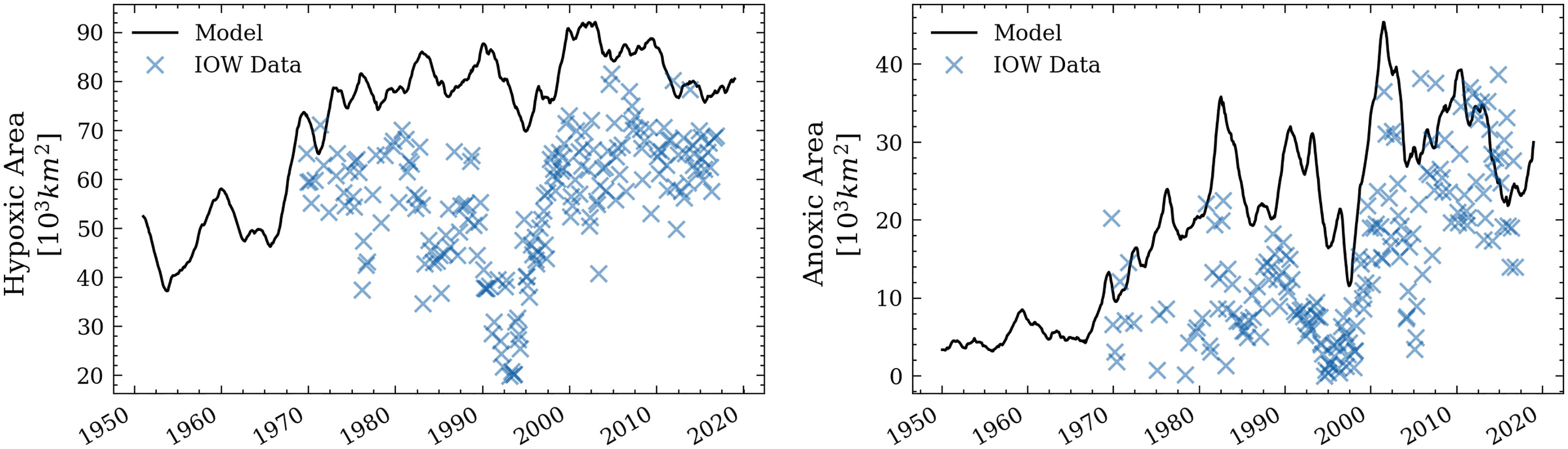
Figure 7 Hypoxic and anoxic area in the Baltic Sea. IOW data taken from Feistel et al. (2016). For better comparison, the analysis follows the domain considered in Krapf et al. (2022) (see Figure 1, grey rectangle).

Altogether, we conclude that the model system is suitable for this study.

3 Results

3.1 Reference simulation

The reference simulation covers the period 950 to 1800, starting with the beginning of the MCA and transitioning around 1350 to the LIA. The average salinity of the Baltic Sea during that period is 6.85 g/kg. In our simulation, the MCA is characterized by higher precipitation and strong westerlies, increased river runoff, and consequently hampered transport of highly saline water from the North Sea (Stigebrandt, 1983; Rodhe and Winsor, 2002; Meier and Kauker, 2003). Hence, the mean salinity of the Baltic Sea decreases by about 0.6 g/kg during the MCA (see Figure 8). After the transition to the LIA, the salinity increases by 0.6 g/kg compared to the mean salinity caused by drier conditions and weaker westerlies. Both periods are subject to strong multidecadal variability.

FIGURE 8

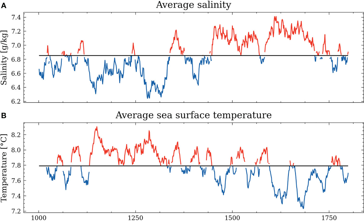
Figure 8 Volume averaged salinity anomaly of the Baltic Sea (A) and volume averaged sea surface temperature anomaly of the Baltic Sea (B). The red (blue) coloring indicates positive (negative) anomalies.

The sea surface temperature also experiences a transition between the MCA and the LIA. The onset of the MCA is still subject to strong multidecadal variability, but after 1050, we find positive temperature anomalies of about 0.5°C compared to the mean SST. Around 1300 to 1400, temperature anomalies start to decrease, reaching their minimum at around 1700 with temperatures -0.6°C colder than average (Figure 8). Following the observed temperature anomaly and considering the spin-up time of the model, we define the MCA from 1050 to 1300 and the LIA from 1400 to 1700.

Not only do the physical parameters experience a shift between the MCA and the LIA, but also the biogeochemical parameters. We use segmented linear regression (Pilgrim, 2021) with one breakpoint on the 10-year low pass-filtered time series to analyze the shifts. The resulting breakpoints (Muggeo, 2003) help quantify an abrupt change in the response function. The results show that in all parameters except for the phosphate in sediment, breakpoints are estimated at the end of the MCA, indicating a regime shift between the MCA and the LIA. For phosphate in sediment, the algorithm did not converge, indicating that no systematic regime shift can be found. During the MCA, the water-column phosphate concentrations, plankton abundance, and nitrogen fixation rates all increase. Conversely, these parameters decrease during the transition to the LIA after 1300 C.E. The phosphorus stored in sediment follows a similar trend but with an estimated breakpoint at 1500 C.E. Lastly, the hypoxic area and the anoxic area strongly increase during the MCA and decrease during the LIA with estimated breakpoints at the end of the MCA (Figure 9).

FIGURE 9

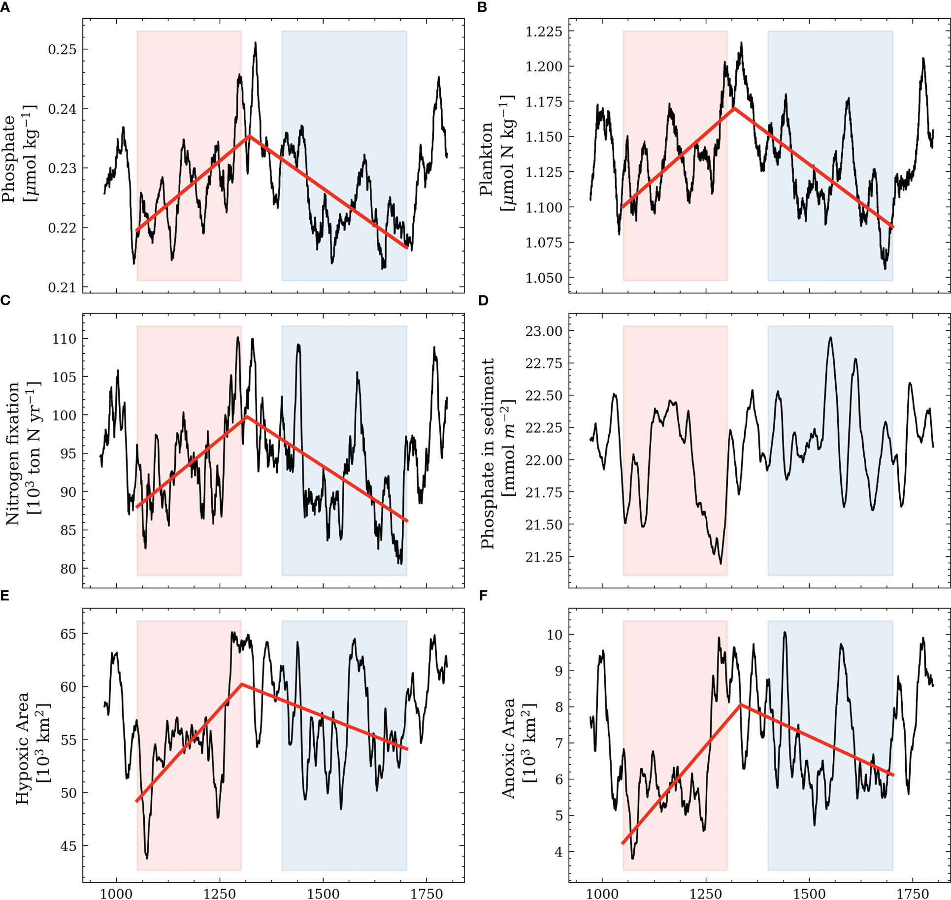
Figure 9 Average biogeochemical parameters in the model with a 10-year running mean. (A) shows winter surface phosphate (December, January, February). (B) shows plankton during summer in nitrogen units (March-September). (C) shows the annual nitrogen fixation. (D) shows phosphate in the sediment. (E) shows the hypoxic area. (F) shows the anoxic area. The domain for the analysis follows Krapf et al. (2022). The red and blue coloring corresponds to the MCA and the LIA, respectively. The red line shows the segmented linear regression using two segments.

While the observed long-term trends for the biogeochemical parameters indicate different regimes between the MCA and the LIA, the parameters also show variability on shorter time scales. For example, the water-column phosphate levels show distinct peaks at the end of the MCA (around 1300 C.E.), at 1600 C.E., and 1780 C.E., which are likely linked to the release of iron-bound phosphate from the sediment due to oxygen depletion. In agreement, we find increasing nitrogen fixation and decreasing phosphorus levels in the sediment, and hypoxic and anoxic areas increase during these peaks (Figure 9).

Nevertheless, the results of the reference simulation indicate that there is a regime shift between the MCA and the LIA. To isolate the role of the temperature response between the MCA and the LIA, we conducted three sensitivity experiments, with increased temperatures during the MCA and lower temperatures during the LIA (Figure 10). We find that in all three sensitivity experiments, the hypoxic area and the anoxic area (not shown) proportionally increase to the applied temperature difference (see Figure 10).

FIGURE 10

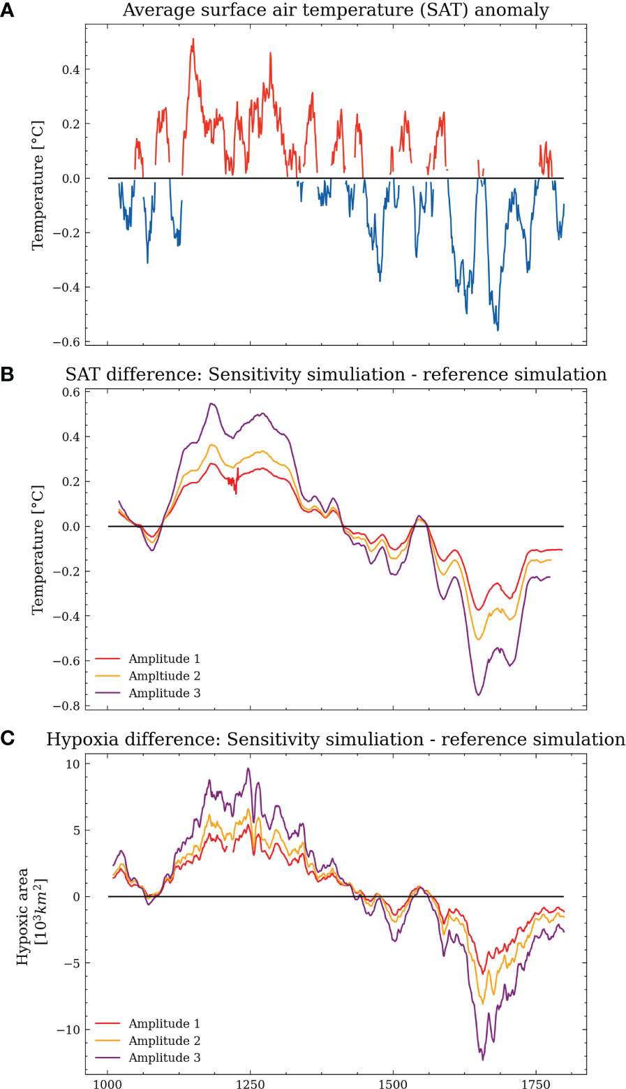
Figure 10 Average surface temperature anomalies of the reference simulation (A, 20-year rolling mean applied). The red (blue) coloring indicates anomalous warm (cold) states. The difference in surface air temperature between Amplitude 1, 2, 3, and the reference simulation (B; 20-year running mean applied), the difference in hypoxic area between Amplitude 1, 2, 3, and the reference simulation (C; 20-year running mean applied).

To address the possible drivers of the increasing (decreasing) hypoxia during the MCA (LIA), we compare the difference in the biogeochemical variables in the water column. As the temperature signal is the strongest in Amplitude 3, the following analysis will compare the difference between Amplitude 3 and the reference simulation (Figure 11).

FIGURE 11

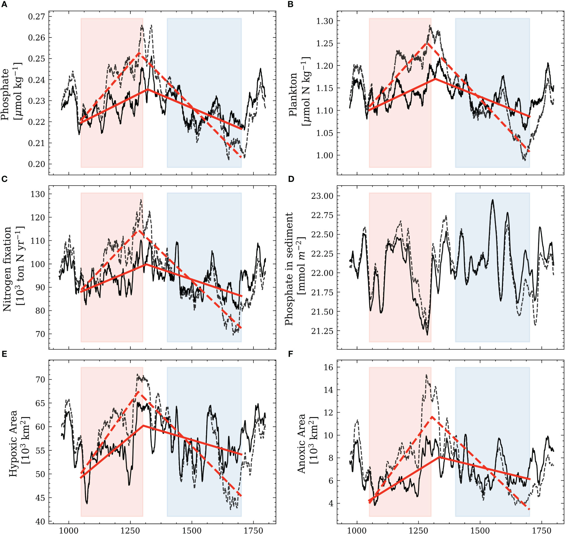
Figure 11 Same as in Figure 9. The solid lines correspond to the reference simulation and reflect the results of Figure 9. The dashed lines show the results of the Amplitude 3 simulation.

The phosphate concentration, plankton concentration, nitrogen fixation, and available phosphate in the sediment increase during the MCA and decrease during the LIA in Amplitude 3 compared to the reference simulation. This suggests a possible coupling between temperature changes and primary production. Under warmer conditions during the MCA in ‘Amplitude 3’, the hypoxic and anoxic areas show a stronger increase. The decrease in hypoxic and anoxic areas is more pronounced during the colder climate in the LIA in ‘Amplitude 3’. In addition, we notice that the location of the estimated breakpoints remains relatively constant compared to the reference simulation.

While the increase in primary production likely drives the hypoxia response during a warmer climate, the oxygen solubility also decreases, possibly leading to lower oxygen levels. To exclude the effect of oxygen solubility, we calculate the apparent oxygen utilization (AOU), here shown for the Gotland Deep Station (Figure 12). The AOU is a measure of oxygen consumption. We find that during the MCA, the oxygen consumption below the permanent halocline increases, which agrees with the higher phytoplankton abundance found in Figure 11. During the LIA, the lower AOU is also confirmed by the decreasing primary production.

FIGURE 12

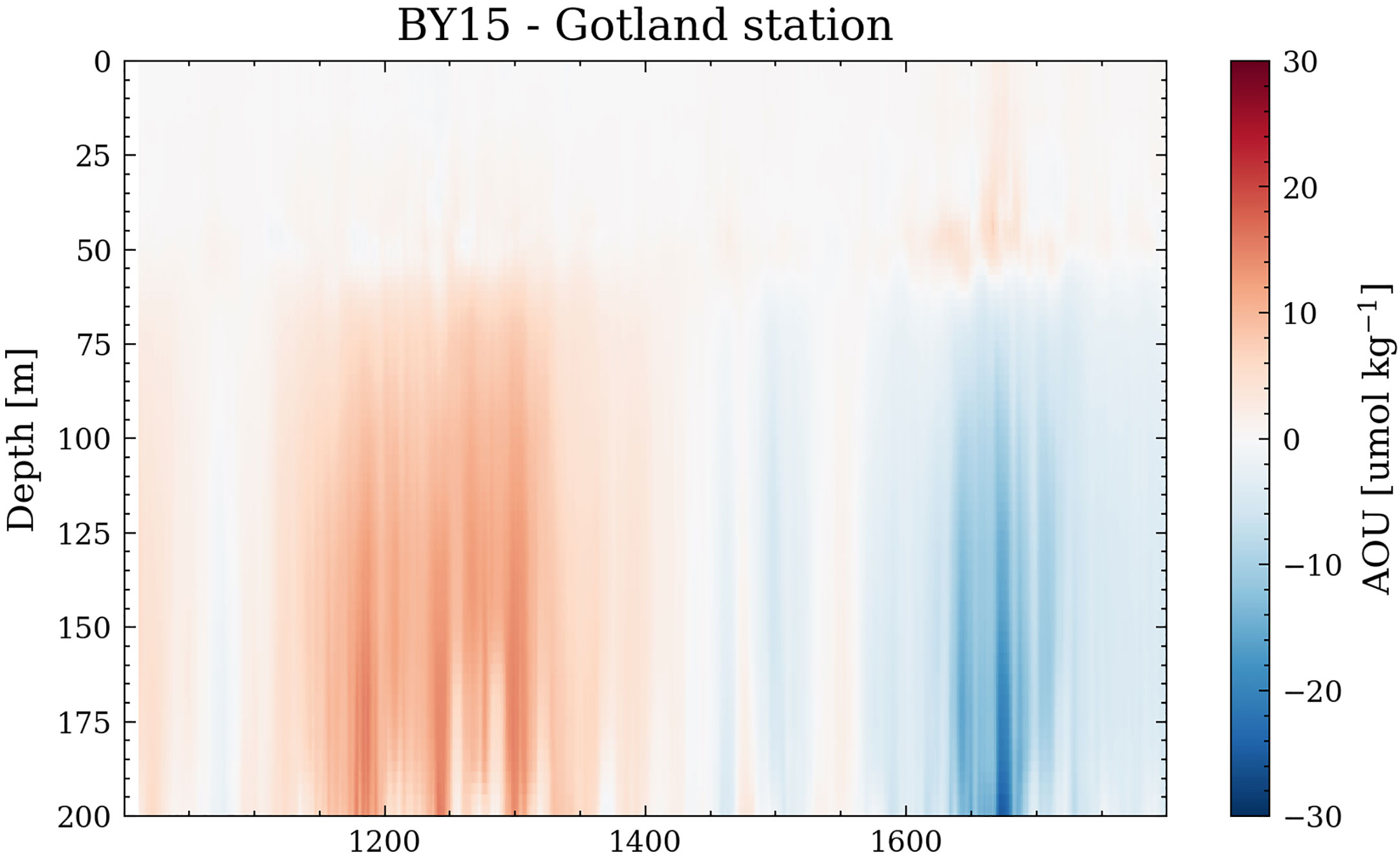
Figure 12 Apparent oxygen utilization at Gotland Station. The yearly difference between the Amplitude 3 simulation and the reference simulation is displayed.

Increased phosphate concentrations and the increase in nitrogen fixation in Amplitude 3 during the MCA (Figures 11A, B) could be related to stronger cyanobacteria blooms that ultimately trigger the positive feedback mechanism when hypoxia is formed (Warden et al., 2017). To test the role of increased cyanobacteria blooms, we calculate the lead-lag correlation between the hypoxic area and cyanobacteria blooms (not shown). We apply a 10-year running mean for the lead-lag analysis, as both variables are strongly coupled on decadal time scales (Andrén et al., 2020). For both model simulations, the cyanobacteria blooms lead the hypoxic area by roughly eight years. However, there is a stronger correlation in Amplitude 3 (0.78), suggesting that cyanobacteria blooms have a larger effect on the hypoxic area than in the reference run (0.52).

While an increased role of cyanobacteria blooms during a warmer climate is likely, we also observe increased primary production for all plankton, despite constant nutrient input. With a changing climate, the mineralization rate also changes, possibly leading to a faster availability of previously consumed nitrogen and phosphorus (Kuliński et al., 2022). Further, preferential mineralization of P is enhanced under anoxic conditions (Jilbert et al., 2011). Therefore, we cannot conclude from our model experiments a mechanistic cause-effect chain explaining the temperature effect on oxygen concentrations on a process level.

For this reason, we perform two additional sensitivity studies. In the first one (Mineral), we artificially increase the water temperature that is used for the mineralization rate in the sediment by 20%. The real water temperature remains unchanged, allowing us to isolate the role of the mineralization rate. In the experiment CYA, we repeat the same procedure for the temperature that the cyanobacteria feel. We increase the temperature (in °C) by 7.5%, roughly resulting in the same temperature change as for the mineralization rate at the bottom (Figure 13).

FIGURE 13

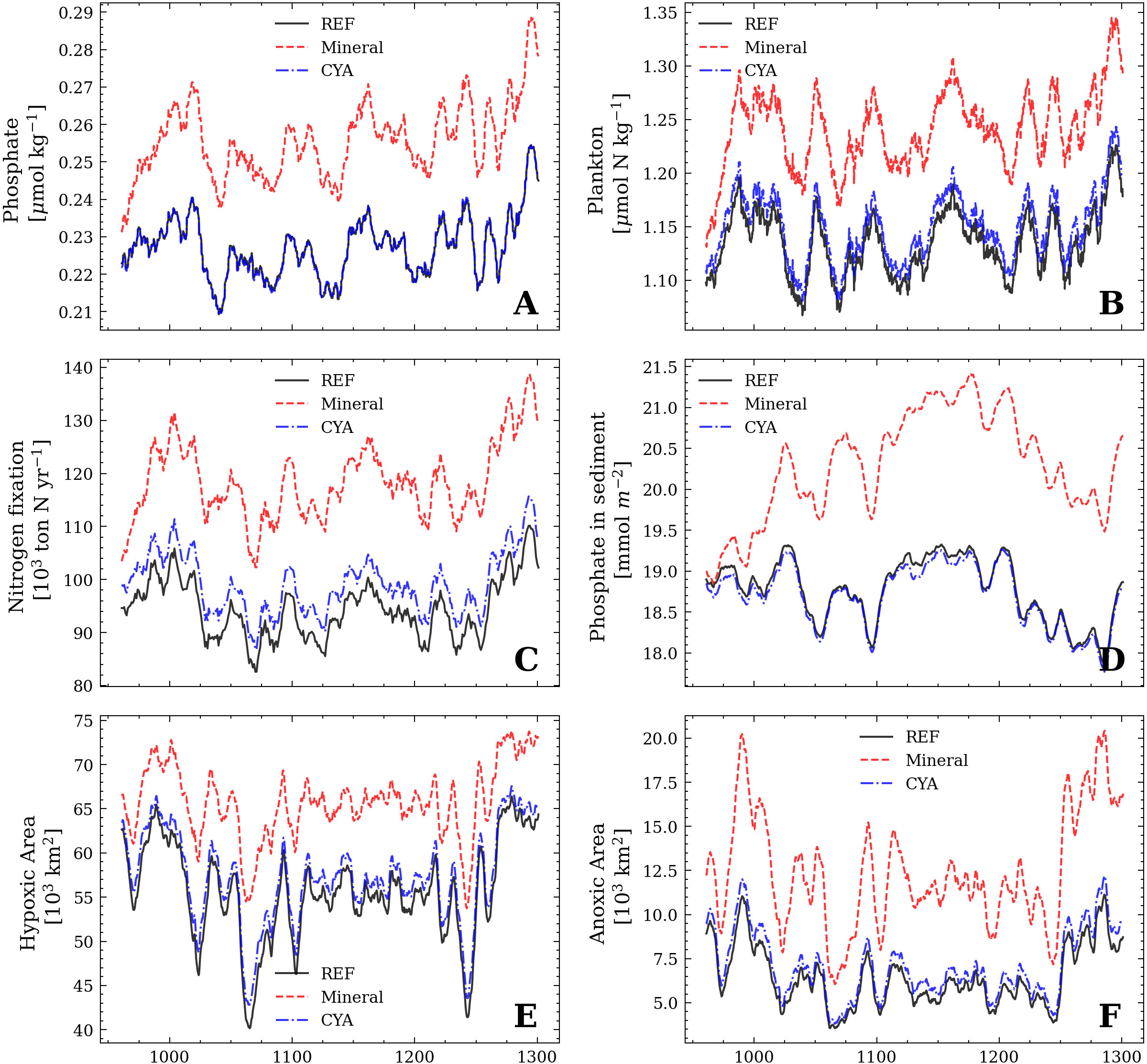
Figure 13 Same as in Figure 9. The solid lines correspond to the reference simulation and reflect the results of Figure 9. The dashed lines (red and blue) show the results of the Mineral and the CYA experiment.

We find that increasing the temperature of the mineralization rate in the sediment has a strong effect on all biogeochemical processes. Compared to the reference simulation, phosphate levels, primary production, and hypoxic and anoxic areas are increased. In contrast, increasing the temperature sensitivity of the cyanobacteria growth rate does not result in any significant changes compared to the reference simulation.

Lastly, we compute the difference in the permanent phosphorus burial between the reference simulation and the Mineral simulation (Figure 14). The results show higher permanent phosphorus burial for the reference simulation in the first 100 years. After 100 years, the system appears to reach an equilibrium with slightly higher permanent phosphorus burial in the reference simulation.

FIGURE 14

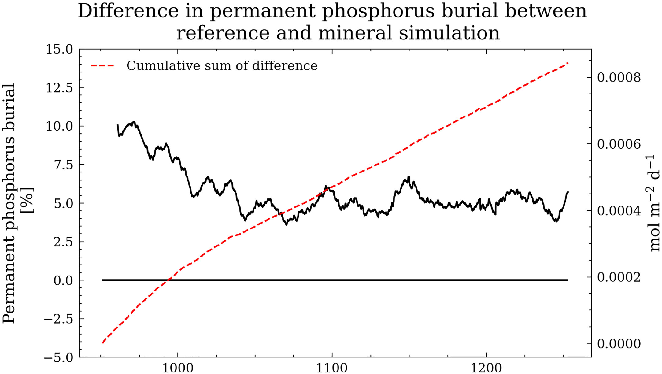
Figure 14 The difference in permanent phosphorus burial between the reference simulation and the Mineral simulation in black (10-year running mean applied). The red dashed curve shows the cumulative sum of the difference.

4 Discussion

Our coupled physical-biogeochemical model showed a clear reaction to temperature changes between MCA and LIA. Increasing the temperature difference between the MCA and the LIA within the uncertainty of proxy data (Kabel et al., 2012; Schimanke et al., 2012) increased hypoxia during the MCA and lowered hypoxia during the LIA. Low nutrient concentrations during the pre-industrial times limit plankton growth. Hence, increasing hypoxia during the MCA has been attributed to stronger nitrogen-fixing cyanobacteria blooms that triggered a positive feedback mechanism (Kabel et al., 2012; Warden et al., 2017; Kahru et al., 2020). Unlike previously assumed, our sensitivity studies indicate that temperature-induced cyanobacteria blooms in a warmer climate are not driving hypoxia. Instead, an enhanced sediment mineralization rate during the warmer MCA increases the primary production by strengthening the biological carbon pump.

Our model also simulates higher cyanobacteria concentrations under a warmer climate. However, they appear not to be triggered by higher surface temperatures, as a higher temperature sensitivity for cyanobacterial growth did not affect the overall hypoxia (sensitivity experiment CYA). In contrast, higher bottom-water temperatures increased sedimentary mineralization rates and the recycling of phosphate to the water column, thereby providing the critical nutrients for cyanobacteria to grow. Kullenberg (1970) estimated a 7% oxygen consumption increase per degree warming, supporting these findings. The experiment “Mineral” shows that the sensitivity of sedimentary mineralization to the bottom-water temperature has a large impact on the model-predicted extent of hypoxia.

Like other biogeochemical models [e.g. IPSL-PISCES (Aumont et al., 2015)] ERGOM uses a temperature sensitivity coefficient ($Q_{10}$) for mineralization. Laufkötter et al. (2017) argue that the temperature dependence of mineralization rate remains a critical difference in model parametrizations, influencing oxygen minimum zones and, thereby, the response of the carbon cycle to warming. The temperature effect on pelagic mineralization has also been inferred from paleoclimate studies, leading to faster recycling of nutrients (John et al., 2014). Based on field data, Q₁₀ values between 1.5 and 2.0 have been estimated for mineralization in ocean water (Laufkötter et al., 2017), which implies a ~ 20% increase in mineralization rates per Kelvin, leading to increasing eutrophication in a warming climate. Estimated $Q_{10}$ values for benthic mineralization have been similar to those for pelagic mineralization (Thamdrup et al., 1998). A similar temperature-dependence for organisms living in sediments or open water can be expected based on theoretical considerations (Arrhenius, 1908; Brown et al., 2004). Yet, it has been observed that benthic metabolism in colder environments is not necessarily lower than in warmer regions (Arnosti et al., 1998). In incubation experiments wherein the temperature is manipulated, microbial communities in sediments are able to adapt to changes in temperature and thereby weaken the temperature-dependence of metabolic rates (Thamdrup et al., 1998; Finke and Jørgensen, 2008; Scholze et al., 2021). Hence, extrapolating $Q_{10}$ values in long-term climate studies may be misleading (Jørgensen, 2021). However, since the 1960s higher residual bottom-water temperatures in the Baltic Sea have been linked to oxygen depletion, possibly caused by increased mineralization, as discussed by Krapf et al. (2022). Lastly, most mineralization in the Baltic Sea appears to take place in sediments, supporting the temperature sensitivity of benthic mineralization as it is implemented in the ERGOM model.

We find that (1) faster mineralization enhances the vertical phosphorus (P) flux leading to (2) higher primary production. (3) For a short time, we observe lower permanent burial, which will, however, return to previous levels since it is compensated by (4) higher detritus sedimentation. This chain of effects is supported by a conceptual 0-dimensional model, isolating these sediment dynamics (see Supplementary Material). This 0-d model suggests that after a temperature increase and assuming constant nutrient loads, the ecosystem will evolve into an altered steady state with higher rates of all biogeochemical processes, except for the burial of phosphorus, which in a steady state, needs to be equal to the P input. The P budget in our 3-d simulation shows that the mechanism is the same. However, due to its connection with the North Sea, higher phosphorus levels in the Baltic Sea will also lead to more phosphorus outflow. Therefore, in our Mineral experiment, the permanent burial never returns precisely to the previous values but shows a deviation within a 5% range after an initial period of approximately 100 years (Figure 14).

Lastly, it should be noted that implementing the sediment model also constrains our results since a maximum sedimentary carbon level is defined, after which permanent burial takes place. Further, stronger westerlies and increased river runoff, as predicted by the atmospheric forcing used in this study, a characteristic of positive NAO phases, can lead to the dilution of surface water, restrained saltwater inflow from the North Sea, and enhanced vertical mixing, which would have counteracted the formation of hypoxia during the MCA (Zorita and Laine, 2000; Schimanke et al., 2012). These atmospheric conditions (of stronger westerlies) are challenged by recent proxy data suggesting a salinity increase in the Baltic Sea during the MCA (Andrén et al., 2020). Hence, the effect of higher temperatures during MCA on hypoxia could have been even larger but was likely masked by the previously discussed processes.

The self-eutrophication linked to temperature-accelerated sediment mineralization should be most prominent in shallow seas. Here, a strong coupling between the ocean floor and the euphotic zone exists. Thus, mineralized nutrients are available for primary production within a short time. In the deep ocean, this mechanism likely plays a less important role, as mineralization in the water column is most important for nutrient recycling. While mineralization in the water column is also temperature-dependent, recycled nutrients are distributed over a large depth range, making location and physical settings in the upper water more important.

Our results introduce enhanced sediment mineralization as a primary driver of hypoxia during the MCA, thus questioning the hypothesis that increased cyanobacteria blooms are the reason for increased hypoxia in the Baltic Sea during the MCA. Further, we argue that future research should revisit the role of the temperature-dependent mineralization in current projections (Meier et al., 2019a; Meier et al., 2019b; Saraiva et al., 2019) as nutrient reductions scenarios for the Baltic Sea such as the Baltic Sea Action Plan (BSAP) could be significantly counteracted by climate change, specifically due to enhanced bottom temperatures, which needs to be considered in future research.

Data availability statement

The raw data supporting the conclusions of this article will be made available by the authors, without undue reservation.

Author contributions

FB designed the research with the help of TN. Both analyzed the model results. FB wrote the manuscript with the help of all co-authors who all contributed to the scientific results presented in this work. FB performed the model simulation, while TN prepared the experiments Mineral and CYA presented in this work. All authors contributed to the article and approved the submitted version.

Acknowledgments

We thank two reviewers who greatly improved earlier versions of this manuscript. The research presented in this study is part of the Baltic Earth program (Earth System Science for the Baltic Sea region, see www.baltic.earth).

Conflict of interest

The authors declare that the research was conducted in the absence of any commercial or financial relationships that could be construed as a potential conflict of interest.

Publisher’s note

All claims expressed in this article are solely those of the authors and do not necessarily represent those of their affiliated organizations, or those of the publisher, the editors and the reviewers. Any product that may be evaluated in this article, or claim that may be made by its manufacturer, is not guaranteed or endorsed by the publisher.

Supplementary material

The Supplementary Material for this article can be found online at: https://www.frontiersin.org/articles/10.3389/fmars.2023.1174039/full#supplementary-material

References

Almroth-Rosell E., Eilola K., Hordoir R., Meier H. E. M., Hall P. O. J. (2011). Transport of fresh and resuspended particulate organic material in the Baltic Sea [[/amp]]mdash; a model study. J. Mar. Syst. 87, 1–12. doi: 10.1016/j.jmarsys.2011.02.005

CrossRef Full Text | Google Scholar

Andrén E., van Wirdum F., Norbäck Ivarsson L., Lonn M., Moros M., Andren T. (2020). Medieval versus recent environmental conditions in the Baltic proper, what was different a thousand years ago? Palaeogeogr. Palaeoclimatol. Palaeoecol. 555, 109878. doi: 10.1016/j.palaeo.2020.109878

CrossRef Full Text | Google Scholar

Arnosti C., Jørgensen B. B., Sagemann J., Thamdrup B. (1998). Temperature dependence of microbial degradation of organic matter in marine sediments: polysaccharide hydrolysis, oxygen consumption, and sulfate reduction. Mar. Ecol. Prog. Ser. 165, 59–70. doi: 10.3354/meps165059

CrossRef Full Text | Google Scholar

Arrhenius S. (1908). Immunochemie. Ergebnisse der Physiologie 7, 480–551. doi: 10.1007/BF02321079

CrossRef Full Text | Google Scholar

Aumont O., Ethé C., Tagliabue A., Bopp L., Gehlen M. (2015). Pisces-v2: an ocean biogeochemical model for carbon and ecosystem studies. Geoscientific Model. Dev. 8, 2465–2513. doi: 10.5194/gmd-8-2465-2015

CrossRef Full Text | Google Scholar

Berliand M. E., Berliand T. G. (1952). Measurement of the effective radiation of the earth with varying cloud amounts. Russian Izv. Akad. Nauk. SSSR 1, 64–78.

Google Scholar

Bodin S. (1979). A predictive numerical model of the atmospheric boundary layer based on the turbulent energy equation. SMHI Rapporter. Meteorologi och Klimatologi RMK 13, 138.

Google Scholar

Breitburg D., Levin L. A., Oschlies A., Grégoire M., Chavez F. P., Conley D. J., et al. (2018). Declining oxygen in the global ocean and coastal waters. Sci. (New York N.Y.) 359. doi: 10.1126/science.aam7240

CrossRef Full Text | Google Scholar

Brown J. H., Gillooly J. F., Allen A. P., Savage V. M., West G. B. (2004). Toward a metabolic theory of ecology. Ecology 85, 1771–1789. doi: 10.1890/03-9000

CrossRef Full Text | Google Scholar

Burchard H., Rennau H. (2008). Comparative quantification of physically and numerically induced mixing in ocean models. Ocean Model. 20, 293–311. doi: 10.1016/j.ocemod.2007.10.003

CrossRef Full Text | Google Scholar

Conley D. J., Björk S., Bonsdorff E., Carstensen J., Destouni G., Gustafsson B. G., et al. (2009). Hypoxia-related processes in the Baltic Sea. Environ. Sci. Technol. 43, 3412–3420. doi: 10.1021/es802762a.414

PubMed Abstract | CrossRef Full Text | Google Scholar

Conley D. J., Humborg C., Rahm L., Savchuk O. P., Wulff F. (2002). Hypoxia in the Baltic Sea and basin-scale changes in phosphorus biogeochemistry. Environ. Sci. Technol. 36, 5315–5320. doi: 10.1021/es025763w

PubMed Abstract | CrossRef Full Text | Google Scholar

Feistel S., Feistel R., Nehring D., Matthaus W., Nausch G., Naumann M. (2016). Hypoxic and anoxic regions in the Baltic Sea, 1969 - 2015. meereswissenschaftliche berichte no 100 2016 - marine science reports no 100 2016, Vol. 138. 85. doi: 10.12754/MSR-2016-0100

CrossRef Full Text | Google Scholar

Fennel K., Testa J. M. (2019). Biogeochemical controls on coastal hypoxia. Annu. Rev. Mar. Sci. 11, 105–130. doi: 10.1146/annurev-marine-010318-095138

CrossRef Full Text | Google Scholar

Finke N., Jørgensen B. B. (2008). Response of fermentation and sulfate reduction to experimental temperature changes in temperate and arctic marine sediments. ISME J. 2, 815–829. doi: 10.1038/ismej.2008.20

PubMed Abstract | CrossRef Full Text | Google Scholar

Funkey C. P., Conley D. J., Reuss N. S., Humborg C., Jilbert T., Slomp C. P. (2014). Hypoxia sustains cyanobacteria blooms in the Baltic Sea. Environ. Sci. Technol. 48, 2598–2602. doi: 10.1021/es404395a

PubMed Abstract | CrossRef Full Text | Google Scholar

Garcia H. E., Boyer T. P., Levitus S., Locarnini R. A., Antonov J. (2005). On the variability of dissolved oxygen and apparent oxygen utilization content for the upper world ocean: 1955 to 1998. Geophys. Res. Lett. 32. doi: 10.1029/2004GL022286

CrossRef Full Text | Google Scholar

Geyer B. (2014). High-resolution atmospheric reconstruction for Europe 1948-2012: CoastDat2. Earth System Sci. Data 6, 147–164. doi: 10.5194/essd-6-147-2014

CrossRef Full Text | Google Scholar

Geyer B., Rockel B. (2013). Coastdat-2 cosmo-clm atmospheric reconstruction. doi: 10.1594/WDCC/coastDat-2\COSMO-CLM

PubMed Abstract | CrossRef Full Text | Google Scholar

Giesse C., Meier H. E. M., Neumann T., Moros M. (2020). Revisiting the role of convective deep water formation in northern Baltic Sea bottom water renewal. J. Geophys. Res.: Oceans 125. doi: 10.1029/2020JC016114

CrossRef Full Text | Google Scholar

Griffies S. M. (2004). Fundamentals of ocean climate models (Princeton University Press).

Google Scholar

Gustafsson B. G., Schenk F., Blenckner T., Eilola K., Meier H. E. M., Muller-Karulis B., et al. (2012). Reconstructing the development of Baltic Sea eutrophication 1850–2006. Ambio 41, 534–548. doi: 10.1007/s13280-012-0317-y

PubMed Abstract | CrossRef Full Text | Google Scholar

Hansson D., Gustafsson E. (2011). Salinity and hypoxia in the Baltic Sea since A.D. 1500. J. Geophys. Res.: Oceans 116. doi: 10.1029/2010JC006676

CrossRef Full Text | Google Scholar

HELCOM (2018). Sources and pathways of nutrients to the Baltic Sea (plc-6). Balt. Sea Environ. Proc. 153.

Google Scholar

Hünicke B., Zorita E., Haeseler S. (2010). GKSS 2010/2 Baltic Holocene climate and regional Sea-level change: a statistical analysis of observations, reconstructions and simulations within present and past as analogues for future changes.

Google Scholar

Hunke E. C., Dukowicz J. K. (1997). An elastic-viscous-plastic model for sea ice dynamics. J. Phys. Oceanogr. 27, 1849–1867. doi: 10.1175/1520-0485(1997)027h1849:AEVPMFi2.0.CO;2

CrossRef Full Text | Google Scholar

Ingall E. D., Bustin R. M., Van Cappellen P. (1993). Influence of water column anoxia on the burial and preservation of carbon and phosphorus in marine shales. Geochimica Cosmochimica Acta 57, 303–316. doi: 10.1016/0016-7037(93)90433-W

CrossRef Full Text | Google Scholar

Jilbert T., Slomp C. P., Gustafsson B. G., Boer W. (2011). Beyond the fe-p-redox connection: preferential regeneration of phosphorus from organic matter as a key control on Baltic Sea nutrient cycles. Biogeosciences 8, 1699–1720. doi: 10.5194/bg-8-1699-2011

CrossRef Full Text | Google Scholar

John E. H., Wilson J. D., Pearson P. N., Ridgwell A. (2014). Temperature-dependent remineralization and carbon cycling in the warm eocene oceans. Palaeogeogr. Palaeoclimatol. Palaeoecol. 413, 158–166. doi: 10.1016/j.palaeo.2014.05.019

CrossRef Full Text | Google Scholar

Jokinen S. A., Virtasalo J. J., Jilbert T., Kaiser J., Dellwig O., Arz H. W., et al. (2018). A 1500-year multiproxy record of coastal hypoxia from the northern Baltic Sea indicates unprecedented deoxygenation over the 20th century. Biogeosciences 15, 3975–4001. doi: 10.5194/bg-15-3975-2018

CrossRef Full Text | Google Scholar

Jørgensen B. B. (2021). Sulfur biogeochemical cycle of marine sediments. Geochem. Perspect. 10, 145–146. doi: 10.7185/geochempersp.10.2

CrossRef Full Text | Google Scholar

Kabel K., Moros M., Porsche C., Neumann T., Adolphi F., Andersen T. J., et al. (2012). Impact of climate change on the Baltic Sea ecosystem over the past 1,000 years. Nat. Climate Change 2, 871–874. doi: 10.1038/nclimate1595

CrossRef Full Text | Google Scholar

Kahru M., Elmgren R., Kaiser J., Wasmund N., Savchuk O. (2020). Cyanobacterial blooms in the Baltic Sea: correlations with environmental factors. Harmful Algae 92, 101739. doi: 10.1016/j.hal.2019

PubMed Abstract | CrossRef Full Text | Google Scholar

Krapf K., Naumann M., Dutheil C., Meier H. E. M. (2022). Investigating hypoxic and euxinic area changes based on various datasets from the Baltic Sea. Front. Mar. Sci. 9. doi: 10.3389/fmars.2022.823476

PubMed Abstract | CrossRef Full Text | Google Scholar

Kuliński K., Rehder G., Asmala E., Bartosova A., Carstensen J., Gustafsson B., et al. (2022). Biogeochemical functioning of the Baltic Sea. Earth System Dynam. 13, 633–685. doi: 10.5194/esd-13-633-2022

CrossRef Full Text | Google Scholar

Kullenberg G. (1970). On the oxygen deficit in the Baltic deep water. Tellus 22, 357–357. doi: 10.1111/j.2153-3490.1970.tb00502.x

CrossRef Full Text | Google Scholar

Laufkötter C., John J. G., Stock C. A., Dunne J. P. (2017). Temperature and oxygen dependence of the remineralization of organic matter: REMINERALIZATION OF ORGANIC MATTER. Global Biogeochem. Cycles 31, 1038–1050. doi: 10.1002/2017GB005643

CrossRef Full Text | Google Scholar

Mann M. E., Zhang Z., Rutherford S., Bradley R. S., Hughes M. K., Shindell D., et al. (2009). Global signatures and dynamical origins of the little ice age and medieval climate anomaly. Science 326, 1256–1260. doi: 10.1126/science.1177303

PubMed Abstract | CrossRef Full Text | Google Scholar

Meier H. E. M., Doscher R., Doos K. (1999). RCO - rossby centre regional ocean climate model: model description (version 1.0) and first results from the hindcast period 1992/93. SMHI. SMHI Rep. Oceanogr. 26, 91–98.

Google Scholar

Meier H. E. M., Edman M., Eilola K., Placke M., Neumann T., Andersson H. C., et al. (2019a). Assessment of uncertainties in scenario simulations of biogeochemical cycles in the Baltic Sea. Front. Mar. Sci. 6. doi: 10.3389/fmars.2019.00046.399

CrossRef Full Text | Google Scholar

Meier H. E. M., Eilola K., Almroth-Rosell E., Schimanke S., Kniebusch M., Hoglund A., et al. (2019b). Disentangling the impact of nutrient load and climate changes on Baltic Sea hypoxia and eutrophication since 1850. Climate Dynam. 53, 1145–1166. doi: 10.1007/s00382-018-4296-y

CrossRef Full Text | Google Scholar

Meier H. E. M., Kauker F. (2003). Modeling decadal variability of the Baltic Sea: 2. role of freshwater inflow and Large-scale atmospheric circulation for salinity. J. Geophys. Res.: Oceans 108, 3368. doi: 10.1029/2003JC001799

CrossRef Full Text | Google Scholar

Meier H. E. M., Vali G., Naumann M., Eilola K., Frauen C. (2018). Recently accelerated oxygen consumption rates amplify deoxygenation in the baltic sea. J. Geophys. Res.: Oceans 123, 3227–3240. doi: 10.1029/2017JC013686

CrossRef Full Text | Google Scholar

Moros M., Kotilainen A. T., Snowball I., Neumann T., Perner K., Meier H. M., et al. (2020). Is ‘deep-water formation’ in the baltic sea a key to understanding seabed dynamics and ventilation changes over the past 7,000 years? Quaternary Int. 550, 55–65. doi: 10.1016/j.quaint.2020.03.031

CrossRef Full Text | Google Scholar

Mortimer C. H. (1942). The exchange of dissolved substances between mud and water in lakes. J. Ecol. 30, 147–201. doi: 10.2307/2256691

CrossRef Full Text | Google Scholar

Muggeo V. M. R. (2003). Estimating regression models with unknown break-points. Stat Med. 22, 3055–3071. doi: 10.1002/sim.1545

PubMed Abstract | CrossRef Full Text | Google Scholar

Neumann T., Koponen S., Attila J., Brockmann C., Kallio K., Kervinen M., et al. (2021). Optical model for the Baltic Sea with an explicit CDOM state variable: a case study with model ERGOM (version 1.2). Geoscientific Model. Dev. 14, 5049–5062. doi: 10.5194/gmd-14-5049-2021

CrossRef Full Text | Google Scholar

Neumann T., Radtke H., Cahill B., Schmidt M., Rehder G. (2022). Non-redfieldian carbon model for the Baltic Sea (ERGOM version 1.2) – implementation and budget estimates. Geoscientific Model. Dev. 15, 8473–8540. doi: 10.5194/gmd-15-8473-2022

CrossRef Full Text | Google Scholar

Neumann T., Schernewski G. (2008). Eutrophication in the Baltic Sea and shifts in nitrogen fixation analyzed with a 3D ecosystem model. J. Mar. Syst. 74, 592–602. doi: 10.1016/j.jmarsys.2008.05.003

CrossRef Full Text | Google Scholar

Ning W., Nielsen A., Ivarsson L. N., Jilbert T., Akesson C., Slomp C., et al. (2018). Anthropogenic and climatic impacts on a coastal environment in the Baltic Sea over the last 1000 years. Anthropocene 21, 66–79. doi: 10.1016/j.ancene.2018.02.003

CrossRef Full Text | Google Scholar

Norbäck Ivarsson L., Andren T., Moros M., Andersen T. J., Lönn M., Andren E. (2019). Baltic Sea Coastal eutrophication in a thousand year perspective. Front. Environ. Sci. 7. doi: 10.3389/fenvs.2019.00088

CrossRef Full Text | Google Scholar

Pilgrim C. (2021). Piecewise-regression (aka segmented regression) in Python. J. Open Source Software 6, 3859. doi: 10.21105/joss.03859

CrossRef Full Text | Google Scholar

Placke M., Meier H. E. M., Neumann T. (2021). Sensitivity of the Baltic Sea overturning circulation to long term atmospheric and hydrological changes. J. Geophys. Res.: Oceans 126, e2020JC016079. doi: 10.1029/2020JC016079

CrossRef Full Text | Google Scholar

Radtke H., Neumann T., Voss M., Fennel W. (2012). Modeling pathways of riverine nitrogen and phosphorus in the Baltic Sea: pathways of Baltic riverine n and p. J. Geophys. Res.: Oceans 117, C09024. doi: 10.1029/2012JC008119

CrossRef Full Text | Google Scholar

Rodhe J., Winsor P. (2002). On the influence of the freshwater supply on the Baltic Sea mean salinity. Tellus A: Dynamic Meteorol. Oceanogr. 54, 175–186. doi: 10.3402/tellusa.v54i2.12134

CrossRef Full Text | Google Scholar

Samuelsson P., Jones C. G., Willen U., Ullerstig A., Gollvik S., Hansson U. L. F., et al. (2011). The rossby centre regional climate model RCA3: model description and performance. Tellus Ser. A-dynamic Meteorol. Oceanogr. 63, 4–23. doi: 10.1111/j.1600-0870.2010.00478.x

CrossRef Full Text | Google Scholar

Saraiva S., Markus Meier H. E., Andersson H., Hoglund A., Dieterich C., Groger M., et al. (2019). Baltic Sea Ecosystem response to various nutrient load scenarios in present and future climates. Climate Dynam. 52, 3369–3387. doi: 10.1007/s00382-018-4330-0

CrossRef Full Text | Google Scholar

Savchuk O. P. (2018). Large-Scale nutrient dynamics in the Baltic Sea, 1970–2016. Front. Mar. Sci. 5. doi: 10.3389/fmars.2018.00095

CrossRef Full Text | Google Scholar

Schimanke S., Meier H. E. M. (2016). Decadal-to-centennial variability of salinity in the baltic sea. J. Climate 29, 7173–7188. doi: 10.1175/JCLI-D-15-0443.1

CrossRef Full Text | Google Scholar

Schimanke S., Meier H. E. M., Kjellström E., Strandberg G., Hordoir R. (2012). The climate in the Baltic Sea region during the last millennium simulated with a regional climate model. Climate Past 8, 1419–1433. doi: 10.5194/cp-8-1419-2012

CrossRef Full Text | Google Scholar

Schneider B., Nausch G., Pohl C. (2010). Mineralization of organic matter and nitrogen transformations in the gotland Sea deep water. Mar. Chem. 119, 153–161. doi: 10.1016/j.marchem.2010.02.004

CrossRef Full Text | Google Scholar

Scholze C., Jørgensen B. B., Røy H. (2021). Psychrophilic properties of sulfate-reducing bacteria in arctic marine sediments. Limnol. Oceanogr. 66, S293–S302. doi: 10.1002/lno.11586

CrossRef Full Text | Google Scholar

Stigebrandt A. (1983). A model for the exchange of water and salt between the Baltic and the skagerrak. J. Phys. Oceanogr. 13, 411–427. doi: 10.1175/1520-0485(1983)013h0411

CrossRef Full Text | Google Scholar

Stigebrandt A., Andersson A. (2020). The eutrophication of the Baltic Sea has been boosted and perpetuated by a major internal phosphorus source. Front. Mar. Sci. 7. doi: 10.3389/fmars.2020.572994

CrossRef Full Text | Google Scholar

Thamdrup B., Hansen J. W., Jørgensen B. B. (1998). Temperature dependence of aerobic respiration in a coastal sediment. FEMS Microbiol. Ecol. 25, 189–200. doi: 10.1111/j.1574-6941.1998.tb00472.x

CrossRef Full Text | Google Scholar

Vahtera E., Conley D. J., Gustafsson B. G., Kuosa H., Pitkanen H., Savchuk O. P., et al. (2007). Internal ecosystem feedbacks enhance nitrogen-fixing cyanobacteria blooms and complicate management in the Baltic Sea. AMBIO: A J. Hum. Environ. 36, 186–194. doi: 10.1579/0044-7447(2007)36[186:IEFENC]2.0.CO;2

CrossRef Full Text | Google Scholar

Väli G., Meier H. E. M., Elken J. (2013). Simulated halocline variability in the Baltic Sea and its impact on hypoxia during 1961-2007. J. Geophys. Res.: Oceans 118, 6982–7000. doi: 10.1002/2013JC009192

CrossRef Full Text | Google Scholar

van Helmond N. A. G. M., Lougheed B. C., Vollebregt A., Peterse F., Fontorbe G., Conley D. J., et al. (2020). Recovery from multi-millennial natural coastal hypoxia in the Stockholm archipelago, Baltic Sea, terminated by modern human activity. Limnol. Oceanogr. 65, 3085–3097. doi: 10.1002/lno.11575

PubMed Abstract | CrossRef Full Text | Google Scholar

Warden L., Moros M., Neumann T., Shennan S., Timpson A., Manning K., et al. (2017). Climate induced human demographic and cultural change in northern Europe during the mid-Holocene. Sci. Rep. 7, 1–11. doi: 10.1038/s41598-017-14353-5

PubMed Abstract | CrossRef Full Text | Google Scholar

Wasmund N. (1997). Occurrence of cyanobacterial blooms in the baltic sea in relation to environmental conditions. Internationale Rev. der gesamten Hydrobiologie und Hydrographie 82, 169–184. doi: 10.1002/iroh.19970820205

CrossRef Full Text | Google Scholar

Winton M. (2000). A reformulated three-layer Sea ice model. J. Atmospheric Oceanic Technol. 17, 525–531. doi: 10.1175/1520-0426(2000)017h<0525:ARTLSI>i2.0.CO;2

CrossRef Full Text | Google Scholar

Zillen L., Conley D. J. (2010). Hypoxia and cyanobacteria blooms - are they really natural features of the late Holocene history of the Baltic Sea? Biogeosciences 8, 2567–2580. doi: 10.5194/bg-7-2567-2010

CrossRef Full Text | Google Scholar

Zillén L., Conley D. J., Andrén T., Andren E., Björck S. (2008). Past occurrences of hypoxia in the Baltic Sea and the role of climate variability, environmental change and human impact. Earth-Science Rev. 91, 77–92. doi: 10.1016/j.earscirev.2008.10.001

CrossRef Full Text | Google Scholar

Zorita E., Laine A. (2000). Dependence of salinity and oxygen concentrations in the Baltic Sea on Large-scale atmospheric circulation. Climate Res. 14, 25–41. doi: 10.3354/cr014025

CrossRef Full Text | Google Scholar