Development of a high-resolution marine ecosystem model for predicting the combined impacts of ocean acidification and deoxygenation

1 Introduction

A very active area of research in recent years is the study of climate change as well as its underlying causes and consequences. For oceans and coastal areas, there is great concern for the potential negative effects that may be brought about by rising seawater temperatures and sea level rise on both natural ecosystems and human populations (Intergovernmental Panel on Climate Change (IPCC), 2019). And while the mechanisms related to increasing temperatures and sea level rise are relatively well understood, two other consequences related to anthropogenic CO₂ emissions and rising global temperatures need further elucidation, and these are ocean acidification and deoxygenation (e. g., DePasquale et al., 2015; Gobler and Baumann, 2016; IPCC, 2019; Kwiatkowski et al., 2020).

There has been growing concern regarding ocean acidification since the start of the century, particularly for the negative influence it may have on marine calcifying organisms (e.g., Orr et al., 2005; Doney et al., 2009; Fujii et al., 2023). Rising anthropogenic CO₂ emissions into the atmosphere have led to greater oceanic CO₂ uptake, which in turn affects the overall chemical balance and decreases pH levels. More specifically, primarily through uptake into the ocean from the atmosphere, CO₂ entering the ocean reacts with water (H₂O) in seawater to form a weak acid known as carbonic acid (H₂CO₃). The H₂CO₃ then separates into hydrogen ions (H⁺), bicarbonate ions (HCO₃^-), and carbonate ions (CO₃^2-), releasing H⁺into seawater:

$\begin{array}{ll}{\text{CO}}_2+{\text{H}}_2\text{O }\to {\text{H}}_2{\text{CO}}_3\to {\text{HCO}}_3^{-}+{\text{H}}^{+}& (1)\end{array}$

Increasing amounts of CO₂ absorbed by the ocean causes H⁺ concentrations to increase, leading to a decrease in pH, and naturally alkaline seawater becomes more acidic. Hence this overall phenomenon has been termed ocean acidification (Orr et al., 2005; Gattuso and Hansson, 2011; Bates et al., 2014; Jiang et al., 2019).

Yet despite its recognition as a potential threat, assessing the impacts of ocean acidification on marine organisms remains an ongoing challenge. Responses vary among species and may be affected by various factors such as interspecies interactions, nutritional status, or the potential for acclimation or adaptation (e.g., Kroeker et al., 2013). Further complicating the study of ocean acidification is the challenge of properly assessing site-specific ocean acidification states and possible future trajectories. For example, while ocean acidification is a globally occurring phenomenon, the rates and chemical changes are expected to be most striking in higher latitude areas (e.g., Orr et al., 2005; Cummings et al., 2011). Furthermore, pH changes in coastal areas may be affected by multiple factors, such as nutrient inputs from adjacent watersheds, ecosystem metabolic processes, as well as local ocean dynamics (e.g., Duarte et al., 2013).

On the other hand, the impacts of reduced dissolved oxygen (DO) concentrations on marine organisms have been studied from as early as the 1970s (Vaquer-Sunyer and Duarte, 2008). Depending on the DO concentration, seawater can be classified as hypoxic, suboxic, or anoxic (Fennel and Testa, 2019). Oxygen depleted waters have been associated with many coastal waters in bays and estuaries around the world, where high rates of photosynthetic production and dissolution of organic matter has led to high rates of surface O₂ production and subsequent consumption in subsurface waters and sediments. These can then be further exacerbated by eutrophication due to increasing agricultural runoff and sewage inputs (Keeling et al., 2010). An important case in point for Japan is Tokyo Bay, which experiences both ocean acidification and greatly reduced DO concentrations (e.g., Yamamoto-Kawai et al., 2015, Yamamoto-Kawai et al., 2021).

More recently, the possibility of additive or synergistic negative effects on marine organisms when both low DO and low pH occur together has also been drawing more attention (e.g., Melzner et al., 2013; DePasquale et al., 2015). Important knowledge gaps exist, which need to be addressed through increasingly better-designed multi-stressor experimental and field studies to further investigate marine organism responses, as well as through improved monitoring and predictive capabilities for the marine environment under the combined influence of ocean acidification and reduced DO concentrations (Gobler and Baumann, 2016). It has been contended that to properly study ocean acidification in coastal waters, a regional focus is necessary (Duarte et al., 2013). This can even be taken a step further by considering the importance of not only regional influences but also more local factors to provide a more comprehensive evaluation of ocean acidification and deoxygenation in a particular coastal area.

In this study, we describe the development of a marine ecosystem modeling approach which was used to investigate ocean acidification and deoxygenation in an area along the northeastern coast of Japan. In spite of the area being an important source of local fisheries, ocean observational data is very limited, and the main observational dataset used in this study was obtained from a single monitoring station. While recognizing this limitation and also because of this limitation, we proceeded to develop a high-resolution ecosystem model in order to better characterize the physical conditions as well as carbonate parameter trends in the area. The modeling approach was then evaluated using continuous monitoring data from the single monitoring station, which featured measurements of both physical as well as carbonate parameters, to assess its ability to accurately reproduce present day values and trends.

We then proceeded further by modifying the model setup to run historical and future projections based on selected Representative Concentration Pathway (RCP) scenarios (IPCC, 2019). This was made possible through the availability of future projection model output for a number of RCP scenarios which had been run specifically for Japan’s coasts (Nishikawa et al., 2021). The overall results were then used to discuss possible impacts of future ocean acidification and deoxygenation in the area. It is also hoped that this study can contribute to developing a framework for modeling important coastal sites in Japan, which can go hand in hand with the establishment of more monitoring points as well as the improvement of regional model future projections.

2 Methods

2.1 Study site and monitoring setup

Miyako Bay is located along the northeastern coast of the main island Honshu in Iwate Prefecture, Japan (Figure 1A). The bay is well-known for its seaweed, scallop, oyster, abalone, and sea urchin fisheries (Miyako city website: https://www.city.miyako.iwate.jp/suisan/ikuseikyougikai_gyogyoukeitai.html), which also attract tourists and enhance local tourism activities. It has been a known habitat of the eelgrass Zostera marina, and previous hydrodynamically oriented studies have focused on the damage and recovery of the population from the Great Tohoku Earthquake in March 2011 (e.g., Okada et al., 2014; Murakami et al., 2015). However, there is concern that rising sea temperatures along with the possible ocean acidification and deoxygenation may threaten such ecosystem services (Fujita, 2021; Ono et al., 2023). Two rivers, Hei River and Tsugaruishi River, empty into the bay and are considered to be relatively pristine. In the area just north of Miyako Bay, the Japan Fisheries Research and Education Agency (FRA) maintains a marine station where observations of various parameters, including temperature, salinity, carbonate system parameters, and DO, have been taken using a variety of sensors (Figure 1B).

FIGURE 1

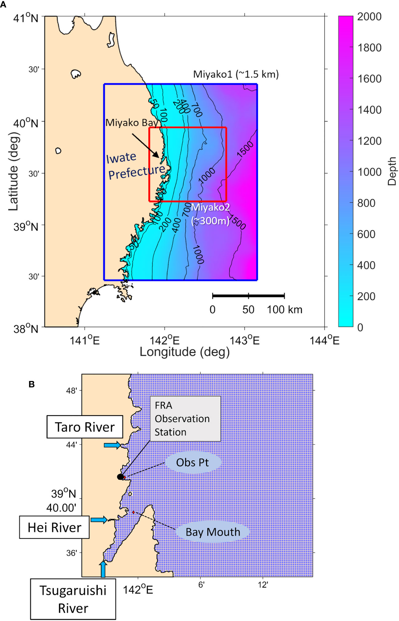
Figure 1 (A) Location of Miyako Bay along the northeastern coast of Honshu, Japan as well as the configuration of the Miyako nested model setup. The 1.5 km grid resolution Miyako1 is initially run and the results are used to generate necessary initial and boundary conditions for the 300 m grid resolution Miyako2. (B) Close-up view of the the 300 m Miyako2 model grid displaying how it resolves the coastal features within and around Miyako Bay. The locations of nearby rivers, FRA monitoring point, and model evaluation points are also shown.

More specifically, a monitoring point was established at approximately 39.69° N Latitude and 141.97° E Longitude. Sensors were not actually deployed at the monitoring point itself, and instead there was an intake at a depth of approximately 5 meters from which seawater was extracted and pumped into storage tanks located at the FRA marine station. The monitoring apparatus was located at the end point of the intake through which seawater flowed on the way to the storage tanks. It consisted of sensors measuring water temperature, salinity, pH (total scale) and DO. The sensor settings and precision information are described in Ono et al. (2023). Sensor measurements taken from July 1, 2020 to September 21, 2021 were used for analysis in this study. Additionally, seawater samples were collected once a week and were analyzed using a total alkalinity (TA) titration analyzer (ATT-05; Kimoto Electric) to obtain the TA and a coulometer (MODEL 3000A; Nippon ANS) to determine the dissolved inorganic carbon (DIC) concentration (Wakita et al., 2017; Yamaka, 2019; Fujii et al., 2021; Wakita et al., 2021). To obtain higher resolution output of TA, an empirical relation for TA and salinity was obtained from water sampling data. Using this relation, TA values at the temporal resolution of the salinity sensor could also be derived. In addition, continuous high-resolution DIC outputs were obtained by using continuous measurements of temperature, salinity, pH as well as the empirically calculated TA outputs in the CO2SYS for Excel program (Lewis et al., 1998; Pierrot et al., 2006) to obtain corresponding DIC values. From October 26, 2021, the monitoring apparatus at the FRA marine station was relocated to a deeper and more offshore location (Omoe) to the east of Miyako Bay, at approximately 39.5947° N Latitude and 142.0458° E Longitude at a deployment depth of 16 meters.

2.2 Model setup

Although limited in space and time, the availability of monitoring data, coupled with the potential for both ocean acidification and deoxygenation to affect local ecosystem services, led us to select the site for performing a high-resolution numerical ecosystem modeling study. A similar modeling system to that described in Fujii et al. (2021) was used, but more features were activated to incorporate important local processes, such as tides, sub-daily meteorological forcing, and inputs from rivers. Future projections have also been enhanced, with initial and boundary forcing generated from recent high-resolution modeling datasets developed specifically for Japanese coastal areas.

The Coastal and Ocean Regional COmmunity (CROCO) modeling system (https://doi.org/10.5281/zenodo.7415055) was selected due to its ability to simulate most of the parameters necessary for our investigation through the coupling of the Regional Ocean Modeling System (ROMS) (Haidvogel et al., 2000; Shchepetkin and McWilliams, 2005) hydrodynamic model and the Pelagic Interactions Scheme for Carbon and Ecosystem Studies (PISCES; Aumont and Bopp, 2006) marine biogeochemical model. And while PISCES has been mainly used to study wide areas and over relatively long periods (e.g. Aumont and Bopp, 2006; Joshi and Warrior, 2022) as well as in earth system models (e.g., Kwiatkowski et al., 2020) we attempt to evaluate its applicability for a much more local area and over a shorter time scale. The CROCO modeling system version 1.1 (Jullien et al., 2019, https://doi.org/10.5281/zenodo.7415055) was used, and as CROCO includes several options for biogeochemical modeling, the PISCES marine biogeochemical model was selected. CROCO was then set up to couple the ROMS and PISCES models and used to reproduce relevant physical and biochemical processes, and make projections of possible future conditions.

A one-way nesting scheme was used, which featured an outer 1.5 km grid resolution coarse domain model (Miyako1) and a nested finer scale 300 m grid resolution model (Miyako2) (Figures 1A, B). Bathymetry for both models was derived from the 15 arc-second GEBCO 2021 dataset (https://www.gebco.net). For the vertical coordinate, 32 and 24 sigma layers were set for Miyako1 and Miyako2, respectively. To simulate present day conditions for comparison with observations, initial and boundary conditions for water temperature, salinity, eastward and northward velocity components, and water surface elevation were derived from the 3-hourly global 1/12° Hybrid Coordinate Modeling System Global Ocean Forecasting System (GOFS) 3.1 Analysis dataset (HYCOM GLBy0.08, https://www.hycom.org/dataserver/gofs-3pt1/analysis). Tidal forcing was also added using components derived from the TPXO7 global tidal solution (Egbert and Erofeeva, 2002, https://www.tpxo.net/global). Meteorological forcing at an hourly interval, which consisted of the parameters air temperature, relative humidity, east-west and south-north wind components, solar radiation, and precipitation, was derived from the Japan Meteorological Agency-Grid Point Value (JMA-GPV) mesoscale model results collected and distributed by the Research Institute for Sustainable Humanosphere, Kyoto University (http://database.rish.kyoto-u.ac.jp/arch/jmadata/gpv-netcdf.html). For the vertical mixing, the generic length scale (GLS) scheme (Umlauf and Burchard, 2003; Warner et al., 2005) was used and the k–ϵ GLS model was selected. Miyako1 was run first, after which initial and boundary conditions were created for Miyako2 based on Miyako1 modeling results. The numerical barotropic timesteps were set as 60 s and 30 s for Miyako1 and Miyako2, respectively.

To run the PISCES biogeochemical model, initial and boundary conditions for Miyako1 were derived from several sources. For silicate (Si), nitrate (NO₃), phosphate (PO₄), and oxygen (O₂), the World Ocean Atlas 2009 (WOA 2009) monthly climatology was used (Garcia et al., 2010a; Garcia et al., 2010b). To provide the best representation for TA and DIC conditions, the empirical relations obtained in Watanabe et al. (2020) for the area off the eastern coast of Japan were used to calculate TA and DIC values from monthly climatological temperature and O₂ derived from the WOA 2009 dataset (Garcia et al., 2010a; Locarnini et al., 2010) (WOA data are available from https://www.ncei.noaa.gov/products/world-ocean-atlas).

Another characteristic of the study site is the presence of river inputs into the coast (Figure 1B). Grid cells within the Miyako2 domain corresponding to river mouths (Hei River, Tsugaruishi River, Taro River) were set up as river inputs in the model. However, as these rivers are relatively small, flow measurement data is limited, and hence monthly averaged flow data for the much larger and well-monitored Kitakami River to the south was used to modify the flow rates using ratios with respect to their known average flow rates (see Supplementary Material Section1, Figure S1; Table TS1). Monthly averaged temperatures in each river were set the same as in Kitakami river, and concentrations for all other PISCES tracers in each river were set as zero or to very low values, except for NO₃ (5.0 µmolN kg^-1), PO₄ (0.3 µmolP kg^-1), Si (65 µmolSi kg^-1), TA and DIC (410 µmol kg^-1 for Hei and Tsugaruishi Rivers, and 142 µmol kg^-1 for Taro River), and O₂ (195 µmol kg^-1), which were based on Kobayashi (1961) and sporadic river water sampling.

The model was given a spin-up period of 1 month and the simulation period for analysis was from July 1, 2020 to March 15, 2022. Model output data was at 6-hour intervals, and time-series results were extracted for a grid cell close to the monitoring point near the FRA marine station as well near the mouth of Miyako Bay. Model performance for the present day simulation was evaluated by comparing simulation results with in-situ observations. Observations for water temperature, salinity, TA, DIC, pH, aragonite saturation state (Ω_arag), and DO were available at the FRA monitoring point to evaluate model performance. In particular, the model provided outputs for temperature, salinity, TA, DIC, and DO and these were compared directly with observations. The model did not directly provide outputs for pH and Ω_arag values, and so these were calculated using the CO2SYS for Excel program (Lewis et al., 1998; Pierrot et al., 2006) from modeled temperature, salinity, TA, and DIC, and then compared with observed values.

2.3 Historical and future scenarios

Historical and future scenario cases were also set up, which used initial and boundary conditions derived from Future Ocean Regional Projection (FORP) simulations run using the MRI-CGCM3 climate projection model (Yukimoto et al., 2012; Tsujino et al., 2017; Nishikawa et al., 2021). The FORP-JPN02 data output is at daily intervals and relatively high-resolution data (~2 km) covering the entire Japan is available for some selected periods and RCP scenarios. Initially, three scenarios were prepared, each involving a 1-year simulation over roughly the same period in a given year. These were a historical scenario (May 2000 to April 2001), and future scenarios for the end of the century (May 2099 to April 2100) under both RCP 2.6 and RCP 8.5 conditions. Temperature, salinity, velocity, and water level data from FORP was used to generate initial and boundary conditions for each scenario for Miyako1. Each scenario used the same tidal forcing as the HYCOM-based present day simulation (corresponding to the time period May 2020 to April 2021) as well as the same atmospheric forcing but with a slight modification. To better represent historical and possible future conditions, surface air temperature corrections were applied for each scenario based on estimated differences with present day values (see Supplementary Material Section 2, Figure S2). Boundary conditions used for nutrients, DO, and TA were the same as for the present day simulation as well. However, future projections for DIC were necessary to create appropriate boundary conditions, and hence these were derived from the Model for Interdisciplinary Research on Climate-Earth System Model (MIROC-ESM; Watanabe et al., 2011) run results for near the end of the century under RCP 2.6 and RCP 8.5 conditions. In addition, representative atmospheric CO₂ concentration (pCO_2air) values were set for each scenario case (historical: 340 ppm; RCP 2.6: 420 ppm; RCP 8.5: 900 ppm) (IPCC, 2019).

The end of the century may seem to be still a long way off, leaving ample time to adapt and prevent a worst-case scenario. So additionally, we also attempted to use our approach to run a scenario for the more foreseeable middle of the century (2050s). FORP data was available to run a scenario for the period May 2050 to April 2051 under RCP 8.5 conditions. As in the previous scenario runs, temperature, salinity, velocity, and water level data from FORP were used to generate initial and boundary conditions for Miyako1. Tidal forcing was again the same as the HYCOM-based present day simulation (corresponding to the time period May 2020 to April 2021), and the same atmospheric forcing was used but with surface air temperature correction applied corresponding to the 2050s under RCP8.5. Boundary conditions for nutrients, O₂, and TA were similar to those for the present day simulation as well. However, as MIROC-ESM output was not available to us for the middle of the century scenario, DIC boundary values for the 2050s were calculated from FORP-predicted temperature and salinity and present day TA boundary values while setting a fixed oceanic CO₂ concentration (pCO_2sea) value of 540 ppm within the CO2SYS program for MATLAB (Lewis et al., 1998; van Heuven et al., 2011). The middle of the century RCP 8.5 simulation was then run with pCO_2air was also similarly set as 540 ppm (IPCC, 2019).

It must be noted that the simulation periods for the historical and future scenarios cases were chosen quite arbitrarily, as representing the start of (May 2000 to April 2001), the middle of (May 2050 to April 2051), and the end of (May 2099 to April 2100) the present century. The inability to generate longer simulation datasets was due to limitations in computational resources, data storage, and time for performing the modeling experiments. In particular, running a coupled physical-biogeochemical model at the spatial resolution we selected and for the number of scenario cases we attempted required very careful management of our computational and data storage resources. Hence, interannual variability, which is found in most environmental parameters and is reflected in the results of global circulation model (GCM) projections for the coming decades (e.g. Drenkard et al., 2021), is not taken into account. Nevertheless, to derive some understanding of the interannual variability involved in MRI-CGCM3-based future projections for the study area, two representative points were chosen: one at the study area and another approximately 50 kilometers offshore. Five years of near-surface temperature and salinity data from the FORP simulations used as boundary conditions were then extracted and plotted for the two points (Figure 2; Supplementary Figure S3). The five-year span chosen included the periods which we used for our historical and future scenarios, and these are indicated in both Figure 2 and Figure S3. From these it can be observed that indeed the dataset can show significant interannual variability. For example, the water temperature trends show that the periods selected for both our RCP8.5 middle of the century and RCP8.5 end of century modeling scenarios appear to be characterized by a relatively cool summer and relatively warm winter compared to preceding years (Figure 2). The trends in salinity appear less regular or cyclic, but the RCP8.5 middle of the century scenario period appears to have a particularly low summer salinity while the RCP2.6 end of century scenario appears to be characterized by lower salinities all year round (Figure S3). Hence, we recognize that our scenario simulations of 1 year duration have the limitation of only being able to assess the conditions of the year being simulated, which may or may not be representative of the surrounding years. However, this is indicative of the tradeoff that results from choosing to work at a higher resolution in order to resolve finer scale coastal features.

FIGURE 2

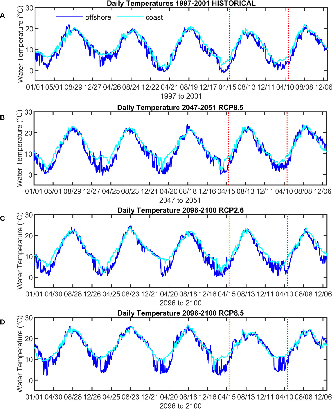
Figure 2 Time series plots of the FORP model output used as initial and boundary conditions for the future projection simulations for a point at the approximate location of the monitoring point (labeled ‘coast’ and represented by cyan colored lines) and another point 50 km offshore to the east (labeled ‘offshore’ and represented by blue colored lines). Five years of simulation results are shown for water temperature at 0.5 m depth with the red dashed lines enclosing the period used to generate boundary conditions for the Miyako model setup for the historical scenario (A), the middle-of-century RCP8.5 scenario (B), the end-of-century RCP2.6 scenario (C), and the end-of-century RCP8.5 scenario (D). Similar plots for salinity can be found in the Supplementary Material (Figure S3).

The interannual variability seen in the FORP model outputs are likely also present in the MIROC-ESM model outputs used as the basis of our DIC initial and boundary conditions for the end of the century RCP2.6 and RCP8.5 scenarios. However, the data was provided to us in the form of monthly climatologies averaging the results from the years 2086-2095, and hence generating time series point data similar to the FORP outputs could not be performed. Nevertheless, as a step towards developing an appropriate modeling approach, we consider that this combination of FORP and MIROC-ESM based initial and boundary conditions at least allows us to simulate plausible conditions for our selected scenario time periods.

3 Results

3.1 Present day simulation

As the study site is located in Japan, dates and times indicated in all figures and tables (including the Supplementary Material) are in Japan Standard Time (JST). Model outputs both from near the FRA marine station observation point as well as from a point located at the mouth of Miyako Bay were extracted and plotted against observations (Figures 1B,  3). Unfortunately, observation data was not available for areas within Miyako Bay, so only observations from near the FRA marine station are shown. In addition, due to some problems in the monitoring apparatus, observations for carbonate parameters and DO were found to be highly inaccurate for a part of the measurement period, and so observations for these parameters from January 1 to May 31, 2021 have been omitted in the plots. The model simulated water temperature and salinity quite accurately (Figures 3A, B), except for some prominent drops in salinity during the summer to autumn season of 2020 and in mid-August to early September 2021. These salinity drawdowns appear to be mirrored in the TA observations for these periods, which the model was also not able to accurately reproduce (Figure 3C). The seasonal changes in DIC however appear to have been mostly reproduced in the model (Figure 3D).

FIGURE 3

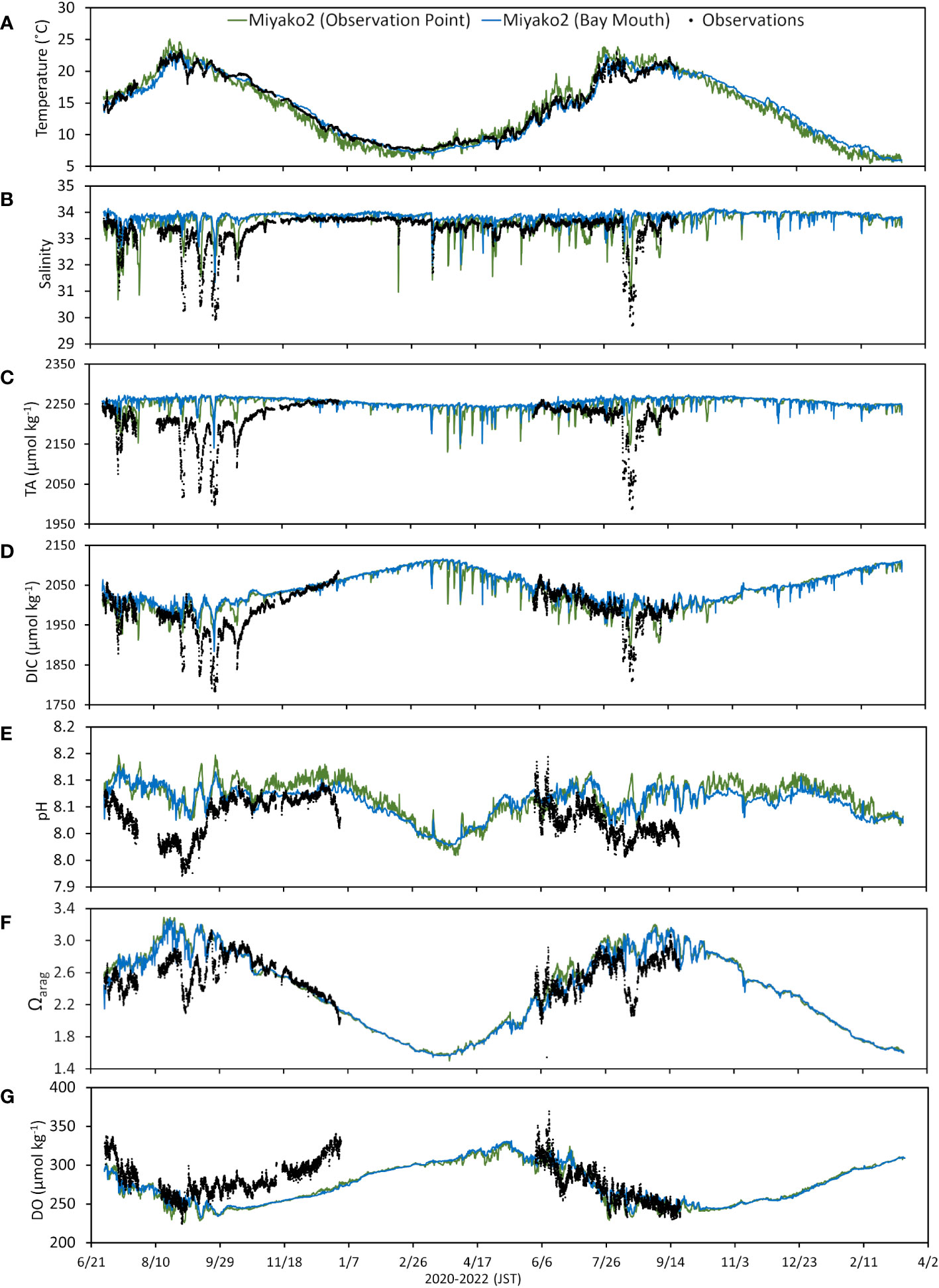
Figure 3 Comparison of results from the present day simulation at the two evaluation points indicated in Figure 1B (close to the FRA observation station and at the mouth of Miyako Bay, at model depths of 1.5 m and 7 m, respectively) with observations for (A) water temperature, (B) salinity, (C) total alkalinity (TA), (D) dissolved organic carbon (DIC), (E) pH, (F) aragonite saturation state (Ω_arag), and (G) dissolved oxygen (DO). Gaps in the observations indicated time periods wherein data was not available due to sensor maintenance or monitoring setup problems.

As for the carbonate parameters, simulated pH and Ω_arag appeared to be at the proper levels and matched observations for some parts of the measurement period. However, the model seemed to have overestimated both parameters during the summer months of 2020 and 2021 (Figures 3E, F). As for DO, the model results follow the seasonal trends seen in the observations, but underestimated observations from late September to December 2020 (Figure 3G).

Aside from the observations from sensors at the FRA observation point, water level data was also available for comparison with model output. This was from a station maintained by the JMA at the location 39.6500° N Latitude and 141.9833° E Longitude for which the data is available for download (https://www.data.jma.go.jp/gmd/kaiyou/db/tide/suisan/suisan.php?stn=MY). Since model outputs for all parameters were set to 6-hourly intervals due to data storage and computational limitations, the present day model was partially rerun specifically to output water level data at hourly intervals for the period July 1 to December 1, 2020. This also allowed a more thorough evaluation through tidal analysis using the T_TIDE analysis package (Pawlowicz et al., 2002). Figure 4A shows the comparison between modeled and observed water level for a selected period, indicating relatively good agreement. The overall pattern of water level changes was properly simulated, although the model had some tendency to slightly underestimate the tidal amplitude. After running a T_TIDE analysis for both observations and model outputs (see Supplementary Material Section 4), the residuals were also obtained and these are compared in Figure 4B. The model residual followed the general long term trend of that of the observations but could not properly resolve some downshifts during some periods. These mismatches likely represent other physical factors affecting the water level trends which the model does not incorporate at present. The tidal analysis also determined the tidal components which contributed most to the local patterns, and the six components with the highest amplitudes (M2, K1, O1, S2, Q1, N2) were the same for both observations and model outputs. Their amplitude and phase values are indicated in Supplementary Table TS2. Although a further comparison of modeled and observed water current velocities would have been ideal, in-situ observation data was not available, and an analysis similar to that done for the water level could not be performed.

FIGURE 4

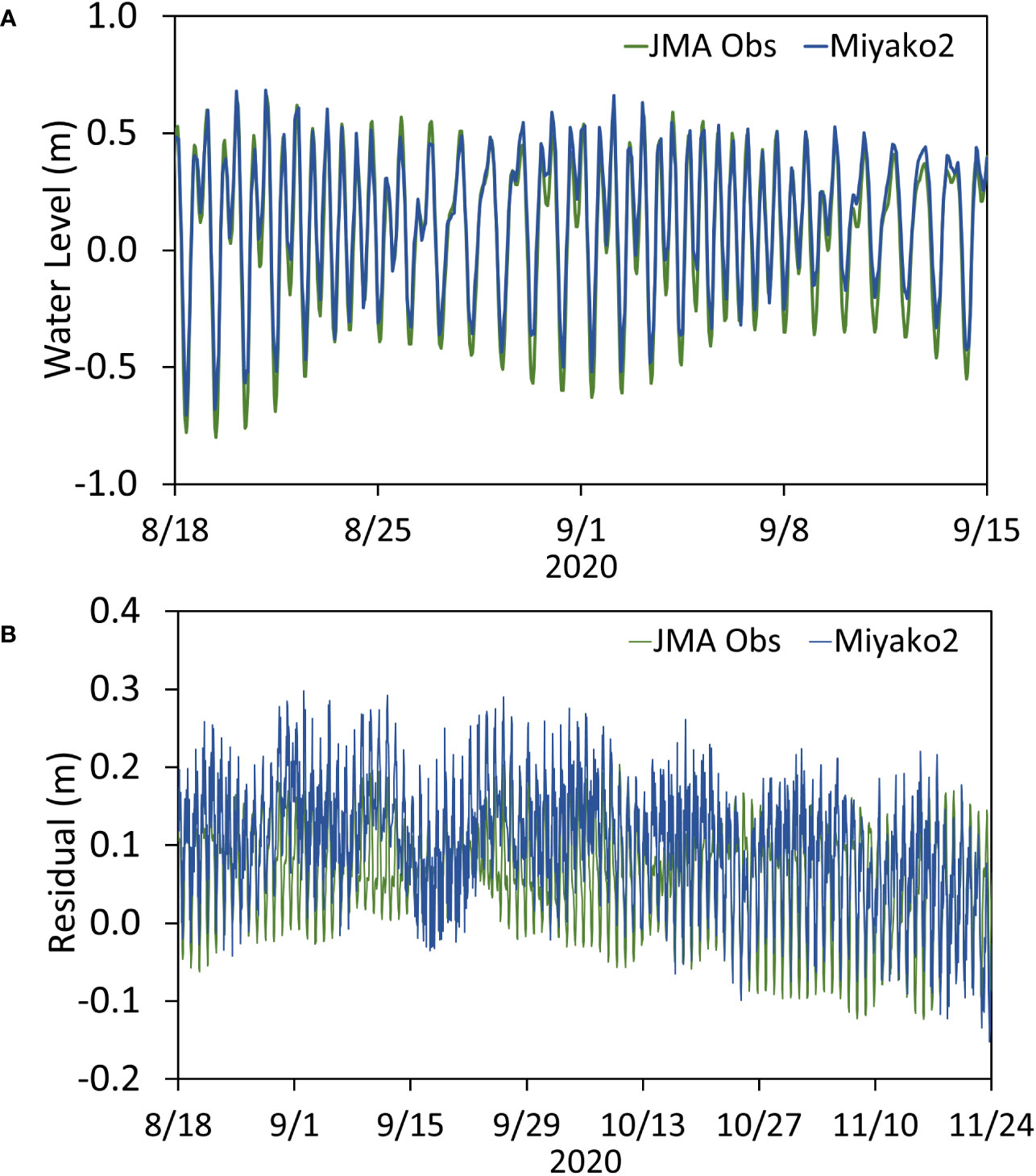
Figure 4 Comparison of observed and modeled water level values at a monitoring point near the mouth of Miyako Bay maintained by the Japan Meteorological Agency (JMA). (A) Comparison of water levels at 1-hour intervals for a selected period spanning 1 month (B) Comparison of residuals obtained after performing tidal analysis over a period of more than 3 months for both JMA observations and Miyako2 model outputs.

To provide a numerical measure of model performance in comparison to the observations, the index of agreement (IA) described in Willmott (1981) was also calculated for each parameter:

$\begin{array}{ll}IA=\frac{{\sum }_{i=1}^n{\left|X{m}_i-X{o}_i\right|}^2}{{\sum }_{i=1}^n{(\left|X{m}_i-\overline{Xo}\right|+\left|X{o}_i-\overline{Xo}\right|)}^2}& (2)\end{array}$

where IA represents the index of agreement ranging from 0 to 1, Xm and Xo represent modeled and observed values, respectively, $\overline{Xo}$ represents the mean of the observed values, and n represents the total number of model versus observation comparisons made. An IA of 1 represents a perfect match between modeled and observed values, while an IA of 0 represents a perfect mismatch. To provide additional quantitative measures of model performance, root mean square error (RMSE), correlation coefficient (CC), bias (BIAS), and relative bias (RBIAS) were also calculated, for which the following equations were used:

$\begin{array}{ll}RMSE=\sqrt{\frac{1}{n}\sum _{i=1}^n{(X{m}_i-X{o}_i)}^2}& (3)\end{array}$

$\begin{array}{ll}CC=\frac{{\sum }_{i=1}^n(X{m}_i-\overline{Xm})(X{o}_i-\overline{Xo})}{\sqrt{{\sum }_{i=1}^n{(X{m}_i-\overline{Xm})}^2{\sum }_{i=1}^n{(X{o}_i-\overline{Xo})}^2}}& (4)\end{array}$

$\begin{array}{ll}BIAS=\frac{1}{n}{\sum }_{i=1}^n(X{m}_i-X{o}_i)& (5)\end{array}$

$\begin{array}{ll}RBIAS=\frac{BIAS}{\overline{Xo}}& (6)\end{array}$

where $\overline{Xm}$ represents the mean of the model values. IA, RMSE, CC, BIAS, and RBIAS values obtained for parameters for which both observations and model outputs were available are listed in Table 1.

TABLE 1

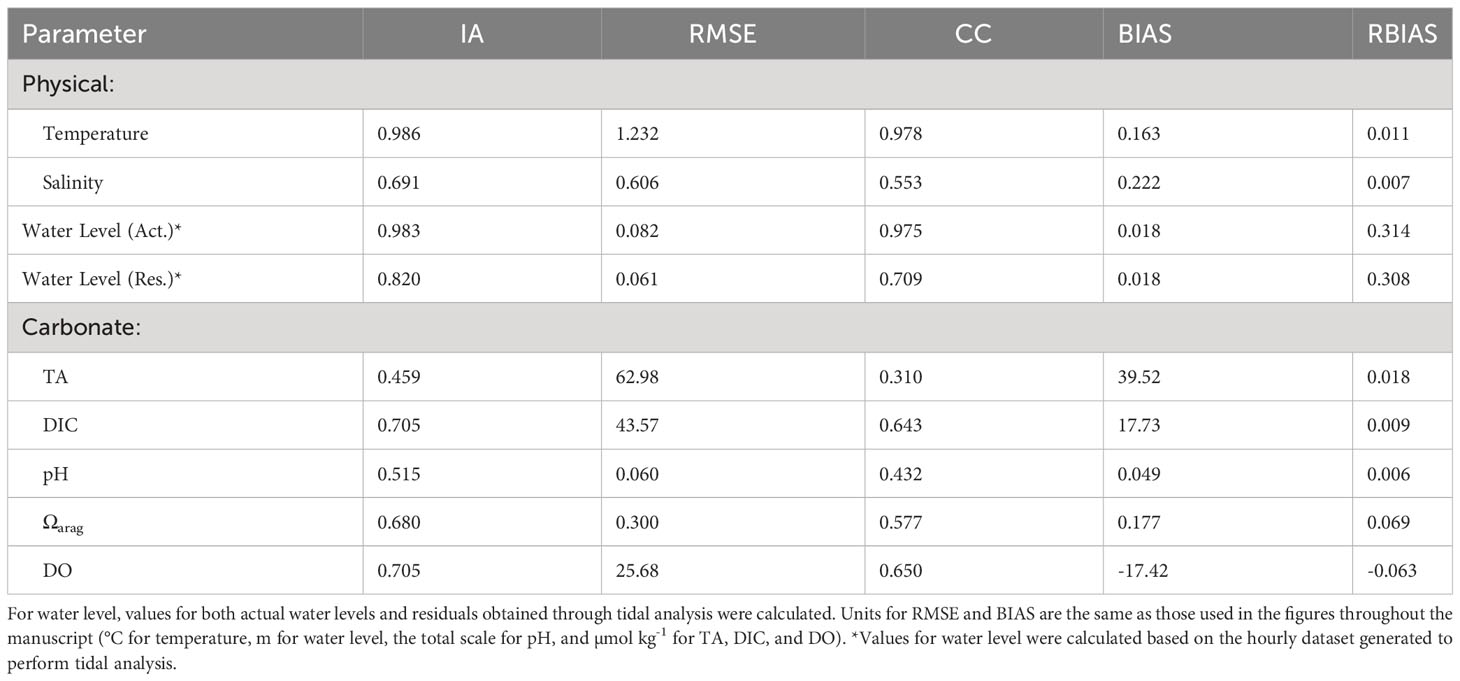
Table 1 Index of agreement (IA) (Willmott, 1981), room mean square error (RMSE), correlation coefficient (CC), bias (BIAS), and relative bias (RBIAS) calculated to compare modeled and observed values of physical and carbonate parameters at the FRA observation point as well as the JMA water level monitoring station.

Relatively high IA values were obtained for water level and temperature (> 0.9). Considerably high indices (IA > 0.6) were also found for salinity, DIC, Ω_arag, and DO. The lowest IA values (~0.5) were found for TA and pH, likely reflecting the drawdowns of these values in the summer to early autumn which the model was not able to accurately capture. These weaknesses in the model are also reflected in the relatively low CC (CC < 0.5) calculated for both TA and pH as well as the relatively high values of RMSE and BIAS for TA. The tendency of the model to overestimate TA and DIC mentioned earlier can be seen in the positive values for BIAS found for both parameters. Model underestimates of DO for some periods are indicated by the negative value for BIAS (Table 1).

As for the tidal analysis of observed and modeled water levels, closer examination of the residuals after the tides were removed revealed that a noticeable diurnal variation still remained in both time-series (Supplementary Figure S4). This suggests that some non-tidal factors may be influencing local water levels. Our initial hypothesis was that this may be possibly caused by trends in the local land-breeze and sea-breeze system as water level peaks occurred during the daytime and troughs during the nighttime for a part of the residual time series. But this trend was not a general one and hence the cause of the diurnal patterns may be a more complex combination of non-tidal factors. Correlations were computed for some meteorological measurements taken at a local weather station (see Supplementary Material Section 4), and although we found a weak but significant correlation for the observed residual time series with the south-north wind component (CC = 0.101; Table TS3), winds alone cannot fully account for the diurnal variation. We have so far found no studies for the area that have previously examined this phenomenon, and hence it may be a topic for further investigation to gain a better understanding of the local hydrodynamics.

To compare signals of much lower frequency, we also applied 37-hour and 73-hour running mean filters to the residual water level time series (Supplementary Figure S5). The resulting time series showed that over the longer term, the modeled water level showed some peaks which did not appear in the observed water level. RMSE calculated for the 37-hour and 73-hour filtered results were 0.044 m and 0.042 m, respectively (Supplementary Table TS4), which quantitatively describe the general discrepancy between observed and modeled water levels. This can likely be attributed to more fine-scale coastal morphological features which the model, even at a 300 m grid resolution, is unable to resolve.

Overall, while there are some characteristics of the observed data which were not reproduced well in the present day simulation, the model was able to properly simulate reasonable values for the important physical and biogeochemical parameters. Hence, performing future scenario testing was considered feasible for this modeling setup in the attempt to assess future oceanic conditions. The differences in observed and modeled results and their timings may also provide possible insights into which kinds of factors may be causing them, and how to incorporate them into the model setup if the mechanisms can be determined and the relevant data obtained.

Observation data for the Omoe observation point has also been collected and compared to model results. However, the data is still of relatively short duration and sensor loss has led to incomplete data for some parameters. The model-observation data comparisons are shown in the Supplementary Material (Section 5, Figure S6) for reference. Temperature and salinity are reproduced quite well. As for DO, the general trend is followed, but similar to the observations near the FRA station, concentration values are underestimated by ~40-50 µmol kg^-1. Also, an abrupt downshift in DO observed from around Dec. 18, 2020 was also not properly reproduced.

3.2 Future scenario comparison

For the results of the future scenario comparison, it is important to note that the FORP model results used to generate model forcing for the scenario testing had been assessed to actually underestimate water temperatures for the general region (mixed water region north of the Kuroshio) by around 1 °C (Nishikawa et al., 2021). Hence, the results for water temperature shown have been increased by 1 °C from the original outputs, and it is this increased temperature that was used in the calculation of the carbonate system parameters pH and Ω_arag. Also, the month of May in all scenario runs was used to give the model a 1-month spin-up duration, and so results for June to April of the following year are considered the main model outputs.

The results of the different scenario simulations are shown in Figure 5 along with the observations from the FRA monitoring point. Since the observations provide the best representation of present day conditions at the Miyako study site, they could also be considered an appropriate basis of comparison for the scenario run results. Simulated seawater temperatures were notably higher than observed values, as might be expected, for the RCP 8.5 scenario for the end of the century, which also had the highest temperature values overall (Figure 5A). For the RCP 2.6 scenario, simulated temperatures were at times higher, similar to, or lower than observed. The RCP2.6 scenario results also looked similar to those obtained for the RCP8.5 results for the 2050s. In the historical scenario, simulated temperatures were significantly lower than observed in general, except for the early summer months where they were quite similar. This is quite reasonable given that the historical scenario represents conditions around 20 years prior to the present day. In terms of the salinity outputs, the historical scenario also had the best match with the observed values, but in general all scenarios appear to have salinity values around 0.5 greater than observed (Figure 5B). The results for TA show similar results among the different scenarios (Figure 5C), but this is an expected result as the same TA boundary conditions were used in all the scenarios. On the other hand, simulated results for DIC showed significant variation between scenarios, reflecting the boundary condition settings which were based on scenario runs performed using the larger scale MIROC-ESM biogeochemical model (Watanabe et al., 2011). The historical simulation results for DIC closely followed the observed values, with larger DIC values as can be expected for the end of century RCP scenarios (Figure 5D).

FIGURE 5

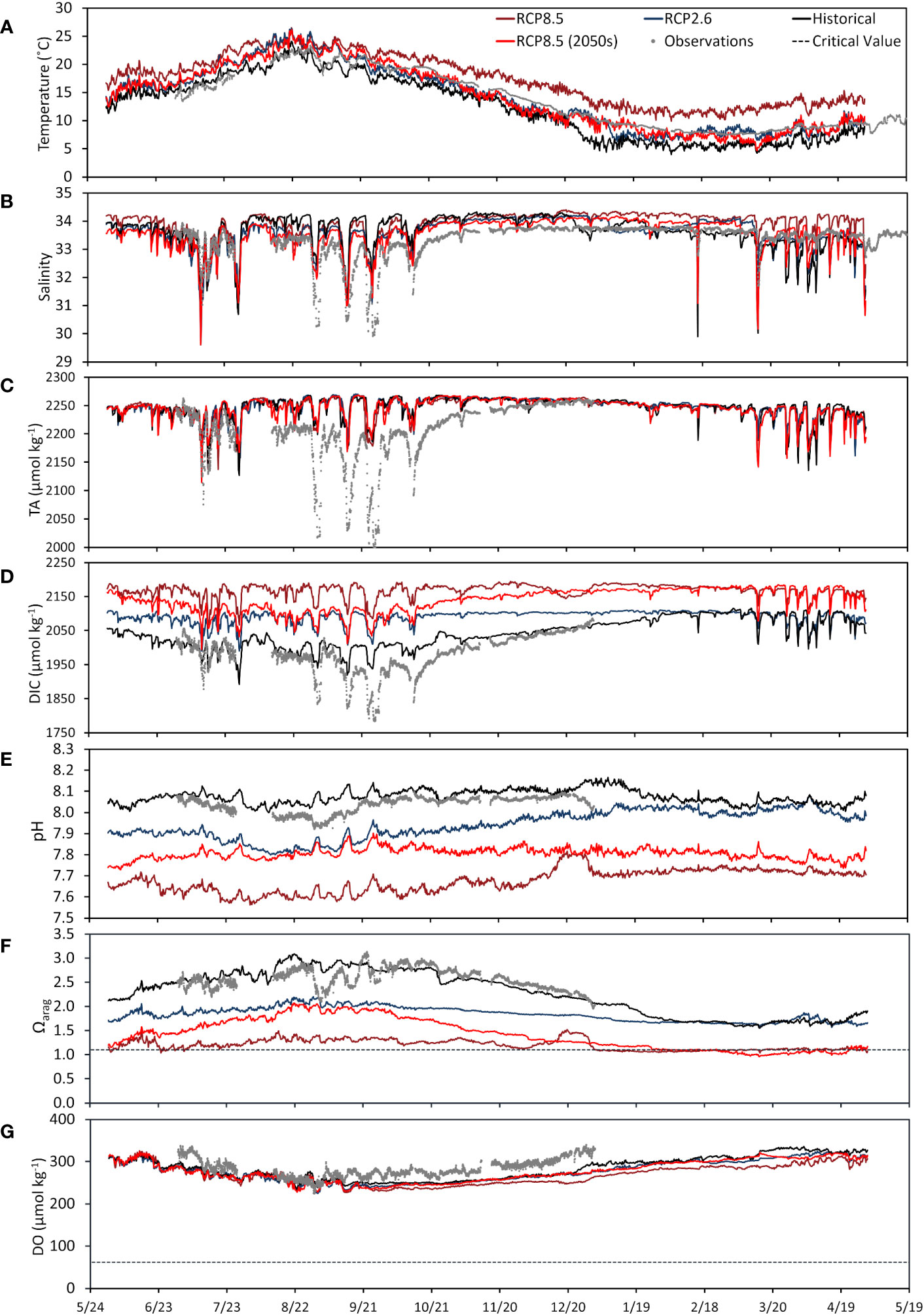
Figure 5 Comparison of results from the historical and future projection simulations at the model evaluation point close to the FRA station. Observations are also plotted for reference. (A) water temperature (with 1 °C increase), (B) salinity, (C) total alkalinity (TA), and (D) dissolved organic carbon (DIC), (E) pH, (F) aragonite saturation state (Ω_arag), and (G) dissolved oxygen (DO). Relevant critical values for calcifying shellfish for Ω_arag (1.1; Onitsuka et al., 2018), and for marine organisms for DO (62 μmol kg^-1; Vaquer-Sunyer and Duarte, 2008) are shown as a dotted black line in (F, G), respectively. The pH and Ω_arag were calculated using water temperature values increased by 1 °C.

The results for parameters indicating acidification are shown in Figures 5E, F, along with a recognized threshold for Ω_arag (1.1; Onitsuka et al., 2018). The historical simulation results appear reasonable as the pH and Ω_arag trends generally follow those of the observations, apart from the rapid drops during some parts of the year (Figures 5E, F). On the other hand, the future scenarios show significantly decreased pH and Ω_arag for most parts of the year, particularly in the RCP 8.5 results. From the results of the future scenario for the 2050s under RCP 8.5 conditions, it can be seen that even by the middle of the century, the threshold Ω_arag value may already be reached during some parts of the year, from late winter to spring. Although this shows the case for the worst case of anthropogenic CO₂ emissions, it may be necessary to take precaution and increase the pace of determining and implementing proper mitigation and adaptation strategies. For DO however, although differences in scenarios can be seen, and the simulated DO is lowest in the end of century RCP 8.5 results, the decrease in concentration is not so dramatic and appear to be at the level of or less than present day fluctuations in observed DO (Figure 5G). Unlike for temperature and DIC, the same initial and boundary conditions were used for all scenarios for DO because we were unable to find an appropriate dataset. Suitable datasets were not available due to continued difficulties in projecting future DO trends in general; these difficulties are highlighted by differences in modeled versus observational trends as well as disagreements in model projected spatial patterns of oxygen decline (Breitburg et al., 2018). The differences among the scenarios in our results likely reflects the influence of decreased oxygen solubility with the rise in water temperature, even if the same DO initial and boundary conditions were used. A recognized threshold for DO (62 μmol kg^-1; Vaquer-Sunyer and Duarte, 2008) is also indicated, and although model results are way above the threshold, further consideration of the DO initial and boundary conditions will be necessary in future versions of the setup to enable a more appropriate assessment.

To provide a clearer comparison, the scenario results shown in Figure 5 were also compiled into monthly averages, and these are shown in Figure 6. As has been mentioned, simulated temperatures appear to be very similar between the RCP2.6 end of century and RCP8.5 middle of the century scenario. Salinity appears highest for the RCP8.5 end of century scenario, particularly for the first few months of the year. For pH and Ω_arag, both RCP8.5 scenarios simulations indicate alarming levels for most of the year.

FIGURE 6

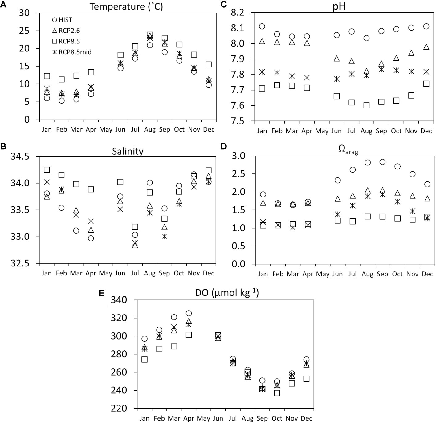
Figure 6 Monthly averages of the time-series outputs shown in Figure 5 for selected parameters comparing the different scenarios. As the month of May was used for model spin-up, model outputs for this month are omitted in the plots. (A) water temperature, (B) salinity, (C) pH, (D) Ω_arag, and (E) DO.

3.3 Bias correction

As a way to minimize the effects of FORP model biases on the future scenario comparisons, a bias correction procedure modified from that used in Fujii et al. (2021), which was adapted from Yara et al. (2011), was applied to provide alternative sets of future projections. Although FORP results may be biased for certain variables in specific regions, since a similar setup is used to run the historical, middle-of-century, and end-of-century scenarios, comparing FORP modeling results among themselves may be a reasonable way to estimate rates of change for variables of interest. In this case, modeling results of the historical and future scenarios were compiled for water temperature, DIC, DO, and annual rates of change were calculated for the RCP 2.6 and RCP 8.5 scenario results relative to the historical scenario results. Each RCP scenario represented conditions either 50 or 99 years after the historical scenario, and hence annual rates of change were calculated using a simple linear calculation for each parameter. The model outputs were at 6-hourly time steps, and hence it was possible to obtain values for each time step.

To obtain bias-corrected future projections, two base results were used. In the first version, the calculated rates of change were applied to the results of the present day (HYCOM-forced) simulation. In the second version, the calculated rates of change were applied directly to the observations taken at the FRA station. As both the present day simulation and the observations (mainly 2020-2021) are at a time frame approximately 20 years after the historical scenario (2000-2001), this was taken into account in the calculation for future projections, which used 80 years and not 100 years in the estimation of future parameter values. The calculation was conducted as follows:

$\begin{array}{ll}{\text{Φ}}_{\text{f}}={\text{Φ}}_{\text{p}}+\text{ΔΦ}& (7)\end{array}$

$\begin{array}{ll}\text{ΔΦ}={\mu }_{rate} \times n_{yr} & (8)\end{array}$

where for a specific parameter Φ (water temperature, DIC, or DO), Φ_f is the future projected value, Φ_p is the base value, either present day simulation or observation, µ_rate is the yearly rate of change of the parameter (e.g., Celsius degrees per year), and n_yr is the number of years after the present time for which the projected value is being computed for. As pH and Ω_arag are not directly calculated in the model, future projected values were calculated using the projected values for water temperature and DIC calculated using equations (7) and (8), and appropriate values for salinity and TA within the CO2SYS for Excel program (Pierrot et al., 2006). For the present day simulation case, RCP 2.6 and RCP 8.5 scenario results for salinity and TA were used. For the observations case, as no reasonable future projection data sets for salinity or TA could be found at present, observed values for salinity and TA were used.

The results of the bias-corrected future projection calculations are shown in Figures 7, 8. Compared to the scenario modeling results (Figure 5), the bias-corrected projections of ocean acidification appear relatively less severe under the two RCP 8.5 scenarios in that the threshold Ω_arag value (Ω_arag = 1.1) is reached or exceeded for shorter time periods. Nevertheless, both versions of the bias-corrected projections show that the threshold may be reached during certain parts of the year, which is still cause for concern. Unfortunately, carbonate parameter observations were not available to assess winter and spring season trends using this bias correction approach.

FIGURE 7

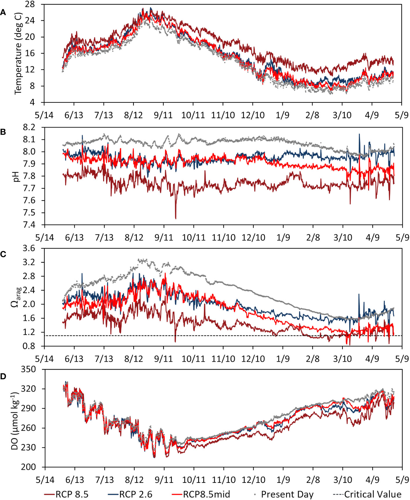
Figure 7 Comparison of bias-corrected future projection calculations using output from the present day (HYCOM-forced) model simulation as base conditions for (A) water temperature, (B) pH, (C) Ω_arag, and (D) DO, with relevant critical value indicated for (C) Ω_arag (1.1; Onitsuka et al., 2018). Results greatly exceeded the critical value for DO (62 μmol kg^-1; Vaquer-Sunyer and Duarte, 2008) and hence it is not shown in (D).

FIGURE 8

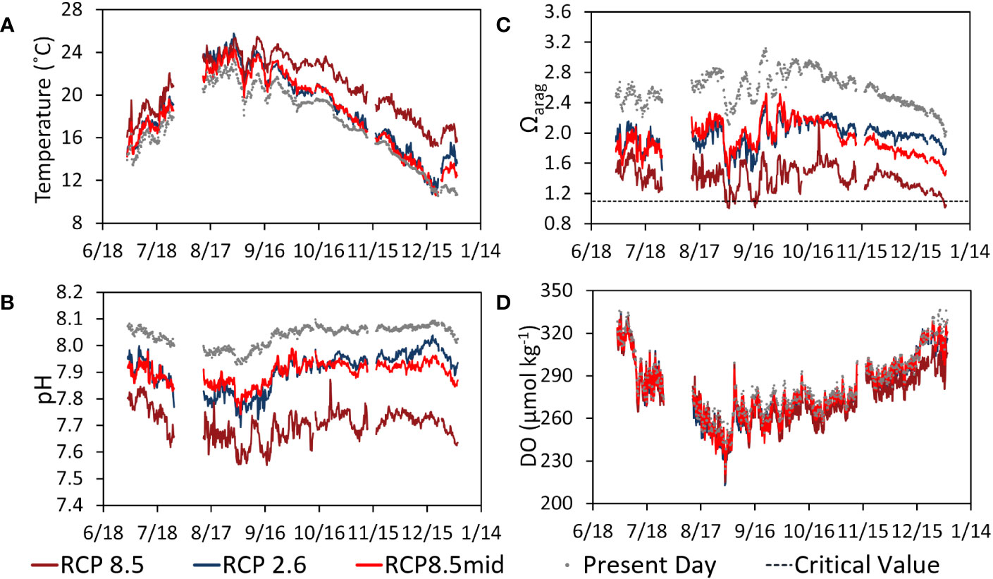
Figure 8 Same as Figure 7 but for bias-corrected future projection calculations using the observed values taken at the FRA monitoring point as base conditions for (A) water temperature, (B) pH, (C) Ω_arag, and (D) DO, with relevant critical value indicated for (C) Ω_arag (1.1; Onitsuka et al., 2018). Results greatly exceeded the critical value for DO (62 μmol kg^-1; Vaquer-Sunyer and Duarte, 2008) and hence it is not shown in (D).

In terms of the weaknesses of this approach, although giving reasonable results, the present day simulation was not able to capture some of the trends seen in the observations. On the other hand, logistical problems with sensors have led to observations being unavailable for some parts of the measurement period. This prevented us from obtaining a longer time-series of bias-corrected results based on the observation dataset (Figure 8). Nevertheless, the bias-corrected results taken together can potentially be helpful, and the future projections as a whole suggest that coastal waters approaching critical levels of Ω_arag may be a more common occurrence under RCP 8.5 conditions.

4 Discussion

4.1 Model evaluation and possible implications

In spite of the limitations in the modeling approach we developed, the results at hand may still be used to obtain some helpful insights. Experimentally based critical values for Ω_arag vary based on the calcifying organism species at values in the range 1.1-1.5 (e.g., Waldbusser et al., 2015; Zhan et al., 2016; Onitsuka et al., 2018; Bednaršek et al., 2019). However, for this particular study it may be most appropriate to highlight the critical value for the locally grown Ezo Abalone species Haliotis discus hannai which was determined to be an Ω_arag value of 1.1 in Onitsuka et al. (2018). Larval abalone exposed to values of 1.1 or lower were found to have decreased shell lengths and higher malformation rates, suggesting the possible occurrence of negative impacts under future ocean acidification. Based on the future projections performed in this study, values of Ω_arag close to this critical value may likely be approached for part of or most of the year under the end-of-century RCP8.5 scenario (Figures 5F, 7C, 8C). Another commercially important local species is the Pacific oyster (Crassostrea gigas) for which a previous study conducted outside Japan has suggested an even higher threshold value of Ω_arag =1.5 (Waldbusser et al., 2015). This threshold is exceeded for an even longer duration in the end-of-century RCP8.5 scenario and becomes a significant concern even for the middle-of-century RCP8.5 scenario even in the bias-corrected results (Figures 5F, 7C, 8C). While there are aspects of the modeling approach used that may need improvement, these results stress the need to seriously consider possible mitigation and adaptation approaches to better safeguard Ezo Abalone, Pacific oyster, and other economically important calcifying marine organisms in the region.

As for DO, the insufficiency of the future DO initial and boundary conditions in our scenario runs prevent us from making a thorough discussion about possible future conditions. In terms of the present day, observed and simulated DO values were very much above a recognized median lethal oxygen concentration (LC₅₀) of 62 μmol kg^-1 (2.05 mg l^-1), which was the mean LC₅₀ found for all marine organisms considered in Vaquer-Sunyer and Duarte (2008). The same paper however recommends setting a higher threshold of 140 μmol kg^-1 (4.6 mg l^-1), which represents the 90^th percentile of the distribution of mean LC₅₀, so as to more cautiously ensure marine biodiversity conservation. Moreover, a recent study on larvae and embryo of the Japanese whiting (Sillago japonica), a locally important fisheries species, indicate an LC₅₀ in the range 90-93 μmol kg^-1 at a pH of 7.8 (Yorifuji et al., 2023), which is at the pH range predicted for the end-of-century RCP8.5 scenario. These would be important considerations for assessing the results of improved versions of this model setup in the future. Some studies have also suggested that even small decreases in DO (<10 μmol kg^-1) are likely to influence important fishery species (e.g., Stortini et al., 2017; Breitburg et al., 2018). Although the variation in DO results in our scenario runs for this study may not be reliably used to project future conditions, it may indicate at least the potential of our model setup to capture even relatively small changes in DO.

It also must be recognized that our current model setup does not consider possible land use changes which may affect the nutrient input loads from terrestrial areas to the coast. The lack of observation data within Miyako Bay itself makes us further unable to formulate more concrete hypotheses about future DO conditions, but the present day example of Tokyo Bay which is surrounded by a highly urbanized area may serve as a caveat. Highly eutrophic conditions due to the large amounts of nutrient loading has led to the progression of both ocean acidification and hypoxia, and even anoxia during some parts of the year (Yamamoto-Kawai et al., 2015; Yamamoto-Kawai et al., 2021). While Miyako Bay may not really go the way of Tokyo Bay in terms of urbanization and population increase, it is nevertheless important to stress awareness of the conditions through which hypoxia may develop and threaten the local marine ecosystem.

4.2 Towards improving the present approach

In spite of our approach demonstrating the capability to reproduce important physical and biogeochemical parameters related to ocean acidification and deoxygenation as well as run future scenarios, as the obtained results indicate, some work towards its improvement is necessary. The observation-model mismatches for some periods in the salinity suggest the presence of more local sources of freshwater. While we presently have no evidence, submarine groundwater discharge (SGD) in the area may need to be more properly characterized and incorporated into the model setup. For the historical and future scenarios, to adhere more closely to what are considered best practices in the modeling community at large (e.g., Drenkard et al., 2021), it also may be preferrable to run the simulation for a longer period to look into possible interannual variations. However, running hydrodynamic-ecosystem models at a relatively high spatial resolution comes at a significant computational cost (e.g., Nishikawa et al., 2021) and this is left for future work after additional improvements have been made to the model setup.

It must also be recognized that in terms of complexity, the approach we used is less comprehensive than sophisticated modeling setups which have been developed for some particular regions, such as the Salish Sea (Khangaonkar et al., 2018, Khangaonkar et al., 2021) and the Gulf of Saint Lawrence (Lavoie et al., 2021). Such large scale cooperative modeling investigations involving various research groups as well as government institutions with access to comprehensive observational data sets are indeed closer to the ideal. However, for areas where observation data as well as financial and logistical support are more limited, alternative approaches may need to be explored. The regional to local focus we have employed also allows us to potentially consult more closely with the local community in order to further develop and improve the model setup and utilize it to help address the most relevant local concerns. It may form part of an integrated framework involving various stakeholders, including scientists of various disciplines, local government, industry representatives, and the general public, with the aim of developing the most effective plans to address ocean acidification and deoxygenation (e.g. Breitburg et al., 2018), and promote the growth of local citizen science efforts. This is perhaps especially true for an island country like Japan with numerous coastal communities located relatively far from urban centers where most resources and manpower are concentrated. The current model setup also lacks a sophisticated benthic layer ecosystem component (e.g. Sohma et al., 2008), and this is left for future work in combination with additional monitoring efforts directed more to the inner parts of Miyako Bay.

In spite of the problems and logistical challenges encountered which led to gaps in the dataset as well as being limited to a single monitoring point, a very important part of this work was the availability of in situ observations with which to compare model results to and provide some assessment of model performance. While ecosystem models may be potentially useful tools in the continuing study of global warming, ocean acidification, and deoxygenation and their impacts on the marine environment, they go hand in hand with essential monitoring efforts. As has been shown in Fujii et al. (2021) and this present study, targeted modeling and monitoring approaches represent a viable strategy to help assess the situation in coastal areas of interest in order to properly determine the most appropriate adaptation and mitigation measures.

5 Conclusion

In this study we have attempted to develop a combined hydrodynamic and marine ecosystem modeling approach to study ocean acidification and deoxygenation in coastal areas. We first developed a present day simulation which we were able to validate through comparisons with in situ time-series observations. The simulation was able to reproduce the general features of observed physical and biochemical parameters, except for some rapid decreases in salinity, pH and aragonite saturation state (Ω_arag). This suggests that other local factors, such as submarine groundwater discharge, may need to be introduced into the model. River inputs may be also underestimated, and hence more accurate parameterizations are necessary. Furthermore, the extra step has been taken to attempt scenario testing of historical and future scenarios based on what is presently the best physical forcing dataset available at the resolution necessary to study coastal phenomena along the coasts of Japan (FORP; Nishikawa et al., 2021). And although the relatively short run durations (~1 year) are a limitation, results of the future projections suggest potentially significant impacts of global warming and ocean acidification on calcifying organisms under the RCP 8.5 scenario. In particular, it is feared that by the end of the century, values of Ω_arag would approach a critical level for calcifying organisms (Ω_arag< 1.1) throughout the year under which decreased larval shell lengths and malformation have been observed experimentally for the commercially important Ezo Abalone species (Onitsuka et al., 2018). Much effort continues to be devoted to the improvement of global future projections for different emission scenarios (Kwiatkowski et al., 2020), and downscaling such large-scale model results can always be an avenue for further development of the approach described in this study. And though some aspects of the model setup and the overall approach need further improvement, the results obtained may already be helpful for gaining insights on what would be viable adaptation and mitigation strategies to conserve the local marine ecosystem from stresses to be brought about by future ocean warming, acidification, and deoxygenation.

Data availability statement

The raw data supporting the conclusions of this article will be made available by the authors, without undue reservation.

Author contributions

LB, MF, TO contributed to the study conception and design. LB, MF, and TO designed the modeling approach, LB set up and ran the models, TO and MF collected, processed, and provided the monitoring data. LB wrote the first draft of the manuscript, and all authors contributed to subsequent revisions. All authors contributed to the article and approved the submitted version.

Funding

This study was conducted by Theme 4 of the Advanced Studies of Climate Change Projection (SENTAN Program) Grant Number JPMXD0722678534 supported by the Ministry of Education, Culture, Sports, Science and Technology (MEXT), Japan, and the Study of Biological Effects of Acidification and Hypoxia (BEACH) of the Environment Research and Technology Development Fund Grant Number JPMEERF20202007 of the Environmental Restoration and Conservation Agency of Japan. This study utilized the Future Ocean Regional Projection (FORP) dataset, which was produced by the Japan Agency for Marine-Science and Technology (JAMSTEC) under the Social Implementation on Climate Change Adaptation Technology (SI-CAT) project (Grant Number: JPMXD0715667163) of the MEXT, Japan. The FORP-JPN02 dataset provided by JAMSTEC was utilized in this research, which was also collected and provided under the Data Integration and Analysis System (DIAS), which was developed and operated by a project supported by the MEXT, Japan.

Acknowledgments

We thank Yukihiro Nojiri and Hideaki Nakata for their fruitful discussions, and Wakako Takeya for the support. To help facilitate model initial and boundary condition processing, open-source ROMS modeling tools available from https://zenodo.org/record/7432028, https://www.myroms.org/projects/src/wiki, https://www.croco-ocean.org/download/croco-project, and https://github.com/NakamuraTakashi were adapted for use in our work.

Conflict of interest

The authors declare that the research was conducted in the absence of any commercial or financial relationships that could be construed as a potential conflict of interest.

Publisher’s note

All claims expressed in this article are solely those of the authors and do not necessarily represent those of their affiliated organizations, or those of the publisher, the editors and the reviewers. Any product that may be evaluated in this article, or claim that may be made by its manufacturer, is not guaranteed or endorsed by the publisher.

Supplementary material

The Supplementary Material for this article can be found online at: https://www.frontiersin.org/articles/10.3389/fmars.2023.1174892/full#supplementary-material

References

Aumont O., Bopp L. (2006). Globalizing results from ocean in situ iron fertilization studies. Global Biogeochem. Cycles 20, GB2017. doi: 10.1029/2005GB002591

CrossRef Full Text | Google Scholar

Bates N. R., Astor Y. M., Church M. J., Currie K., Dore J. E., González-Dávila M., et al. (2014). A time-series view of changing ocean chemistry due to ocean uptake of anthropogenic CO₂ and ocean acidification. Oceanography 27 (1), 126–141. doi: 10.5670/oceanog.2014.16

CrossRef Full Text | Google Scholar

Bednaršek N., Feely R. A., Howes E. L., Hunt B. P. V., Kessouri F., León P., et al. (2019). Systematic review and meta-analysis toward synthesis of thresholds of ocean acidification impacts on calcifying pteropods and interactions with warming. Front. Mar. Sci. 6. doi: 10.3389/fmars.2019.0022

CrossRef Full Text | Google Scholar

Breitburg D., Levin L. A., Oschlies A., Grégoire M., Chavez F. P., Conley D. J., et al. (2018). Declining oxygen in the global ocean and coastal waters. Science 359, eaam7240. doi: 10.1126/science.aam7240

PubMed Abstract | CrossRef Full Text | Google Scholar

Cummings V., Hewitt J., Van Rooyen A., Currie K., Beard S., Thrush S., et al. (2011). Ocean Acidification at High Latitudes: Potential Effects on Functioning of the Antarctic Bivalve Laternula elliptica. PloS One 6 (1), e16069. doi: 10.1371/journal.pone.0016069

PubMed Abstract | CrossRef Full Text | Google Scholar

DePasquale E., Baumann H., Gobler C. J. (2015). Vulnerability of early life stage Northwest Atlantic forage fish to ocean acidification and low oxygen. Mar. Ecol. Prog. Ser. 523, 145–156. doi: 10.3354/meps11142

CrossRef Full Text | Google Scholar

Doney S. C., Fabry V. J., Feely R. A., Kleypas J. A. (2009). Ocean acidification: the other CO₂ problem. Ann. Rev. Mar. Sci. 1, 169–192. doi: 10.1146/annurev.marine.010908.163834

PubMed Abstract | CrossRef Full Text | Google Scholar

Drenkard E. J., Stock C., Ross A. C., Dixon K. W., Adcroft A., Alexander M., et al. (2021). Next-generation regional ocean projections for living marine resource management in a changing climate. ICES J. Mar. Sci. 78, 1969–1987. doi: 10.1007/s12237-013-9594-3

CrossRef Full Text | Google Scholar

Duarte C. M., Hendriks I. E., Moore T. S., Olsen Y. S., Steckbauer A., Ramajo L., et al. (2013). Is ocean acidification an open-ocean syndrome? Understanding anthropogenic impacts on seawater pH. Estuaries Coasts 36, 221–236. doi: 10.1007/s12237-013-9594-3

CrossRef Full Text | Google Scholar

Fennel K., Testa J. M. (2019). Biogeochemical controls on coastal hypoxia. Ann. Rev. Mar. Sci. 11, 105–130. doi: 10.1146/annurev-marine-010318-095138

PubMed Abstract | CrossRef Full Text | Google Scholar

Fujii M., Hamanoue R., Bernardo L. P. C., Ono T., Dazai A., Oomoto S., et al. (2023). Observed and projected impacts of coastal warming, acidification and deoxygenation on Pacific oyster (Crassostrea gigas) farming: A case study in the Hinase Area, Okayama Prefecture and Shizugawa Bay, Miyagi Prefecture, Japan. Biogeosciences (in revision).

Google Scholar

Fujii M., Takao S., Yamaka T., Akamatsu T., Fujita Y., Wakita M., et al. (2021). Continuous monitoring and future projection of ocean warming, acidification, and deoxygenation on the subarctic coast of Hokkaido, Japan. Front. Mar. Sci. 8. doi: 10.3389/fmars.2021.590020

CrossRef Full Text | Google Scholar

Fujita Y. (2021). Assessing and projecting the impacts of ocean acidification on the sea urchin Strongylocentrotus nudus. Master’s thesis (Hokkaido University: Graduate School of Environmental Science), 67.

Google Scholar

Garcia H. E., Locarnini R. A., Boyer T. P., Antonov J. I., Baranova O. K., Zweng M. M., et al. (2010a). World ocean atlas 2009, volume 3: dissolved oxygen, apparent oxygen utilization, and oxygen saturation. Ed. Levitus S. (Washington, D.C.: NOAA Atlas NESDIS 70, U.S. Government Printing Office), 344.

Google Scholar

Garcia H. E., Locarnini R. A., Boyer T. P., Antonov J. I., Zweng M. M., Baranova O. K., et al. (2010b). World Ocean Atlas 2009, Volume 4: Nutrients (phosphate, nitrate, silicate). Ed. Levitus S. (Washington, D.C.: NOAA Atlas NESDIS 71, U.S. Government Printing Office), 398.

Google Scholar

Gattuso J.-P., Hansson L. (2011). “Ocean acidification: background and history,” in Ocean acidification. Eds. Gattuso J.-P., Hansson L. (Oxford University Press Inc., New York), 1–20.

Google Scholar

Gobler C. J., Baumann H. (2016). Hypoxia and acidification in ocean ecosystems: coupled dynamics and effects on marine life. Biol. Lett. 12, 20150976. doi: 10.1098/rsbl.2015.0976

PubMed Abstract | CrossRef Full Text | Google Scholar

Haidvogel D. B., Arango H. G., Hedstrom K., Beckmann A., Malanotte-Rizzoli P., Shchepetkin A. F. (2000). Model evaluation experiments in the North Atlantic Basin: Simulations in nonlinear terrain-following coordinates. Dyn. Atmos. Oceans 32, 239–281. doi: 10.1016/S0377-0265(00)00049-X

CrossRef Full Text | Google Scholar

Intergovernmental Panel on Climate Change (IPCC). (2019). IPCC special report on the ocean and cryosphere in a changing climate. Eds. Pörtner H.-O., Roberts D. C., Masson-Delmotte V., Zhai P., Tignor M., Poloczanska E., Mintenbeck K., Alegría A., Nicolai M., Okem A., Petzold J., Rama B., Weyer N. M. (Cambridge, UK and New York, NY, USA: Cambridge University Press), 755. doi: 10.1017/9781009157964

CrossRef Full Text | Google Scholar

Jiang L.-Q., Carter B. R., Feely R. A., Lauvset S. K., Olsen A. (2019). Surface ocean pH and buffer capacity: past, present and future. Sci. Rep. 9, 18624. doi: 10.1038/s41598-019-55039-4

PubMed Abstract | CrossRef Full Text | Google Scholar

Joshi A. P., Warrior H. V. (2022). Comprehending the role of different mechanisms and drivers affecting the sea-surface pCO2 and the air-sea CO2 fluxes in the Bay of Bengal: A modeling study. Mar. Chem. 243, 104120. doi: 10.1016/j.marchem.2022.104120

CrossRef Full Text | Google Scholar

Jullien S., Caillaud, Benshila M. R., Bordois L. Cambon G., Dumas F., Le Gentil S., et al. (2019). Coastal and Regional Ocean COmmunity (CROCO) modeling system technical and numerical documentation. doi: 10.5281/zenodo.7400759

CrossRef Full Text | Google Scholar

Keeling R. F., Körtzinger A., Gruber N. (2010). Ocean deoxygenation in a warming world. Ann. Rev. Mar. Sci. 2 (1), 199–229. doi: 10.1146/annurev.marine.010908.163855

PubMed Abstract | CrossRef Full Text | Google Scholar

Khangaonkar T., Nugraha A., Premathilake, Keister L. J., Borde A. (2021). Projections of algae, eelgrass, and zooplankton ecological interactions in the inner Salish Sea – for future climate, and altered oceanic states. Ecol. Model. 441, 109420. doi: 10.1016/j.ecolmodel.2020.109420

CrossRef Full Text | Google Scholar

Khangaonkar T., Nugraha A., Xu W., Long W., Bianucci L., Ahmed A., et al. (2018). Analysis of hypoxia and sensitivity to nutrient pollution in Salish Sea. J. Geophys. Res.-Oceans 123, 4735–4761. doi: 10.1029/2017JC013650

CrossRef Full Text | Google Scholar

Kobayashi J. (1961). A chemical study on the average quality and characteristics of river waters of Japan. Nougou Kenkyu 48 (2), 63–106.

Google Scholar

Kroeker K. J., Kordas R. L., Crim R., Hendriks I. E., Ramajo L., Singh G. S., et al. (2013). Impacts of ocean acidification on marine organisms: quantifying sensitivities and interaction with warming. Glob. Change Biol. 19, 1884–1896. doi: 10.1111/gcb.12179

CrossRef Full Text | Google Scholar

Kwiatkowski L., Torres O., Bopp L., Aumont O., Chamberlain M., Christian J. R., et al. (2020). Twenty-first century ocean warming, acidification, deoxygenation, and upper-ocean nutrient and primary production decline from CMIP6 model projections. Biogeosciences 17, 3439–3470. doi: 10.5194/bg-17-3439-2020

CrossRef Full Text | Google Scholar

Lavoie D., Lambert N., Starr M., Chassé J., Riche O., Le Clainche Y., et al. (2021). The gulf of st. Lawrence biogeochemical model: A modelling tool for fisheries and ocean management. Front. Mar. Sci. 8. doi: 10.3389/fmars.2021.73226

CrossRef Full Text | Google Scholar

Lewis E., Wallace D., Allison L. J. (1998). Program developed for CO₂ system calculations, ORNL/CDIAC-105 (Oak Ridge Natl. Lab). doi: 10.2172/639712

CrossRef Full Text | Google Scholar

Locarnini R. A., Mishonov A. V., Antonov J. I., Boyer T. P., Garcia H. E., Baranova O. K., et al. (2010). World ocean atlas 2009, volume 1: temperature. Ed. Levitus S. (Washington, D.C.: NOAA Atlas NESDIS 68, U.S. Government Printing Office), 184.

Google Scholar

Melzner F., Thomsen J., Koeve W., Oschlies A., Gutowska M. A., Bange H. W., et al. (2013). Future ocean acidification will be amplified by hypoxia in coastal habitats. Mar. Biol. 160, 1875–1888. doi: 10.1007/s00227-012-1954-1

CrossRef Full Text | Google Scholar

Murakami T., Ogasawara T., Shimokawa S. (2015). Numerical analysis of sediment transport in Miyako Bay, Iwate, Japan. J. Jpn. Soc Civ. Eng. Ser. (Coastal Engineering) 71, I_1213–I_1218. (In Japanese with English abstract). doi: 10.2208/kaigan.71.I_1213

CrossRef Full Text | Google Scholar

Nishikawa S., Wakamatsu T., Ishizaki H., Sakamoto S., Tanaka Y., Tsujino H., et al. (2021). Development of high-resolution future ocean regional projection datasets for coastal applications in Japan. Prog. Earth Planet. Sci. 8, 7. doi: 10.1186/s40645-020-00399-z

CrossRef Full Text | Google Scholar

Okada T., Maruya Y., Nakayama K., Iseri E. (2014). A Study on restoration of eelgrass (Zostera marina) damaged by tsunami in Miyako Bay. J. Jpn. Soc Civ. Eng. Ser. 70, I_1186–I_1190. (in Japanese with English abstract). doi: 10.2208/kaigan.70.I_1186

CrossRef Full Text | Google Scholar

Onitsuka T., Takami H., Muraoka D., Matsumoto Y., Nakatsubo A., Kimura R., et al. (2018). Effects of ocean acidification with pCO₂ diurnal fluctuations on survival and larval shell formation of Ezo abalone, Haliotis discus hannai. Mar. Environ. Res. 134, 28–36. doi: 10.1016/j.marenvres.2017.12.015

PubMed Abstract | CrossRef Full Text | Google Scholar

Ono T., Muraoka D., Hayashi M., Yorifuji M., Dazai A., Omoto S., et al. (2023). Short-term variation of pH in seawaters around Japan coastal areas: Its characteristics and forcings. Biogeosciences (in revision).

Google Scholar

Orr J., Fabry V., Aumont O., Bopp L., Doney S. C., Feely R. A., et al. (2005). Anthropogenic ocean acidification over the twenty-first century and its impact on calcifying organisms. Nature 437, 681–686. doi: 10.1038/nature04095

PubMed Abstract | CrossRef Full Text | Google Scholar

Pawlowicz R., Beardsley B., Lentz S. (2002). Classical tidal harmonic analysis including error estimates in MATLAB using T_TIDE. Comput. Geosci. 28, 929–937. doi: 10.1016/S0098-3004(02)00013-4

CrossRef Full Text | Google Scholar

Pierrot D., Lewis E., Wallace D. W. R. (2006). MS Excel program developed for CO2 system calculations. ORNL/CDIAC-105a (Oak Ridge, TN: Carbon Dioxide Information Analysis Center, Oak Ridge National Laboratory). doi: 10.3334/CDIAC/otg.CO2SYS_XLS_CDIAC105a

CrossRef Full Text | Google Scholar

Shchepetkin A. F., McWilliams J. C. (2005). The regional oceanic modeling system (ROMS): A split-explicit, free-surface, topography following-coordinate oceanic model. Ocean Modell. 9 (4), 347–404. doi: 10.1016/j.ocemod.2004.08.002

CrossRef Full Text | Google Scholar

Sohma A., Sekiguchi S., Kuwae T., Nakamura Y. (2008). A benthic–pelagic coupled ecosystem model to estimate the hypoxic estuary including tidal flat—Model description and validation of seasonal/daily dynamics. Ecol. Model. 215, 10–39. doi: 10.1016/j.ecolmodel.2008.02.027

CrossRef Full Text | Google Scholar

Stortini C. H., Chabot D., Shackell N. L. (2017). Marine species in ambient low-oxygen regions subject to double jeopardy impacts of climate change. Glob. Change Biol. 23, 2284–2296. doi: 10.1111/gcb.13534

CrossRef Full Text | Google Scholar

Tsujino H., Nakano H., Sakamoto K., Urakawa S., Hirabara M., Ishizaki H., et al. (2017). Reference manual for the Meteorological Research Institute Community Ocean Model version 4 (MRI.COMv4). Technical Reports of the MRI 80. (Meteorological Research Institute, Ibaraki, Japan).

Google Scholar

Umlauf L., Burchard H. (2003). A generic length-scale equation for geophysical turbulence models. J. Mar. Res. 61, 235–265. doi: 10.1357/002224003322005087

CrossRef Full Text | Google Scholar

van Heuven S., Pierrot D., Rae J. W. B., Lewis E., Wallace D. W. R. (2011). MATLAB program developed for CO2 system calculations. ORNL/CDIAC-105b. Carbon dioxide information analysis center (Oak Ridge, Tennessee: Oak Ridge National Laboratory, U.S. Department of Energy). doi: 10.3334/CDIAC/otg.CO2SYS_MATLAB_v1.1

CrossRef Full Text | Google Scholar

Vaquer-Sunyer R., Duarte C. M. (2008). Thresholds of hypoxia for marine biodiversity. Proc. Natl. Acad. Sci. U.S.A. 105, 15452–15457. doi: 10.1073/pnas.0803833105

PubMed Abstract | CrossRef Full Text | Google Scholar

Wakita M., Nagano A., Fujiki T., Watanabe S. (2017). Slow acidification of the winter mixed layer in the subarctic western North Pacific. J. Geophys. Res.-Oceans 122, 6923–6935. doi: 10.1002/2017jc013002

CrossRef Full Text | Google Scholar

Wakita M., Sasaki K., Nagano A., Abe H., Tanaka T., Nagano K., et al. (2021). Rapid reduction of pH and CaCO₃ saturation state in the Tsugaru Strait by the intensified Tsugaru Warm Current during 2012–2019. Geophys. Res. Lett. 48, e2020GL091332. doi: 10.1029/2020GL091332

CrossRef Full Text | Google Scholar

Waldbusser G. G., Hales B., Langdon C. J., Haley B. A., Schrader P., Brunner E. L., et al. (2015). Saturation-state sensitivity of marine bivalve larvae to ocean acidification. Nat. Clim. Change 5 (3), 273–280. doi: 10.1038/nclimate2479

CrossRef Full Text | Google Scholar

Warner J. C., Sherwood C. R., Arango H. G., Signell R. P. (2005). Performance of four turbulence closure methods implemented using a generic length scale method. Ocean Model. 8, 81–113. doi: 10.1016/j.ocemod.2003.12.003

CrossRef Full Text | Google Scholar

Watanabe S., Hajima T., Sudo K., Nagashima T., Takemura T., Okajima H., et al. (2011). MIROC-ESM 2010: model description and basic results of CMIP5-20c3m experiments. Geosci. Model. Dev. 4, 845–872. doi: 10.5194/gmd-4-845-2011

CrossRef Full Text | Google Scholar

Watanabe Y. W., Li B. F., Yamasaki R., Yunoki S., Imai K., Hosoda S., et al. (2020). Spatiotemporal changes of ocean carbon species in the western North Pacific using parameterization technique. J. Oceanogr. 76, 155–167. doi: 10.1007/s10872-019-00532-7

CrossRef Full Text | Google Scholar

Willmott C. J. (1981). On the validation of models. Phys. Geogr. 2, 184–194. doi: 10.1080/02723646.1981.10642213

CrossRef Full Text | Google Scholar

Yamaka T. (2019). Assessment and future projection of variational characteristics of global warming and ocean acidification proxies in Oshoro Bay, Hokkaido.Master’s thesis (Hokkaido University: Graduate School of Environmental Science), 74.

Google Scholar

Yamamoto-Kawai M., Ito S., Kurihara H., Kanda J. (2021). Ocean acidification state in the highly eutrophic Tokyo Bay, Japan: controls on seasonal and interannual variability. Front. Mar. Sci. 8. doi: 10.3389/fmars.2021.642041

CrossRef Full Text | Google Scholar

Yamamoto-Kawai M., Kawamura N., Ono T., Kosugi N., Kubo A., Ishii M., et al. (2015). Calcium carbonate saturation and ocean acidification in Tokyo Bay, Japan. J. Oceanogr. 71, 427–439. doi: 10.1007/s10872-015-0302-8

CrossRef Full Text | Google Scholar

Yara Y., Oshima K., Fujii M., Yamano H., Yamanaka Y., Okada N. (2011). Projection and uncertainty of the poleward range expansion of coral habitats in response to sea surface temperature warming: a multiple climate model study. Galaxea 13, 11–20. doi: 10.3755/galaxea.13.11

CrossRef Full Text | Google Scholar

Yorifuji M., Hayashi M., Ono T. (2023). The interactive effects of ocean deoxygenation and acidification on a coastal fish Sillago japonica in early life stages. Mar. Pollut. Bull. (In Review).

Google Scholar

Yukimoto S., Adachi Y., Hosaka M., Sakami T., Yoshimura H., Hirabara M., et al. (2012). A new global climate model of the Meteorological Research Institute: MRI-CGCM3: model description and basic performance. J. Meteorol. Soc Jpn. 90A, 23–64. doi: 10.2151/jmsj.2012-A02

CrossRef Full Text | Google Scholar

Zhan Y., Hu W., Liu M., Duan M., Huang X., Chang Y., et al. (2016). The impact of CO₂-driven ocean acidification on early development and calcification in the sea urchin Strongylocentrotus intermedius. Mar. Pollut. Bull. 112, 291–302. doi: 10.1016/j.marpolbul.2016.08.003

PubMed Abstract | CrossRef Full Text | Google Scholar