Abstract
The Baltic Sea is known as the world’s largest marine system suffering from accelerating, man-made hypoxia. Notably, despite the nutrient load reduction policy adopted in the 1980s, the oxygen conditions of the Baltic Sea’s deep waters are still worsening. This study disentangles oxygen and hydrogen sulfide sources and sinks using the results from the 3-dimensional coupled MOM-ERGOM numerical model and investigates ventilation of the deep central Baltic Sea by the 29 biggest oxygen inflows from 1948 to 2018 utilizing the element tagging technic. Everywhere across the central Baltic Sea, except in the Bornholm Basin, a shift in oxygen consumption from sediments to water column and a significant positive trend in hydrogen sulfide content were observed. The most notable changes happened in the northern and western Gotland basins. Mineralization of organic matter, both in the water column and sediments, was identified as the primary driver of the observed changes. A significant negative trend in the lifetime of inflowing oxygen was found everywhere in the central Baltic Sea. It leads to the reduced efficiency of natural ventilation of the central Baltic Sea via the saltwater inflows, especially in the northern and western Gotland basins.
1 Introduction
The phenomenon of hypoxia, usually defined as dissolved oxygen concentrations in seawater less than 2 ml/l (Conley et al., 2002) or 2 mg/l (Roman et al., 2019), has been capturing the attention of the marine researchers’ community for decades. Hypoxic conditions can provoke substantial changes to marine ecosystems altering the trophic webs and disrupting the fluxes of material and energy through the trophic levels (Ekau et al., 2010; Breitburg et al., 2018; Limburg and Casini, 2018). Life in permanent hypoxic zones or even more extreme anoxic zones (total absence of oxygen), so-called dead zones, is usually limited to anaerobic chemotrophic bacteria (Vaquer-Sunyer and Duarte, 2008; Hale et al., 2016). Thus, hypoxic conditions in the sea harm marine communities and, eventually, the human economy by changing the fish standing stocks (Pollock et al., 2007; Huang et al., 2010). Many marine systems are affected by hypoxia in the modern world. These include the Chesapeake Bay, the Northern Gulf of Mexico, and the Gulf of St. Lawrence in North America, the Black Sea, the Baltic Sea, and the East China Sea in Eurasia (Rabalais et al., 2007; Diaz and Rosenberg, 2008; Su et al., 2017; Breitburg et al., 2018; Fennel and Testa, 2019). Although local physical and biochemical conditions might vary depending on the specific marine system, one factor that might affect all of them is climate change. Meier et al. (2011) suggest a few critical mechanisms by which global warming affects hypoxia. Firstly, the solubility of gases decreases with increasing temperature. Whitney (2022) showed that this effect is accountable for significant negative trends in oxygen uptake capacity, especially in temperate latitudes in the Northern Hemisphere, where many marine systems prone to hypoxia are located. Belkin (2009) found accelerated warming of European and East Asian seas during 1982-2006. The second important mechanism, described by Meier et al. (2011); Yindong et al. (2021) (investigated freshwater lake case), Sanz-Lázaro et al. (2015), and Voss et al. (2013), is related to the processes happening within ecosystems, namely accelerated rates of internal nutrient cycling, which can stimulate mineralization and respiration of marine organisms. Those mechanisms reinforce hypoxia development under future climate projections. To detect and quantify these anticipated changes in the future, the current state of a hypoxic environment and its recent trends need to be assessed on a regional scale. In this paper, the oxygen dynamics and budgets of the Baltic Sea are studied in detail.
The Baltic Sea is a semi-enclosed sea located in Northern Europe (Figure 1). This aquatic system is widely known to suffer from severe hypoxic and anoxic conditions (Conley et al., 2009; Carstensen et al., 2014). It experiences the largest anthropogenically induced hypoxic area among all estuaries worldwide (Fennel and Testa, 2019). The Baltic Sea is connected with the North Sea via the shallow and narrow Danish straits, which limit the water exchange significantly and consequently increase the residence time (Leppäranta and Myrberg, 2009). This and an estuarian-like circulation, characterized by the permanent halocline, make the sea naturally prone to hypoxia. However, Hansson and Viktorsson (2020); Almroth-Rosell et al. (2021); Kõuts et al. (2021), and Krapf et al. (2022) found a significant increase in hypoxic area in the 20th century. Those changes are attributed to the elevated anthropogenic nutrient loads peaking in the second half of the 20th century (Savchuk, 2018; Capell et al., 2021). Since the peak of the nutrient loads to the Baltic Sea in the 1980s, the Baltic Sea countries have been reducing their nutrient emissions. In 2007, the Baltic Sea Action Plan (BSAP) was implemented by HELCOM (Baltic Marine Environment Protection Commission or Helsinki Commission) and adopted by Baltic Sea states to mitigate the Baltic Sea eutrophication. It was updated in 2021 (Jetoo, 2019; HELCOM, 2021). But despite the implemented nutrient reductions, it is still unknown yet how the marine system will respond (Neumann et al., 2002; Funkey et al., 2014; Meier et al., 2018a; Meier et al., 2019).
Figure 1
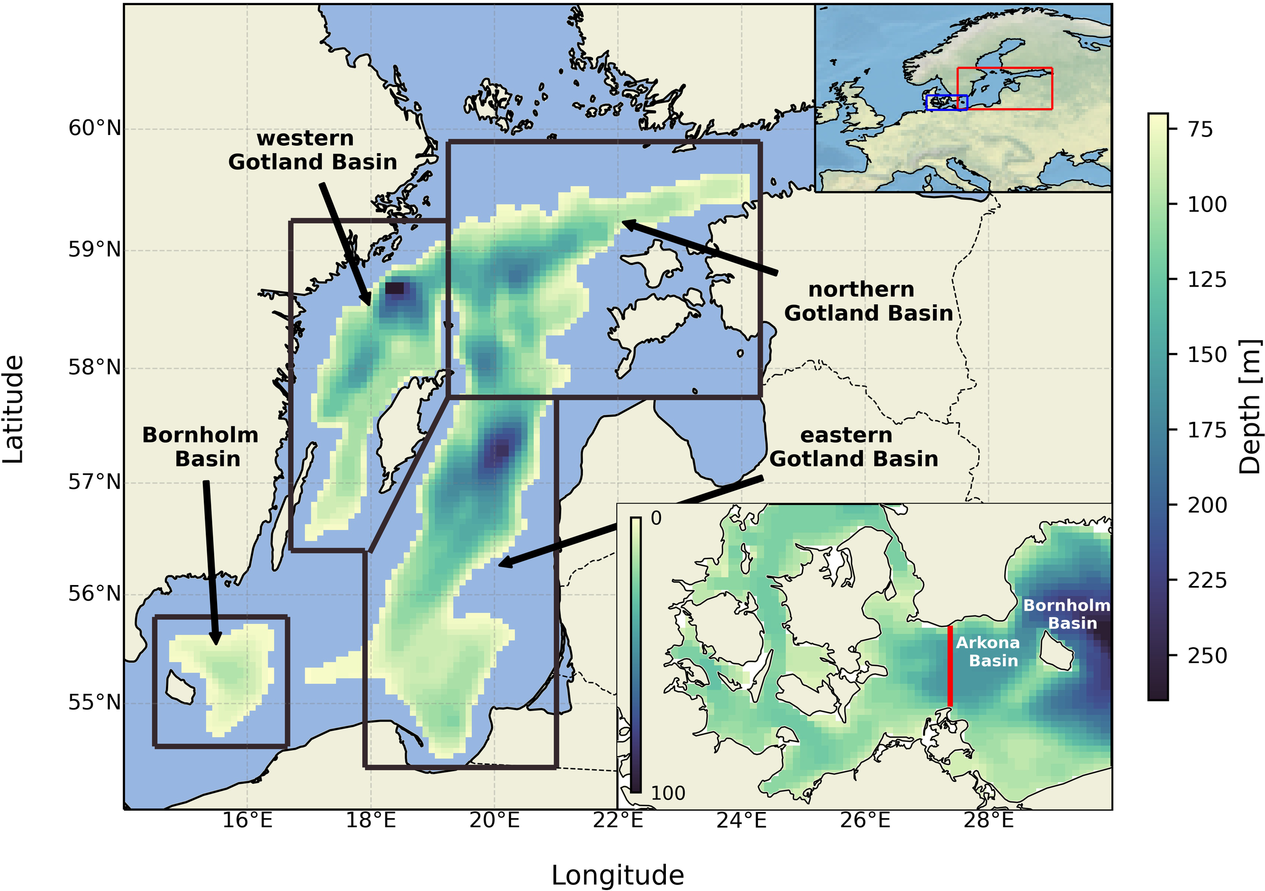
Model domain and boxes at 70 meters depth (boxes’ upper boundary). The transect used for inflow detection is shown in the lower right panel. The locations of the study area and the area from the lower right panel are shown on the upper right panel (red and blue boxes, respectively).
A natural ventilation mechanism for the central part of the Baltic Sea is provided by sporadic inflows of saline water through the Danish straits, so-called Major Baltic Inflow events (MBIs) (Matthäus and Franck, 1992; Matthäus et al., 2008; Hansson and Andersson, 2015; Lehmann et al., 2022). They occur under specific meteorological conditions and transport saline, oxygen-rich water from the North Sea into the Baltic Sea (Lehmann and Post, 2015; Mohrholz, 2018). Due to the high density, North Sea water flows along the bottom slope and fills the deep Baltic Sea basins (Bornholm Basin, Eastern, Northern, and Western Gotland basins) (see Figure 1), where the oxygen content is usually low. Neumann et al. (2017) compared two inflow events in 2003 and 2014, the latter being one of the strongest MBIs in the history of the observations. They concluded that the less intense 2003 event supplied more oxygen to the central Baltic Sea than the stronger 2014 event due to the longer overall duration of the consecutive inflow events which made out the 2003 event. However, this paper did not consider the possibly different biochemical responses to those two inflows. Another source of uncertainty is related to the biochemical response to the inflow’s oxygen-rich water. The study by Meier et al. (2018b) showed that oxygen consumption in the water column and the sediments has increased during recent decades, which can exceed the oxygen supply and even contribute to elevated hypoxia and anoxia.
Another mechanism controlling hypoxic area development in the Baltic Sea is the halocline depth and strength. This mechanism, which affects hypoxia via modulation of the vertical oxygen supply across the pycnocline, is controlled by small and mesoscale processes (Elken et al., 2006; Kuzmina et al., 2008; Conley et al., 2009; Väli et al., 2013). Increasing halocline strength (the salt gradient between upper and lower layers) limits the vertical exchange with the upper layer, which alleviates hypoxia. Strengthening of the halocline is known to accompany the Major Baltic Inflows (MBIs), potentially limiting their aeration effectiveness (Conley et al., 2002).
This study aims to address the oxygenation mechanisms of the central Baltic Sea by MBIs and its uncertainties with the help of a numerical model. This is done by investigating the 29 most significant oxygen inflows from 1948 to 2018 and their influence on oxygen and hydrogen sulfide sources and sinks in the deep water and sediments. Another goal is to disentangle oxygen and hydrogen sulfide sources and sinks in the central Baltic Sea to sort them for their contribution to the total oxygen variability on the interannual timescale, and to study their long-term trends.
2 Materials and methods
2.1 Model description
This study utilized a coupled hydrodynamical/biogeochemical 3-dimensional regional ocean model. A regional three nautical miles Baltic Sea setup of the Modular Ocean Model (MOM) (Pacanowski and Griffies, 2000; Griffies, 2004) served as a hydrodynamical model. This model uses a finite-difference method to solve the full set of primitive equations to calculate the motion of the water and the transport of heat and salt. K-profile parameterization (KPP, Large et al., 1994) was used as a turbulence closure scheme. The western open boundary was placed in the Skagerrak, enabling exchange with the North Sea. Model depths in the Baltic Sea setup, used in this study, were limited to 264 meters due to computational reasons related to the vertical grid representation. Hence, the Landsort Deep region was artificially shallowed. Potential uncertainties this approach entails are discussed in the Section 4. Biogeochemical cycles were simulated by the ERGOM model (Radtke et al., 2019; Neumann et al., 2021; Neumann et al., 2022). This model simulates the dynamics of the main nutrient elements, namely carbon (C), nitrogen (N), and phosphorus (P). Nitrogen and phosphorus are characterized by their organic and inorganic forms. ERGOM separates the phytoplankton community into three separate groups: large phytoplankton (lpp), small phytoplankton (spp), and cyanobacteria (cya). The zooplankton state variable (zoo) implements the grazing pressure on phytoplankton. There is a separate state variable representing detritus. Carbon is contained in these state variables in the fixed Redfield ratio and is additionally represented as particulate and dissolved organic carbon (DOC and POC), where the C:N:P ratio might be non-Redfield (Neumann et al., 2022), and dissolved inorganic carbon (DIC). ERGOM includes the closed O2 and H2S cycles, which can be briefly described as follows: oxygen is produced via the photosynthesis carried out by the phytoplankton and utilized in mineralization of organic matter and nitrification both in the sediments and in the water column. Hydrogen sulfide is represented as a separate state variable. It is produced under anoxic conditions via sulfate reduction and can be oxidized to sulfur, and subsequently to sulfate, either by oxygen or nitrates. The detailed description of all model equations can be found in Neumann et al. (2022). The model was forced by CoastDat2 meteorological forcing (Geyer, 2014) and time-dependent river runoff. The model setup used in this study has already been applied to the Baltic Sea and demonstrated a good performance in the study area (e.g. Neumann et al., 2017). The study’s time frame spanned the period from 1948 to 2018 (71 years). Two series of model results were produced. The first one was averaged monthly and the second one – daily. Monthly mean data were used in the budget analysis (Section 3.2) and daily mean – in the inflows’ ventilation analysis (Section 3.3).
2.2 Budget approach
Both physical and biochemical processes contribute to O2 budget in a particular volume in the sea. Physical terms of the oxygen budget include lateral and vertical advection and diffusion of oxygen into and out of the volume. Biochemical terms include mineralization of organic matter, photosynthesis, respiration of marine organisms, oxidation of reduced material (elemental sulfur, hydrogen sulfide, and ammonium), and denitrification. If the oxygen budget is positive, oxygen concentration increases within the considered volume, e.g., a selected box of a sub-domain, and vice versa. The same reasoning is applicable to H2S.
To perform the budget analysis, the central Baltic Sea was split into four boxes (see Figure 1). In the vertical, each box spans from 70 meters depth to the bottom. These boxes represent four different basins, namely the Bornholm Basin (BB) – the shallowest among all selected sub-basins with only the upper boundary active; the eastern Gotland Basin (eGB), which has two lateral boundaries: the Slupsk Furrow in the West, and the northern Gotland Basin in the North; and correspondingly the northern (nGB) and western (wGB) Gotland basins with two and one lateral boundaries, respectively. The fifth box, for which the analysis was conducted, represents the whole central Baltic Sea (the total area depicted in Figure 1) comprising all four boxes and the small Slupsk Furrow, westerly adjacent to the eGB. Mass conservation was checked for all boxes, both for oxygen and hydrogen sulfide. The errors are a few orders of magnitude less than all budget terms (see Supplementary Figures 1 and 2), which suggests that the coupled MOM-ERGOM model obeys the mass conservation law and can be utilized for this type of analysis.
2.3 Validation against the observations
The model setup was thoroughly validated against the observational and reanalysis datasets. Observational data are combined data sampled from the ICES (International Council of the Exploration of the Sea) web archive (ICES, 2023) and the IOW (Leibniz Institute for Baltic Sea Research Warnemuende) observational database (IOW, 2023). As another, continuous dataset for validation, the Copernicus regional Baltic Sea reanalysis (BALTICSEA_REANALYSIS_BIO_003_012) was chosen (Copernicus, 2023a). This product is based on the coupled NEMO/SCOBI model system (Almroth-Rosell et al., 2014; Hordoir et al., 2019) and includes data assimilation of oxygen concentration and nutrients observations (O2, P, N). It has two nautical miles horizontal resolution and 56 depth levels. Temperature and salinity fields were taken from the Copernicus regional physical reanalysis for the Baltic Sea (BALTICSEA_REANALYSIS_PHY_003_011) (Copernicus, 2023b). This reanalysis product is identical to the biological reanalysis. For simplification, later in the text and the figures, all fields from those products will be presented under the “Copernicus” label.
The evaluation was performed for several model variables (temperature, salinity, PO43-, NO3-, NH4+, O2 (dissolved oxygen), and H2S (dissolved hydrogen sulfide). Hypoxic area and volume, as the key indicators of redox conditions, were also validated against the Copernicus data. Only the climatological (1993-2018) oxygen profiles are shown in the paper (Figure 2). More validation results are presented in Supplementary Figures 5-17.
Figure 2
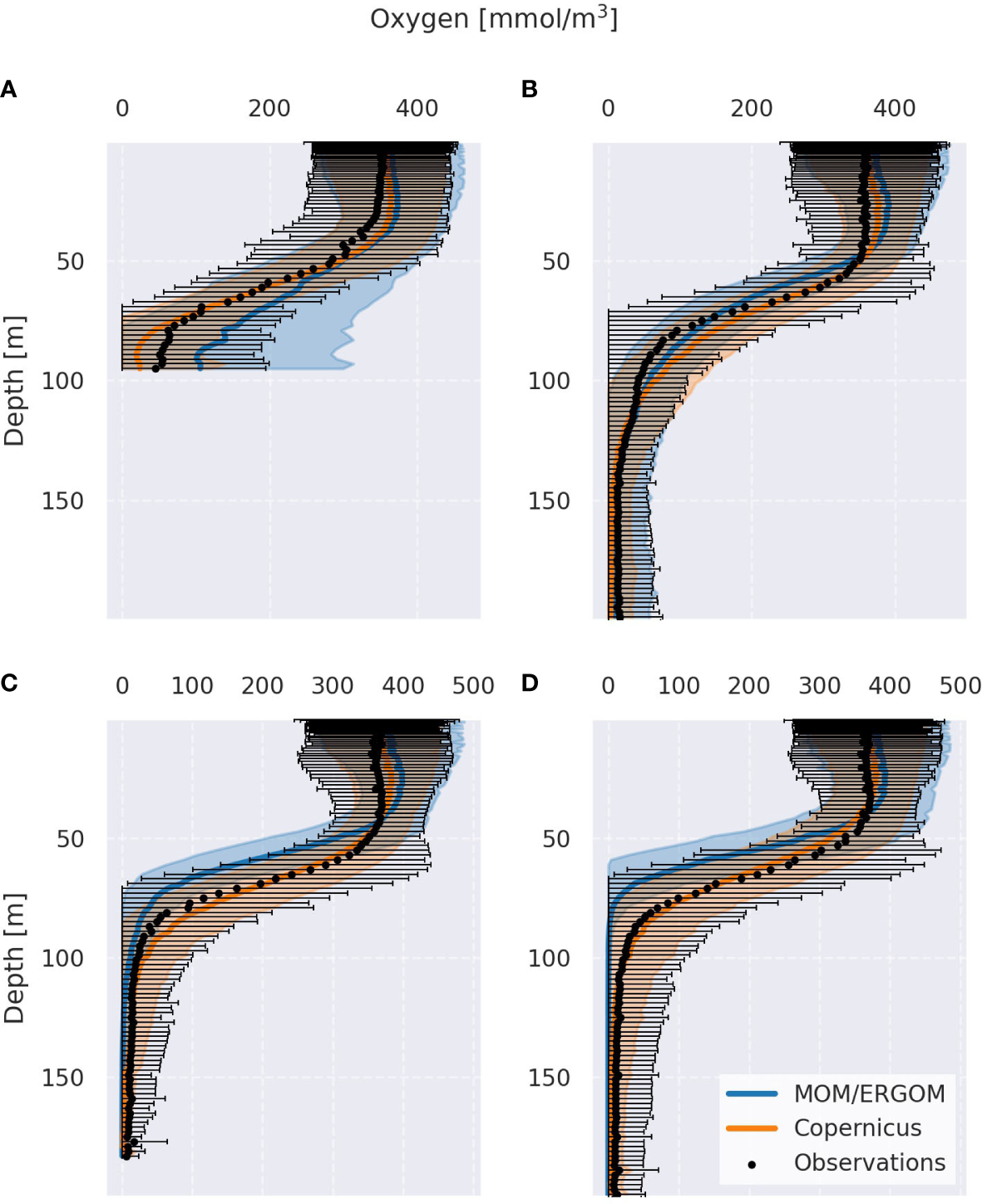
Climatological mean oxygen profiles (averaged from 1948 to 2018) for all sub-basins studied [Bornholm Basin (A), eastern Gotland Basin (B), northern Gotland Basin (C), and western Gotland Basin (D)]. Colored translucent and black hatched areas for model data and observations, respectively, show the variability (+- 2 s.d.).
2.4 Statistical methods used for sources and sinks processing
For the model data postprocessing, a few statistical methods were utilized. A simple linear regression model was applied to calculate the trends. Trend significance was checked by testing the statistical hypothesis about the equality of the trend slope coefficient to zero with α=0.05 employing the Wald test (Wald, 1943; Murtagh and Legendre, 2014). The linear regression framework has been adopted to rank the processes by the explained proportion of oxygen variance. Starting from a simple linear regression to the process that explains most of the variance, we then use a series of multilinear regressions, every time adding a single next process that increases the explained variance most. Relative contributions were calculated by comparing the two determination coefficients (R2) of neighboring fits.
A hierarchical agglomerative cluster analysis technique (Ward’s method) was chosen to classify the identified oxygen and saltwater inflows according to the import of oxygen/salt into the Baltic Sea (Ward, 1963). A distance matrix was computed using the Euclidean distance measure (Dokmanic et al., 2015) to get a classification based on the differences in the mean value. The cluster analysis aims to maximize the variance between the different clusters and minimize the variance within a single cluster. In agglomerative algorithms, all data points are attributed to the distinctive clusters at the first iteration, so the number of clusters equals the number of data points. In the next step, the closest clusters are merged, forming a bigger cluster. In the end, there is only one cluster encompassing all data points. The algorithm produces a diagram, so-called dendrogram, showing at which distance the specific clusters were merged. Dendrograms for total oxygen and salt transported into the Baltic Sea by inflows are shown in Supplementary Figures 18 and 19.
2.5 Inflows detection algorithm
Daily model total oxygen/salt transport across the vertical transect in the Arkona Basin (Arkona transect) (see Figure 1) was analyzed to detect the inflow events. The resulting time series was preprocessed with a 5-day running mean to remove the high-frequency variability. In the filtered time series, consecutive positive transport values for more than 5 days were considered to be an inflow event (Mohrholz, 2018). Supplementary Figure 20 shows the identified inflows for the year 1948. The statistics for oxygen and salinity inflows were collected from 1948 to 2018. They include the inflow’s start date, end date, duration, and the total amount of salt/oxygen transported during the event. Tables containing the 10 largest inflow events for oxygen and salt can be found in Supplementary Tables 3, 4. The hierarchical clusterization algorithm (described in the previous subsection) was applied to the total transport per inflow time series to classify the inflows by their strength. The oxygen transport time-series was split into four classes, while the salt transport time series was divided into two classes only (see Supplementary Figures 18, 19). Figure 3 demonstrates the main properties of identified O2 inflows clustered into four distinct clusters. The number of inflows per class varies significantly. There are 29 strong inflows, 147 moderate, 313 small, and 306 very small. Moderate and small inflows usually carry the most oxygen in years without strong inflows. In a year with strong inflows, these can constitute up to around 50% of the total oxygen transport by the inflows. Strong oxygen inflows are distributed unevenly on the time axis. There are periods with enhanced transport (the 1950s, 1972-1976, 1993-1994, and the 2010s) and periods with no transport (the 1960s, 1977-1992, 1999-2005). Overall, no trend was found, neither in the oxygen transport by the inflows, nor in the salt transport (for the salt inflows, see Supplementary Figure 21). Later we will only focus on the 29 strong oxygen inflow events. Although they might not constitute the largest oxygen source in a particular year, they all are accompanied by large salt inflows (according to the provided classification). This choice is essential because only inflows that reach the remote central Baltic Sea basins (eGB, nGB, and possibly wGB) shall be studied. To analyze all 29 strong inflows separately, the tagging method was applied following Ménesguen et al. (2006). That method allows having a separate tracer variable for oxygen brought to the Baltic Sea by a specific inflow event. The results are discussed in Section 3.3.
Figure 3
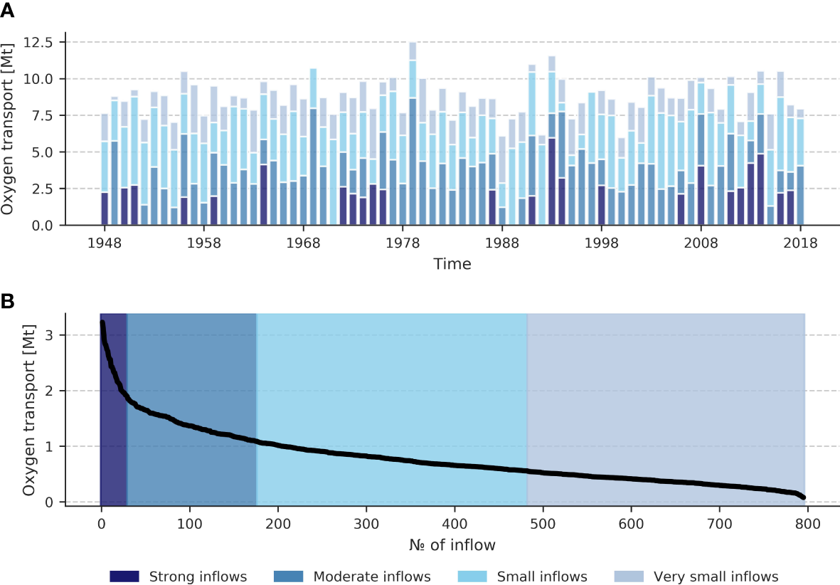
Total oxygen transport through the Arkona transect per year by each inflow class (A). Distribution of total oxygen transport per inflow sorted in descending order (B). Colors indicate inflow classes. The following classes were defined: strong inflows (carry more than 1.8 Mt O2), moderate inflows (carry from 1.8 Mt O2 to 1 Mt O2), small inflows (carry from 1 Mt O2 to 0.5 Mt O2), and very small inflows (carry less than 0.5 Mt O2). Mt stands for 109 kg.
3 Results
3.1 Validation summary
Validation showed that the coupled MOM/ERGOM model was able to reproduce the mean state and temporal variability of all investigated variables within each selected sub-basin (BB, eGB, nGB, and wGB). In Figure 2, model oxygen profiles are predominantly located within two standard deviations from Copernicus and observations. Validation also highlights some sources of uncertainty in the model estimates. Model overestimates hypoxic conditions in the whole Gotland Basin (especially in the wGB and nGB). At the same time, it underestimates hypoxia in the Bornholm Basin (see Supplementary Figure 5). This pattern can be seen in Figure 2 as well. Starting at 50 meters depth, the model oxygen profile in the BB positively deviates from both Copernicus reanalysis and observations. It also shows a weaker oxycline. Both in the wGB and nGB, model oxygen profiles demonstrate a stronger oxycline and an absence of variability below a certain depth (see Supplementary Figures 12, 14). The mechanisms that likely cause these oxygen misrepresentations are deviations in the halocline depth and strength in the MOM model (Supplementary Figure 17). Since there are no other significant deviations caused by ERGOM, the model results can be trusted, but the uncertainties should be considered.
3.2 Processes governing O2 and H2S dynamics in the central Baltic Sea
Understanding oxygen and hydrogen sulfide dynamics requires knowledge of the main processes governing their variability. In this Section, all processes contributing to the O2 and H2S budgets were analyzed in terms of average values and their temporal variability for each sub-basin.
3.2.1 The biggest O2 and H2S sources and sinks
First, we analyzed the time-averaged contributions to the oxygen and hydrogen sulfide budgets for each sub-basin. The processes were grouped into physical fluxes, water column processes, and sedimentary processes (see Supplementary Tables 1, 2).
For the oxygen budget, vertical advection dominates in the physical processes group in the BB, eGB, and wGB. In the nGB, lateral advection across the southern boundary brings the most oxygen into the domain. The other advection terms comparably contribute to oxygen supply to the eGB and wGB. However, this is less true for the nGB sub-basin, where both vertical and western advection terms are at least one order of magnitude less than the advective transport from the south. This pattern in oxygen advection indicates the importance of oxygen inflows for deep sea ventilation and separates sub-basins in terms of oxygen supply. BB and eGB are relatively close to the Danish straits and therefore receive more oxygen via the inflows. Conversely, wGB is a remote sub-basin with limited oxygen supply. Among the water column processes, nitrification was found to be the largest oxygen sink in all sub-basins except wGB, where oxidation of elemental sulfur turned out to be the biggest sink of oxygen. However, in the wGB, oxygen consumption by water column nitrification cannot be neglected. Elemental sulfur oxidation is one of the largest water column oxygen consumption terms in the eGB and nGB. Oxygen supply by photosynthesis and consumption by living organisms’ respiration is negligible in the whole study area. Oxygen consumption in the sediments is dominated by detritus mineralization, which is the biggest oxygen sink everywhere except wGB, where oxidation of elemental sulfur in the water column exceeds it. The contributions change over time, though. The biggest oxygen sink in the wGB changes from nitrification to sulfur mineralization. This, together with a decreased oxygen consumption in the sediments, could indicate a deterioration of oxygen conditions, where redoxcline movement to shallower depths facilitates the accumulation of reduced material in the sediments.
Sources and sinks of hydrogen sulfide differ from those of oxygen, their hierarchy is also different. Advection of hydrogen sulfide across the upper boundary out of the basin dominates among the advective and diffusive fluxes in the remote sub-basins (the nGB and wGB). In the eGB, the biggest advection term is the transport across the northern boundary, which brings H2S out of the domain towards the more remote basins, activating a positive feedback mechanism further worsening the oxygen conditions there. The water column serves mainly as a sink of hydrogen sulfide. Both H2S sink terms (oxidation by O2 and NO3-) contribute significantly to the hydrogen sulfide removal, having the same order of magnitude. Oxidation by O2 dominates in the BB and wGB, and oxidation by NO3-, - in the eGB and nGB. The biggest H2S production term in the water column is the mineralization of detritus. In the sediments, mineralization of detritus is also the biggest source of H2S across all sub-basins. Numbers are presented in Supplementary Tables 5-10.
3.2.2 Contribution of the different processes to the O2 and H2S variability
To study the dynamic aspect of O2 and H2S sources and sinks in the sub-basins, regression analysis (for the method description, see Section 2) was performed for both aggregated process categories (Figure 4) and individual processes (Supplementary Figures 22, 23). There are significant differences in oxygen and hydrogen sulfide dynamics. More than half of the oxygen’s variance is explained by physical processes. In contrast, hydrogen sulfide dynamics is governed by the water column processes, which explain 45% to 87% of its variability. The remaining groups do not have the same contributions from sub-basin to sub-basin. For oxygen, there is a slight increase in the explained variance by the water column processes in the remote sub-basins. At the same time, 17% of the variability in the wGB is explained by sedimentary consumption, which is the second largest fraction after 22% in BB. Analysis of the more specific processes’ contribution to the oxygen and hydrogen sulfide dynamics reinforces the conclusions about advection-driven oxygen dynamics. In all sub-basins, advective terms explain the largest fraction of variability. Coupled nitrification-denitrification processes in oxic sediments significantly contribute to the oxygen variability in the BB and eGB. However, in the nGB and wGB, those processes are not included in the list of significant processes, giving their place to nitrification in the water column. In the nGB, the only considerable process related to the oxygen consumption in the sediments is mineralization of the particulate organic matter (POM) (including both detritus mineralization and mineralization of non-Redfield particulate organic carbon (POC)). In the wGB, no critical processes related to sedimentary consumption are detected.
Figure 4
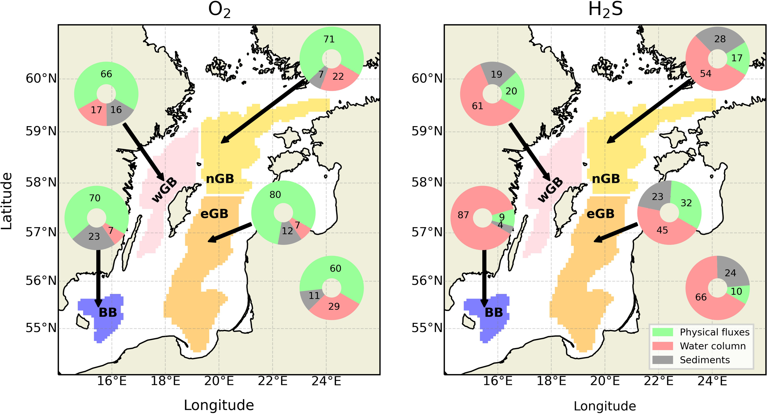
Fraction of interannual O2 (left panel) and H2S (right panel) variability (in %) explained by the certain group of processes, namely physical fluxes, which includes advection, diffusion, and other physical processes, water column, which includes all processes from O2 or H2S budgets situated in the water column, and sediments, which includes all processes situated in the sediments. The numbers are presented inside the pie-charts. Different sub-basins are marked by areas with different colors. The lower right pie-charts represents the whole central Baltic Sea. See Supplementary Tables 1 and 2 for more information about processes in each category.
Analysis of terms contributing to hydrogen sulfide dynamics featured some notable patterns. Oxidation, either by O2 or NO3-, explains the significant fraction of H2S variability everywhere in the central Baltic Sea. Among the sedimentary processes, the mineralization of detritus is the universal significant term in all sub-basins. This clearly distinguishes water column and sediments, making former the sink of H2S and latter - the source. Both lateral and vertical advection terms play an important role in the hydrogen sulfide dynamics only in the two remote basins. This again stresses their vulnerable position as H2S producers and, in addition, sinks of hydrogen sulfide from the neighboring basins.
3.2.3 Temporal variability of O2 and H2S sources and sinks
A linear trend analysis has been conducted to detect shifts in oxygen and hydrogen sulfide budget terms (Figures 5, 6). No significant change in oxygen supply by the physical fluxes was found anywhere except in the BB (Figure 5A). That trend might be attributed to internal changes within the basin, e.g., stratification or unidentified small inflows. Trends in the oxygen consumption in the water column and sediments are not identical from region to region. In the BB, both water column and sedimentary consumption exhibit a significant negative trend (i.e., an increase in their magnitude, since consumption is counted negative). Other sub-basins show the common pattern of temporal variability in the water column and sedimentary oxygen consumption. It is a significant negative trend in water column consumption [found in the eGB (Figure 5B) and nGB (Figure 5C)], and a significant positive trend in the sedimentary consumption [found in the nGB and wGB (Figure 5D)], which represents a shift in oxygen consumption from sediments to the water column. The most pronounced example of that pattern is the nGB, where initially consumption in the sediments dominated over consumption in the water column but, starting from the 1980s, the latter exceeds the former, highlighting the shift of oxygen consumption from the sediments to the water column. No significant trend in the water column consumption was observed in the wGB, but there is a significant, positive trend in the sedimentary consumption. This could indicate that the worsening of oxygen conditions across the remote basins in the central Baltic Sea is started in the 1970s and is still happening. It is especially visible in the wGB, where the absence of a negative trend in the water column consumption indicates elevated import of reduced material, including H2S.
Figure 5
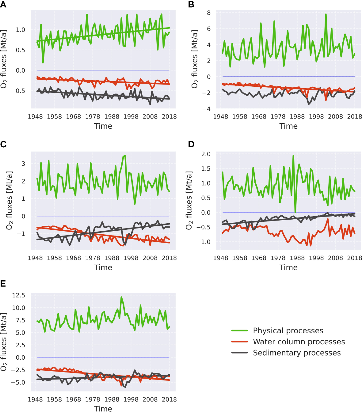
Linear trends of groups of processes governing oxygen dynamics in the sub-basins, namely the Bornholm Basin (A), the eastern Gotland Basin (B), the northern Gotland Basin (C), the western Gotland Basin (D), and the whole central Baltic Sea (E). The groups of processes are identical to those in Figure 4. Trend lines are only shown if they are significant (p<0.05). Mt/a stands for 109 kg per year. See Supplementary Table 1 for more information about processes in each category.
Figure 6
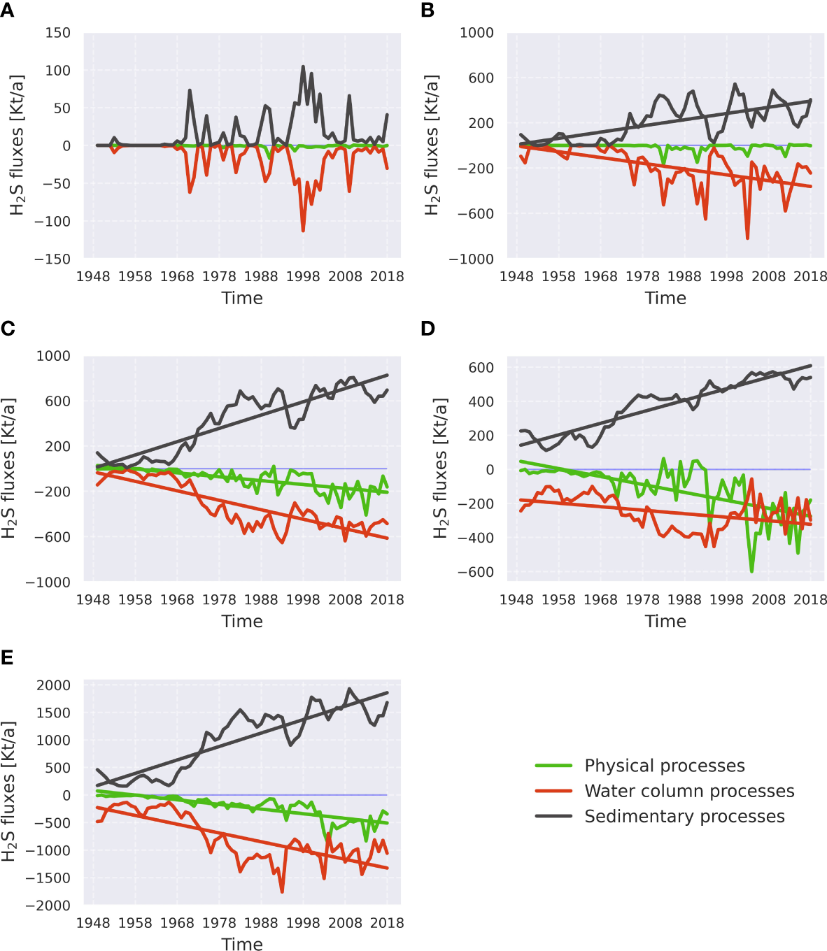
As Figure 5 but for hydrogen sulfide. The order of subplots is the same as in Figure 5: (A) - the Bornholm Basin, (B) - the eastern Gotland Basin, (C) - the northern Gotland Basin, (D) - the western Gotland Basin, and (E) - the whole central Baltic Sea. Kt/a stands for 106 kg per year. See Supplementary Table 2 for more information about processes in each category.
Trends of the H2S production/consumption exhibit some spatial variability. In the BB diagram (Figure 6A), the curve, indicating H2S consumption in the water column, is mirrored by the H2S sedimentary production curve without any significant linear trend. This pattern reflects the fact that there is no long-term accumulation of hydrogen sulfide happening in the BB. All H2S produced here is oxidized within a short time. H2S terms across the different regions of the Gotland Basin exhibit the significant linear trends in water column consumption and sedimentary production with the opposite signs. No significant trend in physical fluxes was found in the eGB (Figure 6B), whereas in both nGB (Figure 6C) and wGB (Figure 6D), a significant negative trend in physical processes was observed, meaning the export of H2S out of the sub-basin. The magnitude of the trend in physical fluxes follows the difference between magnitudes of the water column H2S consumption and sedimentary H2S production trends. See Supplementary Tables 11, 12 for information about the trends of individual processes.
3.3 Ventilation by inflows
As shown in the previous section, advection governs the oxygen dynamics in the deep basins of the central Baltic Sea. The sole mechanism of oxygen advection into the deep waters is the Baltic Sea inflows, transporting oxygen and salt from the North Sea through the shallow and narrow Danish straits. In this section, the dynamics of oxygen inflows have been rigorously assessed. Despite the constant exchange between the Baltic Sea and the North Sea via small and medium-sized inflows, the biggest inflows are of primary importance for the ventilation of the deepest parts of the central Baltic Sea. We utilized the approach proposed by Ménesguen et al. (2006) to tag the oxygen that enters the Baltic Sea with the 29 biggest inflows that happened from 1948 to 2018 and were identified in advance (see Figure 3 and Section 2.5 for more details). The tagging was activated in total 29 times (each time when inflow water arrives at the Arkona transect depicted in Figure 1). We tagged all dissolved oxygen below 70 meters depth west of the Arkona transect. The tagging was stopped at the end of the inflow event (this means no new tagged oxygen is generated, however, the old one remains). This approach allowed us to track oxygen brought to the Baltic Sea by a specific inflow event. The tagged oxygen is modeled as an additional active biogeochemical tracer, which participates in its own set of reactions and undergoes separate advection and mixing. In total, 29 additional tracers were added to the model, each one representing a certain inflow event. The described tagging approach was also employed in Neumann (2007); Radtke et al. (2012), and Neumann et al. (2017).
3.3.1 Temporal trends in inflows’ ventilation
To study the temporal patterns of the ventilation by saltwater inflows, analysis of the regional inflowed oxygen content and inflows’ lifetime was conducted. (Figure 7A) revealed no presence of a significant trend in the inflows’ strength, this statement is supported by Figure 3. At the same time, a clear negative trend is visible in the inflows’ lifetimes across all sub-basins (Figure 7, right panels). All linear trends explain more than 30% of the variability, with the lowest numbers in the BB and the highest in the wGB. This sub-basin also demonstrates the steepest trend across all four sub-basins. The inflow-derived oxygen content in the wGB (Figure 8H), which is generally very limited in the wGB, also shows a rapid decline. The inflows after 1965-66 brought almost no oxygen. Even the largest inflows, which happened in 1993-94 and 2014-15, brought nearly no oxygen to the wGB. The nGB exhibits, in general, the same behavior as the wGB. The largest inflows, which took place in the 1990s and the 2000s, brought less oxygen to the sub-basin than inflows from the 1960s. This might be attributed to the elevated oxygen consumption in the nGB and in other sub-basins. In the BB and eGB, no significant decrease in the inflow-derived oxygen content was found. In the BB, the large fraction of oxygen is usually originating from the inflows. In the eGB, this number drops two times. The most considerable amount of oxygen was brought to the BB and eGB during the 1993-94 inflows. Considering the results presented in Figure 7, it can be concluded that currently all four sub-basins are less well oxygenated by saltwater inflows than 70 years ago. This is especially visible in the remote nGB and wGB, where the total content of inflowing O2 dramatically dropped compared to the first half of the 20th century. Assuming no significant trend in the inflows’ strength (amount of O2 transported across the Arkona transect), the only reason for those changes is accelerated oxygen consumption provoked by the overall deoxygenation of the central Baltic Sea.
Figure 7
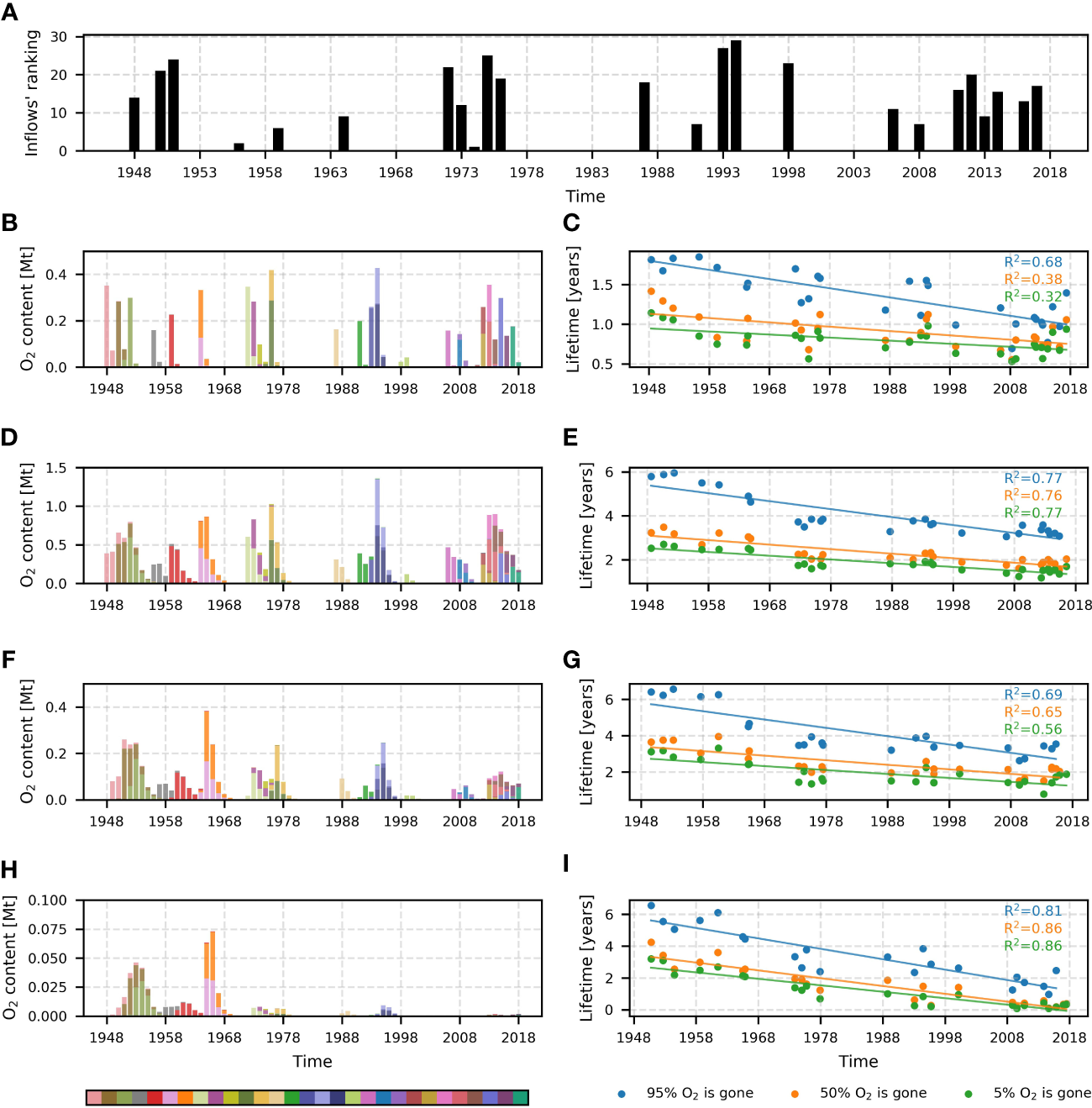
Ranking of inflows based on the total amount of oxygen transported across the Arkona transect during the inflow event panel (A). Number 29 stands for the inflow that transported the most oxygen, and number 1 for one that transported the least oxygen. The total yearly content of oxygen transported by saltwater inflows to different sub-basins is depicted in panels (B, D, F, H). Different inflows are shown as different colors in the histogram. Bar heights represent the inflow’s O2 content in a certain sub-basin. The color bar shows the colors of inflows in chronological order (the earliest inflow is pink, the next one is brown, etc.). Panels (C, E, G, I) show the lifetime of inflow oxygen for each sub-basin (dots). Lifetime is defined as the time when inflow oxygen reaches a certain fraction of its maximal value. Three fractions are shown: 5% of inflow O2 is consumed (95% remaining) - green dots, 50% of inflow O2 is consumed (50% remaining) - orange dots, 95% of inflow O2 is consumed (5% remaining) - blue dots. Linear trends, demonstrating the decay of inflowing O2 lifetime, are shown for each scatter plot. Determination coefficients (R2) for each linear trend are presented in the upper-left part of the panels. Their colors indicate the trends they belong to. Panels (B, C) stand for Bornholm Basin, (D, E) – for eastern Gotland Basin, (F, G) – for the northern Gotland Basin, H and I – for the western Gotland Basin. Mt corresponds to 109 kg.
Figure 8
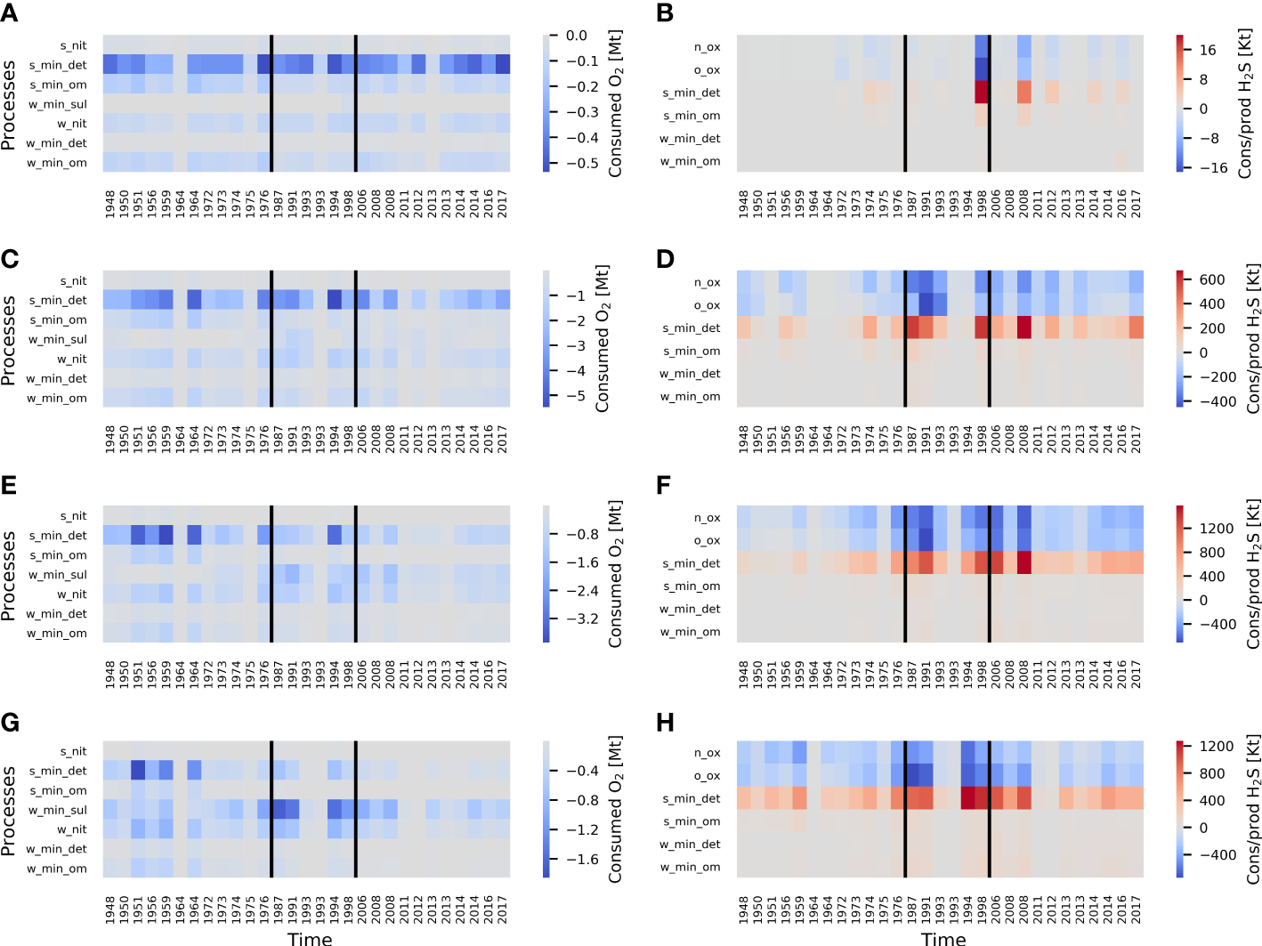
Temporally integrated oxygen consumption (negative values) panels (A, C, E, G) and hydrogen sulfide consumption (negative values) and production (positive values) panels (B, D, F, H) by a specific term during saltwater inflows for each sub-basin (spatially integrated within the sub-basin). Integration was carried out for the total daily consumption or production by a certain budget term. For each sub-basin integration started when a certain inflow reached that sub-basin and stopped when either all O2 transported by the inflow is consumed or the water of the new inflow reached the sub-basin. Processes should be read according to the following rule: the first part of the name shows the domain (w – water column and s -sediments), second and third parts – the type of process. For example, S_min_det should be read as detritus mineralization in the sediments. Respiration by phytoplankton and zooplankton as well as photosynthesis were excluded from the analysis due to their pronounced seasonality and their unimportance for the oxygen budget (see Section 3.1). X-axis shows the years when the inflows begin and therefore is not equally spaced but sticks to the chronological order. Black lines denote stagnation periods. Panels (A, B) stand for the Bornholm Basin, (C, D) – for the eastern Gotland Basin, (E, F) – for the northern Gotland Basin, (G, H) – for the western Gotland Basin. Mt corresponds to 109 kg. Kt corresponds to 106 kg. See Supplementary Tables 1, 2 for the definition of the names of processes.
3.3.2 Changes in ventilation pattern
It has been shown that there is a significant decline in inflowing oxygen lifetime in the deep waters (below 70 m) across the central Baltic Sea, especially the nGB and wGB. However, we did not yet investigate which processes contributed most to the enhanced inflowing oxygen consumption and whether the pattern of inflowed O2 consumption is changing with time. To answer that question, temporally integrated oxygen consumption and hydrogen sulfide production/consumption per process (or per group of processes) was calculated for each of the inflows (for more details, see Figure 9). The integration for a specific inflow is stopped when (a) another inflow event occurs or (b) the oxygenation by the inflow has ended. From the analysis of Figure 9, it can be noted that mineralization of detritus is the process consuming most oxygen in all sub-basins. However, in the remote nGB and wGB, water column processes play a larger role, namely the oxidation of sulfur and H2S (the sum of two processes, namely, oxidation of H2S to elemental S and oxidation of elemental S to SO42-) and nitrification. It fits the conclusions about shifting the main oxygen sink from sediments to the water column demonstrated in the previous sections.
Figure 9
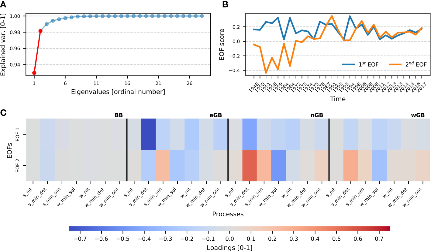
Results of the EOF analysis for oxygen consumption during inflow events. Panel (A) demonstrates the fraction of variance explained by the EOFs. The first two EOFs (which explain more than 95% of the variance) are marked by red color. Only those two EOFs were considered. Panel (B) shows timeseries of the first two EOFs. Note that the x-axis in panel A is not equidistant (see caption of Figure 8). The first EOF exhibits a stationary pattern, whereas the second demonstrates some non-stationarity. Panel (C) shows the EOF loadings, which indicate how a certain EOF is connected to a certain process. Positive values (red) indicate a direct relationship between EOF and a process, negative (blue) - a reverse relationship. It is visible that the first EOF shows reverse relationships with all processes, but the second shows both types of relationship. Processes are read the same way as in Figure 8, but with the ending indicating a certain sub-basin. The processes in the matrix are sorted in the following way: the Bornholm Basin, the eastern Gotland Basin, the northern Gotland Basin, and the western Gotland Basin. Black vertical lines denote the boundaries between sub-basins. See Supplementary Table 1 for the definition of the names of processes.
For the hydrogen sulfide budget, the most important source during the inflow events is the mineralization of detritus in the sediments. Sinks of H2S are oxidation by O2 and NO3-, which similarly contribute to the H2S consumption. No time-dependent pattern of H2S consumption and production is observed in the wGB. In the nGB and eGB, the slight increase in both production and consumption of H2S starting from the 1970s is visible.
To identify and understand the dominating patterns in the O2 and H2S dynamics during the inflow events, EOF analysis (Hannachi et al., 2007) was conducted for these spatiotemporal matrices. The results (see Figure 8) suggest that there are two EOFs describing more than 95% of the variance in O2 data. The first EOF explains approximately 90% of the variability, and the second explains about 5% (Figure 8A). Loadings of the first EOF demonstrate no spatial dependency, having the same sign across all sub-basins. The first spatial pattern thus describes a default reaction of all basins to an inflow that brings oxygen, while the first EOF varies with the amount of oxygen input and is positively correlated with the duration of the inflow effect (Figure 8C). The first EOF might be attributed to the inflow’s strength and duration because those patterns are spatially independent and should affect especially eGB since it is the first deep basin on the way of the inflowing water. The second EOF shows more sophisticated dynamics. It changes in the sign during the 1970s indicating the shift in contributing processes (Figure 8B). Loadings of the second EOF show opposite patterns between the sub-basins, which indicates the spatial non-uniformness of the pattern behind the second EOF. What the second EOF reveals is a change in the oxygen-consuming processes between the two periods before and after the 1970s. This change in the processes is opposite between the basins. A strong inflow in the later period differs from a strong inflow in the earlier period by a larger value of the second EOF. That means that the corresponding loads (lower panel of Figure 8) directly show the change in the reaction of the basins to an oxygen input. Since all processes in the figure are consuming oxygen, the negative values (shown in blue) mean an amplification. Oxygen consumption for the mineralization of sedimentary detritus is shifted spatially. It is enhanced in the eastern Gotland Basin and reduced in the northern and western Gotland Basin. An increase in all subbasins is seen for the consumption related to sulfur oxidation (w_min_sul), but it is most pronounced in the nGB.
The EOFs for the H2S budget (Supplementary Figure 27) show approximately the same pattern, a positive but fluctuating EOF1 and an EOF2 that is slightly increasing. So, we can interpret the spatial pattern of the second EOF in the same way, as a change in the reaction of the Baltic Sea to inflowing oxygen. The production of H2S in the sediments shifts from the remote wGB to the nGB and the eGB located upstream of the inflow plume. Also, its consumption by oxidation is shifted upstream, but to a lesser extent, which means that the downstream transport of H2S increases.
The EOF analysis thus essentially confirms the previous findings showing that just these two patterns, (a) a constant spatial signal that varies with the amount of imported oxygen and (b) the change in processes explain more than 95% of the variance. The spatial redistribution described by the second EOF can almost completely explain the spatiotemporal variability seen in the model, with the first EOF explaining the overwhelming part of the variability. So, it could be stated that inflows’ duration and strength govern the oxygen consumption with some little variability explained by the shifted consumption due to the overall deoxygenation.
4 Discussion
The Baltic Sea is experiencing deteriorating oxygen conditions in the deep waters despite the adopted nutrient loads reduction policy (Carstensen and Conley, 2019; HELCOM, 2021; Krapf et al., 2022). The reason for that might be related to the slow system response to the changing forcing (Gustafsson et al., 2012) and the “vicious circle” of eutrophication (Vahtera et al., 2007). This research indicates, based on a model experiment, significant deterioration of oxygen conditions across the central Baltic Sea, which includes significant negative long-term trends of oxygen concentration and positive long-term trends of the concentration of the reduced material (ammonium and hydrogen sulfide). This is clearly shown in Figure 10 (right panels). Rolff et al. (2022) studied the oxygen debt (the amount of oxygen required to oxidize all reduced material) and its dynamics based on observational data. They found a significant contribution by NH4+ to the oxygen debt, as well as the oxygen debt’s increase, especially in the remote basins. Our results are well-aligned with the results by Rolff et al. (2022). As was shown, the mineralization of detritus in the sediments acts as the biggest oxygen sink across all sub-basins. Ammonium is produced as a product of detritus mineralization. Since detritus mineralization is increasing, so is ammonium release. This process explains positive trends in NH4+ in the deep waters of the central Baltic Sea and accelerates further oxygen consumption (which is supported by the high oxygen consumption by nitrification observed in the model).
Figure 10
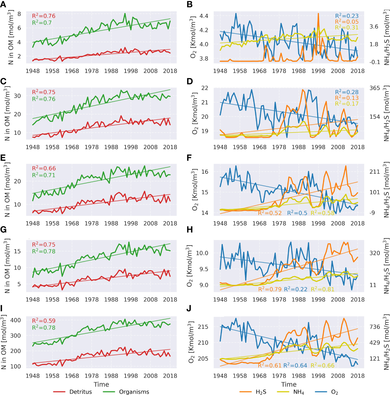
Linear trends of some important variables actively participating in oxygen and hydrogen sulfide dynamics. Left panels depict detritus concentration and concentration of living organisms (phytoplankton and zooplankton) integrated over the whole water column and all sub-basins: the Bornholm Basin (A, B), the eastern Gotland Basin (C, D), the northern Gotland Basin (E, F), the western Gotland Basin (G, H), and the whole central Baltic Sea (I, J). All variables are represented by nitrogen in organic matter (N in OM). Right panels show the dynamics of oxygen, hydrogen sulfide, and ammonium. Only significant linear trends (p<0.05) are shown.
The observed trends in oxygen consumption in the model were attributed to the worsening of oxygen conditions across the central Baltic Sea and uplifting of the redoxcline. The bacterial communities living in the suboxic and sulfidic waters are quite different (Hannig et al., 2006; Anderson et al., 2012). Discussed changes in the central Baltic Sea, especially in the Gotland Basin, should be visible in the long-term observational data related to the bacterial communities. A trend analysis in bacterial abundances, like Hoppe et al. (2013) did for the near-coastal site of Boknis Eck, could be used to verify (or falsify) the modelled trends.
The reason behind elevated trends in phytoplankton and detritus concentrations is not completely clear. The hypothesis about an extended vicious circle proposed by Meier et al. (2018b) is credible. However, we propose an additional positive feedback mechanism: NH4 emerging after detritus mineralization might be advected to the upper layer and thereafter might accelerate further phytoplankton growth. Meier et al. (2018b) conducted a model experiment studying oxygen sinks from 1850 to 2015. They found a shift toward the water column oxygen consumption. Our study supports this result. In addition, our method allowed the detailed analysis of various sub-basins. It was shown that the most notable change happened in the nGB, where initially, the sediments consumed more oxygen, but today, the water column took the role of the dominant oxygen sink. The same pattern, but not as pronounced, was observed in the eGB and wGB. Meier et al. (2018b) also observed drastically increased water column respiration by phytoplankton and higher trophic levels as well as nitrification, making them the dominant oxygen sinks during the last decade of their simulation. In our study, an increase in phytoplankton and zooplankton biomasses was also found (see Figure 10, left panels) as well as the increasing nitrification. However, no significant role of biota respiration was found. The possible source of disagreement might be related to different process formulations in the different models (RCO-SCOBI and MOM-ERGOM), specifically the zooplankton respiration, which can be used as a closure term representing the effect of higher trophic levels that are not represented in the model.
The 29 biggest oxygen inflows from 1948 to 2018 were studied separately, using the element marking approach proposed by Ménesguen et al. (2006). Most oxygen was brought to the deep central Baltic Sea during the 1993-1994 inflow events. Although, in accordance with Mohrholz (2018), no trend in the inflow activity was found, and the change of ventilation pattern related to the oxic state of the deep waters shows little variability, significant negative trends of inflow oxygen lifetime were observed everywhere, especially in the nGB and wGB. Therefore, the strongest inflow 2014-2015 did not ventilate deep waters so well not only due to the shorter duration compared to the 1993-1994 event, but also because of more elevated reducing conditions, especially in the nGB and wGB.
The model uncertainties, presented in Section 2, are likely related to the overestimation of halocline strength, which in turn is related to the overestimated salt transport from the North Sea due to the model resolution. The biggest misrepresentation was observed in the Gulf of Finland and the Bothnian Sea, both of them were excluded from the analysis. However, their effect on the closest nGB was not quantified. Considering the circulation of the deep water in the Baltic Sea, the transport is mainly directed towards the Gulf of Finland and the Bothnian Sea (Elken and Matthäus, 2008). The reversed transport is mainly carried out in the upper layer, so the overestimation of the Gulf of Finland’s and the Bothnian Sea’s hypoxia should not affect the nGB significantly. Another possible uncertainty, related to the artificially shallowed Landsort Deep, is negligible due to the very small affected area (0.19 km2, which corresponds to roughly 1% of the total wGB area, which is 17.62 km2). Deepening the Landsort Deep won’t change the composition of the processes either since even the shallowed Landsort Deep is constantly anoxic in our model. The more considerable uncertainties are related to representation of the biological community by ERGOM. In ERGOM, the full spectrum of phytoplankton species is divided into three functional groups. This assumption does not represent the changing Baltic Sea phytoplankton community (Olli et al., 2011). However, Wasmund et al. (2011) and Suikkanen et al. (2007) found long-term trends in some phytoplankton species based on observational data, proving at least the tendency of increasing phytoplankton concentrations in ERGOM. In addition, in other model studies the increase in phytoplankton biomass, primarily related to the availability of nutrients, is shown (Hieronymus et al., 2018). Also, the absence of refractory detritus in the ERGOM model may lead to exaggeration of the detritus mineralization, which might possibly contribute to the results. In addition to the refractory matter that is completely preserved, organic matter in the sediments can be remineralized at very different rates depending on its composition, which will strongly influence the time scales on which the sedimentary carbon pool influences the oxygen budgets. What is also missing in the model is a representation of iron and manganese, which take part in the redox cycle (Henkel et al., 2019; Schulz-Vogt et al., 2019). In reality, oxidation of H2S or organic matter may happen implicitly, by reducing iron or manganese oxides and later on oxidizing the reduced metals again by oxygen. Uncertainty is introduced here since these metals also have sources (e.g. from riverine input) and sinks (e.g. for iron in the form of pyrite).
All the discussed uncertainties make it very difficult to build a robust comparison between modeled processes and the actual ones. Here, we only present qualitative estimates. Hietanen et al. (2012) studied nitrogen-related processes situated at the oxic-anoxic interface in the Baltic proper. They found an increased rate of nitrification at the oxic-anoxic interface, which was also in general observed in our model results. Schneider and Otto (2019) calculated mineralization rates in the deep layer. Although we could not directly compare our results, we also observed some similar patterns, e.g., acceleration after the inflow. However, we were able to validate the vertical oxygen transport in the eGB with the observational data from Holtermann et al. (2022). According to their measurements, the mean annual vertical oxygen flux in the eGB equals to 2.39-3.97 Mt O2 year-1. Our results suggest a mean flux of 3.75 Mt O2 year-1, which aligns with their results. However, this comparison might be misleading due to the different definition of the eGB’s areas, different depths (our fluxes are calculated across the 70 meters depth layer, not across the pycnocline), and different study periods.
The obtained results shed light on long-term dynamics of processes related to the O2 and H2S budgets in the central Baltic Sea, which is not possible to capture via the observations due to irregular measurement campaigns and the complexity of the data postprocessing. Although model (Eilola et al., 2011; Meier et al., 2018b; Savchuk, 2018) and observational (Schneider et al., 2002; Gustafsson and Stigebrandt, 2007; Schneider et al., 2010; Schneider and Otto, 2019) studies, as well as studies related to the inflows’ propagation (Liblik et al., 2018), have already been conducted, this study covers wide spatial and temporal scales and decomposes O2 and H2S budget terms based on their contribution to their variability. The results suggested that a better trophic state for the future Baltic Sea is still beyond the grasp.
5 Conclusions
The employed analysis allowed us to sort the processes, contributing to the O2 and H2S budgets, according to their importance for the overall dynamics of those elements. It was found that the inter-annual oxygen dynamics is mainly governed by advection in all sub-basins, whereas hydrogen sulfide is mainly driven by local production and consumption. Mineralization of detritus in the sediments and nitrification are found to be the biggest oxygen sinks. These processes are coupled with each other because ammonium is the result of the oxidation of detritus, so the oxygen debt generated by detritus is resolved in two steps: mineralization of detritus itself and nitrification later. Mineralization of detritus is also the biggest producer of hydrogen sulfide in the sediments in the whole central Baltic Sea. The water column acts as the sink of H2S, where the oxidation both by NO3 and O2 contribute equally to the H2S consumption.
Analysis of the linear trends in the three categories of processes contributing to the O2 and H2S budgets (water column processes, physical fluxes, and sedimentary processes) revealed different regional dynamics. Amplified oxygen consumption in the water column and the sediment was observed in the Bornholm Basin with the latter dominating. A different pattern was observed in the three Gotland basins that showed a shift to dominating water column consumption. The overall transition from sedimentary to water column oxygen consumption was connected to the shortage of oxygen in the sediments which resulted in the upward movement of the redoxcline. An amplified upward spread of H2S in the wGB and nGB was found as a result of its deposition there.
We found a dramatic decrease in the content of O2 from inflows in the nGB and wGB that started in the second half of the 20th century. As no significant trend in inflow strength was found, the decreased lifetime is attributed to the amplified oxygen consumption, which was also observed.
Two significant EOFs of oxygen consumption after inflows per sub-basin were identified with the first EOF explaining more than 90% of the variability and the second explaining approximately 5%. The first EOF showed no spatial dependence and was attributed to the inflow duration and strength. The second EOF describes the response to the deoxygenation of the central Baltic Sea. It leads to the shift of the inflowing O2 consumption from the mineralization of detritus to the oxidation of H2S and elemental sulfur in the nGB and wGB. However, since the overwhelming fraction of variability is explained by the first EOF, we conclude that the duration and strength of inflows are the key parameters determining ventilation regardless of the trophic state of the sea.
Statements
Data availability statement
Reanalysis and observational data used in this study can be found under Copernicus, ICES, and IOW webpages (https://data.marine.copernicus.eu/products, https://www.ices.dk/data/dataset-collections, and https://odin2.io-warnemuende.de, respectively). The data, which are needed to reproduce the analysis shown in the study, are stored on Zenodo (https://doi.org/10.5281/zenodo.7661035). The full monthly-mean generated model data are stored on the IOW server (http://doi.io-warnemuende.de/10.12754/data-2023-0003).
Author contributions
LN, HR, and TN set up the model simulation with additional tracers. LN, with the help of TN, performed the budget analysis. LN, with the help of HR, performed the statistical analysis of the model data. LN validated the model data against observations and reanalysis dataset and wrote the manuscript with the help of all co-authors. HM and LN designed the research. HM supervised the work. All authors contributed to the article and approved the submitted version.
Acknowledgments
The research presented in this study is part of the Baltic Earth program (Earth System Science for the Baltic Sea region, see http://www.baltic.earth). The model simulations were performed on the computers of the North German Supercomputing Alliance (HLRN). The long-term observation program of the IOW is partly financed by the Bundesministerum für Verkehr und digitale Infrastruktur (BMVI) and is a part of the Baltic Monitoring Program (COMBINE) of HELCOM. Some observational data were taken from ICES database. Additionally, we would like to thank the two reviewers for their constructive and helpful comments, which facilitated the improvement of the manuscript.
Conflict of interest
The authors declare that the research was conducted in the absence of any commercial or financial relationships that could be construed as a potential conflict of interest.
Publisher’s note
All claims expressed in this article are solely those of the authors and do not necessarily represent those of their affiliated organizations, or those of the publisher, the editors and the reviewers. Any product that may be evaluated in this article, or claim that may be made by its manufacturer, is not guaranteed or endorsed by the publisher.
Supplementary material
The Supplementary Material for this article can be found online at: https://www.frontiersin.org/articles/10.3389/fmars.2023.1175643/full#supplementary-material
References
1
Almroth-Rosell E. Eilola K. Kuznetsov I. Hall P. Meier M. (2014). A new approach to model oxygen dependent benthic phosphate fluxes in the Baltic Sea. J. Mar. Syst.144, 127–141. doi: 10.1016/j.jmarsys.2014.11.007
2
Almroth-Rosell E. Wåhlström I. Hansson M. Väli G. Eilola K. Andersson P. et al . (2021). A regime shift toward a more anoxic environment in a eutrophic Sea in northern Europe. Front. Mar. Sci.8. doi: 10.3389/fmars.2021.799936
3
Anderson R. Winter C. Jürgens K. (2012). Protist grazing and viral lysis as prokaryotic mortality factors at Baltic Sea oxic–anoxic interfaces. Mar. Ecol. Prog. Ser.467, 1–14. doi: 10.3354/meps10001
4
Belkin I. M. (2009). Rapid warming of Large marine ecosystems. Prog. Oceanogr.81, 207–213. doi: 10.1016/j.pocean.2009.04.011
5
Breitburg D. Levin L. A. Oschlies A. Grégoire M. Chavez F. P. Conley D. J. et al . (2018). Declining oxygen in the global ocean and coastal waters. Science359, eaam7240. doi: 10.1126/science.aam7240
6
Capell R. Bartosova A. Tonderski K. Arheimer B. Pedersen S. M. Zilans A. (2021). From local measures to regional impacts: modelling changes in nutrient loads to the Baltic Sea. J. Hydrol.: Regional Stud.36, 100867. doi: 10.1016/j.ejrh.2021.100867
7
Carstensen J. Conley D. J. (2019). Baltic Sea Hypoxia takes many shapes and sizes. Limnol. Oceanogr. Bull.28, 125–129. doi: 10.1002/lob.10350
8
Carstensen J. Conley D. J. Bonsdorff E. Gustafsson B. G. Hietanen S. Janas U. et al . (2014). Hypoxia in the Baltic Sea: biogeochemical cycles, benthic fauna, and management. AMBIO43, 26–36. doi: 10.1007/s13280-013-0474-7
9
Conley D. J. Björck S. Bonsdorff E. Carstensen J. Destouni G. Gustafsson B. G. et al . (2009). Hypoxia-related processes in the Baltic Sea. Environ. Sci. Technol.43, 3412–3420. doi: 10.1021/es802762a
10
Conley D. J. Humborg C. Rahm L. Savchuk O. P. Wulff F. (2002). Hypoxia in the Baltic Sea and basin-scale changes in phosphorus biogeochemistry. Environ. Sci. Technol.36, 5315–5320. doi: 10.1021/es025763w
11
Copernicus (2023a) Baltic Sea Biogeochemistry reanalysis. Available at: https://data.marine.copernicus.eu/product/BALTICSEA_REANALYSIS_BIO_003_012 (Accessed February 16, 2023).
12
Copernicus (2023b) Baltic Sea Physics reanalysis. Available at: https://data.marine.copernicus.eu/product/BALTICSEA_REANALYSIS_PHY_003_011 (Accessed February 16, 2023).
13
Diaz R. J. Rosenberg R. (2008). Spreading dead zones and consequences for marine ecosystems. Science321, 926–929. doi: 10.1126/science.1156401
14
Dokmanic I. Parhizkar R. Ranieri J. Vetterli M. (2015). Euclidean distance matrices: essential theory, algorithms and applications. IEEE Signal Process. Mag.32, 12–30. doi: 10.1109/MSP.2015.2398954
15
Eilola K. Gustafsson B. G. Kuznetsov I. Meier H. E. M. Neumann T. Savchuk O. P. (2011). Evaluation of biogeochemical cycles in an ensemble of three state-of-the-art numerical models of the Baltic Sea. J. Mar. Syst.88, 267–284. doi: 10.1016/j.jmarsys.2011.05.004
16
Ekau W. Auel H. Pörtner H.-O. Gilbert D. (2010). Impacts of hypoxia on the structure and processes in pelagic communities (zooplankton, macro-invertebrates and fish). Biogeosciences7, 1669–1699. doi: 10.5194/bg-7-1669-2010
17
Elken J. Matthäus W. (2008). “Baltic Sea Oceanography,” in Assessment of climate change for the Baltic Sea basin (Berlin: Springer-Verlag), 379–386.
18
Elken J. Pentti M. Alenius P. Stipa T. (2006). Large Halocline variations in the northern Baltic proper and associated meso- and basin-scale processes. Oceanologia48, 91–117.
19
Fennel K. Testa J. M. (2019). Biogeochemical controls on coastal hypoxia. Annu. Rev. Mar. Sci.11, 105–130. doi: 10.1146/annurev-marine-010318-095138
20
Funkey C. P. Conley D. J. Reuss N. S. Humborg C. Jilbert T. Slomp C. P. (2014). Hypoxia sustains cyanobacteria blooms in the Baltic Sea. Environ. Sci. Technol.48, 2598–2602. doi: 10.1021/es404395a
21
Geyer B. (2014). High-resolution atmospheric reconstruction for Europe 1948–2012: coastDat2. Earth System Sci. Data6, 147–164. doi: 10.5194/essd-6-147-2014
22
Griffies S. M. (2004). Fundamentals of ocean climate models (Princeton, NJ: Princeton University Press).
23
Gustafsson B. G. Schenk F. Blenckner T. Eilola K. Meier H. E. M. Müller-Karulis B. et al . (2012). Reconstructing the development of Baltic Sea eutrophication 1850–2006. AMBIO41, 534–548. doi: 10.1007/s13280-012-0318-x
24
Gustafsson B. G. Stigebrandt A. (2007). Dynamics of nutrients and oxygen/hydrogen sulfide in the Baltic Sea deep water. J. Geophysical Research: Biogeosciences112. doi: 10.1029/2006JG000304
25
Hale S. S. Cicchetti G. Deacutis C. F. (2016)Eutrophication and hypoxia diminish ecosystem functions of benthic communities in a new England estuary. In: Frontiers in marine science (Accessed February 15, 2023).
26
Hannachi A. Jolliffe I. T. Stephenson D. B. (2007). Empirical orthogonal functions and related techniques in atmospheric science: a review. Int. J. Climatol.27, 1119–1152. doi: 10.1002/joc.1499
27
Hannig M. Braker G. Dippner J. Jürgens K. (2006). Linking denitrifier community structure and prevalent biogeochemical parameters in the pelagial of the central Baltic proper (Baltic Sea). FEMS Microbiol. Ecol.57, 260–271. doi: 10.1111/j.1574-6941.2006.00116.x
28
Hansson M. Andersson L. (2015). Oxygen survey in the Baltic Sea 2015 extent of anoxia and hypoxia 1960-2015 - the major inflow in December 2014 (Göteborg: Swedish Meteorological and Hydrological Institute).
29
Hansson M. Viktorsson L. (2020). Oxygen survey in the Baltic Sea 2020 - extent of anoxia and hypoxia 1960-2020. report oceanography no. 70 (Göteborg: Swedish Meteorological and Hydrological Institute).
30
HELCOM (2021). HELCOM Baltic Sea action plan – 2021 update (Helsinki: HELCOM).
31
Henkel J. V. Dellwig O. Pollehne F. Herlemann D. P. R. Leipe T. Schulz-Vogt H. N. (2019). A bacterial isolate from the black Sea oxidizes sulfide with manganese(IV) oxide. Proc. Natl. Acad. Sci. U.S.A.116, 12153–12155. doi: 10.1073/pnas.1906000116
32
Hieronymus J. Eilola K. Hieronymus M. Meier M. Saraiva S. Karlson B. (2018). Causes of simulated long-term changes in phytoplankton biomass in the Baltic proper: a wavelet analysis. Biogeosciences15, 5113–5129. doi: 10.5194/bg-15-5113-2018
33
Hietanen S. Jäntti H. Buizert C. Jürgens K. Labrenz M. Voss M. et al . (2012). Hypoxia and nitrogen processing in the Baltic Sea water column. Limnol. Oceanogr.57, 325–337. doi: 10.4319/lo.2012.57.1.0325
34
Holtermann P. Pinner O. Schwefel R. Umlauf L. (2022). The role of boundary mixing for diapycnal oxygen fluxes in a stratified marine system. Geophysical Res. Lett.49, e2022GL098917. doi: 10.1029/2022GL098917
35
Hoppe H.-G. Giesenhagen H. C. Koppe R. Hansen H.-P. Gocke K. (2013). Impact of change in climate and policy from 1988 to 2007 on environmental and microbial variables at the time series station boknis eck, Baltic Sea. Biogeosciences10, 4529–4546. doi: 10.5194/bg-10-4529-2013
36
Hordoir R. Axell L. Höglund A. Dieterich C. Fransner F. Gröger M. et al . (2019). Nemo-Nordic 1.0: a NEMO-based ocean model for the Baltic and north seas – research and operational applications. Geoscientific Model. Dev.12, 363–386. doi: 10.5194/gmd-12-363-2019
37
Huang L. Smith M. D. Craig J. K. (2010). Quantifying the economic effects of hypoxia on a fishery for brown shrimp farfantepenaeus aztecus. fidm2010, 232–248. doi: 10.1577/C09-048.1
38
ICES (2023) Dataset collections. Available at: https://www.ices.dk/data/dataset-collections (Accessed February16, 2023).
39
IOW (2023) ODIN 2. Available at: https://odin2.io-warnemuende.de (Accessed February16, 2023).
40
Jetoo S. (2019). An assessment of the Baltic Sea action plan (BSAP) using the OECD principles on water governance. Sustainability11, 3405. doi: 10.3390/su11123405
41
Kõuts M. Maljutenko I. Elken J. Liu Y. Hansson M. Viktorsson L. et al . (2021). Recent regime of persistent hypoxia in the Baltic Sea. Environ. Res. Commun.3, 075004. doi: 10.1088/2515-7620/ac0cc4
42
Krapf K. Naumann M. Dutheil C. Meier M. (2022). Investigating hypoxic and euxinic area changes based on various datasets from the Baltic Sea. Front. Mar. Sci. 9. doi: 10.3389/fmars.2022.823476
43
Kuzmina N. P. Zhurbas V. M. Rudels B. Stipa T. Paka V. T. Muraviev S. S. (2008). Role of eddies and intrusions in the exchange processes in the Baltic halocline. Oceanology48, 149–158. doi: 10.1134/S000143700802001X
44
Large W. G. McWilliams J. C. Doney S. C. (1994). Oceanic vertical mixing: a review and a model with a nonlocal boundary layer parameterization. Rev. Geophys.32, 363–403. doi: 10.1029/94RG01872
45
Lehmann A. Myrberg K. Post P. Chubarenko I. Dailidiene I. Hinrichsen H.-H. et al . (2022). Salinity dynamics of the Baltic Sea. Earth Syst. Dynam.13, 373–392. doi: 10.5194/esd-13-373-2022
46
Lehmann A. Post P. (2015). Variability of atmospheric circulation patterns associated with large volume changes of the Baltic Sea. Adv. Sci. Res.12, 219–225. doi: 10.5194/asr-12-219-2015
47
Leppäranta M. Myrberg K. (2009). Physical oceanography of the Baltic Sea (Berlin, Heidelberg: Springer). doi: 10.1007/978-3-540-79703-6
48
Liblik T. Naumann M. Alenius P. Hansson M. Lips U. Nausch G. et al . (2018)Propagation of impact of the recent major Baltic inflows from the Eastern gotland basin to the gulf of Finland. In: Frontiers in marine science (Accessed February 15, 2023).
49
Limburg K. E. Casini M. (2018)Effect of marine hypoxia on Baltic Sea cod gadus morhua: evidence from otolith chemical proxies. In: Frontiers in marine science (Accessed February 15, 2023).
50
Matthäus W. Franck H. (1992). Characteristics of major Baltic inflows–a statistical analysis. Continental Shelf Res.12, 1375–1400. doi: 10.1016/0278-4343(92)90060-W
51
Matthäus W. Nehring D. Feistel R. Nausch G. Mohrholz V. Lass H.-U. (2008). “The inflow of highly saline water into the Baltic Sea,” in State and evolution of the Baltic Sea 1952-2005: a detailed 50-year survey of meteorology and climate, physics, chemistry, biology, and marine environment, edited by FeistelR.NauschG.WasmundN., (Hoboken, New Jersey: John Wiley & Sons, Inc.) 265–309. doi: 10.1002/9780470283134.ch10
52
Meier H. E. M. Andersson H. C. Eilola K. Gustafsson B. G. Kuznetsov I. Müller-Karulis B. et al . (2011). Hypoxia in future climates: a model ensemble study for the Baltic sea. geophys. Res. Lett.38. doi: 10.1029/2011GL049929
53
Meier H. E. M. Edman M. K. Eilola K. J. Placke M. Neumann T. Andersson H. C. et al . (2018a)Assessment of eutrophication abatement scenarios for the Baltic Sea by multi-model ensemble simulations. In: Frontiers in marine science (Accessed February 15, 2023).
54
Meier H. E. M. Eilola K. Almroth-Rosell E. Schimanke S. Kniebusch M. Höglund A. et al . (2019). Disentangling the impact of nutrient load and climate changes on Baltic Sea hypoxia and eutrophication since 1850. Clim. Dyn.53, 1145–1166. doi: 10.1007/s00382-018-4296-y
55
Meier H. E. M. Väli G. Naumann M. Eilola K. Frauen C. (2018b). Recently accelerated oxygen consumption rates amplify deoxygenation in the Baltic Sea. J. Geophysical Research: Oceans123, 3227–3240. doi: 10.1029/2017JC013686
56
Ménesguen A. Cugier P. Leblond I. (2006). A new numerical technique for tracking chemical species in a multi-source, coastal ecosystem, applied to nitrogen causing ulva blooms in the bay of Brest (France). Limnol. Oceanogr.51, 591–601. doi: 10.4319/lo.2006.51.1_part_2.0591
57
Mohrholz V. (2018). Major Baltic inflow statistics – revised. Front. Mar. Sci.5. doi: 10.3389/fmars.2018.00384
58
Murtagh F. Legendre P. (2014). Ward’s hierarchical agglomerative clustering method: which algorithms implement ward’s criterion? J. Classif31, 274–295. doi: 10.1007/s00357-014-9161-z
59
Neumann T. (2007). The fate of river-borne nitrogen in the Baltic Sea – an example for the river oder. Estuarine Coast. Shelf Sci.73, 1–7. doi: 10.1016/j.ecss.2006.12.005
60
Neumann T. Fennel W. Kremp C. (2002). Experimental simulations with an ecosystem model of the Baltic Sea: a nutrient load reduction experiment: NUTRIENT LOAD REDUCTION EXPERIMENT. global biogeochem. Cycles16, 7-1-7–7-119. doi: 10.1029/2001GB001450
61
Neumann T. Koponen S. Attila J. Brockmann C. Kallio K. Kervinen M. et al . (2021). Optical model for the Baltic Sea with an explicit CDOM state variable: a case study with model ERGOM (version 1.2). Geoscientific Model. Dev.14, 5049–5062. doi: 10.5194/gmd-14-5049-2021
62
Neumann T. Radtke H. Cahill B. Schmidt M. Rehder G. (2022). Non-redfieldian carbon model for the Baltic Sea (ERGOM version 1.2) – implementation and budget estimates. Geoscientific Model. Dev.15, 8473–8540. doi: 10.5194/gmd-15-8473-2022
63
Neumann T. Radtke H. Seifert T. (2017). On the importance of major Baltic inflows for oxygenation of the central Baltic Sea: IMPORTANCE OF MAJOR BALTIC INFLOWS. J. Geophys. Res. Oceans122, 1090–1101. doi: 10.1002/2016JC012525
64
Olli K. Klais R. Tamminen T. Ptacnik R. Andersen T. (2011). Long term changes in the Baltic Sea phytoplankton community. Boreal Environ. Res.16 (SUPPL A), 3–14.
65
Pacanowski R. C. Griffies S. M. (2000). MOM 3.0 manual. technical report, geophysical fluid dynamics laboratory. Princeton, USA 08542. p. 680.
66
Pollock M. S. Clarke L. M. J. Dubé M. G. (2007). The effects of hypoxia on fishes: from ecological relevance to physiological effects. Environ. Rev.15, 1–14. doi: 10.1139/a06-006
67
Rabalais N. N. Turner R. E. Sen Gupta B. K. Boesch D. F. Chapman P. Murrell M. C. (2007). Hypoxia in the northern gulf of Mexico: does the science support the plan to reduce, mitigate, and control hypoxia? Estuaries Coasts30, 753–772. doi: 10.1007/BF02841332
68
Radtke H. Lipka M. Bunke D. Morys C. Woelfel J. Cahill B. et al . (2019). Ecological regional ocean model with vertically resolved sediments (ERGOM SED 1.0): coupling benthic and pelagic biogeochemistry of the south-western Baltic Sea. Geoscientific Model. Dev.12, 275–320. doi: 10.5194/gmd-12-275-2019
69
Radtke H. Neumann T. Voss M. Fennel W. (2012). Modeling pathways of riverine nitrogen and phosphorus in the Baltic Sea. J. Geophysical Research: Oceans117. doi: 10.1029/2012JC008119
70
Rolff C. Walve J. Larsson U. Elmgren R. (2022). How oxygen deficiency in the Baltic Sea proper has spread and worsened: the role of ammonium and hydrogen sulphide. Ambio51, 2308–2324. doi: 10.1007/s13280-022-01738-8
71
Roman M. R. Brandt S. B. Houde E. D. Pierson J. J. (2019)Interactive effects of hypoxia and temperature on coastal pelagic zooplankton and fish. In: Frontiers in marine science (Accessed February 15, 2023).
72
Sanz-Lázaro C. Valdemarsen T. Holmer M. (2015). Effects of temperature and organic pollution on nutrient cycling in marine sediments. Biogeosciences12, 4565–4575. doi: 10.5194/bg-12-4565-2015
73
Savchuk O. P. (2018)Large-Scale nutrient dynamics in the Baltic Sea 1970–2016. In: Frontiers in marine science (Accessed February 15, 2023).
74
Schneider B. Nausch G. Kubsch H. Petersohn I. (2002). Accumulation of total CO2 during stagnation in the Baltic Sea deep water and its relationship to nutrient and oxygen concentrations. Mar. Chem.77, 277–291. doi: 10.1016/S0304-4203(02)00008-7
75
Schneider B. Nausch G. Pohl C. (2010). Mineralization of organic matter and nitrogen transformations in the gotland Sea deep water. Mar. Chem.119, 153–161. doi: 10.1016/j.marchem.2010.02.004
76
Schneider B. Otto S. (2019). Organic matter mineralization in the deep water of the gotland basin (Baltic sea): rates and oxidant demand. J. Mar. Syst.195, 20–29. doi: 10.1016/j.jmarsys.2019.03.006
77
Schulz-Vogt H. N. Pollehne F. Jürgens K. Arz H. W. Beier S. Bahlo R. et al . (2019). Effect of large magnetotactic bacteria with polyphosphate inclusions on the phosphate profile of the suboxic zone in the black Sea. ISME J.13, 1198–1208. doi: 10.1038/s41396-018-0315-6
78
Su J. Dai M. He B. Wang L. Gan J. Guo X. et al . (2017). Tracing the origin of the oxygen-consuming organic matter in the hypoxic zone in a large eutrophic estuary: the lower reach of the pearl river estuary, China. Biogeosciences14, 4085–4099. doi: 10.5194/bg-14-4085-2017
79
Suikkanen S. Laamanen M. Huttunen M. (2007). Long-term changes in summer phytoplankton communities of the open northern Baltic Sea. Estuarine Coast. Shelf Sci.71, 580–592. doi: 10.1016/j.ecss.2006.09.004
80
Vahtera E. Conley D. J. Gustafsson B. G. Kuosa H. Pitka €nen H. Savchuk O. P. et al . (2007). Internal ecosystem feedbacks enhance nitrogen-fixing cyanobacteria blooms and complicate management in the Baltic Sea. AMBIO36, 186–194. doi: 10.1579/00447447
81
Väli G. Meier H. E. M. Elken J. (2013). Simulated halocline variability in the Baltic Sea and its impact on hypoxia during 1961-2007: SIMULATED HALOCLINE VARIABILITY IN THE BALTIC SEA. J. Geophys. Res. Oceans118, 6982–7000. doi: 10.1002/2013JC009192
82
Vaquer-Sunyer R. Duarte C. M. (2008). Thresholds of hypoxia for marine biodiversity. Proc. Natl. Acad. Sci.105, 15452–15457. doi: 10.1073/pnas.0803833105
83
Voss M. Bange H. W. Dippner J. W. Middelburg J. J. Montoya J. P. Ward B. (2013). The marine nitrogen cycle: recent discoveries, uncertainties and the potential relevance of climate change. Philos. Trans. R. Soc. B: Biol. Sci.368, 20130121. doi: 10.1098/rstb.2013.0121
84
Wald A. (1943). Tests of statistical hypotheses concerning several parameters when the number of observations is Large. Trans. Am. Math. Soc.54, 426–482. doi: 10.1090/S0002-9947-1943-0012401-3
85
Ward J. H. (1963). Hierarchical grouping to optimize an objective function. J. Am. Stat. Assoc.58, 236–244. doi: 10.2307/2282967
86
Wasmund N. Tuimala J. Suikkanen S. Vandepitte L. Kraberg A. (2011). Long-term trends in phytoplankton composition in the western and central Baltic Sea. J. Mar. Syst.87, 145–159. doi: 10.1016/j.jmarsys.2011.03.010
87
Whitney M. M. (2022). Observed and projected global warming pressure on coastal hypoxia. Biogeosciences19, 4479–4497. doi: 10.5194/bg-19-4479-2022
88
Yindong T. Xiwen X. Miao Q. Jingjing S. Yiyan Z. Wei Z. et al . (2021). Lake warming intensifies the seasonal pattern of internal nutrient cycling in the eutrophic lake and potential impacts on algal blooms. Water Res.188, 116570. doi: 10.1016/j.watres.2020.116570
Summary
Keywords
Baltic Sea, hypoxia, O2 and H2S budgets, ventilation, saltwater inflows
Citation
Naumov L, Neumann T, Radtke H and Meier HEM (2023) Limited ventilation of the central Baltic Sea due to elevated oxygen consumption. Front. Mar. Sci. 10:1175643. doi: 10.3389/fmars.2023.1175643
Received
27 February 2023
Accepted
05 April 2023
Published
24 April 2023
Volume
10 - 2023
Edited by
Wei-Bo Chen, National Science and Technology Center for Disaster Reduction (NCDR), Taiwan
Reviewed by
Beata Szymczycha, Polish Academy of Sciences, Poland; Ricardo Torres, Plymouth Marine Laboratory, United Kingdom
Updates
Copyright
© 2023 Naumov, Neumann, Radtke and Meier.
This is an open-access article distributed under the terms of the Creative Commons Attribution License (CC BY). The use, distribution or reproduction in other forums is permitted, provided the original author(s) and the copyright owner(s) are credited and that the original publication in this journal is cited, in accordance with accepted academic practice. No use, distribution or reproduction is permitted which does not comply with these terms.
*Correspondence: Lev Naumov, lev.naumov@io-warnemuende.de
This article was submitted to Coastal Ocean Processes, a section of the journal Frontiers in Marine Science
Disclaimer
All claims expressed in this article are solely those of the authors and do not necessarily represent those of their affiliated organizations, or those of the publisher, the editors and the reviewers. Any product that may be evaluated in this article or claim that may be made by its manufacturer is not guaranteed or endorsed by the publisher.