Distribution and impacts of long-lasting marine heat waves on phytoplankton biomass

1 Introduction

The overall warming of the global ocean is affecting marine biodiversity everywhere resulting in species range shifts (Cavole et al., 2016; Benthuysen et al., 2020), mass coral reef bleaching (Hughes et al., 2017), impacts on reproduction and mortality of marine species (Ruiz et al., 2018; Marín-Guirao et al., 2019; Piatt et al., 2020) as well as several other direct effects on marine organisms physiology and ecology (Smale et al., 2019; Deguette et al., 2022). These ecological responses to temperature increases hinder the food chain in the oceans, weakening the adaptive capacity of ecological, social, and resource management systems (Cheung et al., 2021; Garrabou et al., 2022). Furthermore, in addition to the overall warming of the ocean, local temperature fluctuations can display extreme events which are believed to have an additional impact on marine life. Anomalies in temperature changes can be both positive (warm events) and negative (cold events), but the latter is less widespread in the present time and generally decreases in the count, duration and intensity (Schlegel et al., 2021). Conversely, warm extremes commonly referred to as marine heat waves (MHWs), are prolonged periods of unusually high sea surface temperatures in a specific region that have a minimum duration of 5 days and can endure for periods ranging from days to months. (Hobday et al., 2016). Therefore, gaining a deeper understanding of MHWs’ influence on ocean ecosystems is critical for accurately evaluating the effects of various stressors on marine life.

Most MHWs differ in specific attributes like duration, frequency and intensity (maximum and cumulative), and they are driven by different local and remote processes across the global ocean with unknown biological impacts (Elise Beaudin, 2022). Air-sea heat flux, local wind stress change, and vertical processes (turbulent mixing, thermocline deepening) are some of the drivers playing a crucial role in governing MHWs detected using sea surface temperature (SST) observations (Holbrook et al., 2019). Additionally, global ocean oscillations, like El Nino-Southern Oscillation (ENSO) are among the major drivers responsible for MHWs, both regionally and around the world (Arteaga and Rousseaux, 2023; Santoleri, 2023).

Based on the latest IPCC report (Collins et al., 2019), MHWs have been assessed to have doubled in frequency over the past few decades, comparatively lasting longer (very high confidence) and becoming more severe (where the temperature exceeds the local 99^th percentile over the period 1982 to 2016). They have been recorded in surface and deep waters, across all latitudes, and in all types of marine ecosystems. Climatic projections also suggest that by 2100, MHW frequency will increase by approximately 50 times relative to 1850–1900 under RCP 8.5 and 20 times under RCP 2.6 (medium confidence) (Frölicher et al., 2018; Collins et al., 2019). However, due to the complex processes and various drivers that regulate temperature dynamics in the oceans, there are no clear results of how temperature anomalies will progress spatially and temporally in the future. This also leads to difficulties in assessing the upcoming impacts on marine ecosystems at a local and global scale.

Our knowledge and understanding of the biological impacts of extreme events are currently limited. However, they are accumulating rapidly through post-hoc analyses of affected regions(Cavole et al., 2016), targeted laboratories (Brodeur et al., 2019; Santora et al., 2020) and field-based experiments (Vajedsamiei et al., 2021; Stipcich et al., 2022). Most organisms have limited physiological plasticity in terms of their tolerance toward environmental stress, and they may take time to acclimatize to physical changes in the ocean (Gruber et al., 2021). Hence extreme and sudden changes in temperature conditions may provide strong impacts on the physiology and ecology of marine organisms. In this respect, previous research has shown that historical events such as the Western Australian MHW (2011) Wernberg et al. (2016) and the northeast Pacific MHW (2013–2015) (Cavole et al., 2016) have left detrimental footprints on aquatic life. The Western Australian MHW resulted in an entire regime shift of the temperate reef ecosystem, including a reduction in the abundance of habitat forming seaweeds and a southward distribution shift in tropical fish communities (Wernberg et al., 2016). The northeast Pacific MHW, popularly known as the warm blob, increased the mortality of sea lions, whales and sea birds and decreased the ocean’s primary productivity (Cavole et al., 2016). During the 2015–2019 period, the Mediterranean Sea has experienced exceptional thermal conditions that resulted in high mass mortality per year (on average 23 taxa and 7 phyla) (Garrabou et al., 2022) which is much higher than reports for most previous years from 1978 to 2014 (Garrabou et al., 2019). MHW events also played a significant role in the closing of both commercial and recreational fisheries (Cavole et al., 2016) and possibly triggered the occurrence of the three consecutive dry winters in California (Seager et al., 2015).

The specific attributes of extreme marine ocean temperatures can vary largely both across regions and between different periods. Changes in those attributes can yield different responses in marine organisms with cascading effects on communities and ecosystems (Gruber et al., 2021). Since some MHWs can last for months while others have a duration of a few days maximum cumulative intensity can vary largely resulting in different impacts of MHWs on marine ecosystems (Samuels et al., 2021). It has been suggested that abruptness of temperature changes can also produce large changes in marine ecosystems and correlates with the rapidity of the adaptive response of physiological processes (Somero, 2020). Similarly, the recurrence rate can also affect reproductive success, or adaptive responsiveness (Hughes et al., 2017). All these attributes of MHWs can significantly alter the productivity levels and community structures of phytoplankton communities due to their sensitivity to environmental shifts. This, in turn, can result in disruptions to vital ecosystem processes, such as oxygen production, carbon sequestration, and nutrient cycling (Rost et al., 2003; Moore et al., 2013).

In this paper, we provide an assessment of the impacts of MHWs globally on the phytoplankton community. We first detect and classify MHWs based on their specific attributes, and then, in regions where the most extreme MHWs have been present, we analyze phytoplankton chlorophyll-a anomaly as recorded using ocean color observations from remote sensing. Different baselines are considered in the analyses of the impacts to account for the adaptability and plasticity of marine organisms over an extended global warming periods.

2 Materials and methods

2.1 Temperature and phytoplankton data

Daily SST values are extracted from the NOAA-OISST v2 high resolution (0.25°) dataset in a 39-year time window (1982-2020) (Huang et al., 2021). MHWs are detected using the method presented in Hobday et al. (2016) here modified to include different baselines and thresholds. Moreover, extreme events are defined by their duration (number of MHW days), intensity (temperature above threshold), cumulative intensity (time-integrated temperature anomaly over the duration), abruptness (rate of temperature change during the onset or recovery phase of the MHWs), and recurrence interval (time between successive MHWs). Unlike Hobday et al. (2016) which used 90^th percentile threshold, our work is based on the 95^th percentile of the accumulated temperature distribution to flag the extreme events hence enabling the detection of only the most intense MHWs. Also, different baselines have been used to detect trends in MHWs and potential impacts on phytoplankton (see section 2.2). Chl-a concentrations are obtained by satellite-derived data from CMEMS (dataset OCEANCOLOUR_GLO_CHL_L4_REP_OBSERVATIONS_009_093) which is monthly L4 processed (optimally interpolated to fill in missing values) with a spatial resolution of 4km × 4km. Given the interest in analyzing MHWs impacts on phytoplankton community structure, we have downsampled SST and chlorophyll data to 1° resolution to better capture large-scale trends over the global ocean.

The chl-a anomaly is computed over downsampled chl-a data using equation 1 which calculates the absolute deviation from the mean of total chl-a concentration.

$\begin{array}{ll}Anomaly=\frac{X-Mean(X)}{Mean(\left|X-Mean(X)\right|)}& (1)\end{array}$

where X is the total chl-a concentration. To calculate the anomalies, we considered a single baseline (different from temperature) including the entire period of 23 years from 1998 to 2020 (discussed in section 4).

2.2 Selection of the baselines for temperature anomalies

To compute the anomalies in temperature, it is important to have a proper selection of the reference time interval since different baselines can alter the detection of MHWs and the quantification of their impacts.

In this research, we used the climatological period of 15 years (1982-1996) as a baseline to detect MHWs, a methodology distinct from that of other studies (Pearce and Feng, 2013; Chen et al., 2014; Bond et al., 2015; Holbrook et al., 2019; Sen Gupta et al., 2020) where different baselines have been used to report MHW events. Regardless of the differences in baseline selections, we could still extract the severely impacted regions which have been reported by previous studies. This period enables us to include all the data since the start of satellite observations and it is long enough to account for the effects of ENSO on global ocean temperature. Additionally, this baseline minimizes the impact of the overall global trend in temperature increases because the selected period shows relatively stable maximum values of temperature across different ocean regions. Indeed, we have tested this by computing monthly averages for each pixel at the maximum temperature experienced and computed a rolling slope on those values using a ten-year window. For most of the regions, the maximum onset of the slope was found around 1996 and 1998 (Figure 1), thus, based on that we selected 1996 as the baseline limit.

FIGURE 1

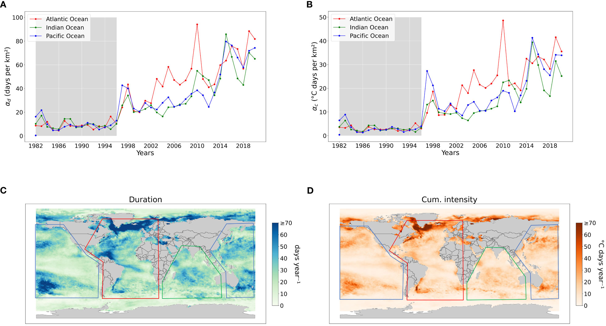
Figure 1 Properties of marine heat waves with fixed baseline (Dataset: NOAA OISST V2 (1982-2020), Threshold: 95^th percentile, Spatial resolution: 1°, Baseline: 1982-1996), (A) Regional average number of MHW days per km² (α_d), (B) Regional average cumulative intensity rel. threshold per km² (α_c), (C) Average number of MHW days per year (i.e., the sum of all MHW days divided by the total number of years), (D) Average cumulative intensity per year (i.e., the sum of cumulative intensity divided by the total number of years). The shaded region in A and B signify the climatological period used to calculate MHWs, which is also employed in (C, D).

Marine organisms can adapt to temperature changes, hence the detection and evaluation of MHWs impacts based on the absolute baseline described above may overestimate the impacts of temperature extremes on phytoplankton communities. Hence, we have used a shifting baseline considering an 8-year rolling period. Note that the rolling period is selected to have an identical split over the period of 39 years. These shifting baselines have been used to detect and classify different MHWs given their attributes (duration, maximum and cumulative intensity, rate of onset, and rate of decline). Specifically, using a 95th percentile threshold over the baselines for detection, the temporal range of 1982-1989 is used as a baseline to calculate MHWs for the years 1989-1996, while 1982-1996 for the years 1997-2005, 1982-2005 for 2006-2013, and finally 1982-2013 for 2014-2020. This provides more conservative assessments of extreme MHWs and biologically sound reference values accounting for the possible adaptation of marine communities to long-term temperature increases. Additionally, the 8-year shifting window enables us to account for the decadal changes of westerly winds, temperatures and ocean gyres circulations (Oviatt et al., 2015).

2.3 Classification of MHWs

To address the spatio-temporal complexities of MHWs, we tested a range of methodologies to identify the significant characteristics and assemble them into different groups. As a preliminary measure, we employed principal component analysis (PCA) as a feature extraction method to understand ocean dynamics based on MHWs. Additionally, we also implemented distance and density-based clustering methods such as KMeans (Zhang et al., 1996) and BIRCH (Syakur et al., 2018), owing to their capability to manage a large volume of samples. However, the KMeans clustering algorithm proved to be an effective approach for identifying the relevant features of MHWs and classifying them into separate groups based on feature similarities. This algorithm takes MHW features, namely duration, maximum intensity, rate onset and rate decline, as input vectors and applies clustering in the 4-dimensional feature space where each data point represents an MHW event. Please note that all the MHWs features are standardized because unequal variances can put more weight on variables with smaller variances. The clustering analysis uses a heuristic approach, the elbow method, to determine the optimal cluster count based on a distortion score (Zach, 2023). This score is calculated as an average of the square of distances from the cluster center to data points associated with each respective cluster. The algorithm is set to minimize variance in each cluster based on squared Euclidean distances where data are normalized (between 0 and 1) using min-max normalization. The optimal cluster count is the point after which decreasing trend in the distortion score becomes constant.

2.4 Parameter computation and statistical testing

Various parameters were employed to examine the spatio-temporal trends of MHWs across different figures. Regional yearly values (α) of duration and cumulative intensity are calculated considering the total area exposed to MHWs, thus:

$\begin{array}{ll}\alpha =\frac{{\sum }_i^R{X}_i^d·A_i}{A_R},& (2)\end{array}$

where R is the total number of grid cells in each region (i.e., Atlantic, Pacific, Indian Ocean), $A_i$ is the area ($k{m}^2$) of each cell, $A_R$ represents the area of the entire region ($k{m}^2$), and $X$ is the variable of interest calculated annually for each pixel which can either be duration ($days/k{m}^2$) or cumulative intensity (°C days/km²) of the MHWs. This makes the time series of the above-mentioned variables comparable across different regions. For spatial distributions, the average values for each grid cell are computed by dividing their total (across the period considered) by the total number of years, typically from 1982 to 2020 (see section 4.1). However, when using the 8-year rolling baseline, the considered periods differ and the total is divided by the specific number of years included in the summation (generally over the period 1989-2020). Additionally, the relative frequency ($\gamma$) of a variable for each grid cell is calculated by dividing the total within a specific time period by the total in the entire cluster over all time periods.

We employed two statistical tests—Welch’s test and the Mann-Whitney test to investigate whether detected MHWs’ impacts on phytoplankton are statistically significant. Welch’s test evaluates the means of two data groups to ascertain if a statistically significant distinction exists between them. This test presumes a normal data distribution while not assuming equal variances between the two groups. Conversely, the Mann-Whitney test assesses the medians of two data sets to identify if a statistically significant difference is present, without making assumptions about a specific data distribution or equal variances. Both tests yield p-values that are used to determine the statistical significance of the observed differences. In this research, we have used a predetermined significance level (i.e., p_value = 0.05) to reject or fail to reject the null hypothesis where the null hypothesis suggests that there is no significant difference between the two distributions. Additionally, to comprehend the changes in these distributions, we used the skewness index. The value of skewness indicates the extent to which the distribution is stretched or skewed in either direction; a positive value signifies a right-skewed distribution and vice versa.

3 Results

3.1 Marine heat waves frequency and distribution

On average, the duration of MHWs and MHW cumulative intensity have increased substantially on a global scale as well as in different regions (Figure 1). During the considered baseline period (1982-1996), the average duration and cumulative intensity of MHWs were consistently less than 20 days and 10°C days, respectively, with small yearly variations (Figures 1A, B). Note that, the calculation of MHWs during the baseline period provides a conservative estimate of MHW duration and intensity, as this period falls within the climatology period. After 1996, both duration and cumulative intensity have shown increasing trends across all regions. Using statistical tests (as in Section 2.4), we found that the duration and cumulative intensity are significantly different among all the regions (see Appendix 5, Table 3). The Pacific region witnessed two sudden increases in MHWs during 1997-1998 and 2014-2015 which can be associated to El Niño events. The Atlantic region has seen a constant increase in both duration and intensity having 2010 as the year with the highest number of MHW days and cumulative intensity on record. Lastly, the Indian Ocean has followed similar trends as the Pacific with similar duration but comparatively lower cumulative intensity values (Figures 1A, B).

Temperate and polar regions are characterized by up to more than 70 days per year of MHWs (Figure 1C) with relatively high intensity (Figure 1D). In the North and South Pacific, numerous areas experience more extended periods and greater intensity of marine heatwaves (MHWs) compared to other surrounding regions. In the Atlantic Ocean, the northern boundary of the North Atlantic sub-polar gyre and the Eastern Greenland shelf show MHW duration that is substantially longer than the average values for the entire Atlantic Ocean (Figure 1C), whereas high cumulative intensity MHWs are predominantly super-positioned with highly dynamic regions such as Gulf Stream, Labrador current, East-Greenland current, Brazilian current and Agulhas Retroflection region (Figure 1D). Furthermore, regions like the Caribbean sea and the north coast of South America seem to have longer but less intense MHWs, which might indicate different drivers occurring in those areas. Other regions like the Baltic sea, east-Mediterranean sea, east-Black sea, Caspian sea and Tasman sea also have relatively longer duration and high-intensity MHWs.

3.2 Classification of MHWs

Using the 8-year rolling window baseline, we have computed MHWs for each period (Figure 2A) and classified them based on their physical attributes. This classification involved testing different clustering methods and combinations of attributes (more details provided in the discussion in Section 4). The KMeans approach provided a clearer distinction between clusters, when duration, maximum intensity, rate of onset and rate of decline were considered (Figure 2B). Three emerging clusters could be associated with three types of MHWs which we have labelled as Moderate, Abrupt and intense, and Extreme MHWs, respectively (Table 1). Note that the labelling of these clusters was determined here only by the characteristics of the cluster’s features. Moderate MHWs are characterized by low range values for all features, while abrupt and intense MHWs exhibit high maximum intensity, high rate of onset, and high rate of decline. Extreme MHWs represent those with both extended durations and high intensities. While the clusters are not wholly isolated in terms of projected attributes, as there are some MHWs from each cluster located in the overlapping zone (Figure 2B), they are still clearly distinct based on all the considered attributes. Moderate MHWs predominantly exist in this zone followed by abrupt and intense MHWs. However, Extreme MHWs have the biggest range of duration and max intensity whereas moderate MHWs have the smallest range despite having the highest percentage of MHWs (Table 1).

TABLE 1

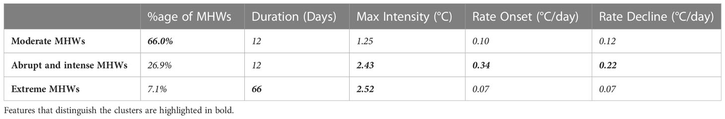
Table 1 Characterizations of the clusters identified by the KMeans and represented using centroid values.

FIGURE 2

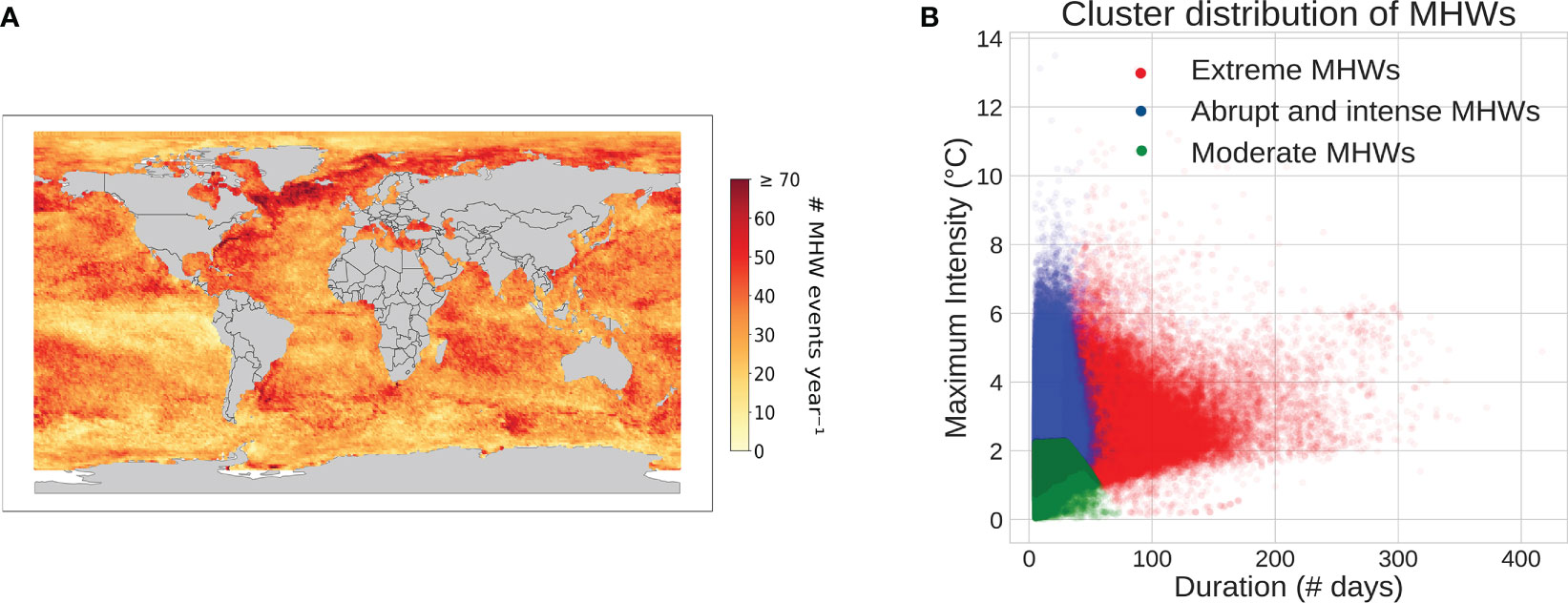
Figure 2 Spatial distribution of MHWs with an 8-year rolling baseline, (A) Total number of MHW events across the different periods averaged on the total number of years (1989-2020). Note that, the range 1982-1988 was only used as an initial baseline without calculating MHWs, (B) Cluster projection of MHWs’ duration and maximum intensity.

The moderate MHWs cluster accounts for 66% of all MHWs (Table 1) and has a relatively short duration and small cumulative intensities. This group of MHWs ranges between 5 to 60 days in total with the cluster’s centroid (median) placed at 12 days duration, whereas max intensity ranges from 0.02°C to 2.2°C (Figure 2B) above threshold with a median of 1.25°C. These MHWs undergo slow rates of increase and decline in intensities with values around 0.1°C/day (Table 1). Moderate MHWs typically can occur everywhere and cover most of the global ocean where regions like the East Greenland shelf and Norwegian sea, Caribbean sea, Philippine sea, etc., have a high frequency which accounts for more than 30 days per year (Figure 3A).

FIGURE 3

Figure 3 Spatial distribution of three MHW categories namely, (A) Moderate MHWs; (B) Abrupt and Intense MHWs; (C) Extreme MHWs, displaying the total number of MHW days normalized by the numberof years considered (i.e., 1989-2020). Note that, the total number of MHWs across the three categories isthe same of Figure 2A.

Abrupt and intense MHWs show up as 26.9% of all MHWs which have a distinct behavior of high increase and decline rates as well as relatively elevated maximum intensities with a median value of 2.43°C (Table 1). These MHWs are characterized by a similar range of duration as the moderate MHWs but with high variance in intensity levels which ranges between 0.5°C and 8°C (Figure 2B). These MHWs are most commonly found in the highly dynamic ocean regions, i.e., along western boundary currents including the gulf stream and neighbor areas, Kuroshio current, Agulhas Retroflection and Brazil-Malvinas confluence (Figure 3B). The abrupt and intense MHWs are also commonly present in the East Australian Current Extension and Leeuwin Current regions, which are affected by strong poleward advection and mesoscale dynamics (Sen Gupta et al., 2020).

Extreme MHWs are less frequent (7.1% of all MHWs) but persist for longer duration and high intensities with a median of 66 days and 2.52°C respectively (Table 1). In terms of duration and intensity, the most extreme MHWs are typically found to occur over a range of 40 to 200 days and exhibit temperatures between 1 °C and 7°C. These MHWs are characterized by slow rates of onset and decline with the values of 0.07° C/day. In general, temperate and polar regions seem to have more extreme MHWs than other regions. Especially the western and eastern Greenland show relatively high frequency for extreme MHWs, but the relatively high frequency is also shown in other areas of the Atlantic Ocean including the North Atlantic Subpolar Gyre (NASPG), the N-W Atlantic, as well as along the Brazilian current (Figure 3C). In the Pacific, the so-called Blob region shows ≥ 30 days per year of extreme MHWs and the Tasman sea and the western part of the South Pacific gyre have also witnessed these extremes, with most of the episodes occurring during the El Nino periods.

3.3 Temporal and spatial variations of extreme MHWs

The temporal and spatial dynamics of the extreme MHWs can be investigated by looking at the changes in their spatial distribution within the different periods included in the 8-year shifting baseline analysis (Figure 4). It can be inferred that these extreme MHWs are becoming more and more frequent over time (Figure 4). During 1989-1996 (the first period in the analysis), Extreme MHWs occur seldom and on the edges of the North Pacific and North Atlantic gyres and along Kuroshio and subarctic currents (Figure 4A). During 1997-2004, those events are still quite infrequent although eastern Greenland and Iceland show a substantial increase in these extreme events. It is worth noting that the strong El-Niño event (1997-1998) is also slightly visible in this period (Figure 3B). Between the years 2005 and 2012, there was a substantial increase in the occurrence of extreme MHWs worldwide, with a particularly sharp increase observed in the Atlantic Ocean. The relative frequency (γ) of these events ranged from 0.8 to 1 in both the northern and southern regions and across both coastal and open ocean areas (Figure 4C). The area of the Labrador sea shows as a largely affected area by extreme events with an average duration of around 70 days year-1 and maximum intensity of 3.5°C within this 8-year period (2005-2012). The 2013-2020 period has recorded the highest number of extreme MHWs when using a baseline calculated over the 1982-2012 period. Some of these events are well known like ‘The Blob (2014-2016)’ in the Pacific, the North-West Atlantic region warming and the intense Indian Ocean warming (Figure 4D). Relatively intense and frequent extremes can also be observed in the Mediterranean and the Tasman Sea.

FIGURE 4

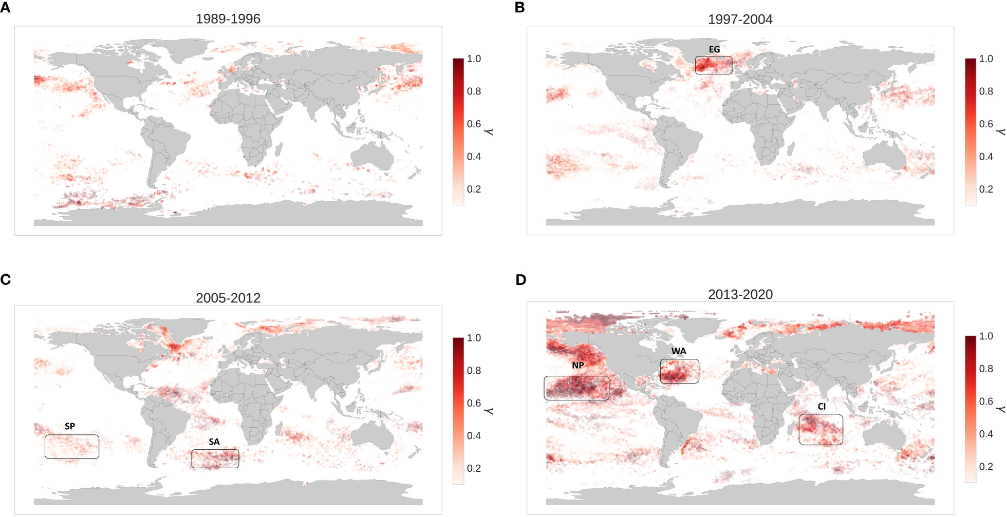
Figure 4 Distribution of Extreme MHWs across the different periods (A) 1989-1996, (B) 1997-2004, (C) 2005-2012, (D) 2013-2020. The color bar represents the relative frequency (γ) which is a ratio of extreme MHWs in a specific period and all extreme MHWs in the same cluster for all periods. Furthermore, regions with a less number of MHW events exhibit greater transparency than those with more MHW events. Areas of interest to assess the impacts on phytoplankton dynamics are indicated with the black boxes.

3.4 Impact of extreme MHWs on phytoplankton

To study the impact of extreme MHWs on marine plankton communities, we focused on regions emerging as frequently affected by those extreme events. Based on the results in Figure 4 we selected 6 regions namely, East Greenland(EG), West Atlantic(WA), South Atlantic(SA), Central Indian(CI), North Pacific(NP) and South Pacific(SP) which are analyzed in the Figure 5.

FIGURE 5

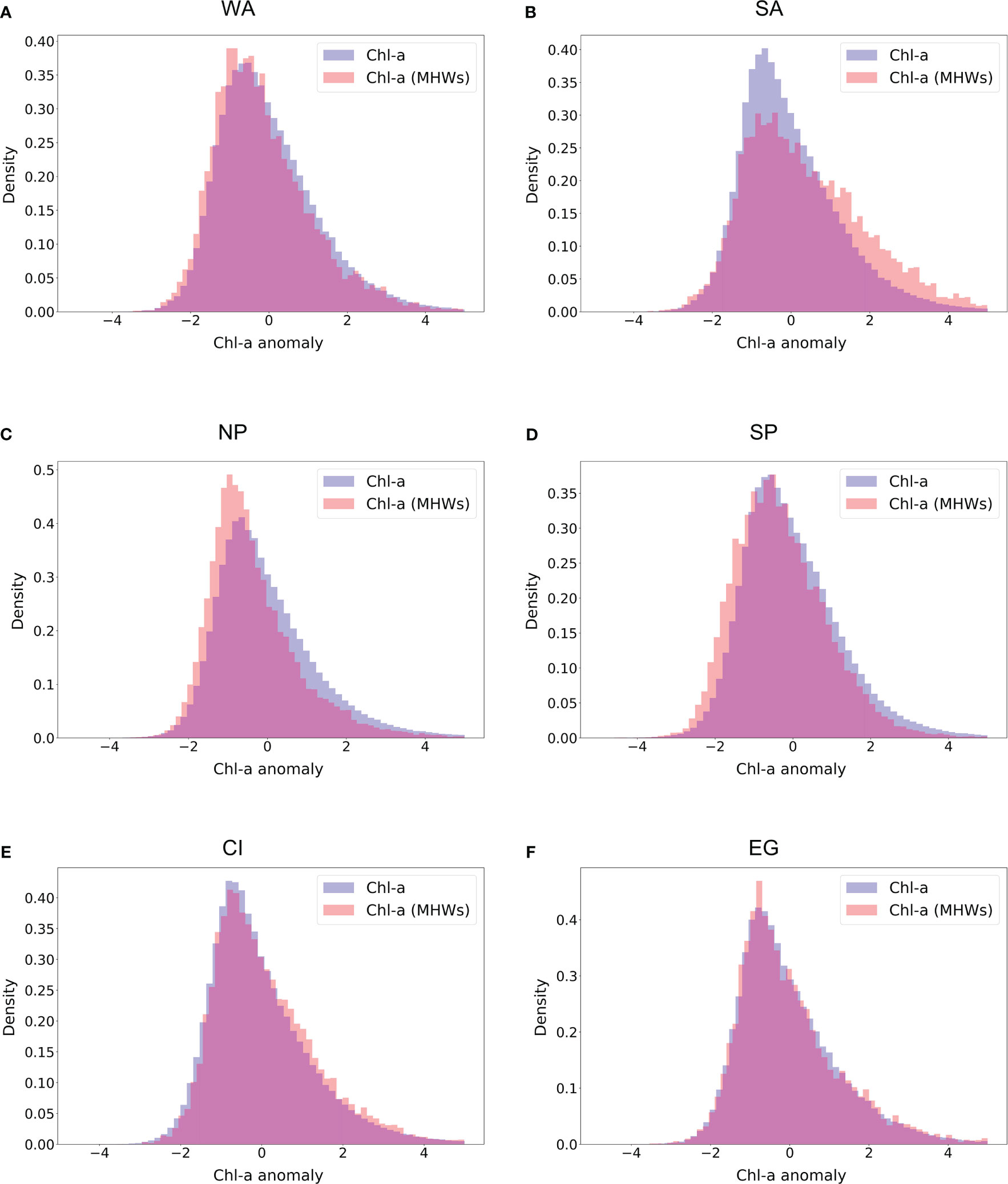
Figure 5 Density distribution of chl-a anomalies calculated using the method mentioned in 3.1. Blue color represents the total chl-a anomaly in the whole region; Orange color shows the chl-a anomaly in the presence of extreme MHWs; Purple color is the distribution overlap between total chl-a anomaly and the presence of extreme MHWs. Regions are identified as (A) West Atlantic(WA) Region, (B) South Atlantic(SA) Region, (C) North Pacific(NP) Region, where (D) South Pacific(SP) Region (E) Central Indian(CF) Region and (F) East Greenland (EG region). Note that, the chl-a anomaly distribution for each region represents the time period of 23 years (1998-2020).

The co-existence of extreme MHWs and chl-a anomalies is analyzed with respect to their general distribution in those specific regions. The anomalies are calculated based on the method presented in section 2.1. The distributions of chl-a in all the regions are slightly right-skewed (with a skewness index ranging from 0.5 to 1.5). This observation indicates the overall higher frequency of negative chl-a anomalies and is also the case when only anomalies within extreme MHW periods are considered (i.e., chl-a(MHW), Figure 5). The shift in frequency of chl-a anomalies in the presence of MHWs is relatively minor when extreme MHWs are present. The impact of those shifts can be considered marginal in terms of the effects on the ecology of plankton. Nevertheless, statistical tests (i.e., Welch’s test, and Mann-Whitney test) show that the shift is significant in most regions and yields remarkably low p-values. It is important to consider that the high number of samples in each region does cause the tests to be sensitive to differences between means, thus resulting in extremely low p-values. Further details on the statistical tests can be found in the Appendix (Appendix 5; Table 2).

Regions in Figures 5A, B lie in the North (WA) and South (SA) Atlantic Ocean respectively. In the WA region, the density distribution of the chl-a anomaly displays a slightly negative shift in the presence of extreme MHWs (Figure 4A) whereas the SA region shows a flatter curve with a small positive shift in the presence of extreme MHWs (Figure 5B). In the Pacific Ocean (NP and SP regions), chl-a anomaly distribution in both regions shows a clear negative shift in the presence of extreme MHWs (Figures 5C, D) indicating a comparatively strong correlation between extreme MHWs and phytoplankton productivity. On the other hand, other regions like CI (in the Indian Ocean close to the equator) and EG (a polar region in the north Atlantic ocean) do not show any significant shift in chl-a anomalies distribution with MHWs presence (Figures 5E, F). Furthermore, the details of the spatio-temporal variability of chl-a anomaly and extreme MHWs can largely vary across regions (Appendix 1-3).

4 Discussion and conclusion

Several studies have raised the issue of the effects of frequent occurrences and severity of global MHWs over the last few decades. However, results show high regional variability, with some areas being more prone to extreme warming than others, and different effects of extreme events across different ocean regions (Holbrook et al., 2019; Spillman et al., 2021). Therefore, we analyzed the temporal trends of extreme events across the global ocean. Based on the Extended Reconstructed Sea Surface Temperature (ERSST) dataset, Huang et al. (2018) observed relatively stable SST from mid-20th century until 1980, followed by a linear rise in and after the 1980s. However, the last 3 decades have seen some severe transitions in ocean warming, resulting in years 2014 to 2020 being the hottest years globally across the oceans (Figure 1). Besides these years, several other prominent shifts occurred where MHWs days and intensity shifts have been recorded in the years 1997-1998, 2010-2011 and 2014-2015 (Figures 1A, B) across different ocean regions (i.e., Pacific, Atlantic, Indian). These events are typically driven by some large-scale and regional climatic modes like El Nino, regional processes like shallow mixed layers in summers, anomalous high-pressure systems, suppressed wind speeds and vertical mixing, and subsurface processes like heat advection (Sen Gupta et al., 2020).

Events detected in our analyses have been reported in the past (Pearce and Feng, 2013; Chen et al., 2014; Bond et al., 2015; Di Lorenzo and Mantua, 2016; Oliver et al., 2017; Benthuysen et al., 2018) and are considered to be linked to various drivers in different regions (Holbrook et al., 2019; Sen Gupta et al., 2020). Some of the drivers suggested are the evolution of sub-polar gyres, heat content anomalies and negative North Atlantic oscillations (NAO) which have significantly affected the Atlantic Ocean (Robson et al., 2012). Besides that, El Nino also played a significant role as an MHW driver in 1997-1998. During these years, as well as the period from 2014-2015, the Pacific Ocean experienced extended periods of intense warming, leading to major shifts in Sea Surface Temperature (SST). In the Indian Ocean, warming is typically linked with a negative North Atlantic Oscillation (NAO) and a positive Indian Ocean Dipole (IOD) in the western and central regions. Moreover, post-El Nino periods also had significant effects on the south- east Indian Ocean (Saranya et al., 2022). Other studies (Marin et al., 2022) have suggested that the onset and decay of MHWs in tropical regions are mainly governed by air-sea heat fluxes (ASHF), whereas the heat advection plays a significant role as MHW driving force in sub-tropical regions. As per the temperate zones, where seasonal variability is much higher compared to the tropics, interactions between multiple drivers become more complex and challenging. Some authors (Sparnocchia et al., 2006; Olita et al., 2007; Chen et al., 2014; Holbrook et al., 2019) have analyzed various drivers like mesoscale-eddy activities, ocean gyre circulations, ASHF, reduction in wind speed, Ekman pumping, atmospheric circulation and pressure anomalies etc. which supported some of the most detrimental MHWs like Mediterranean MHW 2003, North-West Atlantic MHW 2012 and North-East Pacific MHW 2013-2016 with El-Nino.

To categorize marine heatwaves (MHWs) into distinct groups, we evaluated various classification techniques, including PCA, BIRCH, and KMeans. PCA was able to account for approximately 90% of the variance using three principal components (PCs) but only succeeded in identifying regions with high PC scores that could be linked to upwelling and highly dynamic regions (refer to Figure 9 in Appendix 4). To efficiently apply the BIRCH algorithm, we adjusted the threshold parameter using k-fold validation based on silhouette scores. Nevertheless, even with the optimal threshold selected, the algorithm was unable to effectively classify MHWs (see Figure 10 in Appendix 4). On the other hand, KMeans demonstrated its effectiveness in recognizing relevant MHW features and classifying them into distinct categories. Notably, this method was able to group MHWs into three different classifications (labelled moderate, abrupt and intense, and extreme MHWs), which aligns with the traditional means of distinguishing biological extremes. The most extreme MHWs were found to be clustered in areas where past significant heat events have occurred, further corroborating the validity of this approach.

Results from Marin et al. (2022); Hayashida et al. (2020) show that Moderate MHWs are likely driven by the mixed contributions of local (advection, eddy heat flux, air-sea exchanges, etc.) and large-scale (ocean gyre oscillations, oceans dipoles, ENSO Etc.) climate modes which control heat variations over small and different spatio-temporal scales. This indicates very high complexity and the interactions between these different drivers can potentially be addressed using deep neural networks in the future. Extreme MHWs have typically been associated with regions where these events can be explained by the contribution of ASHF, ocean heat advection and other local processes like turbulent mixing, and thermocline deepening, as well as likely driven by temporary shifts in permanent ocean currents bringing warmer waters into higher latitude colder regions (Holbrook et al., 2019; Sen Gupta et al., 2020; Marin et al., 2022).

The increasing frequency of MHWs is believed to have an important role in influencing the marine ecosystem over time. These MHWs are disrupting the ecosystem balance by a redistribution of marine biogeography and changing the habitat ranges of certain species. Recent analyses (Arteaga and Rousseaux, 2023) suggested that the extremely warm conditions during the 2016 El Nino event led to a significant reduction of approximately 40% in surface chlorophyll concentrations in the Pacific Ocean as well as major changes in phytoplankton community structure. Considering the adaptive nature of marine organisms, we assumed that extreme MHWs calculated using a shifting baseline could have a tangible impact on phytoplankton distribution. Since these extreme MHWs are increasing over time (Figure 4) and across the globe, it can alter population growth and community structure in phytoplankton (Gao et al., 2021; Harvey et al., 2022; Arteaga and Rousseaux, 2023; Doni et al., 2023). Moreover, the use of a shifting baseline, instead of a fixed reference, could enhance the analysis of phytoplankton adaptation to ocean warming, such as an increase in their maximum critical thermal limit (Jin and Agustí, 2018). Indeed, expanding the baseline for MHWs closer to the period analyzed for impacts provided a more conservative estimate of the effects of warming. On the other hand, phytoplankton anomalies have been calculated using a fixed reference frame as no clear seasonal trend was observed within the considered regions. Therefore, we considered a single baseline for phytoplankton including the entire period of 23 years (monthly values for the range 1998-2020) and deviations from this long-term climatology are used as chl-a anomalies. The results presented in Figure 5 are nonetheless robust to changes in baselines for chl-a anomalies.

To understand the impact of Extremes MHWs on phytoplankton, we have analyzed six regions located in the Atlantic, Pacific and Indian Oceans, and calculated the changes in chl-a anomalies over time in the presence of extreme MHWs. The selection of regions was driven by the relatively high frequency of Extreme MHWs in those areas (Figure 4). Although the selection process was subjective, it effectively incorporated regions with a significant occurrence of extreme MHWs to assess their impacts. It should be noted that expanding the size of the regions (thus including more non-impacted areas) would not significantly change the frequency distributions of chl-a anomalies. Additionally, keeping those regions small is important to avoid the confounding effects of multiple drivers. Results from Figure 5 showed that regions in the Pacific Ocean have a stronger negative correlation between chl-a anomalies and extreme MHWs. However, temperate regions in the Atlantic Ocean show contrasting results where chl-a anomalies in WA and SA regions have negative and positive shifts respectively, in the presence of extreme MHWs. Furthermore, two other regions (CI and EG) do not give any clear results on the interactions between chl-a anomalies and MHWs.

Our results from specific regions such as WA, NP and SP are consistent with other findings (e.g., Ajani et al. (2020) and Doney (2007)). The SA region is situated at the intersection between the South Atlantic Gyre’s boundary current and the Antarctic Circumpolar Current and changes in this front can significantly impact the distribution of temperature, nutrients, and consequently phytoplankton productivity. It has been shown that MHWs are closely associated with changes in the global currents (Todd et al., 2019). Concurrently, these currents can induce upwelling, transporting nutrient-rich waters to the surface and supplying vital nutrients that promote phytoplankton growth (McClain et al., 2004). The CI region lies close to the equator hence in a region that is strongly stratified throughout the year, hence surface phytoplankton concentration as detected by remote sensing may not accurately represent the total concentration within the water column. Consequently, our detection of the impacts of MHWs in this region using satellite data could potentially introduce biases in the analyses as previously suggested (McClain et al., 2002). The polar region, such as the EG we have chosen for our study, generally has very complex dynamics driven by various atmospheric, ocean and ice processes which may have significant impacts on ocean stratification (Nummelin et al., 2016; von Appen et al., 2021). Besides, the EG region also includes part of the North Atlantic subpolar gyre which influences a range of processes, such as shallow mixing and front dynamics. The interlink between these processes plays a dominant role in defining MHWs and phytoplankton productivity making it difficult to disentangle the interactions (Richardson and Schoeman, 2004).

MHWs can be triggered by various physical factors, including moving fronts, shallower mixed layers, increased stratification, and persistent eddy structures (Sen Gupta et al., 2020). These factors can also directly influence the local food web, leading to alterations in phytoplankton and chlorophyll anomalies. Our findings suggest that MHWs can serve as both a driver and an indicator of changes in phytoplankton dynamics, alongside other drivers that can generate similar anomalies. Nonetheless, it could be speculated that as the frequency and intensity of MHWs continue to rise, they may become a dominant factor driving thermal regimes outside the adaptive capability of different phytoplankton groups, thus significantly affecting phytoplankton dynamics and community structure. This could lead to cascading effects in marine food webs including changes in the availability and quality of food resources as well as the transfer to higher trophic levels, such as zooplankton, fish, and marine mammals. Therefore, further understanding of the direct effects of MHWs on marine ecosystems is crucial for predicting and mitigating their potential impacts.

Data availability statement

Sea surface temperature (SST) and phytoplankton concentration (chl-a) data used in this research are publicly available from NOAA and marine copernicus respectively. SST: https://psl.noaa.gov/data/gridded/data.noaa.oisst.v2.highres.html Chl-a: https://data.marine.copernicus.eu/products SST: https://psl.noaa.gov/data/gridded/data.noaa.oisst.v2.highres.html Chl-a: https://data.marine.copernicus.eu/products.

Author contributions

All the authors contributed to the conceptualization and methodology of the process involved in this paper which led to our findings. AnC is responsible for the data curation and application of statistical and computational techniques which are used for analysis. Furthermore, He is also responsible for the implementation of supporting algorithms, data visualization and writing the original draft. PM acted as the main supervisor and was actively involved in project administration. PM, FR, and AsC contributed by providing study materials and data resources, validation and verification of results whereas PS actively contributed to providing ideas during the implementation process. MS was one of the main contributors to the ideation of the project. All authors contributed to the article and approved the submitted version.

Funding

This article is delivered under the MISSION ATLANTIC project funded by the European Union’s Horizon 2020 Research and Innovation Program under grant agreement No. 639 862428.

Conflict of interest

The authors declare that the research was conducted in the absence of any commercial or financial relationships that could be construed as a potential conflict of interest.

Publisher’s note

All claims expressed in this article are solely those of the authors and do not necessarily represent those of their affiliated organizations, or those of the publisher, the editors and the reviewers. Any product that may be evaluated in this article, or claim that may be made by its manufacturer, is not guaranteed or endorsed by the publisher.

Supplementary material

The Supplementary Material for this article can be found online at: https://www.frontiersin.org/articles/10.3389/fmars.2023.1177571/full#supplementary-material

References

Ajani P. A., Davies C. H., Eriksen R. S., Richardson A. J. (2020). Global warming impacts micro-phytoplankton at a long-term pacific ocean coastal station. Front. Mar. Sci. 7. doi: 10.3389/fmars.2020.576011

CrossRef Full Text | Google Scholar

Arteaga L. A., Rousseaux C. S. (2023). Impact of pacific ocean heatwaves on phytoplankton community composition. Commun. Biol. 6, 263. doi: 10.1038/s42003-023-04645-0

PubMed Abstract | CrossRef Full Text | Google Scholar

Benthuysen J. A., Oliver E. C. J., Chen K., Wernberg T. (2020). Editorial: advances in understanding marine heatwaves and their impacts. Front. Mar. Sci. 7. doi: 10.3389/fmars.2020.00147

CrossRef Full Text | Google Scholar

Benthuysen J. A., Oliver E. C. J., Feng M., Marshall A. G. (2018). Extreme marine warming across tropical australia during austral summer 2015–2016. J. Geophys. Res.: Oceans. 123, 1301–1326. doi: 10.1002/2017JC013326

CrossRef Full Text | Google Scholar

Bond N. A., Cronin M. F., Freeland H., Mantua N. (2015). Causes and impacts of the 2014 warm anomaly in the ne pacific. Geophys. Res. Lett. 42, 3414–3420. doi: 10.1002/2015GL063306

CrossRef Full Text | Google Scholar

Brodeur R. D., Auth T. D., Phillips A. J. (2019). Major shifts in pelagic micronekton and macrozooplankton community structure in an upwelling ecosystem related to an unprecedented marine heatwave. Front. Mar. Sci. 6. doi: 10.3389/fmars.2019.00212

CrossRef Full Text | Google Scholar

Cavole L. M., Demko A. M., Diner R. E., Giddings A., Koester I., Pagniello C. M. L. S., et al. (2016). Biological impacts of the 2013–2015 warm-water anomaly in the northeast pacific: winners, losers, and the future. Oceanography 29, 273–285. doi: 10.5670/oceanog.2016.32

CrossRef Full Text | Google Scholar

Chen K., Gawarkiewicz G. G., Lentz S. J., Bane J. M. (2014). Diagnosing the warming of the northeastern u.s. coastal ocean in 2012: a linkage between the atmospheric jet stream variability and ocean response. J. Geophys. Res.: Oceans. 119, 218–227. doi: 10.1002/2013JC009393

CrossRef Full Text | Google Scholar

Cheung W. W. L., Frölicher T. L., Lam V. W. Y., Oyinlola M. A., Reygondeau G., Sumaila U. R., et al. (2021). Marine high temperature extremes amplify the impacts of climate change on fish and fisheries. Sci. Adv. 7, eabh0895. doi: 10.1126/sciadv.abh0895

PubMed Abstract | CrossRef Full Text | Google Scholar

Collins M., Sutherland M., Bouwer L., Cheong S.-M., Froülicher T., DesCombes H. J., et al. (2019). Extremes, abrupt changes and managing risk. IPCC Special Report on the Ocean and Cryosphere in a Changing Climate, 589–655. doi: 10.1017/9781009157964.008

Google Scholar

Deguette A., Barrote I., Silva J. (2022). Physiological and morphological effects of a marine heatwave on the seagrass cymodocea nodosa. Sci. Rep. 12.

PubMed Abstract | Google Scholar

Di Lorenzo E., Mantua N. (2016). Multi-year persistence of the 2014/15 north pacific marine heatwave. Nat. Climate Change 6, 1042–1047. doi: 10.1038/nclimate3082

CrossRef Full Text | Google Scholar

Doney S. (2007). Oceanography - plankton in a warmer world. Nature 444, 695–696. doi: 10.1038/444695a

CrossRef Full Text | Google Scholar

Doni L., Oliveri C., Lasa A., Di Cesare A., Petrin S., Martinez-Urtaza J., et al. (2023). Large-Scale impact of the 2016 marine heatwave on the plankton-associated microbial communities of the great barrier reef (australia). Mar. Pollut. Bull. 188, 114685. doi: 10.1016/j.marpolbul.2023.114685

PubMed Abstract | CrossRef Full Text | Google Scholar

Elise Beaudin A. B. (2022). How marine heatwaves impact life in the ocean. Front. Young. Minds.

Google Scholar

Frölicher T. L., Fischer E. M., Gruber N. (2018). Marine heatwaves under global warming. Nature 560, 360–364. doi: 10.1038/s41586-018-0383-9

PubMed Abstract | CrossRef Full Text | Google Scholar

Gao G., Zhao X., Jiang M., Gao L. (2021). Impacts of marine heatwaves on algal structure and carbon sequestration in conjunction with ocean warming and acidification. Front. Mar. Sci. 8, 758651. doi: 10.3389/fmars.2021.758651

CrossRef Full Text | Google Scholar

Garrabou J., Gómez-Gras D., Ledoux J., Linares C., Bensoussan N., López-Sendino P., et al. (2019). Collaborative database to track mass mortality events in the mediterranean sea. Front. Mar. Sci. 6. doi: 10.3389/fmars.2019.00707

CrossRef Full Text | Google Scholar

Garrabou J., Gómez-Gras D., Medrano A., Cerrano C., Ponti M., Schlegel R., et al. (2022). Marine heatwaves drive recurrent mass mortalities in the mediterranean sea. Global Change Biol. doi: 10.1111/gcb.16301

CrossRef Full Text | Google Scholar

Gruber N., Boyd P. W., Frölicher T. L., Vogt M. (2021). Biogeochemical extremes and compound events in the ocean. Nature 600, 395–407. doi: 10.1038/s41586-021-03981-7

PubMed Abstract | CrossRef Full Text | Google Scholar

Harvey B. P., Marshall K. E., Harley C. D., Russell B. D. (2022). Predicting responses to marine heatwaves using functional traits. Trends Ecol. Evol. 37, 20–29. doi: 10.1016/j.tree.2021.09.003

PubMed Abstract | CrossRef Full Text | Google Scholar

Hayashida H., Matear R. J., Strutton P. G., Zhang X. (2020). Insights into projected changes in marine heatwaves from a high-resolution ocean circulation model. Nat. Commun. 11. doi: 10.1038/s41467-020-18241-x

PubMed Abstract | CrossRef Full Text | Google Scholar

Hobday A. J., Alexander L. V., Perkins S. E., Smale D. A., Straub S. C., Oliver E. C. J., et al. (2016). A hierarchical approach to defining marine heatwaves. Prog. Oceanogr. 141, 227–238. doi: 10.1016/j.pocean.2015.12.014

CrossRef Full Text | Google Scholar

Holbrook N. J., Scannell H. A., Sen Gupta A., Benthuysen J. A., Feng M., Oliver E. C. J., et al. (2019). A global assessment of marine heatwaves and their drivers. Nat. Commun. 10. doi: 10.1038/s41467-019-10206-z

CrossRef Full Text | Google Scholar

Huang B., Angel W., Boyer T., Cheng L., Chepurin G., Freeman J., et al. (2018). Evaluating sst analyses with independent ocean profile observations. J. Climate 31. doi: 10.1175/JCLI-D-17-0824.1

CrossRef Full Text | Google Scholar

Huang B., Liu C., Banzon V., Freeman E., Graham G., Hankins B., et al. (2021). Improvements of the daily optimum interpolation sea surface temperature (doisst) version 2.1. J. Climate 34, 2923–2939. doi: 10.1175/JCLI-D-20-0166.1

CrossRef Full Text | Google Scholar

Hughes T. P., Kerry J. T., Álvarez Noriega M., Álvarez Romero J. G., Anderson K. D., Baird A. H., et al. (2017). Global warming and recurrent mass bleaching of corals. Nature 543, 373–377. doi: 10.1038/nature21707

PubMed Abstract | CrossRef Full Text | Google Scholar

Jin P., Agustí S. (2018). Fast adaptation of tropical diatoms to increased warming with trade-offs. Sci. Rep. 8.

Google Scholar

Marin M., Feng M., Bindoff N. L., Phillips H. E. (2022). Local drivers of extreme upper ocean marine heatwaves assessed using a global ocean circulation model. Front. Climate 4. doi: 10.3389/fclim.2022.788390

CrossRef Full Text | Google Scholar

Marín-Guirao L., Entrambasaguas L., Ruiz J. M., Procaccini G. (2019). Heat-stress induced flowering can be a potential adaptive response to ocean warming for the iconic seagrass posidonia oceanica. Mol. Ecol. 28, 2486–2501. doi: 10.1111/mec.15089

PubMed Abstract | CrossRef Full Text | Google Scholar

McClain C. R., Christian J. R., Signorini S. R., Lewis M. R., Asanuma I., Turk D., et al. (2002). Satellite ocean-color observations of the tropical pacific ocean. Deep. Sea. Res. Part II.: Topical. Stud. Oceanogr. 49, 2533–2560. doi: 10.1016/S0967-0645(02)00047-4

CrossRef Full Text | Google Scholar

McClain C. R., Signorini S. R., Christian J. R. (2004). Subtropical gyre variability observed by ocean-color satellites. Deep. Sea. Res. Part II.: Topical. Stud. Oceanogr. 51, 281–301. doi: 10.1016/j.dsr2.2003.08.002

CrossRef Full Text | Google Scholar

Moore C., Mills M., Arrigo K., Berman-Frank I., Bopp L., Boyd P., et al. (2013). Processes and patterns of oceanic nutrient limitation. Nat. Geosci. 6, 701–710. doi: 10.1038/ngeo1765

CrossRef Full Text | Google Scholar

Nummelin A., Ilicak M., Li C., Smedsrud L. H. (2016). Consequences of future increased arctic runoff on arctic ocean stratification, circulation, and sea ice cover. J. Geophys. Res.: Oceans. 121, 617–637. doi: 10.1002/2015JC011156

CrossRef Full Text | Google Scholar

Olita A., Sorgente R., Natale S., Gaberšek S., Ribotti A., Bonanno A., et al. (2007). Effects of the 2003 european heatwave on the central mediterranean sea: surface fluxes and the dynamical response. Ocean. Sci. 3, 273–289. doi: 10.5194/os-3-273-2007

CrossRef Full Text | Google Scholar

Oliver E. C. J., Benthuysen J. A., Bindoff N. L., Hobday A. J., Holbrook N. J., Mundy C. N., et al. (2017). The unprecedented 2015/16 tasman sea marine heatwave. Nat. Commun. 8. doi: 10.1038/ncomms16101

CrossRef Full Text | Google Scholar

Oviatt C., Smith L., McManus M. C., Hyde K. (2015). Decadal patterns of westerly winds, temperatures, ocean gyre circulations and fish abundance: a review. Climate 3, 833–857. doi: 10.3390/cli3040833

CrossRef Full Text | Google Scholar

Pearce A. F., Feng M. (2013). The rise and fall of the “marine heat wave” off western australia during the summer of 2010/2011. J. Mar. Syst. 111-112, 139–156. doi: 10.1016/j.jmarsys.2012.10.009

CrossRef Full Text | Google Scholar

Piatt J. F., Parrish J. K., Renner H. M., Schoen S. K., Jones T. T., Arimitsu M. L., et al. (2020). Extreme mortality and reproductive failure of common murres resulting from the northeast pacific marine heatwave of 2014-2016. PloS One 15. doi: 10.1371/journal.pone.0226087

CrossRef Full Text | Google Scholar

Richardson A. J., Schoeman D. S. (2004). Climate impact on plankton ecosystems in the northeast atlantic. Science 305, 1609–1612. doi: 10.1126/science.1100958

PubMed Abstract | CrossRef Full Text | Google Scholar

Robson J., Sutton R., Lohmann K., Smith D., Palmer M. D. (2012). Causes of the rapid warming of the north atlantic ocean in the mid-1990s. J. Climate 25, 4116–4134. doi: 10.1175/JCLI-D-11-00443.1

CrossRef Full Text | Google Scholar

Rost B., Riebesell U., Burkhardt S., Sültemeyer D. (2003). Carbon acquisition of bloom-forming marine phytoplankton. Limnol. Oceanogr. 48, 55–67. doi: 10.4319/lo.2003.48.1.0055

CrossRef Full Text | Google Scholar

Ruiz J., Marín-Guirao L., García-Muñoz R., Ramos-Segura A., Bernardeau-Esteller J., Pérez M., et al. (2018). Experimental evidence of warming-induced flowering in the mediterranean seagrass posidonia oceanica. Mar. Pollut. Bull. 134, 49–54. doi: 10.1016/j.marpolbul.2017.10.037

PubMed Abstract | CrossRef Full Text | Google Scholar

Samuels T., Rynearson T. A., Collins S. (2021). Surviving heatwaves: thermal experience predicts life and death in a southern ocean diatom. Front. Mar. Sci. 8. doi: 10.3389/fmars.2021.600343

CrossRef Full Text | Google Scholar

Santoleri R. (2023). Detection, characterization and trends of marine heat waves in the global worming scenario: the careheat project. doi: 10.5194/egusphere-egu23-8961

CrossRef Full Text | Google Scholar

Santora J. A., Mantua N. J., Schroeder I. D., Field J. C., Hazen E. L., Bograd S. J., et al. (2020). Habitat compression and ecosystem shifts as potential links between marine heatwave and record whale entanglements. Nat. Commun. 11. doi: 10.1038/s41467-019-14215-w

CrossRef Full Text | Google Scholar

Saranya J. S., Roxy M. K., Dasgupta P., Anand A. (2022). Genesis and trends in marine heatwaves over the tropical indian ocean and their interaction with the indian summer monsoon. J. Geophys. Res.: Oceans. 127.

Google Scholar

Schlegel R. W., Darmaraki S., Benthuysen J. A., Filbee-Dexter K., Oliver E. C. (2021). Marine cold-spells. Prog. Oceanogr. 198, 102684. doi: 10.1016/j.pocean.2021.102684

CrossRef Full Text | Google Scholar

Seager R., Hoerling M., Schubert S., Wang H., Lyon B., Kumar A., et al. (2015). Causes of the 2011-14 california drought. J. Climate 28, 6997–7024. doi: 10.1175/JCLI-D-14-00860.1

CrossRef Full Text | Google Scholar

Sen Gupta A., Thomsen M., Benthuysen J. A., Hobday A. J., Oliver E., Alexander L. V., et al. (2020). Drivers and impacts of the most extreme marine heatwaves events. Sci. Rep. 10.

Google Scholar

Smale D., Wernberg T., Oliver E., Thomsen M., Harvey B., Straub S., et al. (2019). Marine heatwaves threaten global biodiversity and the provision of ecosystem services. Nat. Climate Change 9. doi: 10.1038/s41558-019-0412-1

CrossRef Full Text | Google Scholar

Somero G. N. (2020). The cellular stress response and temperature: function, regulation, and evolution. J. Exp. Zool. Part A.: Ecol. Integr. Physiol. 333, 379–397.

Google Scholar

Sparnocchia S., Schiano M. E., Picco P., Bozzano R., Cappelletti A. (2006). The anomalous warming of summer 2003 in the surface layer of the central ligurian sea (western mediterranean). Annales. Geophys. 24, 443–452. doi: 10.5194/angeo-24-443-2006

CrossRef Full Text | Google Scholar

Spillman C. M., Smith G. A., Hobday A. J., Hartog J. R. (2021). Onset and decline rates of marine heatwaves: global trends, seasonal forecasts and marine management. Front. Climate 3. doi: 10.3389/fclim.2021.801217

CrossRef Full Text | Google Scholar

Stipcich P., Marín-Guirao L., Pansini A., Pinna F., Procaccini G., Pusceddu A., et al. (2022). Effects of current and future summer marine heat waves on posidonia oceanica: plant origin matters? Front. Climate 4. doi: 10.3389/fclim.2022.844831

CrossRef Full Text | Google Scholar

Syakur M., Khotimah B., Rochman E., Satoto B. D. (2018). “Integration k-means clustering method and elbow method for identification of the best customer profile cluster,” in IOP conference series: materials science and engineering, vol. 336. (IOP Publishing), 012017.

Google Scholar

Todd R. E., Chavez F. P., Clayton (2019). Global perspectives on observing ocean boundary current systems. Front. Mar. Sci. 6. doi: 10.3389/fmars.2019.00423

CrossRef Full Text | Google Scholar

Vajedsamiei J., Wahl M., Schmidt A. L., Yazdanpanahan M., Pansch C. (2021). The higher the needs, the lower the tolerance: extreme events may select ectotherm recruits with lower metabolic demand and heat sensitivity. Front. Mar. Sci. 8. doi: 10.3389/fmars.2021.660427

CrossRef Full Text | Google Scholar

von Appen W., Waite A. M., Bergmann M., Bienhold C., Boebel O., Bracher A., et al. (2021). Sea-Ice derived meltwater stratification slows the biological carbon pump: results from continuous observations. Nat. Commun. 12. doi: 10.1038/s41467-021-26943-z

CrossRef Full Text | Google Scholar

Wernberg T., Bennett S., Babcock R. C., De Bettignies T., Cure K., Depczynski M., et al. (2016). Climate-driven regime shift of a temperate marine ecosystem. Science 353, 169–172. doi: 10.1126/science.aad8745

PubMed Abstract | CrossRef Full Text | Google Scholar

Zach (2023) Elbow method. Available at: https://www.statology.org/elbow-method-in-python/.

Google Scholar

Zhang T., Ramakrishnan R., Livny M. (1996). Birch: an efficient data clustering method for very large databases. ACM Sigmod. Rec. 25, 103–114. doi: 10.1145/235968.233324

CrossRef Full Text | Google Scholar

1 APPENDIX: WEST AND SOUTH ATLANTIC REGION

FIGURE 6

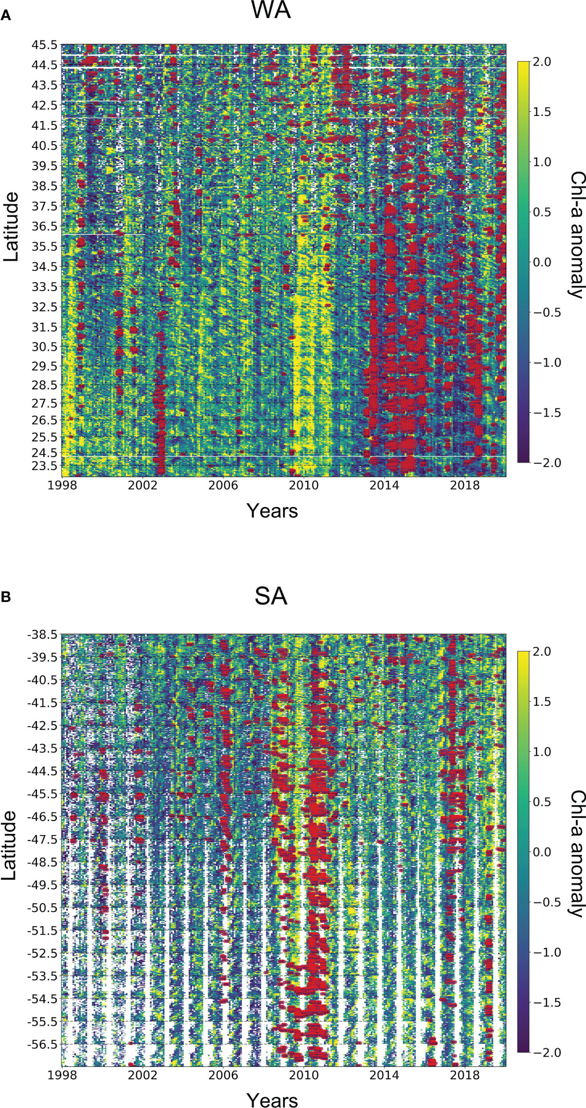
Figure 6 Spatio-temporal analysis of MHWs and Chl-a anomaly. Regions are flattened over the y-axis showing boundaries of latitudes, with each coordinate having time series on the x-axis. Furthermore, the chl-a anomaly is also super-positioned with extreme MHWs (red-coloured points). Note that, the empty spaces in A and B show the data gaps in chl-a anomaly.

2 APPENDIX: NORTH AND SOUTH PACIFIC REGION

FIGURE 7

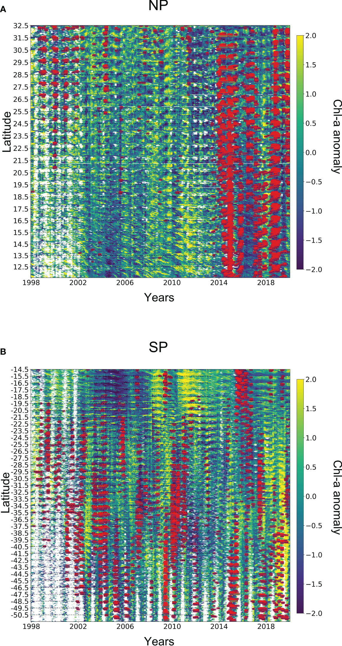
Figure 7 Spatio-temporal analysis of MHWs and Chl-a anomaly. Regions are flattened over the y-axis showing boundaries of latitudes, with each coordinate having time series on the x-axis. Furthermore, the chl-a anomaly is also super-positioned with extreme MHWs (red-coloured points). Note that, the empty spaces in A and B show the data gaps in chl-a anomaly.

3 APPENDIX: CENTRAL INDIAN AND EAST GREENLAND REGION

FIGURE 8

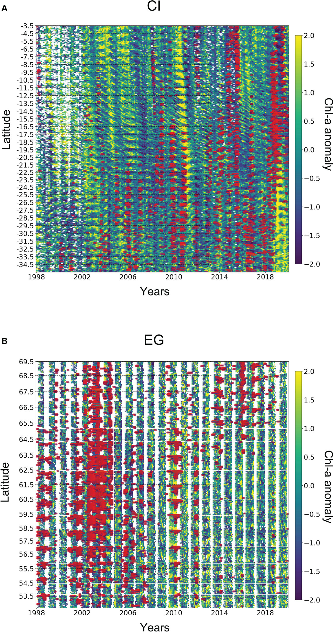
Figure 8 Spatio-temporal analysis of MHWs and Chl-a anomaly. Regions are flattened over the y-axis showing boundaries of latitudes, with each coordinate having time series on the x-axis. Furthermore, the chl-a anomaly is also super-positioned with extreme MHWs (red-coloured points). Note that, the empty spaces in A and B show the data gaps in chl-a anomaly.

4 APPENDIX: CLUSTERING ALGORITHMS

FIGURE 9

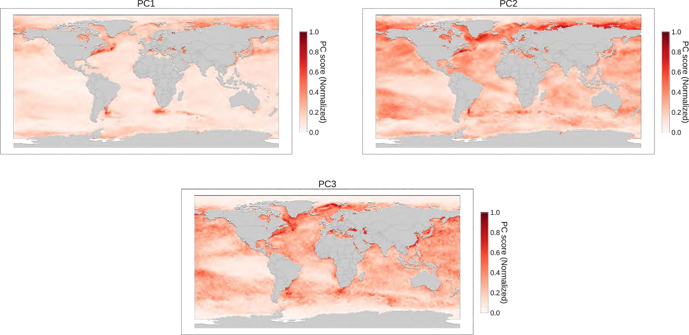
Figure 9 PCA clustering of MHWs

FIGURE 10

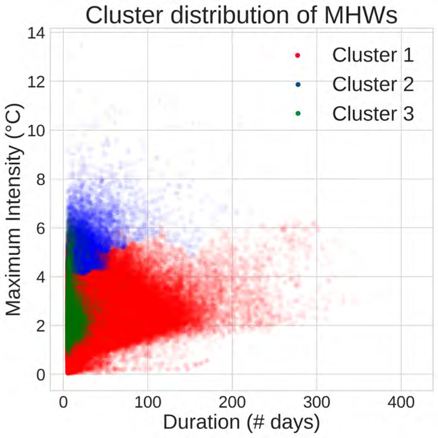
Figure 10 BIRCH clustering of MHWs

5 APPENDIX: STATISTICAL TESTS

Table 2. Statistical tests (p-values) distinguishing between total chlorophyll-a anomalies and chlorophyll-a anomalies observed during extreme MHWs.

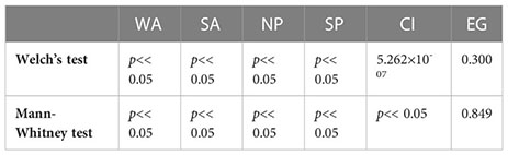
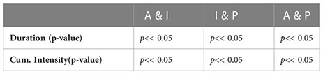
Table 3. Mann-Whitney test for analyzing the significant difference in duration and cumulative intensity across different regions, A, I and P represents Atlantic, Indian and Pacific Ocean respectively.