The large-scale impact of anthropogenic mixing by offshore wind turbine foundations in the shallow North Sea

1 Introduction

Set out by the European Union’s (EU) Offshore Renewable Energy Strategy, the EU’s offshore wind capacity is expected to increase from the current 12 GW in 2020 (excluding UK) to at least 60 GW in 2030 and 300 GW by 2050 (European Commission, 2020). This implies a massive expansion of offshore wind infrastructure in the European shelf seas and particularly the North Sea, which currently accounts for about 79% of the total European capacity (WindEurope, 2021). While offshore wind development is essential to the decarbonization of the energy sector, recent studies have addressed the potential consequences of increasing offshore wind energy production for the marine environment and future coastal seas (van Berkel et al., 2020; Christiansen et al., 2022a; Christiansen et al., 2022b; Daewel et al., 2022; Dorrell et al., 2022). Here, we focus on the interaction between local turbulent mixing processes at offshore wind turbine foundations and the ocean currents (Rennau et al., 2012; Carpenter et al., 2016; Schultze et al., 2020), in particular the potential influence of additional ocean mixing induced by offshore monopile foundations on regional hydrodynamics through turbulent wakes.

The flow past offshore wind turbine foundations is comparable to cylindrical structures in a horizontal flow. Generally speaking, cylindrical obstacles reduce the downstream horizontal flow velocity and create turbulence depending on the structure and flow conditions. The cylinders hinder the horizontal flow and create complex downstream wake patterns consisting of turbulent shear layers at the boundary of the structures and in the downstream wake area (Williamson, 1996). In unstratified waters, arising flow patterns are determined by the ratio of inertial forces to viscous forces, described by the Reynolds number

$\begin{array}{ll}Re=\frac{u_{\infty }d}{v}& (1)\end{array}$

where $u_{\infty }$ is the undisturbed flow velocity, $d$ the diameter of cylinder and $v$ the kinematic viscosity of the fluid. In shelf seas, such as the North Sea, conditions create high Reynolds number flows (Simpson and Sharples, 2012) and thus typical Reynolds numbers at offshore wind turbine foundations are expected to be at least $Re>{10}^5$ (Dorrell et al., 2022). In such turbulent flows, the wakes behind offshore wind turbines are themselves assumed to be highly turbulent and associated with non-hydrostatic, three-dimensional processes (Williamson, 1996; Sumer and Fredsøe, 2006).

Recent observations in the German Bight show that turbulent wind turbine wakes enhance local mixing at offshore wind farm sites and weaken downstream stratification under natural conditions (Floeter et al., 2017; Schultze et al., 2020). Mixing induced by a single turbine foundation is assumed to reduce the strength of stratification in stratified waters by 65% at maximum (see Dorrell et al., 2022) and is estimated to account for up to 10% of the mixing induced by turbulence in the bottom boundary layer (Schultze et al., 2020). Such mixing effects imply the potential for larger-scale impacts within large-scale offshore wind turbine arrays.

Given the large-scale offshore wind production and future development, the effects on stratification raise questions about the implications of structure-induced mixing for regional hydrodynamics. In shelf and marginal seas such as the North Sea, vertical stratification plays an important role in coastal hydrodynamics and, in particular, biogeochemical processes such as nutrient dynamics that are governed by the physical processes (Simpson and Sharples, 2012; Daewel and Schrum, 2013). Thus, enhanced mixing rates over larger areas could influence ocean and ecosystem dynamics at temporal and spatial scales, reshaping the environmental conditions (van Berkel et al., 2020; Dorrell et al., 2022). For a comprehensive discussion of structure-induced mixing and its potential impact on shelf seas, see Dorrell et al. (2022).

Investigating processes at offshore wind turbine foundations become challenging due to the vast range of process scales ($\mathcal{O}$ (10^-3-10⁴) m). High-resolution non-hydrostatic modeling ($\mathcal{O}$ (≤10¹) m) can resolve fine scale processes near the turbine foundations, however, low-resolution modeling ($\mathcal{O}$ (≥10²) m) is needed to capture the large-scale aspects of the turbulent wake effects. Structure-induced mixing has rarely been addressed at regional scales, but further research is essential to determine regional implications of the anthropogenic mixing. Initial modeling approaches have begun to estimate the additional turbulence production from cylindrical monopile foundations (Rennau et al., 2012; Carpenter et al., 2016). By deriving a TKE production model, Carpenter et al. (2016) suggested that structure-induced turbulence is associated with a loss of tidal energy of about 4-20% of that by bottom boundary layer turbulence in seasonally stratified waters of the southeastern North Sea. While the previous studies have concluded that impacts on regional stratification at recent development levels are comparable to natural variabilities, significant alterations could emerge with future offshore wind expansion (Carpenter et al., 2016).

In this study, we approach the complexity of structure-induced mixing at offshore wind turbine foundations by using low-resolution hydrostatic modeling based on unstructured grids. A three-dimensional model setup for the German Bight is used for the analysis, which allows higher resolution of the structure-induced processes near monopiles. Here, we aim to assess the environmental impact by offshore wind turbines in the German Bight area and to determine the need of regional consideration of the pile effects. As a first step, we address different former approaches on how to integrate small-scale pile effects into the regional model framework (Section 2.2), following previous studies, e.g. Rennau et al. (2012) and Cazenave et al. (2016), and discuss their strengths and weaknesses as well as limitations of the hydrostatic approximation (Section 3.1). Using a drag force parameterization, we investigate the local impact of monopile drag (Section 3.2) and highlight the regional consequences for a recent state of offshore wind farm development in the German Exclusive Economic Zone (Section 3.3). Ultimately, this study aims to offer advice on appropriate hydrostatic modeling of monopile-induced mixing while illustrating the regional implications of underwater structure drag from offshore wind turbines.

2 Methods

2.1 Model description

The focus of this study is on the German Bight region and the physical implications by German offshore wind farms in the shallow seasonally stratifying coastal waters (Figure 1A). As part of the southeastern North Sea, the German Bight is characterized by oceanic influences from the central North Sea, but is mainly influenced by coastal features such as fresh water inflow and shallow bathymetry (Sündermann and Pohlmann, 2011). Tidal energy and wind forcing determine the dynamics of the shallow waters and result in different hydrodynamic regimes of well-mixed waters and seasonally stratified waters, depending on local bathymetry (Otto et al., 1990; Sündermann and Pohlmann, 2011; van Leeuwen et al., 2015).

FIGURE 1

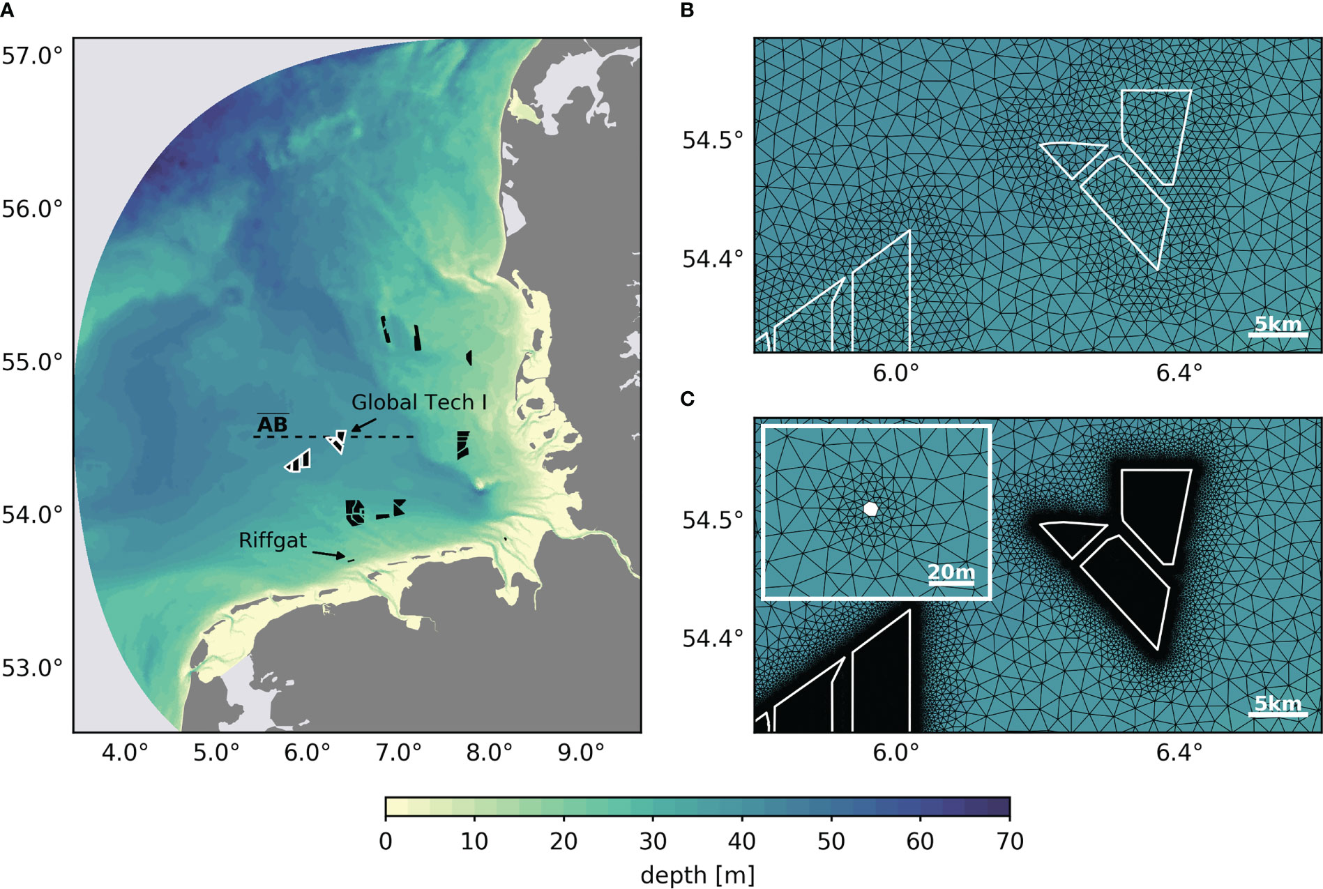
Figure 1 Bathymetry of the German Bight setup (A). Black polygons represent fully commissioned and under construction offshore wind farms in the German Exclusive Economic Zone (status as of November 2021; data obtained from https://www.4coffshore.com/windfarms/). Polygons outlined in white indicate the wind farms shown in (B) and highlighted in Section 3. Dashed black line indicates profile $\overline{\text{AB}}$ (Figure 3). (B) Horizontal grid resolution for the parameterization approach, using a grid size of about 1000 m inside wind farms. (C) Horizontal grid resolution for the dry cell approach around the wind farms (white polygons) and a single monopile (small panel). The wind turbine locations have been obtained from https://www.marktstammdatenregister.de/MaStR.

For the simulations, we utilized the three-dimensional Semi-implicit Cross-scale Hydroscience Integrated System Model (SCHISM, https://github.com/schism-dev/schism), which is a hydrostatic numerical model using Reynolds-averaged Navier-Stokes equations based on the Boussinesq approximation (Zhang et al., 2016). The model domain covers the German Bight region, from the northeastern Dutch coast in the south to the northeastern Danish coast in the north (Figure 1A). Here, our model setup acts as a nested domain within a larger Southern North Sea model introduced by Christiansen et al. (2022a), and was run as a hotstart, meaning that simulations were initialized and controlled at the lateral open boundary by the stored fields from the former North Sea simulations. Thus, a spin-up period was not included.

The new model simulations were conducted for the time period of May to September 2013, to emphasize the effect of structure-induced mixing on the stratification development and to allow comparison to the demonstrated wind wake effects (Christiansen et al., 2022a; Christiansen et al., 2022b). Additionally, longer runs covering the years 2011 to 2015 have been conducted. For the initial state of the new model setup and the open boundary conditions, we obtained sea surface elevation, temperature, salinity, and horizontal velocity from the enveloping Southern North Sea model. Additionally, tidal forcing by eight constituents (M₂, S₂, K₂, N₂, K₁, O₁, Q₁, P₁), daily river discharge, and hourly atmospheric forcing were applied similarly to the governing simulations. A detailed description of the Southern North Sea model setup can be found in Christiansen et al. (Christiansen et al., 2022a; Christiansen et al., 2022b). Note that the wind wake effects from offshore wind farms, which have been studied by Christiansen et al. (Christiansen et al., 2022a), were not included in the sea surface boundary conditions to isolate the effects of turbulent wakes at wind turbine foundations.

The horizontal and vertical grid cell resolution have been adjusted compared to the previous model setup. Here, we used an overall finer horizontal grid resolution, varying between 750 m at the coast and 2000 m in the open ocean, and a finer resolution at offshore wind farm sites of up to 4 m or 250 m, respectively. The final number of horizontal grid cells depended on the wind turbine implementation used. Vertically, the depth-dependent localized sigma coordinates (Zhang et al., 2015) resulted in a maximum of 36 vertical layers in the deep ocean and a minimum of two vertical layers in very shallow waters. The layer thicknesses varied from about 1 m near the sea surface to about 4 m in deep waters, with a layer thickness of 1.5-2 m around the pycnocline. It should be noted here that the depth-dependent number of vertical layers could affect the results of vertical stratification at different wind farm sites due to different vertical resolution of the pycnocline. However, such changes are expected to be minor since the number of layers around the pycnocline varies by a maximum of ±1. The time step of the simulations ranged from 90 s to 120 s, depending on the wind turbine implementation, which is discussed in Section 2.2 and 2.3. Output data is written with an hourly time step.

2.2 Implementation of offshore wind turbine effects

Incorporating the small-scale processes at vertical cylinders into the regional model frame presents a number of numerical challenges. The extreme scale differences of the processes associated with flow past vertical cylinders ($\mathcal{O}$ (10^-3-10⁴) m) make it nearly impossible to capture all flow characteristics with the same modeling approach, and therefore models require certain limitations and assumptions. Here, we focus on the two most prominent approaches used in the recent literature, namely drag parameterization at low resolution (Rennau et al., 2012) and explicit representation of wind turbine foundations at very high resolution (Christie et al., 2012; Cazenave et al., 2016). While these approaches have been able to resemble wake processes, the regional modeling approaches should generally be adopted with care, as the actual processes are still not fully understood (Dorrell et al., 2022) and results are difficult to validate due to a lack of comparable observations and measurements.

Perhaps the greatest challenge in modeling of the small-scale pile effects in regional applications arises from the hydrostatic approximation. For geophysical flows, like ocean currents, the horizontal scales are usually much larger than vertical scales and therefore the latter are typically neglected in the equations of regional models (e.g., Haidvogel and Beckmann, 1998; Cushman-Roisin and Beckers, 2011). Thus, hydrostatic regional modeling is appropriate for mesoscale features and larger dynamics, but becomes limited in the treatment of small-scale non-hydrostatic processes (Haidvogel and Beckmann, 1998), such as wake turbulence at monopiles ($\mathcal{O}$ (10⁰) m), where the use of high grid resolution can cause problems in the model simulations. In addition, the hydrostatic model by definition underrepresents the non-hydrostatic wake turbulence that is expected for highly turbulent wakes at $Re>{10}^5$ in shelf sea waters.

2.2.1 Parameterization of monopile drag and wake turbulence

Structure-induced mixing by subgrid-scale offshore monopile foundations can be accounted for by parameterizing the drag force that a vertical cylinder exerts on the horizontal flow. This approach has long been used in the context of vegetation canopy models (e.g., Wilson and Shaw, 1977; Svensson and Häggkvist, 1990) and has been adopted in previous studies (Rennau et al., 2012; Carpenter et al., 2016; Rivier et al., 2016) to estimate additional anthropogenic mixing from offshore wind turbine foundations. In this method, the drag by a vertical cylinder perpendicular to an unstratified flow can be expressed as

$\begin{array}{ll}{\overrightarrow{F}}_{\mathit{d}}=-\frac{1}{2}{\rho }_0{C}_d{A}_c\left|\overrightarrow{u}\right|\overrightarrow{u}& (2)\end{array}$

where ${\rho }_0$ is the density of the fluid, $C_d$ is the drag coefficient, $A_c$ is the frontal area of the cylinder that is exposed to the free stream, and $\stackrel{\rightharpoonup }{u}$ is the velocity of the free stream (Carpenter et al., 2016), with the negative sign indicating that the drag force is acting in opposite direction of the free stream. Although the parameterization was developed for unstratified flow, Rennau et al. (2012) suggested that the basic principles of the approach also apply for stratified flow under the assumption that momentum transfer between the structure and the flow is independent of stratification.

Here, we consider the pile drag via the model equations. For the implementation into the model equations, the horizontal drag per grid element divided by mass is given by

$\begin{array}{ll}{\overrightarrow{G}}_{\mathit{d}}=-\frac{1}{2}{C}_{d}N\frac{d}{A}\left|\overrightarrow{u}\right|\overrightarrow{u}& (3)\end{array}$

where $d$ is the diameter of the monopile cylinder, $A$ is the horizontal area of the grid cell containing the cylinders, and $N$ is the number of monopiles per grid cell (Rennau et al., 2012). To account for deceleration at grid cells containing offshore wind turbines, the drag parameterization is added to the hydrostatic momentum equation of the SCHISM model, defined as

$\begin{array}{ll}\frac{D\overrightarrow{u}}{Dt}=\frac{\partial }{\partial z}(v\frac{\partial \overrightarrow{u}}{\partial z})-g\nabla \eta +\overrightarrow{F}+{\overrightarrow{G}}_{\mathit{d}}& (4)\end{array}$

with the vertical coordinate represented as $z$, the time $t$, the gravitational acceleration $g$, the horizontal velocity $\stackrel{\rightharpoonup }{u}$, the vertical eddy viscosity $\nu$, the free-surface elevation $\eta$ and $\stackrel{\rightharpoonup }{F}$ as additional forcing terms, such as baroclinic gradient, horizontal viscosity or Coriolis force (Zhang et al., 2016). Note that in SCHISM horizontal velocities are calculated at the sides of grid elements.

In order to account for the production of subgrid-scale wake turbulence, the drag force is also added to the turbulence closure scheme for turbulent kinetic energy and its dissipation (Svensson and Häggkvist, 1990; Rennau et al., 2012; Rivier et al., 2016). Using the generic length-scale model (Umlauf and Burchard, 2003) in SCHISM, the modified turbulent kinetic energy $k$ and dissipation $ϵ$ are calculated as

$\begin{array}{ll}\frac{\partial k}{\partial t}=\frac{\partial }{\partial z}({\nu }_k\frac{\partial k}{\partial z})+P+B-ϵ+P_d& (5)\end{array}$

$\begin{array}{ll}\frac{\partial ϵ}{\partial t}=\frac{\partial }{\partial z}({\nu }_{ϵ}\frac{\partial ϵ}{\partial z})+\frac{ϵ}{k}(c_{1}P+c_{3}B-c_2ϵF_{wall}+c_4{P}_d)& (6)\end{array}$

where ${\nu }_k$ and ${\nu }_{ϵ}$ are vertical turbulent diffusivities, $F_{wall}$ is a wall proximity function, $P$ is the shear production, $B$ is the buoyancy production, and $P_d=-{\stackrel{\rightharpoonup }{G}}_d·\stackrel{\rightharpoonup }{u}$ is the additional production term due to monopile wake turbulence. $c_1$, $c_2$, $c_3$, $c_4$ are model-specific weighting parameters for the dissipation source and sink terms (Umlauf and Burchard, 2003), defined in SCHISM as $c_1=1.44$, $c_2=1.92$ and $c_3=-0.52$ for the $k-ϵ$ model. While Rivier et al. (2016) defined $c_4=c_2$, Rennau et al. (2012) demonstrated the importance of the definition of $c_4$ and its physical implications by showing that mixing efficiency is reduced for $c_4>c_1$ and enhanced for $c_4<c_1$. In this context, Rennau et al. (2012) determined an upper limit value of $c_4=1.75$ and suggested $c_4=0.6$ for strong mixing scenarios and $c_4=1.4$ for weak mixing scenarios.

In general, the results of the drag parameterization are strongly dependent on the choice of scaling parameters in the drag formulation, more precisely the diameter $d$ and the drag coefficient $C_d$, of which the latter has the largest uncertainty. From experimental studies, drag coefficients by a cylinder in an unstratified fluid are expected between $C_d=0.2$ and $C_d=1.3$ (e.g., Shih et al., 1993; Sumer and Fredsøe, 2006), depending on, for example, the turbulence intensity of the approaching stream and the surface roughness. As these conditions can vary by structure, location and flow properties, choosing a fixed drag coefficient may continuously over- or underestimate the frictional processes. Carpenter et al. (2016) showed how different drag conditions influence the results of the drag parameterization. For a low-turbulence scenario ($C_d=0.35$) with tripile foundations and a high-turbulence scenario ($C_d=1.0$) with tripod foundations, structure-induced power removal can differ by a factor of 4.6, demonstrating the uncertainty in structure-induced mixing as a function of structure properties. This uncertainty has to be taken into account when interpreting the results of the canopy-like approach.

2.2.2 Explicit implementation of monopile cylinders

Using unstructured grids, a more intuitive approach is to incorporate monopile foundations as full-depth vertical cylinders into the unstructured horizontal model grid, i.e., as fine-scale islands. This dry cell method requires very high grid resolution around wind turbine locations in order to resolve the small-scale structures, implying a large number of small grid cells around the cylinders, which can create large computational cost. Using the dry cell method in regional unstructured grid models, recent studies (Christie et al., 2012; Cazenave et al., 2016) have been able to resemble downstream wake patterns at offshore wind turbines, looking similar to sediment plume patterns observed by Forster (2018). Nonetheless, the dry cell method is associated to a number of numerical challenges, which will be discussed here.

The limitations of the explicit representation of monopile foundations in the regional model do not arise from the dry cells themselves but from the use of very high resolution that is incompatible with the hydrostatic approximation and the numerical constraints of the regional model. On the one hand, the small grid cells near the wind turbine foundations allow the development of non-hydrostatic vertical circulations that are not accounted for by the hydrostatic model equations, leading to spurious modes in the model simulations. On the other hand, the small grid cells violate the stability criteria of the regional hydrostatic model at an invariant time step, resulting in instabilities and physically unreasonable results.

Here, the semi-implicit SCHISM model uses a combination of implicit and explicit schemes, which results in two constraints for the temporal and spatial discretization: an inverse Courant-Friedrichs-Lewy criterion of CFL ~ $\frac{dt}{dx}>0.4$, and a recommended operating range for the time step between 100-200 s for baroclinic applications (SCHISM v5.7 User Manual). The small grid sizes required by the dry cell approach ($\mathcal{O}$ (10⁰-10¹) m) cannot satisfy both constraints simultaneously and thus result in either numerical instabilities or diffusion due to violation of the CFL criterion or time steps below the recommended range.

Eventually, the dry cell approach leads to spurious modes and numerical noise in small-scale grid cells around the turbines due to numerical or model-specific limitations. These instabilities can be mitigated by using, for example, additional viscosity implementations in the small grid cells, which reduce the spurious modes below the sampling limit of the horizontal resolution by averaging velocities of neighboring grid nodes (Zhang et al., 2016). Previous studies used the Smagorinsky model to control sub-grid scale instabilities (Christie et al., 2012; Cazenave et al., 2016), which appeared to efficiently reduce instabilities in small grid cells. Here, we use the 5-point Shapiro filter implemented in the SCHISM model (Zhang et al., 2016).

2.3 Model simulations

We conducted several simulations to analyze the performance of the approaches and determine the impact of structure-induced mixing by offshore monopiles, while taking into account a recent status of offshore wind farms in the German Exclusive Economic Zone (Figure 1A). The horizontal grid resolution and time step were chosen according to the numerical constraints of each implementation approach. For both approaches, we assumed monopile foundations for simplicity with a diameter of $d$ = 8 m, based on available industry information (Merkur Offshore). Although this may differ from individual wind turbine properties, the assumption of an 8-meter monopile appears appropriate for a generalized impact study, given the many factors that affect the actual foundation drag.

For the parameterization approach, simulations were conducted with a time step of 120 s, similar to the governing Southern North Sea simulation (Christiansen et al., 2022a). To discuss the effects of model parameters, we chose different combinations of pile diameters, drag coefficients, mixing parameters, and grid resolution in each simulation (see Table 1), with values based on earlier studies (Rennau et al., 2012; Carpenter et al., 2016). For the grid resolution, we applied horizontal discretizations of 250 m and 1000 m at wind farm sites, of which the latter results in approximately 78,000 nodes and 152,000 triangles (Figure 1B). All wind farms depicted in Figure 1A are considered in the parameterization approach.

TABLE 1

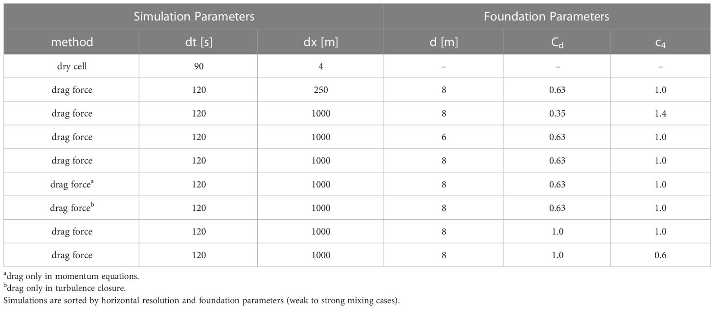
Table 1 List of conducted model simulations involving wind turbine implementations.

The dry cell approach requires a tradeoff between process accuracy, numerical stability, and computational efficiency, due to its limitations. Although numerical instabilities are inevitable for this approach, we aimed to moderate the numerical noise by using coarser resolution than previous studies that used 2.5 m resolution or lower at the monopile foundations (Christie et al., 2012; Cazenave et al., 2016). Here, we chose a grid resolution of about 4 m around the cylinders, almost linearly increasing to about 1000 m over a five-kilometer radius of the wind turbines (Figure 1C), which increases the size of adjacent grid cells and thus decreases numerical instabilities. In addition, we applied the Shapiro filter with a maximum damping factor of 0.5 and in five-fold iteration. In order to reduce the computational cost and allow seasonal simulations, we reduced the number of wind farms to six, which are all located in seasonally stratified deep waters of the German Bight (see Figure 1C). Still, the setup results in approximately 1.4 million nodes and 2.8 million triangles. Simulations were conducted with a time step of 90 s to relax the stability criterion violations in small grid cells. This time step falls already just below the recommended operating range for the baroclinic application, but the simulations still produce reasonable results.

For the analysis, simulations including the wind turbine effects (OWF) are compared to reference simulations without the parameterized wind turbine effects (REF) by showing instantaneous or time-averaged differences (OWF-REF) over the simulation period between May to September. Both OWF and REF were calculated for each grid configuration and compared accordingly. For time-averaged vector quantities, like velocities, we distinguish between the differences of the absolute values of the velocity $\Delta u_{abs}$ (change in current speed) and the differences of the velocity vector $\Delta u$ (change in current velocity):

$\begin{array}{ll}\Delta u_{abs}= \langle \left|{\overrightarrow{u}}_{\mathit{OWF}}\right|\rangle - \langle \left|{\overrightarrow{u}}_{\mathit{REF}}\right|\rangle ,\Delta u=\langle {\overrightarrow{u}}_{\mathit{OWF}}\rangle -\langle {\overrightarrow{u}}_{\mathit{REF}}\rangle & (7)\end{array}$

where $\langle \rangle$ indicates the temporal mean and $| |$ the absolute value of the velocity vector $\overrightarrow{u}=(u,v)$.

3 Results and discussion

3.1 Validation of wind turbine implementations

Both the flow resistance of the dry cells and the parameterized monopile drag affect the hydrodynamics in adjacent grid cells of offshore wind turbines. The main difference lies in the physical representation of the downstream wake structures related to the choice of horizontal grid resolution, which is discussed in this section. In fact, the comparison elucidates the impact of high and low resolution in hydrostatic regional modeling, while showing the consequences in relation to structure-induced mixing by offshore wind turbine foundations.

The small-scale vertical structures in the dry cell approach deflect the local horizontal flow and generate distinct wake patterns downstream of the wind turbines (Figure 2A). The wakes extend well downstream of the monopiles with an average length of about 600 m (Supplementary Figure 1) and are consistent with recent sediment plume observations by Vanhellemont and Ruddick (2014) and Forster (2018). Here, wake lengths exceed the spacing distance between neighboring wind turbines and affect upstream flow conditions. Compared to the upstream velocity, the depth-averaged downstream velocity is reduced by about 0.11 m/s on average at a distance of 10 m behind the monopiles and by about 0.01-0.02 m/s at a distance of 50-100 m downstream (Supplementary Figure 1B). These values are in agreement with the surface velocity anomalies of about 0.05 m/s simulated by Cazenave et al. (2016). In the hydrostatic simulation, the drag of the monopile is balanced by the changes in surface displacement around the pile. Thus, we can estimate the simulated drag coefficients in the dry cell approach by equating the drag force (Equation (2)) with the hydrostatic pressure force acting on the vertical cylinder $({\overrightarrow{u}}_{\mathrm{OWF}}=\sum _i{p}_i{\overrightarrow{n}}_{i}d{A}_i)$, resulting in an average drag coefficient of about $C_d=0.27$. This value is within a reasonable range of drag coefficients experimentally found for smooth cylinders in a non-turbulent free stream at $Re>{10}^6$ (Shih et al., 1993; Sumer and Fredsøe, 2006). However, since in the tidal environment the free stream contains turbulence and monopiles are unlikely smooth in reality, the drag coefficient is expected more than twice the estimated value (see, e.g., Achenbach, 1971) and is therefore insufficiently simulated by the hydrostatic dry cell approach.

FIGURE 2

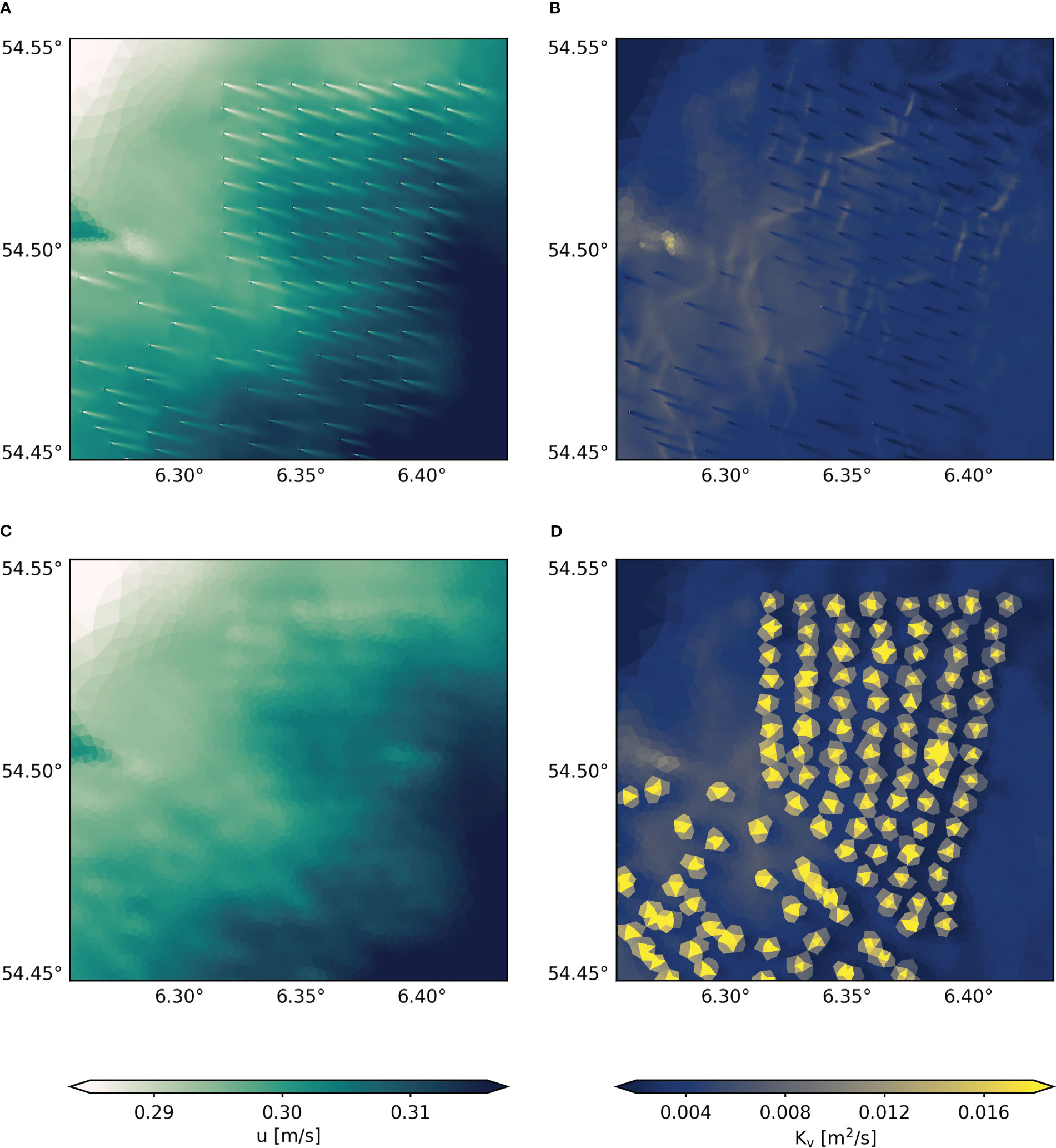
Figure 2 Snapshot of the simulated wake effects at Global Tech I for depth-averaged horizontal velocity u (A, C) and depth-averaged vertical eddy diffusivity K_v (B, D) on May 1. Top panel show wake patterns for the dry cell approach (A, B), bottom panels show wake effects for the parameterization approach ($C_d$ = 0.63 and $c_4$ = 1.0) at 1000 m resolution (C, D).

For the dry cell approach, we used five-fold iteration of the Shapiro filter and a resolution of 4 m at monopiles to mitigate numerical noise. Parameter tests show that the application of a viscosity-like filter is necessary to obtain appropriate wake structures and to avoid severe numerical instabilities and non-hydrostatic modes due to high resolution, which otherwise superimpose the actual wake patterns (see Supplementary Figure 2A). However, not only instabilities but also the wakes are sensitive to the filtering, as the Shapiro filter adds artificial viscosity to the small grid cells and thus affects the dynamic properties of the horizontal flow. In the present case, for example, a twenty-fold iteration of the Shapiro filter would result in shorter and broader downstream wake structures (see Supplementary Figure 2C), affecting the drag processes at the monopiles.

The fine grid resolution in the hydrostatic regional model requires an arbitrary degree of numerical tuning while producing insufficient wake patterns that become sensitive to the numerical parameters chosen. This drawback is emphasized by the associated patterns in the vertical eddy diffusivity, a measure for vertical mixing rates. Unlike the reality shown in laboratory experiments (e.g., Williamson, 1996), the hydrostatic dry cell approach does not produce additional turbulent mixing along the wakes, because non-hydrostatic wake turbulence cannot be simulated by the hydrostatic model. Without a proper parameterization addressing this deficiency, mixing rates downstream of the monopiles even decrease (Figure 2B). This diffusivity reduction is related to the reduction of the vertical shear inside the wakes and the lack of horizontal shear production in the turbulence closure equations (Equations (5), (6)), which in reality increases at the edges of the narrow wake structures. Consequently, structure-induced mixing is significantly underrepresented in the hydrostatic dry cell approach, which will bias the effects on density stratification and turbulent mixing. Thus, as also noted by van Berkel et al. (2020), regional implementation of the dry cell approach without additional mixing parameterization (such as inclusion of horizontal shear production) should be interpreted with caution.

The parameterization approach, on the other hand, allows for low resolution at wind farm sites and thus avoids numerical instabilities or contradictions with the hydrostatic approximation. At scales on the order of 10² m, wake processes at wind farm can be considered hydrostatic and additional turbulence from non-hydrostatic sub-grid scale processes can be assigned through the drag equation. Consequently, the parameterization approach can be considered reliable in terms of the wake turbulence impacts, despite not resolving the actual wakes themselves. Nonetheless, uncertainties can arise from site-specific model parameters, like the drag coefficient, which determine the simulated wake magnitudes. Here, the initial values for the drag coefficient $C_d$ and the mixing parameter $c_4$ are based on Rennau et al. (2012), assuming moderate mixing with $C_d=0.63$ and $c_4=1.0$. In addition, we start by using a grid resolution of about 250 m inside wind farms for illustration of the momentum extraction and additional wake turbulence at monopile grid cells. Note that this horizontal discretization is slightly below the lower limit of the CFL criterion (300 m) and might bias the magnitudes. The parameterization method generates generally weaker, indistinct velocity anomalies at wind turbines sites due to consideration of larger grid cells (Figure 2C). Here, the depth-averaged horizontal velocity decreases by about 0.01 m/s compared to adjacent grid cells.

In terms of turbulent mixing, the SCHISM model limits the advantages of the parameterization approach, as the $k-ϵ$ equations do not account for the advection of turbulence and therefore structure-induced mixing cannot be transported downstream. As a result, additional vertical diffusivity develops locally at the predefined wind turbine elements (Figure 2D). Since wakes have been shown to extend much further than 250 m (Vanhellemont and Ruddick, 2014; Forster, 2018; Schultze et al., 2020), the small grid cells might underrepresent the turbulent mixing inside offshore wind farms. However, Schultze et al. (2020) have shown that the wake turbulence is confined to the near field of monopiles (~200 m). Here, we propose a horizontal resolution of about 1000 m, covering the observations of both Forster (2018) and Schultze et al. (2020), and accounting for potential advection of turbulence. The impact of the horizontal grid resolution inside wind farms will be discussed in Section 3.2.

For the impact assessment, validation of the additional structure-induced mixing inside the model is necessary. To date, however, there are few in-situ measurements of foundation wake structures within offshore wind farms, especially in stratified waters (Floeter et al., 2017; Schultze et al., 2020). Following the observation period given in Floeter et al. (2017), we analyze here the changes in summer stratification and compare them with the in-situ observations. Note that at the time of the measurements by Floeter et al. (2017) fewer wind farms were installed and structure parameters may have been different than in the model simulations. Figure 3 shows the mean stratification strength, described by the potential energy anomaly, in July 2013 in the region of the Global Tech I wind farm. Here, the wind farms are located near the frontal regions and therefore stratification in the region naturally decreases from northwest to southeast, with a spatial variability of about 10-15 J/m³ without wind farm effects.

FIGURE 3

Figure 3 Mean potential energy anomaly Φ in July 2013 for the parameterization approach at 1000 m resolution (A) and the dry cell approach (B). White polygons represent offshore wind farms, black dashed line indicates the course of profile $\overline{\text{AB}}$. (C) Potential energy anomaly Φ along profile $\overline{\text{AB}}$ for different scenarios of the parameterization and dry cell approach. White sector indicates the intersected wind farm sites. Dashed white lines indicate limits of map frame in (A, B). (D) Relative changes in potential energy anomaly ΔΦ for the drag parameterization approach. Gray vertical bars show estimated changes in potential energy anomaly using $C_d$ = 0.35, $C_d$ = 0.63, $C_d$ = 1.0 (left to right).

The parameterization and dry cell approach exhibit significant differences in terms of additional mixing and associated stratification anomalies near the offshore wind farms (Figures 3A-C). For a moderate mixing case using $C_d=0.63$ and $c_4=1.0$ (see Table 1), the parameterization approach (1000 m resolution) produces small anomalies in the monthly-mean potential energy, with reductions of about 5-10 J/m³ compared to surrounding areas (Figures 3A, C). These magnitudes are within the spatial variability and also natural annual and interannual variabilities, but are comparable to the observations of Floeter et al. (2017). In contrast, the dry cell approach exhibits extensive reductions in potential energy anomaly of more than 20-50 J/m³ at wind farm sites, which extend far from the associated wind farm locations (Figures 3B, C). In fact, monthly-mean potential energy anomaly decreases to below 10 J/m³ within wind farms, implying a nearly well-mixed water column in the stratified region due to monopile drag.

To help verify the simulated stratification changes, we use a theoretical mixing model derived by Carpenter et al. (2016) as additional reference. The model estimates structure-induced changes in stratification by offshore wind farms based on the time a water parcel spends inside a wind farm, the power removed by the structure from the flow, and the pycnocline thickness at the wind farm site. Here, we use Equation (3) to calculate the power dissipation by wake turbulence per unit area, estimate the thermocline thickness using a threshold of vertical temperature difference of 0.2°C (Boyer Montégut et al., 2004), and calculate residence times through the monthly-mean current velocity and the size of the Global Tech I wind farm. Using different values for the drag coefficient and an estimated thermocline thickness of 9 m, the theoretical reductions in monthly-mean potential energy anomaly at Global Tech I agree well with the simulated changes here (Figure 3D). For $C_d=0.63$, for example, the theoretical reduction can be calculated as about 3.6 J/m³. However, there remains an uncertainty about these estimates as the simulated thermocline might be too diffusive (Luneva et al., 2019) and the mixing at Global Tech I is influenced by neighboring wind farms. Furthermore, calculated stratification changes between 1-5 J/m³ are within the uncertainty of the drag coefficient (Figures 3C, D). Nonetheless, the parameterization approach produces similar results to the observations of Floeter et al. (2017), and both the simulations and the observations are in agreement with the theoretical estimates, suggesting that the physics are similarly captured and that the parameterization approach produces reasonable results.

The stratification profiles for the dry cell approach, on the other hand, illustrate the problems associated with the hydrostatic approximation and numerical instabilities (Figure 3C). The changes in monthly-mean potential energy anomaly deviate strongly from both the theoretical estimates and the in-situ observations. Adjustments of the Shapiro filter can reduce these effects originating from the wind farms (see Supplementary Figures 2D-F), but even with twenty-fold filter iteration, the stratification anomalies are still much stronger compared to the other results. More importantly, same effects occur for a similar high-resolution grid configuration but without dry cells at monopile locations (Figure 3C), showing that the problems arise from the horizontal resolution and not from the dry cells themselves. This emphasizes the problematic use of small grid cells with hydrostatic approximation and makes the dry cell approach unsuitable for hydrostatic regional modeling without significant modification. These problems, however, are model specific and might be avoidable by using non-hydrostatic modeling, e.g., FVCOM-NH (Lai et al., 2010) or Thetis-NH (Pan et al., 2020). For hydrostatic models such as the SCHISM model, we propose the use of parameterization methods to investigate the mixing effects from offshore wind turbine foundations, and this approach is followed henceforth.

3.2 Local impact of structure-induced mixing

To understand the regional impact of flow disturbance and mixing from offshore wind farms, we start by examining the local processes at wind farm sites. For this purpose, we separate the processes of momentum extraction and turbulence production to determine their individual impacts on the hydrodynamics using. For the process separation, we performed individual simulations in which the drag term (Equation (3)) was considered in either the momentum equation (Equation (4)) or the turbulence closure scheme (Equations (5), (6)), but not both. In these simulations, the horizontal resolution inside wind farms was kept at 1000 m. In addition, we used previous experiments with higher resolution (250 m) and lower resolution (1000 m) at wind farm sites to assess the effects of the horizontal spatial discretization. The associated hydrodynamic changes averaged over the first month of simulation (May 2013) are depicted in Figure 4.

FIGURE 4

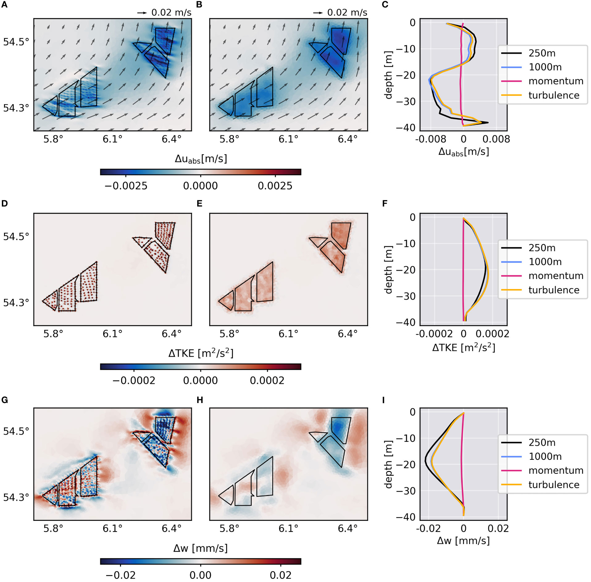
Figure 4 Monthly-mean changes due to monopile drag after the first month of simulation (May 2013) in horizontal current speed u_abs (A-C), turbulent kinetic energy TKE (D-F) and vertical velocity w (G-I). Horizontal patterns are depicted for 250 m resolution (left) and 1000 m resolution (right). Gray arrows show the mean flow direction of the reference simulation. Black polygons indicate wind farms. Vertical profiles show changes averaged over Global Tech I for the full drag parameterization (Equation (3)) at different resolutions and for the differentiated momentum extraction (Equation (4)) and turbulence production (Equations (5), (6)) at 1000 m resolution.

Because of the local monopile drag, the magnitudes of the horizontal velocity decrease at wind farm sites, causing horizontal gradients in the surrounding current speed and affecting downstream currents (Figures 4A, B). The monthly mean changes in the depth-averaged current speed ($\Delta u_{abs}$) are about 0.001-0.003 m/s, which is about 1% of the simulated local averaged tidal current speeds in May (0.3 m/s) and about 10% of the monthly mean flow velocity (0.01-0.03 m/s). Note that strong instantaneous tidal currents can cause larger magnitudes than appear in the monthly average because the drag force scales quadratically with the current velocity (Equation (3)). Unlike the depth-averaged current speed, the vertical current speed profile averaged over Global Tech I is more notably affected by the structure-induced drag (Figure 4C). In fact, the local drag causes negative and positive changes of up to -0.008 m/s and +0.004 m/s, respectively. Here, Figure 4C shows that the alteration in the vertical current speed profile is essentially related to the enhanced mixing due to the structure-induced turbulence. While the momentum extraction causes minor reductions in the averaged current speed (0.0005 m/s), the additional turbulence alters the vertical profile with much greater magnitude and similar to the combined effect of momentum and turbulence. Consequently, the amplitude variations over depth are related to additional turbulence, which is discussed later in Section 3.3.

The increase in monthly mean turbulent kinetic energy (TKE) averaged over depth at offshore wind farm sites is shown in Figures 4D, E. Due to missing advection terms in turbulence closure scheme (Equations (5), (6)), the additional turbulence occurs only in the grid cells connected to the monopile locations. However, averaged over the wind farm area, the vertical profiles show that both grid resolutions result in similar increases in monthly mean TKE (Figure 4F), proving that the grid scaling factor in the drag equation (Equation (3)) is preserving the monopile drag at lower resolution. The profiles also show that the change in TKE is solely related to the direct turbulence parameterization, while the indirect effect of momentum extraction has essentially no effect.

As the monopile drag alters local current speeds and turbulence, the local changes trigger vertical velocities, which result in upwelling and downwelling patterns at wind farm sites in the monthly mean (Figures 4G, H). Again, the additional turbulence productions acts as the dominating factor in the structure-induced changes. The monthly-mean changes in depth-averaged vertical velocity are about 0.01-0.02 mm/s and thus around 1 m/day. At Global Tech I, the monthly-mean vertical velocity decreases inside the wind farm and increases at the sides of the wind farm relative to the mean flow direction (Figures 4G-I). The patterns in vertical velocity suggest blockage of the mean horizontal currents and resemble observations of Floeter et al. (2017) at Global Tech I. Floeter et al. (2017) suggested the blocking effects as a result of increased vertical mixing within the wind farms, similar to the island stirring effect by Simpson et al. (1982), with the increased mixing inside the wind farms leading to destratification and local upwelling. Indeed, the simulated effects here agree well with the assumptions by Floeter et al. (2017), however, the local upwelling relative to the mean flow direction does not occur consistently at the other wind farms. This is related to changing tidal current directions, which relocate the upwelling/downwelling patterns over time and hinder the occurrence of distinct patterns in the monthly means.

Figure 4 shows that generally smaller grid cells increase the variability at wind farms and resolve processes in between the monopiles. Nevertheless, the higher resolution does not seem to affect the large-scale effects in the vicinity of the wind farms. Thus, higher resolution at wind farm sites does not appear to add significant value to the regional effects of structure-induced mixing, supporting the use of the coarse-resolution parameterization approach. Instead, high resolution is most relevant in the local analysis of wake effects within of offshore wind farms. Here, however, the local analysis is limited by the CFL criterion.

Turbulent mixing appears to be the most dominant consequence of the monopile drag, implying implications for local stratification in the seasonally-stratified waters of the German Bight. Vertical profiles of water temperature and vertical eddy diffusivity, averaged over the summer months of June through August, and the respective evolution of seasonal stratification are shown in Figure 5 for two different wind farm locations. The two examples correspond to the Global Tech I wind farm, located in seasonally stratified deeper waters, and the smaller Riffgat wind farm, located in unstratified waters northwest of the East Frisian island of Borkum. At Global Tech I, summer stratification is strong with a mean temperature change of more than 3°C across a pycnocline thickness of about 9 m (Figure 5A). Here, mixing predominantly occurs in the surface and bottom mixed layers, and decreases in the pycnocline (Figure 5B). Stratification strength reaches a maximum at the end of July with more than 80 J/m³ in magnitude (Figure 5C). In contrast, the temperature gradient at Riffgat is small. Here, the mean temperature difference from top to bottom is less than 0.3°C during summer (Figure 5D) and the potential energy anomaly does not exceed 6 J/m³ (Figure 5F). As a result, the vertical mixing rate is significantly stronger than at Global Tech I, with the most pronounced mixing occurring in the middle of the water column (Figure 5E).

FIGURE 5

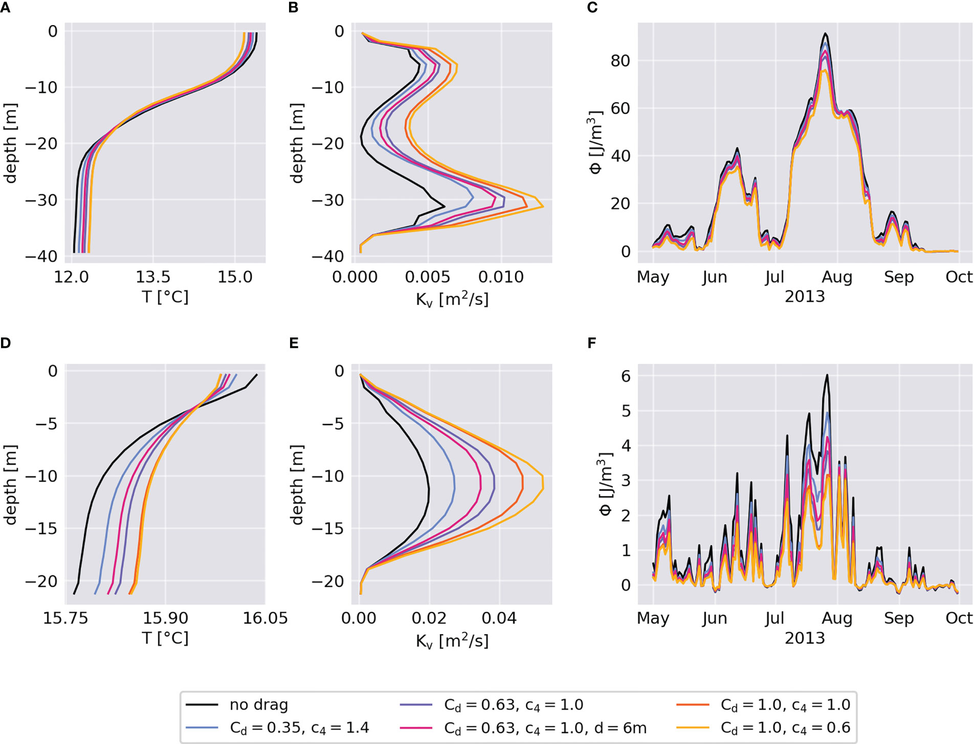
Figure 5 Vertical changes in temperature T (A, D) and vertical eddy diffusivity K_v (B, E) averaged between June and August, and temporal changes in potential energy anomaly Φ (C, F) from May to October, each for different scenarios of the parameterization approach. The upper panels show changes in stratified waters averaged over the Global Tech I wind farm and the lower panels show changes in nearly-unstratified waters averaged over the Riffgat wind farm.

Despite different stratification conditions, the processes at the two wind farms act similar with respect to temperature and diffusivity changes. In consequence of the additional structure-induced turbulence, the mean temperature gradients at wind farm sites decrease and mean vertical diffusivities increase (Figure 5). The magnitudes of the perturbations depend strongly on the scaling parameters used in the simulations as well as on local conditions. For instance, mean vertical diffusivity increases by about 25% for a low turbulence scenario ($C_d=0.35$, $c_4=1.4$), but by about 100% for the scenario of very strong turbulence ($C_d=1.0$, $c_4=0.6$), indicating a strong uncertainty about the amount of additional mixing at individual wind farms. Here, the parameters of the drag equation ($C_d$ and $d$) significantly affect both the changes in stratification and the turbulent mixing rates, whereas the parameter $c_4$ appears to determine mainly the latter. The uncertainty caused by the drag parameters has been mentioned in earlier studies (Carpenter et al., 2016; Dorrell et al., 2022) and must be taken into account for the application of the parameterization approach and the interpretation of the simulation results. Nevertheless, using moderate values for the scaling parameters, e.g. $C_d=0.63$ and $c_4=1.0$, seems to provide sufficient results for the regional impact, though effects might be under- or overestimated in some regions.

Regardless of stratification conditions, the additional mixing by monopiles alters and, in particular, reduces the potential energy anomaly inside offshore wind farms (Figures 5C, F). If the water column is stable ($\varphi >0$), the magnitudes of these changes varies between 0-15 J/m³ and account for more than 10-50% of the actual potential energy anomaly. In this context, the changes are stronger in stratified waters, as here the turbulence has a bigger potential to disturb the vertical density distribution and affect the stability of the water column. However, percentage changes are more pronounced for weaker stratification. The stratification changes are in general more than twice as strong for high turbulence cases than for low turbulence cases, indicating again the uncertainty due to drag conditions.

3.3 Regional impact of structure-induced mixing

The impact of structure-induced mixing on the hydrodynamic conditions is found to extend well beyond the offshore wind farm sites, as also shown by Rennau et al. (2012) for a case study in the Baltic Sea. This includes advection of disturbances into the far field of offshore wind farms or larger scale structural changes due to perturbations of mesoscale circulation and baroclinic flows. Here, we focus on the extraction of horizontal momentum, the generation of turbulent mixing, and the implications for the stratification. Figure 6 shows the changes in the hydrodynamic parameters averaged over the simulation period from May to September.

FIGURE 6

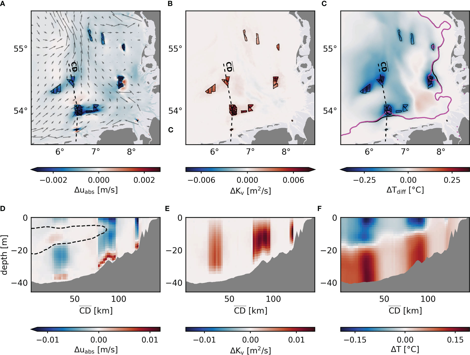
Figure 6 Changes in depth-averaged current speed u_abs (A), depth-averaged vertical eddy diffusivity K_v (B) and vertical temperature differentials T_diff (C) averaged between May and September for the parameterization approach. Gray arrows in (A) show the mean flow direction of the reference simulation. Solid magenta and black lines in (C) indicate the mean frontal positions in OWF and REF, respectively. Dashed black lines indicate profile $\overline{\text{CD}}$, black polygons indicate wind farms. Respective changes in current speed, eddy diffusivity and temperature averaged between May and September along profile $\overline{\text{CD}}$ are depicted in (D-F). Dashed black line in (D) indicates pycnocline estimates, based on the buoyancy frequency N² ≥ 5 x 10^-4 s^-1 (see Dorrell et al., 2022).

The structure drag reduces the depth-averaged current speeds within offshore wind farms and influences respective downstream currents along the prevailing flow direction. Although the reductions thereby originate at wind farm sites, the simulations show that the averaged current speed ($u_{abs}$) decreases widely over the entire German Bight area (Figure 6A). This includes changes advecting along the predominant downstream directions, as well as a general reduction in current speed of about 0.0005 m/s along the German coast. The most pronounced changes occur at wind farm sites with average magnitudes of 0.001-0.002 m/s, and especially at large wind farms and clusters with high turbine density, where magnitudes can exceed 0.003 m/s. These changes are again minor compared to the simulated average tidal current speeds in the German Bight (0.20-0.40 m/s), but account for 10% of the simulated mean currents (0.02-0.03 m/s) and extend significantly on a spatial scale. The structure-induced changes exhibit magnitudes in the same order as the alterations due to wind stress reduction from wind wakes (Christiansen et al., 2022a; Christiansen et al., 2022b), suggesting that the ultimate impact by offshore wind farms on the marine environment will be a complex interaction of atmospheric and hydrodynamic effects.

Figure 6D shows a vertical cross section through different wind farm clusters from deep stratified waters to shallow mixed waters. The induced speed changes over depth are again about one order of magnitude larger than those in the depth average, with more than 0.01 m/s and thus up to 5% of the average tidal current speed. While structure-induced mixing is the main factor driving the current speed changes (as seen in Figure 4C), it becomes evident here that the amplitudes of the changes are related to vertical density gradients and mixing rates in the water column (Figure 6D). The increased turbulence induced by monopile drag penetrates areas of lower mixing rates, such as the pycnocline or bottom boundary layer, where stronger vertical current shear is expected (see Dorrell et al., 2022). Induced turbulent mixing makes the density and horizontal velocity more vertically diffused and uniform, leading to positive anomalies in areas with strong vertical gradients and negative anomalies elsewhere (Figure 6D). Thereby, the positive anomalies within the pycnocline disappear as stratification declines toward the well-mixed shallower waters, and occur solely within the bottom boundary layer.

While affecting other parameters like currents and density far from the monopiles, structure-induced mixing increases turbulence and vertical mixing rates mainly at wind farm sites (Figure 6B). Since wake turbulence has been shown to be confined to the near field of the narrow monopile wakes (Schultze et al., 2020), these localized changes in turbulence and mixing rates appear consistent with the observations. Here, the changes in mean vertical diffusivity are up to twice as strong as the actual mean vertical diffusivity, particularly in less turbulent, stratified waters. The magnitudes increase towards the shallower waters (Figure 6E), where tidal velocities are generally stronger and thus enhance the velocity-dependent turbulence production. The increase in additional mixing towards the coast is also reflected in changes in horizontal current speed (Figure 6D). Compared to wind wake effects (Christiansen et al., 2022a; Christiansen et al., 2022b), the local mixing by monopiles is significantly stronger by at least one order of magnitude, suggesting that structure-induced mixing will dominate the wind-driven effects at wind farm sites. However, note that these numbers are based on arbitrary choices of $c_4$, which needs to be tuned in future studies based on process studies of turbulent wakes, e.g., Schultze et al. (2020).

The additional turbulent mixing from monopile drag influences the vertical density distribution and thus seasonal stratification development. Although the structure-induced mixing is confined at the wind farm sites (Figures 6B, E), mixed water conditions can be detected across the entire German Bight (Figures 6C, F). Mixing reduces the averaged vertical temperature differential from the surface to the bottom layer by about 0.1-0.2°C, with the strongest reduction in stratification of more than 0.3°C occurring at wind farm sites (Figure 6C). These changes account for up to 50% of the simulated mean stratification between May to September. Strong mixing at densely built wind farms near tidal mixing fronts can even shift the mean frontal position to deeper waters as the vertical temperature stratification collapses (Figure 6C).

In stratified months, the structure-induced mixing transports colder water from the bottom layers to the surface and warm surface water into deeper layers (Figure 6F), reducing the vertical temperature gradient at wind farm sites, as also seen for the temperature profiles at the Global Tech I wind farm (Figure 5A). In this process, the vertical boundary between temperature reductions and increases follows the course of the thermocline here. The changes in mean temperature at wind farms reach up to ±0.2°C in stratified waters, and thus up to 20% of the interannual variability of sea surface and bottom temperatures in the southern North Sea (Daewel and Schrum, 2017). Here, the mean sea surface cooling between May and September is up to five times stronger than the mean sea surface warming that occurs in the context of atmospheric wind wake effects (Christiansen et al., 2022a), and thus likely superimposes the latter when looking at the cumulative offshore wind farm effect.

The regional effects of structure drag are sensitive to hydrodynamic conditions, such as horizontal advection, baroclinic conditions or the stratification, which may vary over time, e.g., seasonally or annually. Thus, it becomes important with regard to the impact assessment to distinguish temporal signals from persistent changes in the local dynamics. For this reason, we conducted additional long-term simulations of the monopile effects, covering the years 2011 to 2015. The long-term simulations were conducted using the parameterization approach with 1000 m resolution at wind farm sites, $C_d=0.63$ and $c_4=1.0$.

Changes in five-year mean depth-averaged horizontal velocity ($\Delta u$) show a distinct reduction in residual currents near offshore wind farms, which extend far downstream along the predominant northward circulation (Figure 7A). Note that mainly the magnitude of the flow velocity is affected here, while the basic flow direction essentially remains. The monopile drag influences the surrounding dynamics, resulting in an attenuation of the current velocity in the center of the German Bight, where the wind farms are located, and an increase in the current velocity along the coast and especially the northeastern part of the Dogger Bank (55°N, 5°E). The mean horizontal velocity changes by about ±1 mm/s on average and up to ±4 mm/s at wind farm sites, accounting for about ±5-15% of the local current velocities (Figure 7A). These alterations are on a similar order of magnitude to the annual and interannual variabilities in the southern North Sea (Daewel and Schrum, 2017), and thus can be substantial to associated velocity-dependent biogeochemical processes such as sedimentation or larval dispersal (van Berkel et al., 2020). Increasing offshore wind development in the German Bight could result in large-scale blocking effects and deflection of coastal circulation towards central North Sea areas, where horizontal current velocities increase. The reductions in mean current velocity may create positive feedback on mixing processes by increasing the time as water parcel spends inside the wind farm area. At Global Tech I, for example, mean velocity decreases by 6.4% of the mean current, which results in a 6.8% longer residence time ${\tau }_{adv}$ at Global Tech I, using ${\tau }_{adv}=L/\overline{u}$ and $L=8$ km from Carpenter et al. (2016). This, in turn, could lead to a 6.8% greater reduction in stratification than if current reductions were not considered.

FIGURE 7

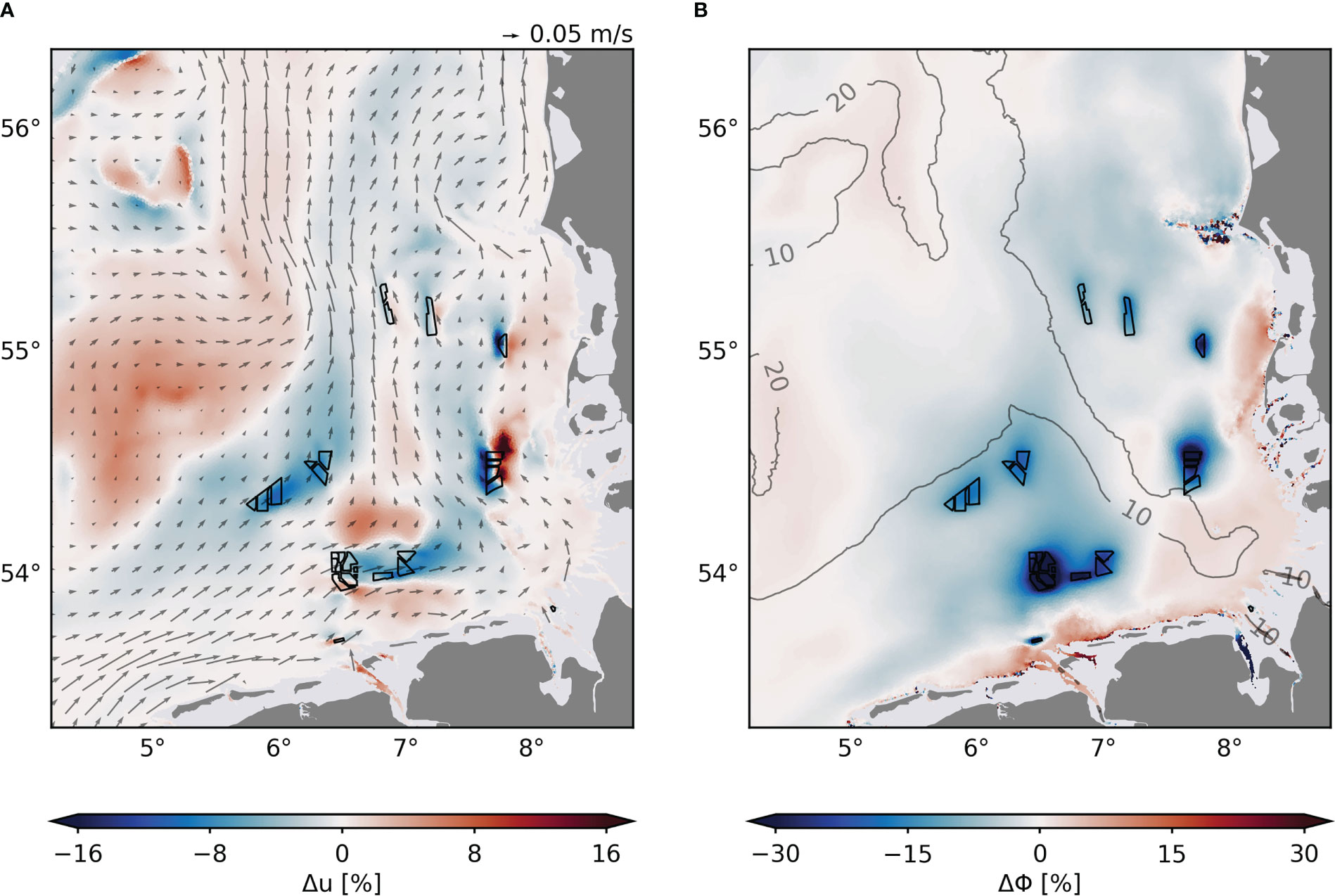
Figure 7 Long-term percentage changes in depth-averaged horizontal velocity u (A) and potential energy anomaly Φ (B) averaged over the years 2011-2015. Gray arrows indicate direction of mean residual velocity in (A), contour lines indicate mean potential energy anomaly [J/m³] in (B). Black polygons indicate wind farms. Water depths below 5 m are masked.

The structure-induced mixing changes the stratification conditions in the German Bight. On the five-year average the potential energy anomaly decreases by 10-15% at wind farm sites, at which maximum values of more than 30% reduction emerge at wind farms in shallower waters near the tidal mixing fronts (Figure 7B). The advection of mixed water masses distributes the anomalies along the northward circulation, reducing the area-wide stratification by about 5%. These effects are accompanied by an increase in potential energy anomaly of about 5% along the shallow German coast and about 1% near the Dogger Bank area. Although the strongest changes in potential energy anomaly occur in stratified waters during the summer periods (Figures 5C, F), we also see that the mixing changes the potential energy anomaly in mixed and unstable waters, where the percentage changes become most substantial. However, note that averaging over winter conditions may bias the annual mean changes at seasonally stratified wind farms, where stratification can decrease by up to 15 J/m³ during the summer.

In general, the long-term changes in stratification have the potential to influence the ecosystem dynamics in areas occupied by offshore wind infrastructure. Stratification provides a natural barrier for vertical exchange of nutrients, oxygen or phytoplankton in the water column and significantly determines the seasonal shelf sea productivity (Simpson and Sharples, 2012; van Leeuwen et al., 2015). Anthropogenic mixing from offshore wind turbine foundations will translate to local biogeochemical processes such as nutrient dynamics and light availability in surface layers (Floeter et al., 2017; Dorrell et al., 2022) or oxygen concentration in deeper layers (Daewel et al., 2022; Dorrell et al., 2022), with consequences for local and regional ecoystem productivity. In the German Bight, primary and secondary production is confined by the frontal position to permanently mixed and intermittently stratified waters (Daewel and Schrum, 2013). Here, additional mixing and shifting of tidal mixing fronts could expand the production to deeper waters and increase the ecosystem productivity in the German Bight. In addition, potential larval survival, which is sensitive to temperature and surface layer mixing (Daewel et al., 2015), could be affected by the changes in stratification. Ultimately, alterations in ecosystem productivity could cascade to higher trophic levels, such as fish or sea bird populations, which adapt to phythoplankton growth (Dorrell et al., 2022). For instance, diver birds have been suggested to adapt to frontal positions in the area of the German Bight (Skov and Prins, 2001).

Future offshore wind scenarios are likely to amplify the impact on hydrodynamics and could fundamentally change stratification conditions and associated ecosystem dynamics in the German Bight, indicating the need for further investigation on the hydrodynamic and biogeochemical consequences of structure-induced mixing. This includes interaction with atmospheric wake effects and determination of the cumulative offshore wind farm impacts. Daewel et al. (2022) demonstrated large-scale consequences of surface wind speed reduction from offshore wind farms on biogeochemistry, including spatial redistributions of annual primary production and bottom oxygen concentrations. The interaction of both wind farm effects, however, is expected very complex and dependent on environmental conditions. Changes in horizontal currents and surface layer mixing from wind speed reductions (see Christiansen et al., 2022a; Christiansen et al., 2022b) could partly amplify or compensate for the velocity anomalies and turbulent mixing from monopile drag and influence the total impact on ocean physics and ecosystem dynamics. Nonetheless, anthropogenic mixing is expected dominant at offshore wind farm sites.

4 Conclusion

With increasing offshore wind energy development in coastal seas, investigations of the consequences for the marine environment are becoming increasingly important. Here, we presented two methods of simulating the effects of structure-induced mixing by offshore wind turbine foundations at the scale of regional numerical models and discussed the improper use of high resolution with the hydrostatic approximation. We show that the dry cell method encounters numerical problems and produces insufficient wake patterns, since the dynamics resolved at very high resolution do not satisfy the hydrostatic approximation and further parameterizations must be added to simulate small-scale processes. In contrast, the parameterization approach appears as a suitable method to account for subgrid-scale wake turbulence. We conclude that for assessing the large-scale impacts of structure-induced mixing it is more reasonable to use low-resolution parameterizations ($\mathcal{O}$ (10²-10³) m) supported by high-resolution non-hydrostatic modeling ($\mathcal{O}$ (≤10¹) m), e.g., Large Eddy Simulations as in Schultze et al. (2020), which can be used to analyze small-scale wake processes and upscale the effects for regional models.

Using the drag parameterization, our results show that monopile drag not only influences the local hydrodynamic conditions at offshore wind farms, but also the conditions in the far field of the wind turbine arrays. Here, additional wake turbulence and associated turbulent mixing represent the main drivers of the structure-induced processes. Mean horizontal currents and density stratification can change locally by about 10% on average and are on the order of interannual variability. However, the magnitudes of these changes should still be interpreted with caution, since turbulent mixing processes in stratified waters are still uncertain (Dorrell et al., 2022) and mixing schemes can bias the effects on stratification (Luneva et al., 2019). The choice of drag parameters ($C_d, d, c_4$) is decisive for the magnitude of the model results and can lead to uncertainties in the local mixing of more than 100%, with the drag coefficient having the largest influence. The impact of the drag parameters, however, appears insensitive to horizontal grid resolution at $\mathcal{O}$ (>10²) m. In general, more observations are needed to validate the modeling approaches and support the simulation results. Nonetheless, this study gives first insights into the expected dimension of the structure-induced effects of offshore wind infrastructure at current construction levels and emphasizes that these processes must be considered at a regional scale for impact assessment, similar to the wind wake effects.

In view of future European offshore wind development (see WindEurope, 2022), the demonstrated effects of structure-induced mixing will increase, raising the question about the consequences for the marine environment of not only the German Bight, but the entire North Sea and beyond. These include perturbations of the regional circulation as well as changes in timing and intensity of seasonal stratification development. Given the number and scale of wind farms planned, structure-induced mixing could thus alter the prevailing dynamics on a large scale, shaping a “new normal” (Dorrell et al., 2022) in the physical and associated biogeochemical system of the North Sea. Interaction between the hydrodynamic and atmospheric wake effects (Christiansen et al., 2022a; Christiansen et al., 2022b) becomes important for future assessments, as the cumulative effects could increase or attenuate the local impact of structure-induced mixing. Such cumulative effects should be investigated in future work to assess the total regional impact of offshore wind energy on the North Sea dynamics.

Data availability statement

The raw data supporting the conclusions of this article will be made available by the authors on request.

Author contributions

NC initiated the study, set up the numerical model, generated the data sets, performed the data analysis and wrote the manuscript. NS contributed to the implementation of the drag parameterization. JC, UD, and NS contributed to the data analysis and discussion of the results. CS contributed to the discussion and the design of the study. All authors contributed to the article and approved the submitted version.

Funding

This project is a contribution to the EXC 2037 ‘Climate, Climatic Change, and Society (CLICCS)’ (Project Number: 390683824) funded by the German Research Foundation (DFG), to the CLICCS-HGF networking project funded by the Helmholtz Association of German Research Centers (HGF), and to the Helmholtz Research Program “Changing Earth – Sustaining our Future”, Topic 4. Furthermore, this work contributes to the DAM Research Mission sustainMare and the project CoastalFutures (Project Number: 03F0911A) funded by the German Federal Ministry of Education and Research (BMBF).

Conflict of interest

The authors declare that the research was conducted in the absence of any commercial or financial relationships that could be construed as a potential conflict of interest.

Publisher’s note

All claims expressed in this article are solely those of the authors and do not necessarily represent those of their affiliated organizations, or those of the publisher, the editors and the reviewers. Any product that may be evaluated in this article, or claim that may be made by its manufacturer, is not guaranteed or endorsed by the publisher.

Supplementary material

The Supplementary Material for this article can be found online at: https://www.frontiersin.org/articles/10.3389/fmars.2023.1178330/full#supplementary-material

References

Achenbach E. (1971). Influence of surface roughness on the cross-flow around a circular cylinder. J. Fluid Mech. 46, 321–335. doi: 10.1017/S0022112071000569

CrossRef Full Text | Google Scholar

Boyer Montégut C., de, Madec G., Fischer A. S., Lazar A., Iudicone D. (2004). Mixed layer depth over the global ocean: an examination of profile data and a profile-based climatology. J. Geophys. Res. 109, C12003. doi: 10.1029/2004JC002378

CrossRef Full Text | Google Scholar

Carpenter J. R., Merckelbach L., Callies U., Clark S., Gaslikova L., Baschek B. (2016). Potential impacts of offshore wind farms on north Sea stratification. PloS One 11, e0160830. doi: 10.1371/journal.pone.0160830

PubMed Abstract | CrossRef Full Text | Google Scholar

Cazenave P. W., Torres R., Allen J. I. (2016). Unstructured grid modelling of offshore wind farm impacts on seasonally stratified shelf seas. Prog. Oceanogr. 145, 25–41. doi: 10.1016/j.pocean.2016.04.004

CrossRef Full Text | Google Scholar

Christiansen N., Daewel U., Djath B., Schrum C. (2022a). Emergence of Large-scale hydrodynamic structures due to atmospheric offshore wind farm wakes. Front. Mar. Sci. 9. doi: 10.3389/fmars.2022.818501

PubMed Abstract | CrossRef Full Text | Google Scholar

Christiansen N., Daewel U., Schrum C. (2022b). Tidal mitigation of offshore wind wake effects in coastal seas. Front. Mar. Sci. 9. doi: 10.3389/fmars.2022.1006647

PubMed Abstract | CrossRef Full Text | Google Scholar

Christie E., Li M., Moulinec C. (2012). Compariosn of 2D and 3D large scale morphological modeling of offshore wind farms using HPC. Int. Conf. Coastal. Eng. 1, sediment.42. doi: 10.9753/icce.v33.sediment.42

CrossRef Full Text | Google Scholar

Cushman-Roisin B., Beckers J.-M. (2011). Equations Governing Geophysical Flows. International Geophysics 101, 99-129. doi: 10.1016/B978-0-12-088759-0.00004-3

CrossRef Full Text | Google Scholar

Daewel U., Akhtar N., Christiansen N., Schrum C. (2022). Offshore wind farms are projected to impact primary production and bottom water deoxygenation in the north Sea. Commun. Earth Environ. 3, 292. doi: 10.1038/s43247-022-00625-0

CrossRef Full Text | Google Scholar

Daewel U., Schrum C. (2013). Simulating long-term dynamics of the coupled north Sea and Baltic Sea ecosystem with ECOSMO II: model description and validation. J. Mar. Syst. 119-120, 30–49. doi: 10.1016/j.jmarsys.2013.03.008

CrossRef Full Text | Google Scholar

Daewel U., Schrum C. (2017). Low-frequency variability in north Sea and Baltic Sea identified through simulations with the 3-d coupled physical-biogeochemical model ECOSMO. Earth Syst. Dyn. 8, 801–815. doi: 10.5194/esd-8-801-2017

CrossRef Full Text | Google Scholar

Daewel U., Schrum C., Gupta A. K. (2015). The predictive potential of early life stage individual-based models (IBMs): an example for Atlantic cod gadus morhua in the north Sea. Mar. Ecol. Prog. Ser. 534, 199–219. doi: 10.3354/meps11367

CrossRef Full Text | Google Scholar

Dorrell R. M., Lloyd C. J., Lincoln B. J., Rippeth T. P., Taylor J. R., Caulfield C.-C. P., et al. (2022). Anthropogenic mixing in seasonally stratified shelf seas by offshore wind farm infrastructure. Front. Mar. Sci. 9. doi: 10.3389/fmars.2022.830927

PubMed Abstract | CrossRef Full Text | Google Scholar

European Commission, Directorate-General for Energy (2020). Offshore renewable energy strategy. Publications Office of the European Union. Available at: https://data.europa.eu/doi/10.2833/219143

Google Scholar

Floeter J., van Beusekom J. E., Auch D., Callies U., Carpenter J., Dudeck T., et al. (2017). Pelagic effects of offshore wind farm foundations in the stratified north Sea. Prog. Oceanogr. 156, 154–173. doi: 10.1016/j.pocean.2017.07.003

CrossRef Full Text | Google Scholar

Forster R. M. (2018). The effect of monopile-induced turbulence on local suspended sediment patterns around uk wind farms: field survey report. IECS Rep. to Crown Estate. ISBN 978-1-906410-77-3.

Google Scholar

Haidvogel D. B., Beckmann A. (1998). Numerical models of the coastal ocean. The sea. The global coastal ocean, processes and methods, K.H. Brink and A.R. Robinson, (eds.), (New York: John Wiley & Sons, Inc.) 10, 475-482..

Google Scholar

Lai Z., Chen C., Cowles G. W., Beardsley R. C. (2010). A nonhydrostatic version of FVCOM: 1. validation experiments. J. Geophys. Res. 115, C11010. doi: 10.1029/2009JC005525

CrossRef Full Text | Google Scholar

Luneva M. V., Wakelin S., Holt J. T., Inall M. E., Kozlov I. E., Palmer M. R., et al. (2019). Challenging vertical turbulence mixing schemes in a tidally energetic environment: 1. 3-d shelf-Sea model assessment. J. Geophys. Res. Oceans 124, 6360–6387. doi: 10.1029/2018JC014307

CrossRef Full Text | Google Scholar

Merkur Offshore Merkur offshore - technology: balance of plant, foundations. Available at: https://www.merkur-offshore.com/technology/ (Accessed December 07, 2022).

Google Scholar

Otto L., Zimmerman J., Furnes G. K., Mork M., Saetre R., Becker G. (1990). Review of the physical oceanography of the north Sea. Netherlands J. Sea Res. 26, 161–238. doi: 10.1016/0077-7579(90)90091-T

CrossRef Full Text | Google Scholar

Pan W., Kramer S. C., Kärnä T., Piggott M. D. (2020). Comparing non-hydrostatic extensions to a discontinuous finite element coastal ocean model. Ocean Model. 151, 101634. doi: 10.1016/j.ocemod.2020.101634

CrossRef Full Text | Google Scholar

Rennau H., Schimmels S., Burchard H. (2012). On the effect of structure-induced resistance and mixing on inflows into the Baltic Sea: a numerical model study. Coast. Eng. 60, 53–68. doi: 10.1016/j.coastaleng.2011.08.002

CrossRef Full Text | Google Scholar

Rivier A., Bennis A.-C., Pinon G., Magar V., Gross M. (2016). Parameterization of wind turbine impacts on hydrodynamics and sediment transport. Ocean Dyn. 66, 1285–1299. doi: 10.1007/s10236-016-0983-6

CrossRef Full Text | Google Scholar

SCHISM v5.7 user manual. Available at: http://ccrm.vims.edu/schismweb/SCHISM_v5.7-Manual.pdf (Accessed December 07, 2022).

Google Scholar

Schultze L. K. P., Merckelbach L. M., Horstmann J., Raasch S., Carpenter J. R. (2020). Increased mixing and turbulence in the wake of offshore wind farm foundations. J. Geophys. Res. Oceans 125, e2019JC015858. doi: 10.1029/2019JC015858

CrossRef Full Text | Google Scholar

Shih W., Wang C., Coles D., Roshko A. (1993). Experiments on flow past rough circular cylinders at large reynolds numbers. J. Wind Eng. Ind. Aerodyn. 49, 351–368. doi: 10.1016/0167-6105(93)90030-R

CrossRef Full Text | Google Scholar

Simpson J. H., Sharples J. (2012). Introduction to the physical and biological oceanography of shelf seas (Cambridge: Cambridge University Press). doi: 10.1017/CBO9781139034098

CrossRef Full Text | Google Scholar

Simpson J. H., Tett P. B., Argote-Espinoza M. L., Edwards A., Jones K. J., Savidge G. (1982). Mixing and phytoplankton growth around an island in a stratified sea. Continental Shelf Res. 1, 15–31. doi: 10.1016/0278-4343(82)90030-9

CrossRef Full Text | Google Scholar

Skov H., Prins E. (2001). Impact of estuarine fronts on the dispersal of piscivorous birds in the German bight. Mar. Ecol. Prog. Ser. 214, 279–287. doi: 10.3354/meps214279

CrossRef Full Text | Google Scholar

Sumer B. M., Fredsøe J. (2006). Hydrodynamics around cylindrical structures (World Scientific). doi: 10.1142/6248

CrossRef Full Text | Google Scholar

Sündermann J., Pohlmann T. (2011). A brief analysis of north Sea physics. Oceanologia 53, 663–689. doi: 10.5697/oc.53-3.663

CrossRef Full Text | Google Scholar

Svensson U., Häggkvist K. (1990). A two-equation turbulence model for canopy flows. J. Wind Eng. Ind. Aerodyn. 35, 201–211. doi: 10.1016/0167-6105(90)90216-Y

CrossRef Full Text | Google Scholar

Umlauf L., Burchard H. (2003). A generic length-scale equation for geophysical turbulence models. J. Mar. Res. 61, 235–265. doi: 10.1357/002224003322005087

CrossRef Full Text | Google Scholar

van Berkel J., Burchard H., Christensen A., Mortensen L. O., Svenstrup Petersen O., Thomsen F. (2020). The effects of offshore wind farms on hydrodynamics and implications for fishes. Oceanography 33, 108–117. doi: 10.5670/oceanog.2020.410

CrossRef Full Text | Google Scholar

Vanhellemont Q., Ruddick K. (2014). Turbid wakes associated with offshore wind turbines observed with landsat 8. Remote Sens. Environ. 145, 105–115. doi: 10.1016/j.rse.2014.01.009

CrossRef Full Text | Google Scholar

van Leeuwen S., Tett P., Mills D., van der Molen J. (2015). Stratified and nonstratified areas in the north Sea: long-term variability and biological and policy implications. J. Geophys. Res. Oceans 120, 4670–4686. doi: 10.1002/2014JC010485

CrossRef Full Text | Google Scholar

Williamson C. H. K. (1996). Vortex dynamics in the cylinder wake. Annu. Rev. Fluid Mech. 28, 477–539. doi: 10.1146/annurev.fl.28.010196.002401

CrossRef Full Text | Google Scholar

Wilson N. R., Shaw R. H. (1977). A higher order closure model for canopy flow. J. Appl. Meteorol. (1962-1982) 16, 1197–1205. doi: 10.1175/1520-0450(1977)016<1197:AHOCMF>2.0.CO;2

CrossRef Full Text | Google Scholar

WindEurope (2021) Offshore wind in Europe: key trends and statistics in 2020. Available at: https://windeurope.org/intelligence-platform/product/offshore-wind-in-europe-key-trends-and-statistics-2020/.

Google Scholar

WindEurope (2022) Wind energy in Europe: 2021 statistics and the outlook for 2022-2026. Available at: https://windeurope.org/intelligence-platform/product/wind-energy-in-europe-2021-statistics-and-the-outlook-for-2022-2026/.

Google Scholar

Zhang Y. J., Ateljevich E., Yu H.-C., Wu C. H., Yu J. C. (2015). A new vertical coordinate system for a 3D unstructured-grid model. Ocean Model. 85, 16–31. doi: 10.1016/j.ocemod.2014.10.003

CrossRef Full Text | Google Scholar

Zhang Y. J., Ye F., Stanev E. V., Grashorn S. (2016). Seamless cross-scale modeling with SCHISM. Ocean Model. 102, 64–81. doi: 10.1016/j.ocemod.2016.05.002

CrossRef Full Text | Google Scholar