On dynamical downscaling of ENSO-induced oceanic anomalies off Baja California Peninsula, Mexico: role of the air-sea heat flux

1 Introduction

The interannual climatic anomalies attributed to the El Niño Southern Oscillation (ENSO) have important physical and biological consequences for the Northeastern Pacific Ocean. In the last decades, El Niño events like those that occurred in the years 1982-83, 1997-98, and 2015-16 were characterized by intense sea surface temperature (SST) anomalies (>2.5°C) in the southern and central California Current System (Jacox et al., 2016). Other effects of these events include biogeochemical and ecological changes including reductions in nutrients and biological production (Bograd and Lynn, 2001; Chavez et al., 2002; Deutsch et al., 2021), redistribution and disappearance of species from their typical habitat (Chavez, 2002), and changes in dissolved oxygen and pH at the surface levels (Turi et al., 2018). In particular, the 1997-98 El Niño event - the focus of this paper - was responsible for important effects on the pelagic ecosystem off Baja California (BC) peninsula (Kahru and Mitchell, 2000; Reyes Bonilla, 2001; Lavaniegos et al., 2003). Given its environmental importance at different spatial scales, the dynamics and predictability of El Niño phenomenon have been previously studied (e.g. Santoso et al., 2019) as well as their impact on the ocean (e.g. Dorantes-Gilardi and Rivas, 2019) and the atmosphere (e.g. Magaña and Ambrizzi, 2005). Herein, we focus on how the air-sea exchanges modulate the ENSO signals using an eddy-resolving numerical ocean model.

The El Niño phenomenon involves coupled ocean-atmosphere interactions, arising in the equatorial Pacific and affecting the rest of the Pacific and beyond. Nowadays, air-sea coupled reanalysis products are able to represent the ENSO dynamics variability and provide a realistic representation of ocean and atmospheric fields. However, the ocean resolution of the products (e.g. 1° of longitude/latitude) is usually inadequate to represent important shelf and near-coastal dynamics, causing large regional biases in the reanalysis. Downscaling techniques can overcome these issues.

Downscaling of global coarse-resolution datasets (i.e. reanalysis products and general circulation models) can be carried out either by statistical methods (e.g. Wilby and Dawson, 2013) or by dynamical downscaling methods like the implementation of a finer-resolution regional model (e.g. Xu et al., 2019). Herein we adopt the latter approach by nesting (in a one-way, offline fashion) a primitive equation model with a terrain-following vertical coordinate of higher spatial resolution (e.g. Rivas and Samelson, 2011; Cruz-Rico and Rivas, 2018; Arellano and Rivas, 2019; Dorantes-Gilardi and Rivas, 2019). The downscaling of the coarse-resolution solutions seeks an improvement of the variability patterns reproduced in the outer model, as the mesoscale dynamics is better resolved, and so is the coast line and bathymetry (e.g. continental shelf and break, bathymetric features, coastal-wind horizontal shear, etc.).

The purpose of this paper is: first, to test different approaches to implement the dynamical downscaling and best reproduce the spatial and temporal patterns of the sea surface temperature (SST) anomalies off the BC Peninsula in 1997-98, also corroborated for the 2015-16 period. Second, identify the key atmospheric-forcing fields responsible for the development of this anomaly. Third, relate the regional forcing with synoptic-scale atmospheric circulation associated to ENSO.

The rest of the paper is organized as follows. Section 2 provides a description of the model setup, the different experiments carried out for the downscaling of reanalysis datasets, and sensitivity analyses of the SST anomaly to individual forcing fields. Section 3 describes the results of this study, including the impact of the practical implementation of the forcing fields in the nested configuration; the contribution of each atmospheric variable to the representation of the regional warming, and the atmospheric pattern associated with this warming. Section 4 discusses some implications of this study. Finally, Section 5 summarizes the main results of this work.

2 Methods

2.1 Numerical ocean model

A regional three-dimensional numerical model, based on the Regional Ocean Modeling System (ROMS; e.g. Shchepetkin and McWilliams, 2005) version 3.8, was implemented for a region of the Northeastern Pacific Ocean that extends roughly from Cabo Corrientes to Point Conception, which includes Southern California Bight (SCB), Baja California (BC) Peninsula, and the Gulf of California (Figure 1). This domain is oriented 31-41° counterclockwise from the north in order to optimize grid points over the seawater. The horizontal resolution is 8-10 km (a horizontal grid of 352×162 grid points) and has 30 sigma-levels in the vertical with enhanced resolution near the bottom and near the surface (5 and 8 levels in the lower and upper tenth of the water column, respectively), specified by the stretching parameters θ_s = 4.0 and θ_b = 0.9 in the stretching function 4 and transform equation 2 described in the ROMS website: https://www.myroms.org/. The model’s grid was prepared using Charles James’ GridBuilder v0.99.1 software, available in Austides Consulting website (https://austides.com/), but replacing the bathymetry by that taken from the ETOPO1 global-topography product (Amante and Eakins, 2009). Along the coast, the minimum water depth was fixed at 10 m. Bottom slopes were smoothed to meet the r-factor criterion of 0.20 to prevent horizontal pressure gradient errors (Beckmann and Haidvogel, 1993).

FIGURE 1

Figure 1 Model domain and bathymetry (in m). Relevant locations are shown. Purple along-shore box, BC Peninsula (BCP), corresponds to a coastal region where SST anomalies are analyzed for sensitivity experiments and model-data correlations. Gray lines delimit three additional regions for the SST model-data correlations: Southern California Bight (SCB), Tropical Eastern Pacific (TEP), and Gulf of California (GoC). The dashed region along the domain’s open boundaries corresponds to a sponge layer.

This model includes a splined density Jacobian scheme for pressure gradient calculations (Shchepetkin and McWilliams, 2003), and a fourth-order-centered scheme together with a split third-order upstream (“SU3”) scheme for advection of momentum and tracers (Marchesiello et al., 2009). Subgrid-scale mixing is parameterized by the Mellor-Yamada level 2.5 model (Mellor and Yamada, 1982) in the vertical direction, with background values of 5×10^-6 m² s^-1, and by harmonic diffusivity and viscosity in the horizontal direction, with constant coefficients 1 m² s^-1 in the grid interior. A sponge layer was included along the open boundaries (Figure 1), which extended throughout 10 grid points toward the interior, where the diffusivity/viscosity coefficients increase linearly from their interior value to 10 m² s^-1 at the boundaries. Lateral diffusion of tracers (temperature and salinity) and momentum are restricted to geopotential (constant depth) and constant sigma-level surfaces, respectively.

At the model’s open boundaries (west, south, and north), monthly values of temperature, salinity, water velocity, and sea level for the 1993-2002 period were imposed, taken from the Global Ocean Data Assimilation System (GODAS; e.g. Huang et al., 2008; Ravichandran et al., 2013) provided by the NOAA - ESRL PSD through its website: http://www.esrl.noaa.gov/psd/data/gridded/. This oceanic reanalysis product has a spatial resolution of 1° latitude/longitude and a temporal resolution of 1 month. Radiation plus nudging conditions are imposed for the free surface, depth-dependent horizontal momentum and tracers (temperature and salinity), and a Flather condition is used for depth-averaged momentum. Nudging (relaxation) time scales are 6 and 360 days for active (inflow) and passive (outflow) open boundary conditions (with no nudging toward the grid’s interior), respectively. No-normal flow and no-slip conditions are imposed at the coast. At the bottom, no-normal flow and a quadratic stress are applied. The top corresponds to a material free surface.

At its free surface, the regional model was forced by surface meteorological fields from the North American Regional Reanalysis (NARR; Mesinger et al., 2006). This meteorological reanalysis product has a spatial resolution of ~ 30 km and a temporal resolution of 3 hours. We ran two different implementations of the forcing in the following experiments.

● Experiment A, with prescribed surface fluxes: Monthly net heat flux and freshwater flux (evaporation minus precipitation), together with daily wind stress (calculated from the 3-hourly wind vector applying drag-coefficient parameterizations proposed by Smith, 1988), are directly supplied to the model.

● Experiment B, with instantaneous (internally calculated) surface fluxes: Net heat flux, freshwater flux, and wind stress are instantaneously calculated by the model (using bulk formulae proposed by Fairall et al., 1996a; Fairall et al., 1996b) as it runs, using monthly air temperature, pressure, relative humidity, rain fall rate, downward longwave radiation, and daily wind vector as input variables.

Both experiments use a bias-correction term (Barnier et al., 1995) defined as

$\begin{array}{ll}{Q}_{cr}={(\frac{d{Q}_{net}}{d{T}_s})}_{ref}(T_s-T_{ref}),& (1)\end{array}$

where the amount in the first parenthesis is the sensitivity of the net heat flux $Q_{net}$ to the surface temperature $T_s$, and the whole term is a heat-flux compensation acting as $T_s$ drifts from the reference temperature $T_{ref}$ at which $Q_{net}$ was calculated. The sensitivity factor is represented as a spatiotemporally-varying coefficient calculated the NARR data and the SST from the GODAS product as $T_{ref}$, using the software described by Penven et al. (2008). Thus, Eq. (1) helps to prevent the model’s SST to drift away from the reference thermal state.

The model was initialized as a motionless and horizontally-uniform ocean, with a thermohaline vertical structure consistent with climatological profiles taken from the National Oceanographic Data Center (NODC) datasets available in its website (https://www.nodc.noaa.gov/). The model was run for 20 years with forcing fields from an annual climatology (1993-2002) for spin-up processes and then it was run with interannual atmospheric forcing fields for the time period 1993-2002. This time period starts early enough to spin up for the event of interest, the 1997-1998 El Niño event (Jacox et al., 2016), and that extends afterwards to assess of the downstream consequences. The initial condition is the same for both Experiments A and B (obtained after the 20 years of spin-up).

Time series of monthly mean anomalies of the model’s outputs and forcing fields were calculated by subtracting a monthly climatology for the 1993-2002 period to remove seasonal variability. An Empirical Orthogonal Function (EOF) analysis was then carried out using the method based on a singular-value decomposition (SVD) of the spatio-temporal anomalies used in Dorantes-Gilardi and Rivas (2019). The SST’s first variation mode is a good indicator of the El Niño’s signal off BC Peninsula (Dorantes-Gilardi and Rivas, 2019). This mode is compared to that of each atmospheric variable involved in the calculation of the surface fluxes, in order to identify its key driver.

2.1.1 Forcing-sensitivity experiments

Additional experiments were done in order to explore the sensitivity to individual forcing fields. To evaluate the importance of the atmospheric anomalies in the surface fluxes associated with the SST anomalies off BC Peninsula, shorter simulations (March 1997 through September 1998) were carried out (Section 2.1). For each atmospheric variable, interannual variability was removed by substituting the original values by its climatological seasonal cycle (1993-2002 mean monthly values). The model configuration that best reproduced the SST anomaly associated with the 1997-98 El Niño event was selected for these experiments. The results from seven experiments, one for each atmospheric variable involved in the surface fluxes calculations (air temperature, wind stress, relative humidity, downward longwave radiation, atmospheric pressure, rain rate, net shortwave radiation), were ranked according to their capability to reproduce the SST anomaly (within the along-shore box shown in purple in Figure 1) of the original simulation (with no modification of the atmospheric variables). This capability was assessed by a linear correlation coefficient between this original simulation and each forcing-sensitivity simulation. The lower the correlation, the more important is the analyzed atmospheric variable to the SST anomaly. The correlation coefficient was calculated between the monthly mean SST anomaly from Experiment B, within the along-shore box and in the period from March 1997 to September 1998, and that from each sensitive experiment in which the interannual variability of one atmospheric variable was removed. The root-mean-square error (RMSE) and the mean deviation (MD) were also calculated to complement the skill assessment of the model simulations.

2.1.2 Verification experiments

As established above, the El Niño 1997-98 event is the focus of this paper and our analyses are centered on the peak of its thermal anomaly off BC Peninsula. Subsequent numerical experiments were carried out in order to corroborate whether using internally-calculated surface fluxes helps to improve the SST anomalies in other warm oceanic events. Therefore, the ROMS-B experiment described in Section 2.1 was extended forward in time to include the El Niño 2015-16 event, which was characterized by mean SST anomalies > 2°C off BC Peninsula (e.g., Dorantes-Gilardi and Rivas, 2019). Additionally, a contrasting simulation was carried, based on ROMS-A Experiment’s configuration but starting on 1 January 2014, right before the warm anomaly off BC started (Dorantes-Gilardi and Rivas, 2019), with its initial condition taken from the extended ROMS-B experiment; this simulation was shorter due to technical limitations. As before, monthly anomalies were calculated from these new simulations, also with respect to the 1993-2002 climatology.

2.2 Ancillary data

SST satellite data were used for an evaluation of model performance. These data consisted of monthly composites of 4 km-resolution SST for the period 1993-2002, taken from the Advanced Very High Resolution Radiometer (AVHRR) product available in numerous websites including those held by the National Oceanic and Atmospheric Administration (NOAA), e.g. the CoastWatch website: https://coastwatch.noaa.gov/.

The Southern Oscillation Index (SOI; e.g. Trenberth, 1984) was used in order to identify the timing and intensity of the El Niño 1997-98 event. Monthly values of this index for the period are available in the NOAA - National Centers for Environmental Information (NCEI) site: https://www.ncdc.noaa.gov/.

2.3 Calculations of air-sea fluxes

2.3.1 Net heat-flux budget

The components of the net surface heat flux are herein analyzed, either by comparing prescribed vs. internally-calculated fluxes or by illustrative calculations for simplified cases, in order to elucidate the dominant processes involved in the model’s air-sea heat exchanges. According to Fairall et al. (Fairall et al., 1996a; Fairall et al., 1996b), Rutgersson et al. (2007); Yu (2019), and others, the net surface heat flux is defined as

$\begin{array}{ll}{Q}_{net}=Q_{sw}-Q_{sn}-Q_{lt}-Q_{lw},& (2)\end{array}$

where the components can be defined as follows.

* Net shortwave radiation flux: $Q_{sw}$, the difference between the downward and the upward (reflected) solar irradiance received at the surface, is an input variable taken from the atmospheric dataset.

* Sensible heat flux:

$\begin{array}{ll}{Q}_{sn}={\rho }_a{C}_{pa}{C}_{h}U(T_s-T_a),& (3)\end{array}$

where ${\rho }_a$ is the air density, $C_{pa}=1006$ J kg^-1°C^-1 is the specific heat capacity of air at constant pressure, $C_h={10}^{-3}$ is an exchange coefficient for sensible heat, U is the mean wind speed, $T_s$ is the sea surface interface temperature (i.e., SST), and $T_a$ is the air temperature.

* Latent heat flux:

$\begin{array}{ll}{Q}_{lt}={\rho }_a{L}_e{C}_{e}U(0.98q_s-q_a),& (4)\end{array}$

where $L_e=(2.501-0.00237T_s)\times {10}^6$ is the latent heat of vaporization, $C_e={10}^{-3}$ is an exchange coefficient for latent heat, $q_a$ is the specific humidity, $q_s$ is saturation specific humidity at $T_s$ (at the sea surface), and the factor of 0.98 compensates the contribution of salinity in this variable’s calculation. In the evaluation of Eq. (4), for practical reasons, $q_s$ is expressed as $0.622(e_s/P_a)$. (e.g., Hess, 1959) where $P_a$ is the sea level pressure, and $e_s$ is the saturation vapor pressure at the sea surface which is herein estimated as a function of temperature only (Adem, 1967).

* Net longwave radiation flux:

$\begin{array}{ll}{Q}_{lw}=0.97(\sigma {(T_s+273.15)}^4-R_{lwr}^{\downarrow }),& (5)\end{array}$

where $\sigma =5.67\times {10}^{-8}$ W m^-2 K^-4 is the Stefan-Boltzman constant, $R_{lwr}^{\downarrow }$ is the downward long-wave radiation flux, and the factor of 0.97 corresponds to the broadband emissivity of the sea surface.

2.3.2 Net freshwater flux

In addition to the net heat flux, the surface net freshwater flux is also a necessary forcing at the model’s surface. This flux is defined as evaporation minus precipitation, where positive and negative values correspond to salting (net evaporation) and freshening (net precipitation) of the sea surface, respectively. Thus, evaporation (E) releases both water vapor and latent heat to the atmosphere, hence it can be estimated as

$\begin{array}{ll}E=\frac{Q_{lt}}{{\rho }_0{L}_e},& (6)\end{array}$

once Eq. (4) has been evaluated (Yu, 2019).

2.3.3 Momentum flux

As in the flux calculations described above, the momentum flux at the air-sea interface is usually estimated by bulk formula, which is a function of a stress-transfer coefficient (normally referred to as drag coefficient) and the mean wind speed (e.g., Fairall et al., 1996b; Yu, 2019; Qiao et al., 2021). Thus, the zonal (${\tau }_x$) and meridional (${\tau }_y$) wind-stress components can be estimated as

$\begin{array}{ll}({\tau }_x,{\tau }_y)={\rho }_a{C}_d\left|{\text{U}}_h\right|{\text{U}}_h,& (7)\end{array}$

where ${\text{U}}_h$ is the horizontal wind vector and $C_d$ is the drag coefficient; the contribution of the surface seawater velocity is neglected in this formulation. $C_d$ can be estimated as a simple function of the wind speed and the air-sea thermal gradient (e.g., Smith, 1988), or can be estimated by a more complex algorithm with refinement based on boundary-layer theory (e.g., Fairall et al., 1996b).

3 Results

3.1 1997-98 El Niño’s warm anomaly

Herein we use the SOI as an indicator of the ENSO activity. This conventional ENSO index is defined as the standardized difference in sea-level pressure anomalies between Tahiti and Darwin, Australia. Sustained episodes of negative values of SOI correspond to El Niño conditions, whereas episodes of positive values of SOI correspond to La Niña conditions. According to this index, the onset of El Niño conditions started in early 1997 and remained through early 1998 (Figure 2A), with values mostly<-1 and even reaching values<-2 from December 1997 to February 1998.

FIGURE 2

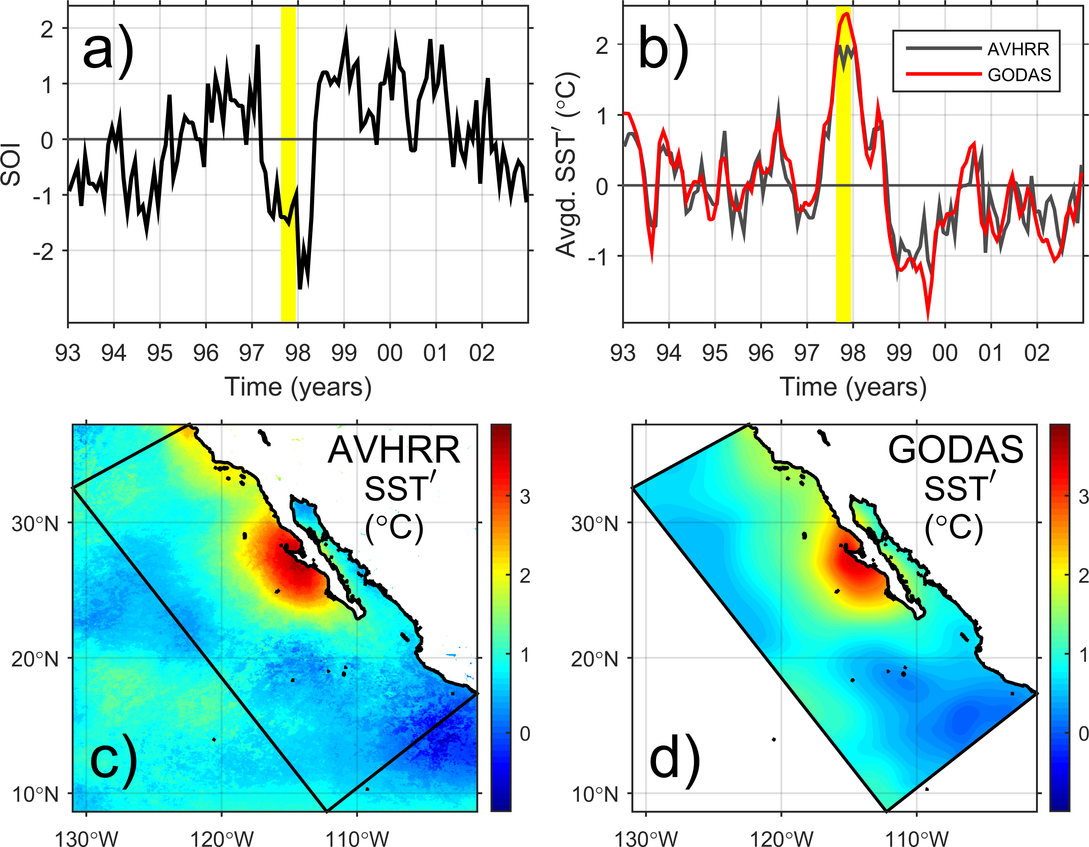
Figure 2 (A) Southern Oscillation Index (SOI), and (B) temporal evolution of monthly-mean, spatially-averaged (within the rectangle shown in panels (C) and (D), which coincides with the model domain) SST anomaly (SST') from AVHRR satellite observations (gray line) and GODAS product (red line), for the 1993-2002 period. Yellow band indicates the September-November 1997 trimester, coincident with the maximum ENSO-induced warming, and period used to calculate the mean SST-anomaly maps shown for the AVHRR (C) and GODAS (D).

The strongest SST anomaly (SST') occurred in September-November 1997 (Figures 2B–D). This El Niño event induced an intense SST positive anomaly off BC peninsula, with a ~2°C peak in the spatially-averaged SST (Figure 2B) and a >3°C mean warm pool (Figure 2C). The GODAS reanalysis product used in the experiments described in Section 2.1 agrees with the satellite SST anomaly (Figure 2D).

The warm pool was linked to a near-surface atmospheric warming, consequence of an anomalous pattern in the synoptic atmospheric surface circulation. By July 1997, a weak and small surface-air warming tendency associated with horizontal heat flux divergence is observable off the southern half of BC Peninsula (23-25°N, 110-113°W, Figure 3A). This tendency is associated with a weakening of the monsoonal winds around the mouth of the Gulf of California and in its interior, and constrained in that zone by an anomalously southwestward wind impulsed by a relatively high pressure forming west of SCB (Figure 3A). This pattern prevails and intensifies by August (1997), when the surface-air warming is relatively stronger and more extensive, and it is constrained by the anomalous flow driven by the high pressure-anomaly which is now stronger and larger (Figure 3B). By September (1997), a large and intense low pressure anomaly dominates the atmospheric circulation west of Mexican waters. It induces a poleward along-shore enhanced flow that induces a surface-air cooling from the Mexican southern coast to the tip of BC Peninsula, and a surface-air warming off the middle portion of BC Peninsula (Figure 3C), resulting in a more intense SST anomaly in this region (Figure 2A). By October (1997), the combination of an elongated trough (linked to the low pressure anomaly which has moved to the southwest) and a small zone of relatively high pressure, features respectively located southwest and south of BC Peninsula, drive a northward flow that intensifies the surface-air warming off BC Peninsula (Figure 3D). This flow turns westward roughly following the isobars between the trough and a high pressure zone located off central California; this circulation also induces a surface-air warming south of Point Conception (Figure 3D). In November (1997), the pattern affecting the southern half of BC Peninsula is weaker, the surface-air warming remains but it is weaker; an enhanced eastward flow dominates the circulation north of 25°N, causing a surface-air cooling along its path onto SCB and the northern portion of BC Peninsula (Figure 3E). By December (1997), the winds around BC Peninsula are weaker, a surface-air cooling is now observed off BC Peninsula, and an intense air-surface warming occurs west of SCB (Figure 3F). By January 1998, the enhanced flow west of SCB reappears but its direction and surface-air cooling are mostly onto regions north of Point Conception. However, part of this flow is directed onto SCB and the northern half of BC Peninsula, forming an along-shore anticyclonic gyre which induces a relatively weak surface-air warming off the southern portion of BC Peninsula (Figure 3G). By February (1998), the enhanced flow has moved southward and it is located west of BC Peninsula, flowing onto the northern half of the Peninsula and driving an along-shore equatorward flow off the southern half, which induces a surface-air cooling off the southern half of the Peninsula and the waters south of it (Figure 3H); the SST anomaly is weakening (Figure 2A). By March (1998), the circulation anomalies are weaker (Figure 3I) and the SST anomaly off BC Peninsula nearly disappeared (Figure 2A).

FIGURE 3

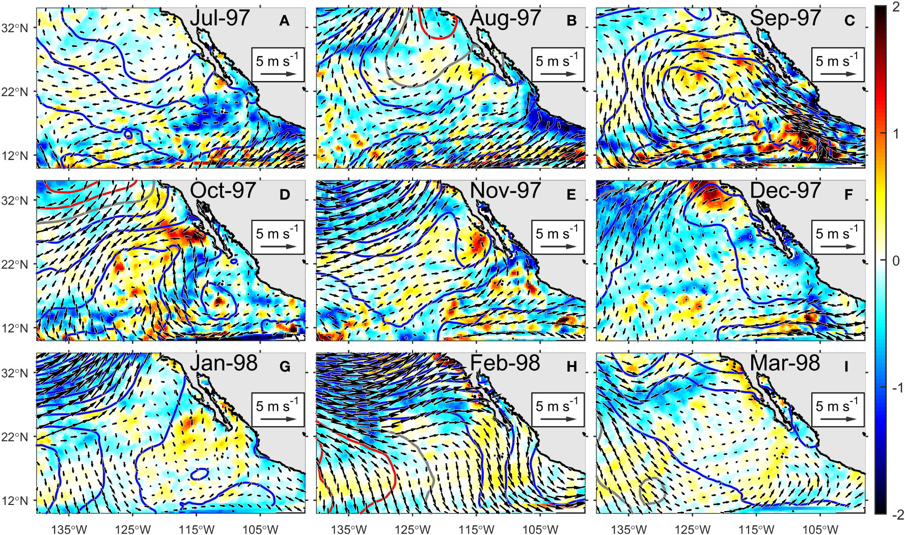
Figure 3 Time sequence of monthly-mean surface atmospheric anomalies from NARR before (A, B, July-August 1997), during (C-E, September-November 1997) and after (F-I, December 1997 – March 1998) the highest SST anomaly associated with the El Niño 1997-98 event. Color corresponds to the temperature-balance quantity $-\nabla •({\text{U}}_{\text{h}}{T}_a)$ in 10^-5°C s^-1 (where ${\text{U}}_{\text{h}}$ is horizontal wind velocity at surface and $T_a$ is air temperature); positive values represent a warming tendency. Contour lines correspond to sea-level pressure (in intervals of 0.5 hPa; blue and red lines are for negative and positive values, respectively, gray line for zero); vectors correspond to surface wind.

3.2 Downscaled reanalysis

We evaluate the capability of the numerical experiments to reproduce the observed SST anomalies. The experiment with prescribed surface fluxes,”ROMS-A” experiment, was unable to fully reproduce the temporal pattern of the SST anomaly (Figure 4A). ROMS-A experiment reproduces well the SST anomaly in its first months but starts to deviate from the observation that reaches its maximum in August 1997. It cools early and ultimately disappears in February 1998, three months before in the observations (Figure 4A). The spatial pattern of the SST anomaly diagnosed by ROMS-A experiment corresponds mostly to broad positive values but does not show the characteristic warm pool off BC Peninsula during September-November 1997, when SST' was the largest (Figure 4C). On the contrary, ROMS-B experiment successfully reproduced both the temporal and spatial patterns of the SST anomaly seen in the observation (Figure 4D).

FIGURE 4

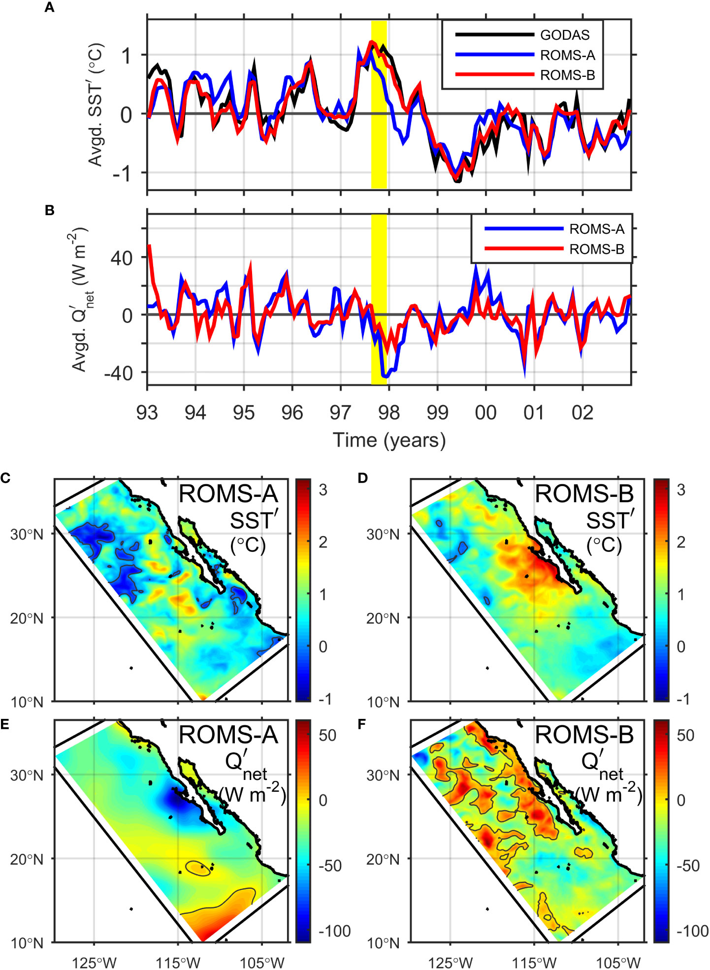
Figure 4 Temporal evolution of monthly-mean, spatially-averaged (within the whole model domain, except the nudging/sponge layer) anomalies of (A) SST and (B) net heat flux from the ROMS-A (blue line) and ROMS-B (red line) reanalysis-downscaling experiments (see Section 2.1), for the 1993-2002 period. Panel (A) also shows the SST anomaly from the GODAS (black line). Vertical yellow bands indicate the September-November 1997 trimester, period for which the mean SST-anomaly (C, D) and mean net heat-flux anomaly (E, F) were calculated for ROMS-A (C, E) and ROMS-B (D, F) experiments. Positive values in net heat-flux anomaly corresponds to an enhanced flux into the ocean.

ROMS-B experiment is generally better reproducing the SST anomaly than ROMS-A, as shown in the Taylor diagram (Taylor, 2001, see Figure 5). In the four evaluated regions, model-data correlations are higher in ROMS-B. As expected, the largest differences are found off BC Peninsula, where the correlation increases from 0.63 in ROMS-A to 0.91 in ROMS-B. Similarly, the correlation increases significantly in the rest of the regions: 0.83 to 0.91 in Southern California Bight (SCB), 0.71 to 0.88 in Tropical Eastern Pacific (TEP), and 0.77 to 0.90 in the Gulf of California (GoC). Standard deviation ratios are also improved in ROMS-B, with values closer to 1 expect for the TEP (where they are ~ 0.5 but still better than those in ROMS-A), and the RMSD values are also lower in this experiment.

FIGURE 5

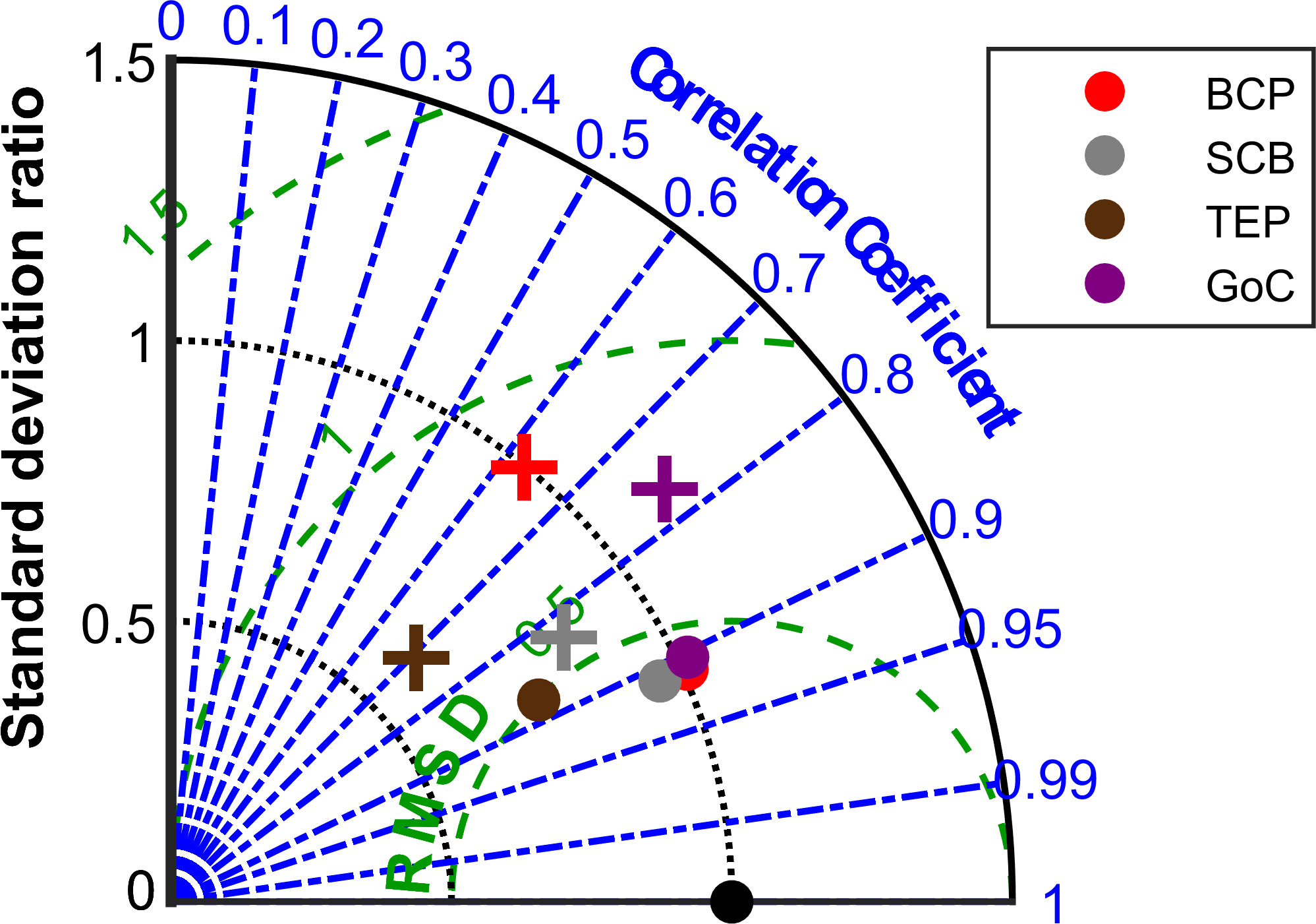
Figure 5 Taylor diagram for monthly SST-anomaly values located within the regions shown in Figure 1 during September-November 1997 (spatio-temporal arrays expressed as series of consecutive data), from ROMS-A (plus signs) and ROMS-B (dots) experiments. Radial distance represents the ratio of simulated to observe standard deviations and azimuthal angle represents model-observation correlation. All the correlation calculations satisfy $p<0.05$. Observations coincide with the location defined by standard deviation ratio and correlation equal to one (black dots). Interior dashed contours show the root-mean-square deviation (RMSD). Marker colors indicate the data’s regions: BC Peninsula (BCP), Southern California Bight (SCB), Tropical Eastern Pacific (TEP), and Gulf of California (GoC).

These results emphasize the importance of the surface fluxes in reproducing the SST anomaly, as it is the only difference between the two experiments. The maximum differences in SST anomalies between the experiments are associated with large differences in heat-flux anomalies. These differences are maximum in November-December 1997, when ROMS-A simulation has a strong negative anomaly ~ -40 W m^-2 that is 2 times greater than the negative anomaly ~ -20 W m^-2 from ROMS-B simulation (Figure 4B). The mean net-heat flux anomaly (in September-November 1997) off BC Peninsula in the two experiments are opposite between each other, ROMS-A [prescribed fluxes] shows an intense upward flux (ocean’s cooling) ~ -100 W m^-2, whereas ROMS-B [internally-calculated fluxes] shows a downward flux (ocean’s heating) ~ 50 W m^-2 (Figures 4E, F).

3.3 Controls on ENSO-driven SST anomalies

3.3.1 EOF analyses

As mentioned in the previous section, the SST warm anomaly localized off BC Peninsula, reproduced by ROMS-B experiment, is apparently linked to an anomalous surface-air warming driven by the synoptic circulation. In addition, the downward longwave-radiation anomaly must contribute to the modulation of the SST anomaly, although to a lesser extent. It shows high values (enhanced radiation flux into the ocean) in the last months of 1997 (not shown), when the SST anomaly was most pronounced, and reverse (radiation flux out of the ocean) in March-April 1998, when the SST anomaly decreases. Along-shore wind-stress anomaly are essentially the same in both experiments (i.e. minor changes in the internally-calculated drag coefficient) and it is mostly poleward through the year 1997 (Figure 3), which implies a weakening of upwelling favorable winds.

As described in Section 2.1, an EOF analysis was carried out in order to elucidate the most important atmospheric variables in the surface fluxes calculations. The 1^st variation mode of the SST anomalies, corresponds to a warming in the whole model domain with a warmer band perpendicular to the southern part of BC Peninsula, extending from the coast through the model’s western boundary, and where the coastal area corresponds to the ENSO-induced warm pool (Figure 6A). This 1^st mode explains 54% of the variance contained in the SST anomalies.

FIGURE 6

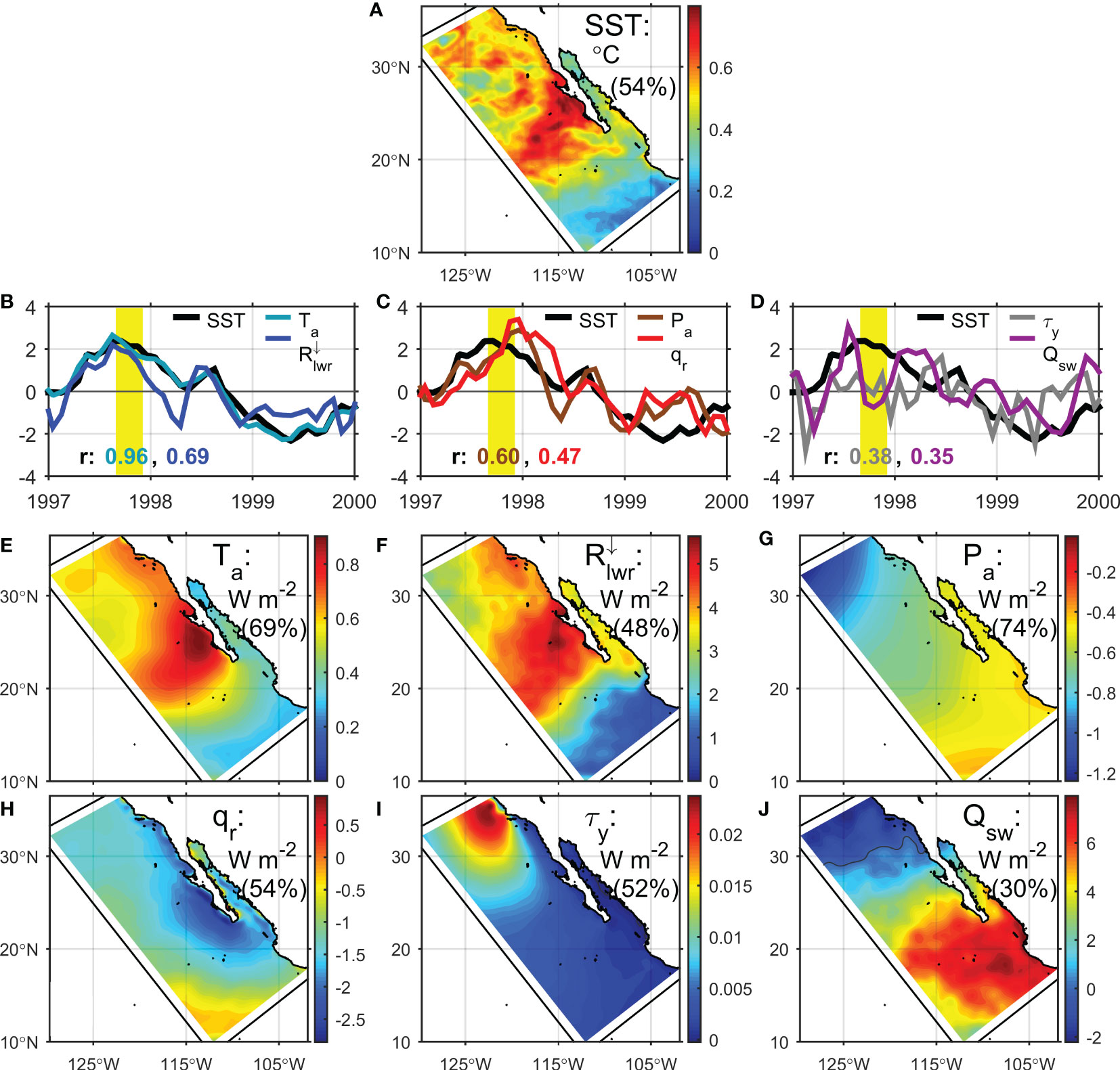
Figure 6 Comparison between the first EOF mode of the SST anomaly (see Section 2.1) from ROMS-B experiment (A) and those of the atmospheric fields provided to the model: air temperature ($T_a$; in °C), downwelling longwave radiation ($R_{lwr}^{\downarrow }$; in W m^-2), air pressure ($P_a$; in hPa), relative humidity ($q_r$; in percentage), along-shore wind stress (${\tau }_y$; in N m^-2), and net shortwave radiation ($Q_{sw}$; in W m^-2). Only those variables with a significant correlation ($p<0.05$) are shown. Panels (B-D) shows comparisons of the principal components (time series of amplitudes), panels (E-J) shows the EOF spatial structures. Percentage of explained variance for each variable is indicated.

The principal component (i.e. the eigenvalue or amplitude time series; PC) of the SST-anomaly 1^st mode described above was compared to those of the meteorological variables used to force the model, in order to explore their importance. Table 1 and Figures 6B–J show these correlation results. Air temperature 1^st PC, which explains 69% of variance of this variable’s anomaly, has the highest correlation ($r=0.96$) with that of the SST anomaly, and the highest values of its 1^st EOF coincide with those of the SST 1^st EOF (Figures 6B, E). The second most correlated 1^st PC ($r=0.69$) is that of the downward longwave radiation anomaly explaining 48% of its variance, shows a spatial pattern consistent with those of air temperature and SST (Figures 6B, F). Atmospheric pressure 1^st PC (74% of its anomaly variance) has also a relatively high correlation with that of SST ($r=0.60$). In this case the main features of its EOF was a low-pressure signal located northwest of BC Peninsula, consistent with that shown in Figure 3E. Results from the other three variables in Figure 6 show lower but still significant correlations ($r<0.50$) with the SST 1^st mode (Figures 6C, D). Relative humidity shows a negative signal around BC Peninsula (Figure 6H), consequence of the less-saturated, warm-air signal mentioned above, and of the positive signal of downward long-wave radiation affecting the Peninsula (Figure 6J). The along-shore wind-stress signal occurs as an intensification west of Point Conception (Figure 6I), associated with the low-pressure signal in that region.

TABLE 1

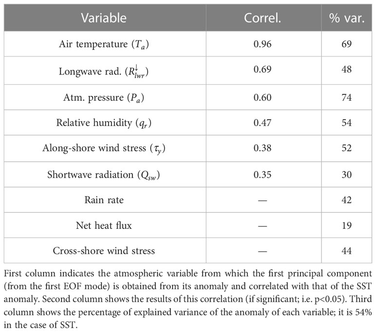
Table 1 Results from the EOF analysis described in Section 2.1.

3.3.2 Sensitivity to individual forcing fields

The EOF analysis described previously provides an insight about which atmospheric variables are important to reproduce the ENSO-induced warm pool, but the results relies on linear statistics. Therefore, herein we carried out sensitivity experiments in order to further evaluate the contribution of each atmospheric variable anomaly to the surface fluxes and hence to the ENSO-induced warming off BC Peninsula. As described in Section 2.1.1, shorter simulations (March 1997 - September 1998) were done in which the interannual variability of each atmospheric variable was removed by substituting its original values by its mean seasonal cycle. Correlations, RMS error, and MD between monthly SST anomaly from each sensitivity simulation and the original experiment were calculated for a coastal box located off BC Peninsula (purple box in Figure 1) that is centered on the region of maximum SST values. Lower correlations and larger RMS errors imply a higher importance of the analyzed forcing variable. Based on these criteria, air temperature and wind stress are the most important variables (Table 2). Similarly, for the 3-month period centered in the SST anomaly peak (September-November 1997) air temperature and wind stress are still the most important variables but their order of importance changes (Table 3).

TABLE 2

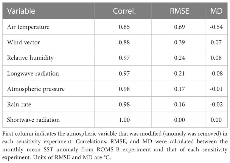
Table 2 Statistical results from the sensitivity reanalysis-downscaling experiments (see Section 2.1.1) for the period from March 1997 to September 1998.

TABLE 3

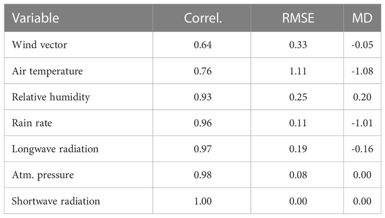
Table 3 Same as Table 2 but for the shorter period from September to November 1997.

In spite of the results shown in Tables 2, 3, modifying only the wind field has a moderate effect on the simulation (Figures 7A, B), just increasing the magnitude of the SST peak (Figure 7A). Air temperature, on the other hand, shows a major effect on the warm pool (Figure 7C). Interestingly, the net heat flux is similar in both experiments, showing a positive anomaly off BC Peninsula (Figures 7D, E); this situation will be discussed in Section 4.

FIGURE 7

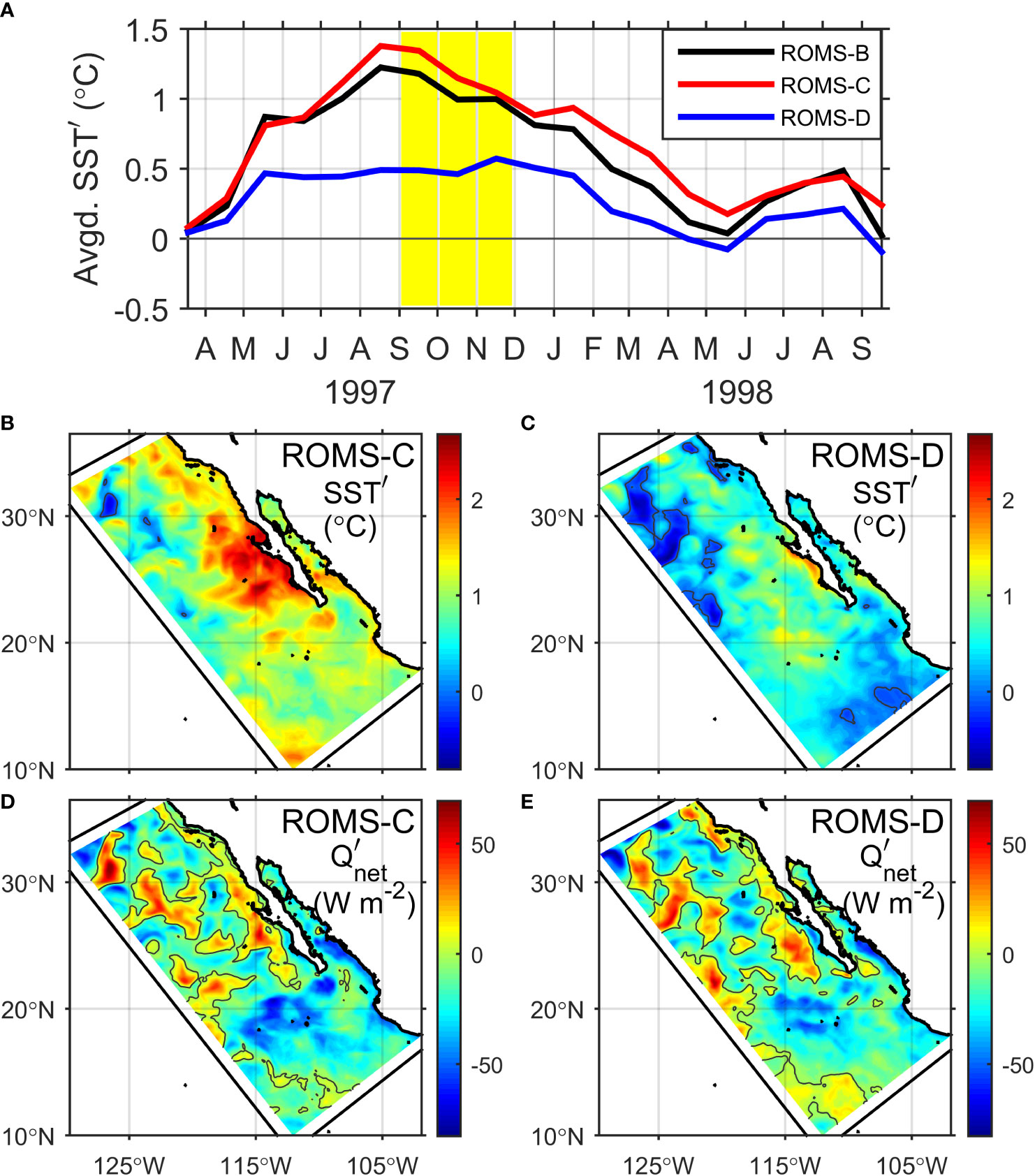
Figure 7 (A) Temporal evolution (from March 1997 to September 1998) of monthly-mean, spatially-averaged (within the whole model domain, except the sponge layer) SST anomaly from ROMS-B experiment (black line), and from two sensitivity reanalysis-downscaling experiments (see Section 2.1.1): removing the interannual variability of the wind (ROMS-C; red line) and the air temperature (ROMS-D; blue line). Yellow band indicates the September-November 1997 trimester, period for which the mean SST-anomaly (B, C) and mean net heat-flux anomaly (D, E) were calculated for ROMS-C (B, D) and ROMS-D (C, E) experiments.

3.3.3 Surface heat-flux components

Further detail about the surface heat flux involved in the formation of the warm pool off BC is herein presented by the quantification of each of the air-sea heat-flux components in Eq. (2). Input/output variables from the model simulations were taken to quantify these heat-flux components, except for the net long-wave radiation flux which was not saved in the model’s output files, hence it is estimated using Eq. (5) [with $T_s=\text{SST}$] for the case of ROMS-B experiment. Table 4 shows the mean flux anomalies within the coastal box off BC during the SST-anomaly peak. Notice that the values of $Q_{net}$ do not exactly match the sum of four heat-flux components, these discrepancies can be associated with errors in averaging, interpolation (Reanalysis-to-model interpolation of input variables), and/or calculation (monthly-mean instead of instantaneous SST in $Q_{lwr}$).

TABLE 4

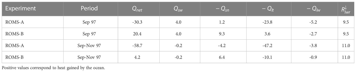
Table 4 Mean anomalies of the surface heat-flux budget (W m^-2) given by Eq. (2), spatially-averaged within the coastal box off BC Peninsula shown in Figure 1, from ROMS-A and ROMS-B experiments, for September 1997 and September-November 1997.

In September 1997, when the maximum SST anomaly occurred, ROMS-A experiment presents a net heat loss ($Q_{net}=-30.3$ W m^-2) in contrast with ROMS-B which presents a net heat gain ($Q_{net}=20.4$ W m^-2) [Table 4]. In both experiments the short-wave radiation flux is the same, in this case with a positive anomaly ($Q_{sw}=4.0$ W m^-2) which corresponds to an anomalous heat input by the solar irradiance (Table 4). On top of this heat gain, there is a net gain by sensible heat flux ($Q_{sn}$) in both cases, but this is ~10 weaker in ROMS-A ($1.2$ W m^-2) with respect to ROMS-B ($9.3$ W m^-2). There is also a net heat gained by latent heat flux ($Q_{lt}$) in ROMS-B (3.6 W m^-2) but not in ROMS-A, where the latent flux is negative and remarkably strong (-23.8 W m^-2). In both experiments there is a heat loss by long-wave radiation flux ($Q_{lw}$), which is 2 times stronger in ROMS-A (-5.2 W m^-2 vs. -2.7 W m^-2 in ROMS-B); the downward long-wave radiation flux is the same in both experiments ($R_{lwr}^{\downarrow }=9.5$ W m^-2) [Table 4].

In the whole September-November 1997 trimester, the net heat loss in ROMS-A is stronger (-58.7 W m^-2) compared to the one mentioned above for September, and the net heat gain (4.2 W m^-2) in ROMS-B is weaker (Table 4). The remarkably strong heat loss in ROMS-A is responsible for the early decrease of the SST anomaly in that experiment. The anomaly of short-wave radiation flux is nearly null ($Q_{sw}=-0.2$ W m^-2) and has a negligible contribution to the heat budget. In ROMS-A the ocean surface losses heat by all the four heat-flux components, especially by latent flux which contributes to 85% of the lost heat. In ROMS-B there is a positive sensible-heat flux anomaly ($Q_{sn}=6.4$ W m^-2) which compensates and even exceeds the negative net heat-flux anomaly ($Q_{net}$), but it is not strong enough to compensate the heat loss driven mostly by latent-heat flux ($Q_{lt}=-10.1$W m^-2). We note that although the budget residual is large, the dominance of $Q_{lt}$ is illustrated in the Discussion.

3.4 2015-16 El Niño event

As shown in the previous sections, during intense warm conditions like those in the 1997-98 El Niño event, a model configuration with prescribed surface fluxes (ROMS-A experiment) can present important limitations with respect to one where these fluxes are internally calculated (ROMS-B experiment), and that distinctive atmospheric patterns are associated with this warming. To establish whether these features are exclusive to the 1997-98 event or they occur in other ENSO-induced warm events, herein we diagnose the surface anomalies associated with the 2015-16 El Niño event, responsible for an intense warming off BC Peninsula (Dorantes-Gilardi and Rivas, 2019), from the extended ROMS-A and ROMS-B experiments described in Section 2.1.2. There are remarkable similarities between both El Niño events. In this more recent event (2015-16) the maximum SST anomaly off BC occurred in October 2015 (Dorantes-Gilardi and Rivas, 2019). This peak is reproduced by the ROMS-B experiment but not by the ROMS-A, since the latter experiment underestimates the SST anomaly from October 2015 to April 2016, even presenting negative anomalies from November 2015 to January 2016 (Figure 8A). This underestimation is associated with an excessively large heat-loss in ROMS-A with respect to that in ROMS-B (Figure 8B). The SST anomaly is more intense off the southern half of BC peninsula (Figures 8C, D) but it does not exist in the ROMS-A experiment which even shows negative values off the whole peninsula (Figure 8E). As in the 1997-98 El Niño event, distinctive features of the atmospheric circulation play an important role in the formation of the warm pool off BC in the 2015-16 event. In particular for the mean atmospheric anomalies in the last three months of 2015, a low pressure located south of BC peninsula, which drives winds coming from the south and the Gulf of California, together with a high pressure located northwest of the Peninsula driving wind from the SCB, cause a convergence of heat off the middle portion of the Peninsula (Figure 8F), which must supply heat onto the ocean surface to generate the characteristic warm pool. Then, all these anomalous patterns seem to be recurrent in intense ENSO-induced warm anomalies off BC, which strengthen the results presented in the previous sections.

FIGURE 8

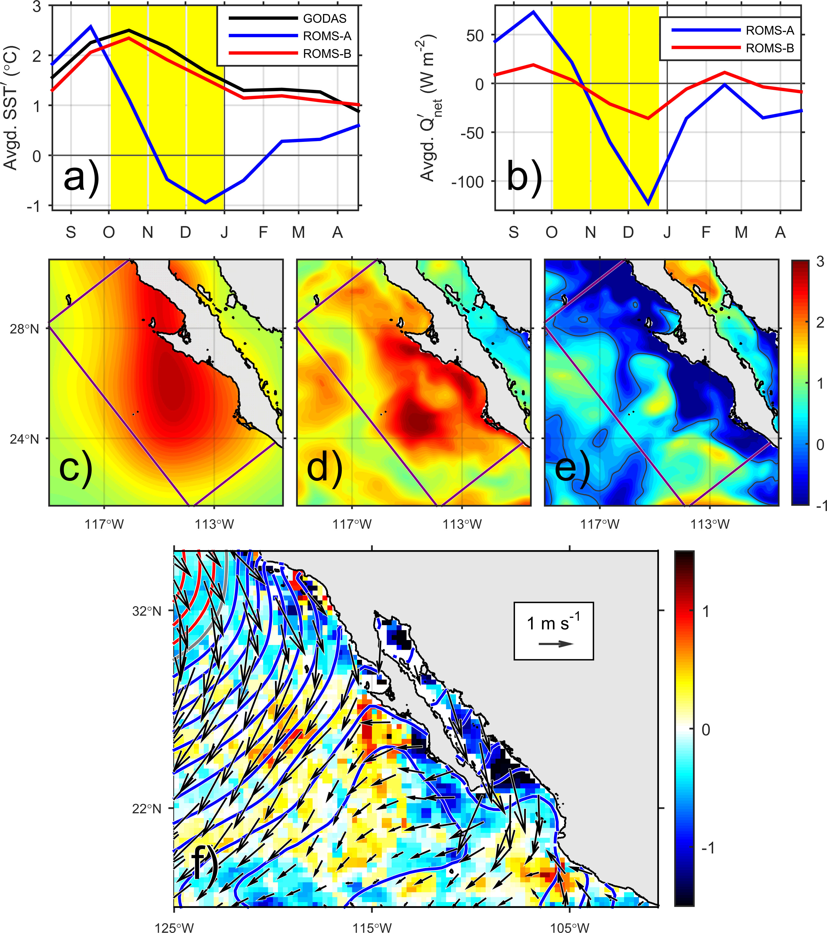
Figure 8 Upper row (A, B): Same as Figure 4A, B, but spatially-averaged within the coastal box off BC Peninsula (“BCP” in Figure 1) and for the period from August 2015 to May 2016. Vertical yellow bands indicate the October-December 2015 trimester, period for which the mean SST anomaly (°C) was calculated from the GODAS product (C), and ROMS-B (D) and ROMS-A (E) experiments. Lower row (F): Similar to Figure 3, but for the October-December 2015 mean, and with pressure contour lines in intervals of 0.2 hPa. The anomalies are defined with respect the 1993-2002 climatology.

4 Discussion

The localized and intense SST anomaly off BC Peninsula is mostly a response to an atmospheric pattern associated with the El Niño. During the months when the maximum SST anomaly is observed (September-November 1997) the eastern Pacific off Mexico was dominated by an sea-level pressure trough extending with a cyclonic circulation which favored an anomalous flow from near-equatorial regions. This anomaly weakened the coastal upwelling and also produced an advective warming of the surface air. As shown in our experiments, this near-surface atmospheric warming is of paramount importance in the heat fluxes off BC Peninsula. Also, anomalies in the local coastal upwelling (changes in sea surface temperature) would be associated with anomalies in the ocean-to-land air-moisture transports (Reimer et al., 2015), which must influence the local humidity (and low-level cloudiness) and hence the downward long-wave radiation, a secondary forcing field in our simulations. However, notice that even if the downward long-wave radiation ($R_{lwr}^{\downarrow }$) shows the second highest correlation with the SST anomaly in our EOF analysis (Section 3.3.1), it is its difference with the outgoing (upward) long-wave radiation which contributes to the net heat flux. $R_{lwr}^{\downarrow }$ is correlated with the air temperature ($r=0.71$), which is in turn highly correlated with the SST ($r=0.94$); SST is also correlated with the outgoing long-wave radiation ($r=0.66$), which results in that the remainder between this outgoing radiation and $R_{lwr}^{\downarrow }$ is not significantly correlated with the SST anomaly. On the other hand, the synoptic-scale near-surface circulation (enhanced westerly zonal winds in the eastern North Pacific), typical of strong El Niño conditions (Cavazos and Rivas, 2004), also plays an important role in the regional ENSO-induced warming since it modulates the advection of heat and moist from sub-tropical regions. From all the results, we can emphasize the need of a proper representation of the near-surface atmospheric patterns associated with the El Niño phenomenon.

Although our analysis is focused on the El Niño event that occurred in 1997-98, the results are applicable to other intense El Niño episodes, as shown by the additional simulation for the 2015-16 period (Section 3.4). This event shows a warm pool off BC, net heat-flux anomalies, and anomalous atmospheric patterns comparable to those in the 1997-98 event (Figure 8). Also in this 2015-16 event and like in the 1997-98 event, the numerical simulation based on the ROMS-A configuration presented limitations to fully reproduce the timing of the warm pool, showing an early decrease of the SST as it reached its maximum in the observational data (Figure 8A). A similar failure occurred in a previous numerical-modeling study for northwestern BC during this same 2015-2016 event (Dorantes-Gilardi and Rivas, 2019), which had a model configuration essentially similar to the ROMS-A experiment, and this failure limited the analysis of the effects of thermal anomalies on biogeochemical variables in that region. As in our analysis, an excessive heat loss (Figure 8B) may have been responsible for that failure, which could have been solved using internally-calculated surface fluxes (i.e., ROMS-B configuration) to make the modeled warm pool more realistic (Figures 8C, D).

The evaluation of the surface heat-flux budget (Table 4) shows that the latent heat flux has a major role in the anomalous net air-sea heat exchange compared to the other heat-flux components. A simplified but illustrative calculation of the heat-flux components in Eq. (2) was carried out in order to understand the response of its components to a surface warming. To do this, Eqs. (3)-(5) were evaluated for a constant, mean air-sea state within the coastal box off BC Peninsula (Figure 1) but with $\text{SST}=T_s+\text{Δ}T$, with $-3^{\circ }\text{C}\le \text{Δ}T\le 3^{\circ }\text{C}$. The values for the air-sea variables were taken from the input/output model variables for November 2001, when the monthly-mean SST anomaly was practically null and it could be a climatological state (at least in terms of SST) in which the SST anomaly would be set to $\text{Δ}T$. The results of these calculations are shown in Figure 9A. The latent-heat flux ($Q_{lt}$) has a more abrupt response to the thermal variation compared to the sensible-heat and long-wave radiation fluxes, it can be more than double when $\left|\text{Δ}T\right|=3^{\circ }\text{C}$ (Figure 9A). This explains why the latent flux responds faster to the thermal variations and is more important during the formation of the warm pool, which implies that most of the heat lost to the atmosphere is driven by a vigorous evaporation triggered by surface warming.

FIGURE 9

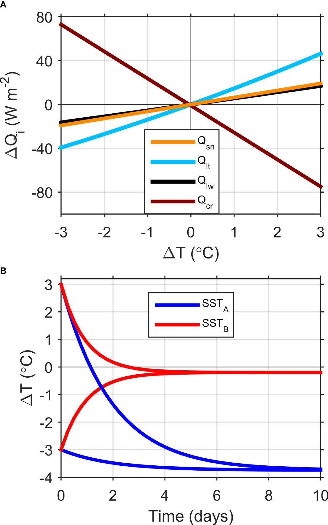
Figure 9 (A) Evaluation of the heat-flux components ($Q_i$; where $i=sn$ for sensible, $i=lt$ for latent, $i=lw$ for long-wave radiation, and $i=cr$ for bias-correction) in Eqs. (3)-(5) described in Section 2.3.1 for $\text{SST}=T_s+\text{Δ}T$ (i.e., adding a temperature variation to a “mean” state $T_s$), and the correction term defined by Eq. (1). The heat-flux results are expressed as variations with respect to the mean state, and as functions of the temperature change $\text{Δ}T$. (B) Solutions of the simplified temperature balance defined by Eq. (8), using the ROMS-A and ROMS-B model configurations, with two different initial values ($\text{Δ}T=\pm 3^{\circ }\text{C}$) in each case. In both panels (A, B), The temperature results are expressed as deviations with respect the mean state, and as functions of the integration time. The following values were used for the air-sea variables: $T_s={20.8}^{\circ }\text{C}$, $T_a={17.0}^{\circ }\text{C}$, $q_a=0.011$, $P_a=1018.4$ hPa, ${\rho }_a=1.22$ kg m^-3, $U=5.2$ m s^-1, $R_{lwr}^{\downarrow }=348.2$ W m^-2. ${\rho }_0=1024.4$ kg m^-3, ${(\text{d}{Q}_{net}/\text{d}{T}_s)}_{ref}=-24.6$ W m^-2°C^-1, and $T_{ref}={20.7}^{\circ }\text{C}$.

Herein we have described the advantages of using internally-calculated surface fluxes in the model configuration, however, another important factor that contributes to obtain better numerical solutions (starting with SST) is the correction term $Q_{cr}$ given by Eq. (1). As the surface heat flux is a strong function of temperature, this correction term is of paramount importance to update the net heat flux $Q_{net}$ according to the instantaneous SST and to prevent the model to drift away from the reference temperature. Figure 9A shows the evaluation of Eq. (1) at $\text{SST}=Ts+\text{Δ}T$, using the same air-sea “mean” state mentioned above. Compared to the heat fluxes, $Q_{cr}$ varies about twice faster with the temperature, which can result in an efficient adjustment of $Q_{net}$. In spite of how efficient this correction can be, its contribution is limited. To show how $Q_{cr}$ works in the two model configurations (ROMS-A and ROMS-B), here we solve the simplified temperature balance given by

$\begin{array}{ll}\frac{\partial \text{SST}}{\partial t}=\frac{1}{{\rho }_0{C}_p}(Q_{net}+Q_{cr}),& (8)\end{array}$

where ${\rho }_0$ and $C_p=4000$ J kg^-1° C^-1 are the density and the specific heat capacity of sea water; these results are shown in Figure 9B. Regardless of whether the initial temperature is higher ($\text{Δ}T=3^{\circ }\text{C}$) or lower ($\text{Δ}T=-3^{\circ }\text{C}$) than its mean value, the instantaneous temperature converges to a nearly constant value after 8 days in the ROMS-A configuration, and only 4 days in the ROMS-B configuration. More importantly, the final value obtained in ROMS-B approaches to the reference temperature at $\text{Δ}T=T_{ref}-T_s=-{0.04}^{\circ }\text{C}$, whereas the final value in ROMS-A presents a bias of ~ -3.7°C with respect to the reference temperature (Figure 9B). This bias results from the balance between the constant $Q_{net}$ value, which makes the solution change indefinitely at a linear rate, and the $Q_{cr}$ term, which approaches to $T_{ref}$. The relation among the heat fluxes and other variables involved in $Q_{net}$ and $Q_{cr}$ determines not just the amplitude of the bias in ROMS-A, but also the rate of change of the solution. Then, these results emphasize the possible limitations of the ROMS-A model configuration to prevent bias in the SST and thus in other physical variables.

As the model runs, the heat-flux components interact between each other to produce a net surface forcing that modifies the SST, and this change in turn modifies the heat-flux components. The combination of these forcings and feedbacks will determine the values of the resulting SST anomalies, which can be different in each experiment and not necessarily intuitive. For example, ROMS-C and ROMS-D experiments, in which the interannual variabilities of wind (ROMS-C) and air temperature (ROMS-D) were respectively removed, show a net heat flux that is similar in both cases even if the SST anomaly is different between each other (Figures 7D, E). Based on estimates with Eqs. (2)-(5) for September-November 1997 (using air-sea variables averaged for this period and within the coastal region off BC Peninsula) both increasing the wind speed and reducing the air temperature (wind was 4% weaker and air temperature was 1°C higher than their climatological mean values in September-November 1997) cause an ocean heat loss [$\text{Δ}{Q}_{net}=-3.3$ W m^-2 (ROMS-C), -5.1 W m^-2 (ROMS-D)] and hence a decrease in SST [$\text{ΔSST}=-{0.2}^{\circ }\text{C}$ (ROMS-C), −0.3°C (ROMS-D)]. Based on the inverse $\text{Δ}{Q}_i$ - $\Delta \text{SST}$ relation (Figure 9A), this negative SST change would cause a positive change in $Q_{net}$ [$\text{Δ}{Q}_{net}=+4.4$ W m^-2 (ROMS-C), +6.6 W m^-2 (ROMS-D)], together with a positive $Q_{net}$ compensation by Eq. (1) [$Q_{cr}=+4.1$ W m^-2 (ROMS-C), +6.5 W m^-2 (ROMS-D)], which in turn would cause a subsequent increase in SST. These rough estimates emphasize the fact that the cooling caused by the original wind and air-temperature anomalies can be compensated and even exceeded by a feedback warming. However, during the model’s run these opposing processes act simultaneously to produce a continuously updated forcing which can result in a different final state. On the other hand, ROMS-C presents the relevant difference that modifying the wind causes changes in the sea surface circulation, which can be especially important in near-coastal areas. The anomalously weak wind would cause a decrease in the coastal upwelling and hence the offshore advection of colder water from subsurface levels. This dynamical factor, driven by the momentum flux applied by the surface wind, has direct effects on the SST and the air-sea exchanges, resulting in marked differences of its effects with respect to other atmospheric variables like the air temperature, as well as the magnitude of the SST anomalies.

The heat-flux calculation implemented in this paper has been previously used by other authors. Deutsch et al. (2021) were able to reproduce the 1997-98 El Niño event in the California Current System in a historical simulation with ROMS, computing also online surface heat fluxes and wind stress with instantaneous modeled fields (Renault et al., 2021). In contrast with our paper, these works lack an accurate analysis of ocean physical variables during the El Niño event and they do not identify that online computation of surface forcing with instantaneous modeled fields is critical for the reproduction of ENSO-driven phenomena in the ocean.

Intense El Niño events like the one analyzed in this paper (1997-98) has effects on other oceanic variables in addition to the SST. These effects can be directly or indirectly associated with the regional warming described in the previous sections. In our nested reanalysis, a positive sea-level anomaly ~5 cm - located along the coast from south of Cabo Corrientes to north of Point Conception, with greater values (8-10 cm) seaward from the shelf (Figure 10A) - occurred during the maximum SST event. This anomaly is consistent with coastal observations off central California which show positive sea-level anomalies associated with El Niño events, attributed to the passage of remotely generated and coastal trapped waves that were generated along the equator and propagated to the north along the west coast of North America (Ryan and Noble, 2002).

FIGURE 10

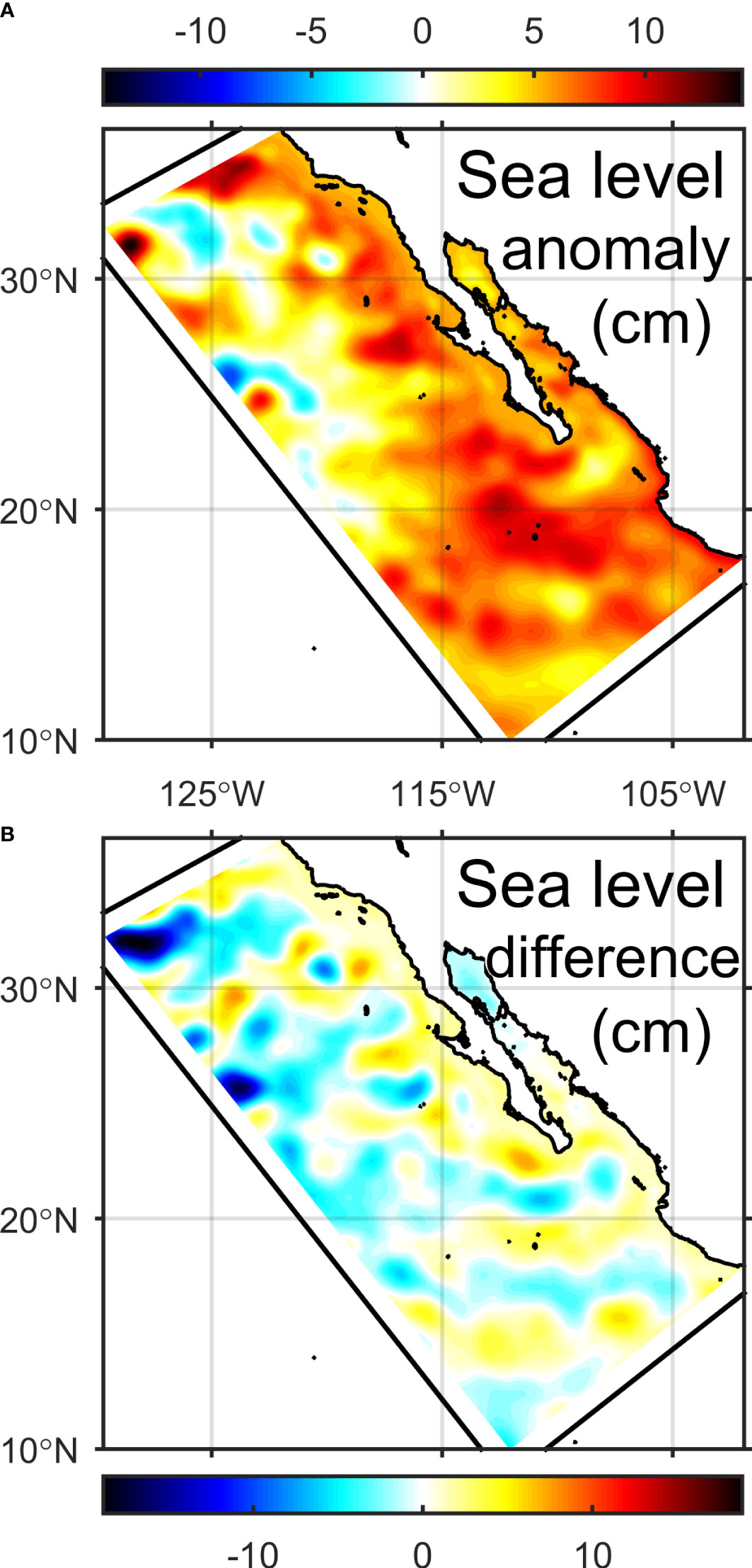
Figure 10 September-November 1997 means of (A) sea level anomaly from ROMS-B, and (B) sea level (climatology plus anomaly) from ROMS-B minus that from ROMS-A.

The physical anomalies described above can have important effects on the biogeochemical variables. As concluded from previous numerical-modeling results, an ENSO-induced regional warming strengthens the stratification that limits the vertical and onshore transport of nitrate onto the upper levels, and results in a subsurface reduction of nutrients (Dorantes-Gilardi and Rivas, 2019). This conclusion is consistent with hydrographic-observational results in the southern California Current System: a deepening of the nutricline off BC Peninsula has been reported during El Niño episodes, especially near the coast (Gaxiola Castro et al., 2010) and, specifically for the 1997-98 period, a deepening of the nutricline and nutrient depletion in the upper levels (from 80-m depth to the surface), associated with positive temperature anomalies at subsurface, was reported for central California from August 1997 through August 1998 (Castro et al., 2002). The chlorophyll field is consequently affected, as corroborated by in-situ observations of depth-integrated (0-100 m) chlorophyll-a anomalies off BC Peninsula, which showed a negative anomaly during the peak of the 1997-98 El Niño (McClatchie et al., 2016). It has been argued in previous literature (Dorantes-Gilardi and Rivas, 2019) that a regional warming deepens the thermocline and hence moving the subsurface chlorophyll maximum downwards, causing a reduction in the phytoplankton biomass. The oxygen field can be also affected by the regional warming, since its variability in the ocean upper levels is driven by changes in temperature and, in near-coastal areas, by changes in coastal upwelling (e.g. Turi et al., 2018). Thus, an anomalous downwelling (weakening of upwelling-favorable conditions) caused by the poleward coastal-wind anomaly like that in September-November 1997 (Figures 3C–E) must induce positive oxygen anomalies along the coast, given the reduced presence of oxygen-poor water from deeper levels. An opposite effect would be expected in offshore regions, where negative oxygen anomalies can occur, associated with a decreased oxygen solubility caused by the increased temperature. These results and notions are somewhat consistent with recent numerical results (Deutsch et al., 2021), which show that the amplitude of interannual variability in nitrate at the base of the photic zone and of oxygen in the thermocline are also both strongly correlated to undulations of the pycnocline, and the largest such anomalies in our simulation period were associated with the 1997-98 ENSO event.

Failing to reproduce the regional warming adequately implies an underestimation of the El Niño teleconnection on oceanic variables. For example, a comparison between two reanalysis-downscaling experiments (one using directly atmospheric forcing and once recomputing them with bulk formulae) suggests an underestimation of ~3 cm in the coastal sea level by the former experiment (Figure 10B), about 50% the coastal anomaly (Figure 10A). This underestimation will introduce large model biases in the biogeochemical fields.

5 Conclusions

Downscaling of global reanalysis products for a region of interest is a tractable alternative for reproducing many of the dynamical features typical of that region that are not resolved in coarse climate prediction and reanalysis systems. These local dynamics are associated with morphologic and physical characteristics of paramount importance. Here we demonstrate that one-way offline nesting of a three-dimensional regional model with global reanalysis products improves the representation of the local anomaly for the warming off Baja California Peninsula associated with the 1997-98 El Niño event (results also corroborated for the 2015-16 El Niño event). This episode is one of the most intense El Niño episodes in the last decades. Given the important environmental effects of the ENSO on the Pacific Ocean and other regions, improving its representation in numerical simulations and its implication onto the coastal regions will enhance the usefulness of seasonal predictions (Kirtman et al., 2014). We have shown that an accurate representation of the surface fluxes is of paramount importance to reproduce the ENSO-induced SST anomalies. Prescribed heat fluxes can be inadequate for the regional model since they cannot “accommodate naturally” to the atmospheric conditions provided to the model. Internally-calculated surface fluxes provide the possibility to the model to “adjust” to the atmospheric conditions, as the instantaneous SST is taken for the net heat flux calculation. Nonetheless, it is necessary that the atmospheric fields used to force the model are able to represent the ENSO-driven atmospheric circulation over the Northeastern Pacific, because it is responsible for the advection of warm and humid air onto the near-surface atmosphere off Baja California Peninsula, coming from near-equatorial regions and also from relatively warmer regions from the central Pacific. The atmospheric pattern, specifically the wind anomaly observed as an along-shore wind stream, would also cause weakened upwelling conditions along the Baja California coast during the period of the maximum SST anomaly, contributing to the coastal warming, and enhanced upwelling conditions by the end of the SST anomaly, counteracting the coastal warming and probably helping to cause the disappearance of the regional SST anomaly. Thus, the numerical exercises described in this paper will provide valuable insights to improve the reproducibility of ENSO thermal anomalies and similar signals and open the possibility to asses downscaling of seasonal prediction there.

Data availability statement

The raw data supporting the conclusions of this article will be made available by the authors, without undue reservation.

Author contributions

DR implemented and ran the numerical model, processed and analyzed the data, and wrote and edited the manuscript. FC was host and provided funding, helped with the model implementation, and revised the manuscript. NK was host and provided funding, revised the manuscript. All authors contributed to the article and approved the submitted version.

Acknowledgments

We thank the reviewers for their critical comments and suggestions to an earlier version of this manuscript, especially “Reviewer 1”, whose thorough review really enriched this paper. This research was carried out during a sabbatical visit of DR to the NERSC and GFI-UiB in Bergen, Norway, which was funded by project CONACYT-ERC 297701 and from the Strategic Programme for International Research Collaboration from the University of Bergen 2019. During this visit, DR received funding from the Bjerknes fellowship and SPIRE 2019 programmes. DR was also supported by CICESE through the internal project 625118. FC and NK acknowledge the NFR-Climate Futures (309562) and the Trond Mohn Foundation, under project number BFS2018TMT01. This work has also received a grant for computer time from the Norwegian Program for supercomputing (NOTUR2, project number nn9039k) and a storage grant (NORSTORE, NS9039k). The work was also supported from the European Union’s Horizon 2020 research and innovation programme under grant agreement No 817578 (TRIATLAS). The GODAS and NARR products were provided by the National Oceanic and Atmospheric Administration (NOAA) - Earth System Research Laboratory (ESRL) Physical Science Division (PSD) through its website: http://www.esrl.noaa.gov/psd/data/gridded/.

Conflict of interest

The authors declare that the research was conducted in the absence of any commercial or financial relationships that could be construed as a potential conflict of interest.

Publisher’s note

All claims expressed in this article are solely those of the authors and do not necessarily represent those of their affiliated organizations, or those of the publisher, the editors and the reviewers. Any product that may be evaluated in this article, or claim that may be made by its manufacturer, is not guaranteed or endorsed by the publisher.

References

Adem J. (1967). Parametrization of atmospheric humidity using cloudiness and temperature. Mon. Wea. Rev. 95, 83–88. doi: 10.1175/1520-0493(1967)095<0083:POAHUC>2.3.CO;2

CrossRef Full Text | Google Scholar

Amante C., Eakins B. W. (2009). ETOPO1 1 arc-minute global relief model: procedures, data sources and analysis. NOAA Tech. Memorandum NESDIS NGDC-24, 19.

Google Scholar

Arellano B., Rivas D. (2019). Coastal upwelling will intensify along the Baja California coast under climate change by mid-21st century: insights from a GCM-nested physical-NPZD coupled numerical ocean model. J. Mar. Syst. 199, 103207. doi: 10.1016/j.jmarsys.2019.103207

CrossRef Full Text | Google Scholar

Barnier B., Siefridt L., Marchesiello P. (1995). Thermal forcing for a global circulation model using the three-year climatology of ECMWF analyses. J. Mar. Syst. 6, 363–380. doi: 10.1016/0924-7963(94)00034-9

CrossRef Full Text | Google Scholar

Beckmann A., Haidvogel B. (1993). Numerical simulation of flow around a tall isolated seamount. part I: problem formulation and model accuracy. J. Phys. Oceanogr. 23, 1736–1753. doi: 10.1175/1520-0485(1993)023<1736:NSOFAA>2.0.CO;2

CrossRef Full Text | Google Scholar

Bograd S. J., Lynn R. J. (2001). Physical-biological coupling in the California current during the 1997–99 El niño-la niña cycle. Geophys. Res. Lett. 28, 275–278. doi: 10.1029/2000GL012047

CrossRef Full Text | Google Scholar

Castro C. G., Collins C. A., Walz P., Pennington J. T., Michisaki R. P., Friederich G., et al. (2002). Nutrient variability during El niño 1997-98 in the California current system off central California. Prog. Oceanogr. 54, 171–184. doi: 10.1016/S0079-6611(02)00048-4

CrossRef Full Text | Google Scholar

Cavazos T., Rivas D. (2004). Variability of extreme precipitation events in Tijuana, Mexico. Clim. Res. 25, 229–243. doi: 10.3354/cr025229

CrossRef Full Text | Google Scholar

Chavez F. (2002). Biogeochemical and ecological consequences of El niño in Eastern pacific upwelling ecosystems. Investig. Mar. 30 (suppl.), 102–103. doi: 10.4067/S0717-71782002030100018

CrossRef Full Text | Google Scholar

Chavez F. P., Pennington J. T., Castro C. G., Ryan J. P., Michisaki R. P., Schlining B., et al. (2002). Biological and chemical consequences of the 1997–1998 El niño in central California waters. Prog. Oceanogr. 54, 205–232. doi: 10.1016/S0079-6611(02)00050-2

CrossRef Full Text | Google Scholar

Cruz-Rico J., Rivas D. (2018). Physical and biogeochemical variability in todos santos bay, northwestern Baja California, derived from a numerical NPZD model. J. Mar. Syst. 183, 63–75. doi: 10.1016/j.jmarsys.2018.04.001

CrossRef Full Text | Google Scholar

Deutsch C., Frenzel H., McWilliams J. C., Renault L., Kessouri F., Howard E., et al. (2021). Biogeochemical variability in the California current system. Prog. Oceanogr. 196, 102565. doi: 10.1016/j.pocean.2021.102565

CrossRef Full Text | Google Scholar

Dorantes-Gilardi M., Rivas D. (2019). Effects of the 2013-2016 northeast pacific warm anomaly on physical and biogeochemical variables off northwestern Baja California, derived from a numerical NPZD ocean model. Deep Sea Res. Part II 169-170, 104668. doi: 10.1016/j.dsr2.2019.104668

CrossRef Full Text | Google Scholar

Fairall C. W., Bradley E. F., Godfrey J. S., Wick G. A., Edson J. B., Young G. S. (1996a). Cool-skin and warm-layer effects on sea surface temperature. J. Geophys. Res. 101, 1295–1308. doi: 10.1029/95JC03190

CrossRef Full Text | Google Scholar

Fairall C. W., Bradley E. F., Rogers D. P., Edson J. B., Young G. S. (1996b). Bulk parameterization of air-sea fluxes for tropical ocean global atmosphere coupled-ocean atmosphere response experiment. J. Geophys. Res. 101, 3747–3764. doi: 10.1029/95JC03205

CrossRef Full Text | Google Scholar

Gaxiola Castro G., de la Cruz Orozco M. E., Najera Martinez S., Martínez Gaxiola M. D., Rodríguez Gamboa A. (2010). “Nutrientes: efectos de procesos locales y de gran escala,” in Dinámica del ecosistema pelágico frente a Baja california 1997-2007. Eds. Gaxiola-Castro G., Durazo R. (Mexico: Secretaría de Medio Ambiente y Recursos Naturales), 209–226.

Google Scholar

Hess S. L. (1959). Introduction to theoretical meteorology. Eds. Holt, Rinehart, Winston (New York), 362.

Google Scholar

Huang B., Xue Y., Behringer D. W. (2008). Impacts of argo salinity in NCEP global ocean data assimilation system: the tropical Indian ocean. J. Geophys. Res. 113, C08002. doi: 10.1029/2007JC004388

CrossRef Full Text | Google Scholar

Jacox M. G., Hazen E. L., Zaba K. D., Rudnick D. L., Edwards C. A., Moore A. M., et al. (2016). Impacts of the 2015-2016 El Ni no on the California current system: early assessment and comparison to past events. Geophys. Res. Lett. 43, 7072–7080. doi: 10.1002/2016GL069716

CrossRef Full Text | Google Scholar

Kahru M., Mitchell B. G. (2000). Influence of the 1997–98 El niño on the surface chlorophyll in the California current. Geophys. Res. Lett. 27, 2937–2940. doi: 10.1029/2000GL011486

CrossRef Full Text | Google Scholar

Kirtman B. P., Min D., Infanti J. M., Kinter J. L. III, Paolino D. A., Zhang Q., et al. (2014). The north American multimodel ensemble: phase-1 seasonal-tointerannual prediction; phase-2 toward developing intraseasonal prediction. Bull. Am. Meteorol. Soc 95, 585–601. doi: 10.1175/BAMS-D-12-00050.1

CrossRef Full Text | Google Scholar

Lavaniegos B. E., Gaxiola-Castro G., Jiménez-Pérez L. C., González-Esparza M. R., Baumgartner T., García-Cordova J. (2003). 1997-98 El niño effects on the pelagic ecosystem of the California current off Baja California, Mexico. Geofísica Internacional 42, 483–494. doi: 10.22201/igeof.00167169p.2003.42.3.939

CrossRef Full Text | Google Scholar

Magaña V., Ambrizzi T. (2005). Dynamics of subtropical vertical motions over the americas during El niño boreal winters. Atmósfera 18, 211–235.

Google Scholar

Marchesiello P., Debreu L., Couvelard X. (2009). Spurious diapycnal mixing in terrain-following coordinate models: the problem and a solution. Ocean Modell. 26, 156–169. doi: 10.1016/j.ocemod.2008.09.004

CrossRef Full Text | Google Scholar

McClatchie S., Goericke R., Leising A. W. (2016). State of the California current 2015-16: comparisons with the 1997-98 El niño. Cal. Coop. Ocean Fish. 57, 5–61.

Google Scholar

Mellor G. L., Yamada T. (1982). Development of a turbulence closure model for geophysical fluid problems. Rev. Geophys. Space Phys. 20, 851–875. doi: 10.1029/RG020i004p00851

CrossRef Full Text | Google Scholar

Mesinger F., DiMego G., Kalnay E., Mitchell K., Shafran P. C., Ebisuzaki W., et al. (2006). North American regional reanalysis. Bull. Am. Meteorol. Soc 87, 343–360. doi: 10.1175/BAMS-87-3-343

CrossRef Full Text | Google Scholar

Penven P., Marchesiello P., Debreu L., Lefèvre J. (2008). Software tools for pre- and post-processing of oceanic regional simulations. Environ. Model. Software 22, 117–122. doi: 10.1016/j.envsoft.2007.07.004

CrossRef Full Text | Google Scholar

Qiao W., Wu L., Song J., Li X., Qiao F., Rutgersson A. (2021). Momentum flux balance at the air-sea interface. J. Geophys. Res. Oceans 126, e2020JC016563. doi: 10.1029/2020JC016563

CrossRef Full Text | Google Scholar

Ravichandran M., Behringer D., Sivareddy S., Girishkumar M. S., Chacko N., Harikumar R. (2013). Evaluation of the global ocean data assimilation system at INCOIS: the tropical Indian ocean. Ocean Model. 69, 1–13. doi: 10.1016/j.ocemod.2013.05.003

CrossRef Full Text | Google Scholar

Reimer J. J., Vargas R., Rivas D., Gaxiola-Castro G., Hernandez-Ayon J. M., Lara-Lara R. (2015). Sea Surface temperature influence on terrestrial gross primary production along the southern California current. PloS One 10, e0125177. doi: 10.1371/journal.pone.0125177

PubMed Abstract | CrossRef Full Text | Google Scholar

Renault L., McWilliams J. C., Kessouri F., Jousse A., Frenzel H., Chen R., et al. (2021). Evaluation of high-resolution atmospheric and oceanic simulations of the California current system. Progr. Oceanogr. 195, 102564. doi: 10.1016/j.pocean.2021.102564

CrossRef Full Text | Google Scholar

Reyes Bonilla H. (2001). Effects of the 1997-1998 El niño-southern oscillation on coral communities of the gulf of California, Mexico. Bull. Mar. Sci. 69, 251–266.

Google Scholar

Rivas D., Samelson R. M. (2011). A numerical modeling study of the upwelling source waters along the Oregon coast during 2005. J. Phys. Oceanogr. 41, 88–112. doi: 10.1175/2010JPO4327.1

CrossRef Full Text | Google Scholar

Rutgersson A., Carlsson B., Smedman A.-S. (2007). Modelling sensible and latent heat fluxes over sea during unstable, very close to neutral conditions. Boundary-Layer Meteorol. 123, 395–415. doi: 10.1007/s10546-006-9150-9

CrossRef Full Text | Google Scholar

Ryan H. F., Noble M. (2002). Sea Level response to ENSO along the central California coast: how the 1997–1998 event compares with the historic record. Prog. Oceanogr. 54, 149–169. doi: 10.1016/S0079-6611(02)00047-2

CrossRef Full Text | Google Scholar

Santoso A., Hendon H., Watkins A., Power S., Dommenget D., England M. H., et al. (2019). Dynamics and predictability of El niño–southern oscillation: an Australian perspective on progress and challenges. Bull. Am. Meteorol. Soc 100, 403–420. doi: 10.1175/BAMS-D-18-0057.1

CrossRef Full Text | Google Scholar

Shchepetkin A. F., McWilliams J. C. (2003). A method for computing horizontal pressure-gradient force in an oceanic model with a nonaligned vertical coordinate. J. Geophys. Res. 108, 3090. doi: 10.1029/2001JC001047

CrossRef Full Text | Google Scholar

Shchepetkin A. F., McWilliams J. C. (2005). The regional oceanic modeling system (ROMS): a split-explicit, free-surface, topography-following-coordinate oceanic model. Ocean Modell. 9, 347–404. doi: 10.1016/j.ocemod.2004.08.002

CrossRef Full Text | Google Scholar

Smith S. D. (1988). Coefficients for sea surface wind stress, heat flux, and wind profiles as a function of wind speed and temperature. J. Geophys. Res. 93, 15467–15472. doi: 10.1029/JC093iC12p15467

CrossRef Full Text | Google Scholar

Taylor K. E. (2001). Summarizing multiple aspects of model performance in single diagram. J. Geophys. Res. 106, 7183–7192. doi: 10.1029/2000JD900719

CrossRef Full Text | Google Scholar

Trenberth K. E. (1984). Signal versus noise in the southern oscillation. Mon. Wea. Rev. 112, 326–332. doi: 10.1175/1520-0493(1984)112<0326:SVNITS>2.0.CO;2

CrossRef Full Text | Google Scholar

Turi G., Alexander M., Lovenduski N. S., Capotondi A., Scott J., Stock C., et al. (2018). Response of O₂ and pH to ENSO in the California current system in a high-resolution global climate model. Ocean Sci. 14, 69–86. doi: 10.5194/os-14-69-2018

CrossRef Full Text | Google Scholar

Wilby R. L., Dawson C. W. (2013). The statistical DownScaling model: insights from one decade of application. Int. J. Climatol. 33, 1707–1719. doi: 10.1002/joc.3544

CrossRef Full Text | Google Scholar

Xu Z., Han Y., Yang Z. (2019). Dynamical downscaling of regional climate: a review of methods and limitations. Sci. China Earth Sci. 62, 365–375. doi: 10.1007/s11430-018-9261-5

CrossRef Full Text | Google Scholar

Yu L. (2019). “Sea Surface exchanges of momentum, heat, and freshwater determined by satellite remote sensing” in Encyclopedia of ocean sciences, 3rd ed. Eds. Cochran J. K., Bokuniewicz H. J., Yager P. L. (Amsterdam, Netherlands: Academic Press), 15–23. doi: 10.1016/B978-0-12-409548-9.11458-7

CrossRef Full Text | Google Scholar