First description of in situ chlorophyll fluorescence signal within East Antarctic coastal polynyas during fall and winter

1 Introduction

Antarctic coastal polynyas are persistent and recurrent regions of open water or thin ice located within the landfast ice between the coast and the pack ice (Barber and Massom, 2007). They are created by katabatic winds from the continent that constantly push offshore the newly formed sea ice, creating these ice-free areas (Morales Maqueda et al., 2004). Coastal polynyas represent important areas of heat exchange between the ocean and atmosphere, leading to continuous sea ice production and brine rejection (Morales Maqueda et al., 2004; Williams et al., 2007). They play a critical role in global ocean circulation by producing high-salinity shelf water and dense shelf water which are the precursors of Antarctic bottom water (Arrigo and van Dijken, 2003; Tamura et al., 2008; Portela et al., 2021).

In spring, polynyas are the first polar marine systems to be exposed to solar radiation. As a result, phytoplankton blooms occur in polynyas before they occur in the sea ice covered regions (Arrigo and van Dijken, 2003; Tremblay and Smith, 2007). This early onset of primary production attracts higher trophic levels, making polynyas regions of ecological importance (Barber and Massom, 2007; Labrousse et al., 2018; Arce et al., 2022). Once sea ice melts, polynyas do not necessarily lead to more phytoplankton blooms than surrounding areas, but the primary production comes earlier in the season which makes them ecologically attractive after the dark winter months (Tremblay and Smith, 2007). In autumn, light decreases and vertical mixing of the water column increases which reduces the phytoplankton bloom and deepens the phytoplankton cells (Tremblay and Smith, 2007; Arteaga et al., 2020; Gu et al., 2020). During the austral autumn/winter seasons, coastal polynyas are exposed to one of the harshest climate on Earth, which makes them extremely difficult to access and to sample by ships (Tremblay and Smith, 2007). Although multi-year in situ data from Biogeochemical (BGC) Argo floats are now available (Moreau et al., 2020) they do not provide data within polynya or fast ice areas, because they are restricted (by ice) to the marginal ice zone of sea ice covered areas. Moreover, satellite-based estimates of chlorophyll-a concentration are limited in resolution and quality due to cloud and ice cover, especially during the winter months when there is little or no light available for ocean color retrieval.

Animal biotelemetry provides a novel opportunity to study marine animal ecology in extreme remote regions and sample simultaneously the ocean environmental conditions of these unique environments throughout the year (Hussey et al., 2015; Labrousse et al., 2015; Lee et al., 2017; Harcourt et al., 2019; McMahon et al., 2021). This includes the use of Conductivity-Temperature-Depth Satellite Relay Data Loggers (CTD-SRDL) (Sea Mammal Research Unit (SMRU), University of St. Andrews, Scotland) positioned on the heads of deep-diving, wide-ranging predators of the Southern Ocean (Charrassin et al., 2008; Hindell et al., 2016; Harcourt et al., 2019). Southern elephant seals (SES, Mirounga leonina) are a unique sentinel species of Southern Ocean ecosystems and ocean health, diving to depths up to 2 000 m and traveling thousands of kilometers between subantarctic colonies and feeding grounds (Hindell et al., 1991; Le Boeuf and Laws, 1994; McIntyre et al., 2010; Hindell et al., 2016). During their post-moulting trip at-sea between January and September (i.e. ~9 months), instrumented individuals collect oceanographic data across the Southern Ocean, some within the under-sampled Antarctic sea ice region (Bailleul et al., 2007; Charrassin et al., 2008; Pellichero et al., 2016) and Antarctic coastal polynyas (Malpress et al., 2017; Labrousse et al., 2018).

Recent technological developments have allowed for the inclusion of fluorescence sensors on biologgers (Guinet et al., 2013; McMahon et al., 2021). Chlorophyll fluorescence (or fluorescence) is used as a proxy for chlorophyll-a concentration in aquatic environments which itself reflects the temporal and spatial variability of primary production (Blain et al., 2013; Guinet et al., 2013; Sauzède et al., 2015; Keates et al., 2020). Since 2011, SES from Kerguelen Islands (49°20’S, 70°20’E) equipped with fluorometers, integrated within the CTD-SRDL, have provided novel information on in situ fluorescence within coastal polynyas during the winter months filling an important observational gap in Antarctica (Guinet et al., 2013; Baldry et al., 2020). In situ fluorescence data collected by SES provide both the vertical dimension and the winter coverage not available in satellite data. Moreover, information on the vertical and temporal distribution of phytoplankton, the base of the food web, in autumn/winter within polynyas is essential to understand utilization of these areas by higher trophic levels. Therefore, in situ CTD-fluorescence data recorded from SES represent a valuable contribution to the knowledge of Antarctic coastal polynya ecology and physics.

Using 698 fluorescence, salinity and temperature profiles recorded by nine post-moult SES from February to September 2011, 2019 - 2021, our study describes the seasonal cycle of fluorescence, a proxy for chlorophyll-a concentration, within two East Antarctic coastal polynyas (65°-100°E) during the autumn/winter months. This study using the first in situ observations of fluorescence data inside polynyas from animal borne sensors (McMahon et al., 2021) will allow us to address previously unanswered questions: How long does the phytoplankton cells persist in coastal polynyas and what are the environmental drivers? Are there intra and/or inter polynya differences in fluorescence signals, and if so, what drives these differences? Following the study by Lieser et al. (2015) who highlighted the underestimation of Southern Ocean phytoplankton blooms within the sea ice region, we hypothesize that the phytoplankton biomass may persist until at least early autumn (i.e. March). We expect to observe a decrease of the fluorescence signal with time due to a decline in irradiance and a deepening of the fluorescence maximum due to a reduction in stratification (i.e. deepening of the mixing layer) caused by sea ice production, salt release and winds mixing the surface layer (Mitchell and Holm-Hansen, 1991; Gu et al., 2020; von Berg et al., 2020). We posit a strong impact of the season on the identified biological and environmental signals given the light dependence of the chlorophyll-a growth cycle (Smith et al., 2000) and the dependence of temperature and salinity with seasonal sea ice production. Also, we expect to observe temporal and spatial patterns specific to each polynya given their observed differences in terms of water masses, regional circulation and bathymetry (Tamura et al., 2016; Portela et al., 2021; Portela et al., 2022).

2 Materials and methods

To meet the objectives of this study, we: i) assessed the length of phytoplankton blooms within polynyas, by analyzing the persistence of fluorescence throughout the austral autumn/winter with monthly average fluorescence profiles and ii) appraised when and how polynyas can support productive ecosystems by characterizing the environmental conditions of the fluorescence signal within polynyas using Principal Component Analysis (PCA) as an exploratory tool.

2.1 Polynya identification

This study focuses on East Antarctic coastal polynyas delineated using a combination of dynamic monthly sea ice concentration and static bathymetric data. A threshold of 75% of sea ice concentration was used to delineate the polynyas following the procedure described in Portela et al. (2021). Since the seal dataset extends up to 2021 and sea ice concentration data for 2020 and 2021 were not available at the time of the study, the monthly broadest contours between 2004 and 2019 were used for the delineation. This monthly approximation of the polynya contour provides the opportunity to keep as many seal profiles as possible within polynyas.

2.2 Data presentation and preparation

A total of nine post-moulting male SES equipped with CTD-Fluo-SRDLs (Boehme et al., 2009; Guinet et al., 2013) between 2011 and 2021 visited a coastal polynya in East Antarctica at least once (Figure 1). The rest of this study will focus on Cape-Darnley (CDP) and Shackleton (SP) polynyas, which are the only ones to have data during the austral autumn and winter months (Figure 1A). CDP straddles the continental shelf and slope whereas SP is only located on the continental shelf and next to the Shackleton ice shelf (Figure 1B).

FIGURE 1

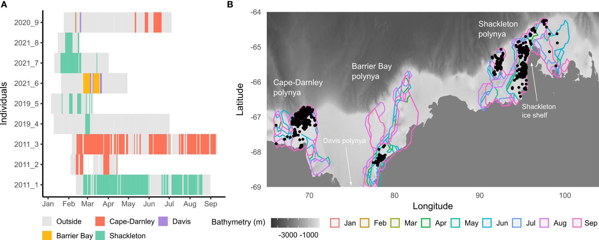
Figure 1 (A) shows polynya usage by 9 post-moult SES in 2011, 2019, 2020 and 2021 based on CTD positions associated to each profile (n = 2 292). All CTD positions were kept even if the recorded profiles had missing values. Each color is associated with a different polynya. (B) shows monthly contours for Cape-Darnley, Barrier Bay and Shackleton polynyas as well as the CTD profiles recorded within them (black points, n = 742). The monthly broadest contour among years between 2004 and 2019 was assigned for each polynya as explained in section 2.1. For all three polynyas, contours between January and March were the same as the one for April, which explains why they are not visible on the map. The bathymetry displayed on the map is based on the GEBCO data (2021). Note: polynyas contours are represented from January to September for all polynyas to show variations in extension, even if profiles were not recorded every month.

Individual seals were anesthetized with an intravenous injection of a 1:1 combination of tiletamine and zolazepam (Zoletil 100) (McMahon et al., 2000; Field et al., 2002) to attach the instrumentation. The data loggers were glued to the seals heads using quick-setting epoxy (Araldite AW 2101, Ciba; Field et al., 2012). Data on seal’s diving behavior as well as in situ hydrographic conditions were transmitted when the seal surfaces to breathe through communication with polar-orbiting Argos satellites (Harcourt et al., 2019).

The dataset is composed of in situ profiles of pressure, temperature, salinity and fluorescence. Fluorescence measurements are used as a proxy to estimate the concentration of chlorophyll-a in the water (Guinet et al., 2013). In this study, we have chosen not to convert chlorophyll-a fluorescence into chlorophyll-a concentration, as conversion ratios are highly variable in the Southern Ocean (Schallenberg et al., 2022), which could affect the validity of results interpretations. However, although quantitative assessments of phytoplankton biomass can hardly be reached with the sole use of fluorometers (Roesler et al., 2017; Petit et al., 2022), in vivo chlorophyll-a fluorescence is a commonly used method to detect presence of living phytoplanktonic organisms and study their dynamics in terms of concentration (IOCCG, 2011). The tag transmits an average of three profiles per day (3.3 ± 1.4) corresponding to the ascent phase of the deepest dives within 6-hour period. The data points transmitted for each CTD profile are a combination of temperature and salinity at a set of pre-selected standard depths and at another set of depths chosen by a broken-stick algorithm that selects the important inflection points in temperature and salinity data (recorded every second during the ascent phase of the dives) (Guinet et al., 2013).

The fluorometer tags deployed in 2011 sourced from Turner (Cyclops 7 model) and differed from those deployed since 2019 (Valeport, Hyperion model). The instruments differed primarily in their ability to detect low concentrations of chlorophyll-a: 0.03 μg.L^-1 compared with 0.066 μg.L^-1, respectively (Keates et al., 2020). The inter-tags variability is known to be non-negligible for both sensor’s models (Guinet et al., 2013; Keates et al., 2020; Le Ster et al., 2023) which implies caution when making quantitative comparisons of data.

All tags were calibrated in the laboratory and some of them were also tested at sea and compared to data collected by a ship-based CTD prior to deployment on individuals (Guinet et al., 2013). All tags were post-calibrated (Roquet et al., 2011; Roquet et al., 2014). Following data processing, the minimum accuracy was estimated to be 0.03°C and 0.05 psu. It could reach 0.01°C and 0.02 psu in the best cases. The marine mammal data were collected and made freely available by the International MEOP Consortium and the national programs that contribute to it¹.

Each profile of fluorescence, salinity and temperature had a vertical resolution of one meter after interpolation. No fluorescence data were available above 10 m and below 170 m. Profiles with missing values between these depth thresholds (10-170 m) were removed (n = 87 i.e, 10% of the profiles). The dataset for the nine individuals was then composed of 766 profiles recorded in polynyas (n = 300 in CDP, n = 398 in SP, n = 44 in Barrier Bay polynya and n = 24 in Davis polynya; Figure 1).

The mixed layer depth (MLD) was computed from temperature and salinity profiles using a density criteria ${\Delta }_{\rho }=0.03kg.m^{-3}$, with density at 10 m depth used as the reference value following de Boyer Montégut et al. (2004).

Fluorescence profiles can be corrected for non-photochemical quenching (NPQ) with a correction algorithm developed by Xing et al. (2018). The NPQ effect is induced by photo-inhibition in phytoplankton cells exposed to high light levels. This method aims at correcting the depression observed in the fluorescence signal (generally in the surface layer) resulting from the NPQ effect. As all profiles start at 10 m depth and the study focuses on autumn and winter, the effect of NPQ is negligible. However, when light was available, which is the case for profiles recorded in 2020 and 2021 (236 profiles out of 766), a correction was still applied. The correction is based on the definition of a “NPQ-layer”. Upper and lower boundaries are, respectively, the ocean surface, and the shallowest value between MLD and a light-threshold depth fixed at 15 μmol. m^-2s^-1 (PAR15, expressed in m). The maximum fluorescence value in the so-called NPQ-layer is then extrapolated up to 10 m depth which, as a result, discards the fluorescence depression due to NPQ (for details, see Xing et al. (2018)). Moreover, background noise from the fluorescence sensor detected at 170 m depth (where it is assumed that the fluorescence signal should be null) was removed from all the 766 fluorescence profiles.

The geographical positions transmitted via the Argos system uses the Doppler shift of the signal frequency received during the passing of one of the polar-orbitting satellites and depending on the position of the satellite relative to the transmitting tags, errors from 0.5 to 10 km may be observed. To provide the best location estimates we (i) filter the trajectories of individuals in order to (ii) interpolate the position of the CTD profiles from the filtered trajectory. The method used is based on a continuous-time state-space model presented in Jonsen et al. (2020) and implemented using the R package foieGras (now known as Animotum (Jonsen et al., 2019; Jonsen et al., 2020; Jonsen et al., 2023)).

Each profile was assigned to a broad regional area based on its location. These three areas: the continental shelf, the continental slope and the pelagic zone, were determined from the GEBCO_2021 Grided bathymetry (Gebco, 2021). The latitudinal limits of the continental slope were determined by graphic visualization every 0.5˚ longitudes (between -0.5˚E and 158°E) by plotting bathymetry against latitude. The beginning of the slope corresponds to the latitude where bathymetry starts to decrease drastically while the end of the slope corresponds to the first latitude where bathymetry is deeper than 2 900 m.

2.3 Water masses identification

Water masses within CDP and SP were identified following the criteria described in Table 1. Five main water masses known to be present in East Antarctica were considered as defined in Portela et al. (2021; 2022): Antarctic Surface Water (AASW), modified Circumpolar Deep Water (mCDW), Ice Shelf Water (ISW), Dense Shelf Water (DSW) and modified Shelf Water (mSW).

TABLE 1

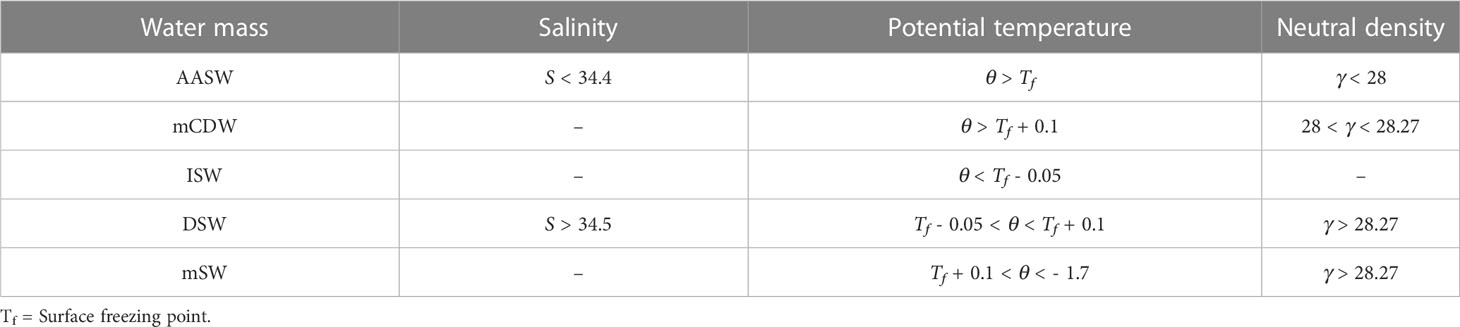
Table 1 Water masses criteria based on Portela et al. (2021).

2.4 Data analysis

A Principal Component Analysis (PCA) was used as an exploratory tool to identify the variability in the dataset and the underlying biological and physical patterns (Pauthenet et al., 2017). For CDP and SP, the 1-m interpolated temperature (T), salinity (S) and fluorescence (F) profiles between 10 and 170 m were used to build a matrix X of size N (rows) and L = 3(variables) × K (columns), with K (depths) = 161. Each row corresponds to an observation within polynyas and can be summarized by a vector p, such as:

$$p_n=(p_{n,1}^F,\dots ,p_{n,K}^F,p_{n,1}^S,\dots ,p_{n,K}^S,p_{n,1}^T,\dots ,p_{n,K}^T)$$

with $n=1,\dots ,N$. Each column of the matrix X corresponds to a record of one of the three variables: fluorescence, salinity and temperature between 10 and 170 m depth. The average profiles can be computed with:

$$\overline{p}=({\overline{p}}_1^F,\dots ,{\overline{p}}_K^F,{\overline{p}}_1^S,\dots ,{\overline{p}}_K^S,{\overline{p}}_1^T,\dots ,{\overline{p}}_K^T)$$

where ${\overline{p}}_k^i$, with $i\in \left\{F,S,T\right\}$ and $k=1,\dots ,\mathrm{ K}$, corresponds to the mean of the N coefficients of column k in X, i.e., ${\overline{p}}^i$ is the mean profile of fluorescence, salinity or temperature.

The aim is to compute a PCA on X (whose profiles are previously centered and reduced) which will provide two main results: the principal components (PCs) and the vertical modes of the profiles. The PCs correspond to the projection of the data onto the vertical modes. Vertical modes are used to identify the main variations in the profiles that explain the largest amount of variance in X and therefore extract the shape of the profiles according to the PCs:

$$\text{PCs }=X\times \Phi$$

$$\text{modes}={\overline{p}}^i\pm \sqrt{{\lambda }_l}{\Phi }_l$$

where $i\in \left\{F,S,T\right\}$ and ${\Phi }_l$ is the l^th eigenvector associated with the eigenvalue ${\lambda }_l$. The PCAs were performed using R version 4.1.1 (R Core Team, 2021).

3 Results

3.1 Seasonal signal of fluorescence within East Antarctic coastal polynyas

Mean monthly profiles of in situ fluorescence between February and September were used to describe the seasonal signal within polynyas (Figure 2). In February and March, CDP had weaker signals than SP (Figures 2A, B). For both polynyas, the fluorescence maximum in February is between the surface and about 25 m depth (Figures 2A, B). In February and March, the fluorescence signal becomes significantly lower at about 110 m in CDP and 125 m in SP (Figures 2A, B). In CDP, the MLD in February is just below the fluorescence maximum (Figure 2A) while it is at the maximum in SP (Figure 2B). A decrease of the fluorescence signal is observed in March for both polynyas and was accompanied by a deepening of the MLD when compared with February (Figures 2A, B). This fluorescence signal is mainly located above the MLD in CDP (Figure 2A), while the maximum of fluorescence is located at the depth level of the MLD in SP and a significant part of the fluorescence signal is present below the MLD (Figure 2B).

FIGURE 2

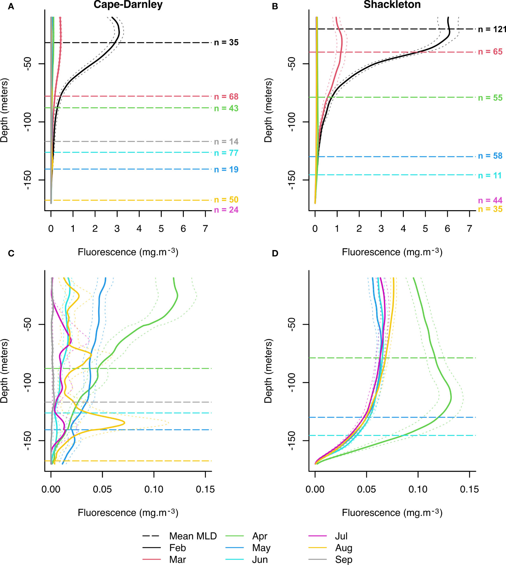
Figure 2 Mean fluorescence profiles between February and September for Cape-Darnley (A) and Shackleton (B) polynyas and associated standard errors (dotted line envelope). (C, D) are a magnification of (A, B) between April and September, respectively. The data were composed of a total of 330 and 432 fluorescence profiles for Cape-Darnley and Shackleton polynyas, respectively. If profiles presented missing values for some depth, there were ignored in the calculation of the mean and standard error. The dashed horizontal lines represent the mean mixed layer depth (MLD) for the corresponding months. MLDs that were outside the displayed depth range were not shown.

A magnification of the mean profiles for both polynyas between April and September (data ceased in August for SP) is presented in Figures 2C, D. Most of these profiles were recorded in 2011 (Figure 1A). A primary difference between the two polynyas is the shape of the mean profile in April which shows a fluorescence maximum (greater than 0.1 mg.m^-3) around 40 m depth for CDP (Figure 2C) compared with ~120 m depth for SP (Figure 2D). Surprisingly, the MLD is similar near 85 m depth between the two polynyas. A second difference is observed for the later profiles (between May and August). Fluorescence decreases with depth for SP (Figure 2D), while the mean profiles in CDP show some variation over depth with a maximum of fluorescence in August at around 130 m depth (Figure 2C). The MLD in August is also shallower for CDP (about 170 m) than for SP (about 240 m, not visible on the figure). All the fluorescence maxima observed during August within CDP were above the MLD, which is variable at this time of year (minimum of 53 m and maximum of 296 m). These fluorescence peaks were clearly evident in 7 profiles (out of 50 recorded in August in CDP) which showed a fluorescence value between 0.06 mg.m^-3 and 1.9 mg.m^-3 between 125 and 170 m depth (0.07 ± 0.04 mg.m^-3 at 135 m depth, Figure 2C) (Supplementary Figure S1). Three of these profiles are located on the slope, the others are on the shelf but in the vicinity of the slope (Supplementary Figure S1). Finally, we note that the fluorescence signal remains non-zero between May and August in both polynyas, despite some null fluorescence profiles and a weak signal (Figures 2C, D).

The monthly average profiles demonstrate that the fluorescence signal remains persistent until April in CDP and SP. The signal becomes weaker with time and deepens as does the MLD except for the SP in April where the fluorescence maximum is located below the MLD. CDP also showed an intriguing signal around 130 m depth in August in the vicinity of the continental slope.

3.2 Oceanographic conditions within East Antarctic coastal polynyas

The difference in the geographic distribution of profiles throughout the season between the two polynyas is illustrated in Figures 3A, B. Profiles within CDP are dispersed within the polynya with profiles on the continental slope and along the shelf throughout the season (Figure 3A). In SP, profiles at the beginning of the season (January-March) are mostly located within a cluster in the western part of the region (Figure 3B). Then, from April onwards, profiles are located along the ice shelf within two clusters distinguishing autumn profiles (April-June) from winter ones (July-August) (Figure 3B).

FIGURE 3

Figure 3 (A, B) show the geographic distribution of CTD-Fluo profiles colored by the day of the year for Cape-Darnley (n = 298) and Shackleton (n = 394) polynyas respectively. (C, D) represent the PC1/PC2 graphs for each polynya. The percentage of variance explained by each PC is specified in parentheses next to the axis labels. For illustration purposes, only the polynya’s contour for September is represented. The bathymetry displayed on the map is based on the GEBCO data (2021).

A PCA was performed on all fluorescence, temperature and salinity profiles for each polynya to identify the linkages between these variables (Figures 3C, D). Two and four profiles were removed as outliers for CDP and SP, respectively. The first three PCs represented around 77% of the variance for both polynyas. Figures 3C, D shows the first factorial plane associated with each polynya. The first component represents the seasonal effect for both polynyas: profiles early in the season are mainly on the negative side of the PC while profiles later in the season are on the positive side (Figures 3C, D). For SP, early profiles on the positive side of the first axis (yellow cluster, Figure 3D) correspond to profiles with near-zero fluorescence. Moreover, for both polynyas PC1 was correlated to the integrated fluorescence (i.e., the sum of the fluorescence along the water column), with a Pearson coefficient of 0.51 for CDP and 0.75 for SP, suggesting that integrated fluorescence is a good indicator of the seasonality of the fluorescence signal of the polynya. PC2 more likely represents spatial patterns (detailed in 3.2.1 and 3.2.2 below). The axes of the PCA were further explored through the examination of the relative contribution of the three observed variables (fluorescence, salinity and temperature) to the explained variance.

For both polynyas, Figure 4 shows for the three main PCs the percentage of variance explained by the 483 variables (3 (variables) × 161 (depths)) corresponding to fluorescence, salinity and temperature profiles at each depth from 10 to 170 m. As each variable has an associated depth, it is possible to reconstruct an “axis contribution profile” for fluorescence, salinity and temperature for each PC. For each variable, fluorescence, salinity or temperature, the sum of the explained variance at each depth corresponds with the variance explained by this given variable. When the explained variance is zero at certain depths for a given variable, then the vertical modes associated with this variable (Figures 5, 6) are not interpretable at that depth specifically. For CDP, the variance of the axis between 0 and 70 m depth on PC1 is mostly explained by salinity (red curve, Figure 4A). From 100 m depth, temperature and salinity explain almost all the variance of this axis (blue and red curves, Figure 4A). For PC2, temperature and fluorescence co-vary together since they explain an equivalent share of variance along the profile and are opposite to salinity (Figure 4B). A shift occurs around 60 m depth where salinity starts to explain the majority of the variance of the axis while temperature and fluorescence explain the variance nearer the surface (Figure 4B). The variance of PC3 is almost entirely explained by fluorescence (green curve, Figure 4C). In SP, fluorescence and temperature co-vary together on the first two PCs (blue and green curves, Figures 4D, E). PC1 is mainly explained by these two variables from the surface to depth while salinity explains almost all the variance of PC2 (Figures 4D, E). The variance of PC3 is mainly explained at the surface by salinity (from 10 m to 50 m depth) while fluorescence explains almost all the variance from 100 m depth (Figure 4F). Thus, PC3 discriminates the rare fluorescence profiles presenting a high signal at depth from those with no signal.

FIGURE 4

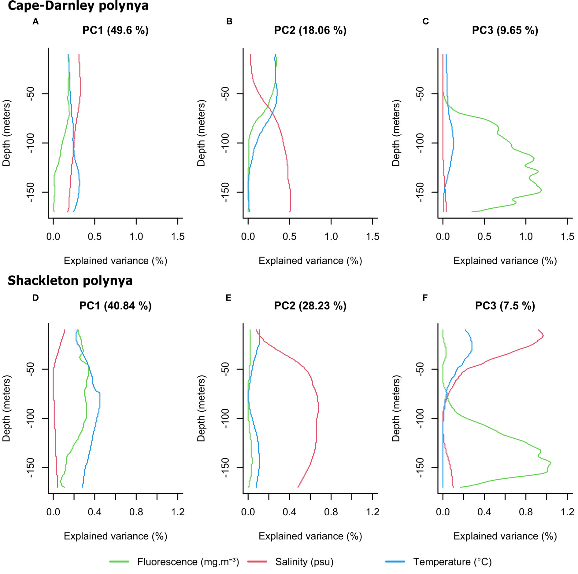
Figure 4 Variance explained by the fluorescence, salinity and temperature variables of the PCA for Cape-Darnley (A–C), (n = 298) and Shackleton (D–F), (n = 394) polynyas for the three main PCs. The percentage of variance explained by each PC is specified in parentheses in the titles. Note for each variable (fluorescence, salinity or temperature), the sum of the explained variance every meter corresponds to the variance explained by the variable.

FIGURE 5

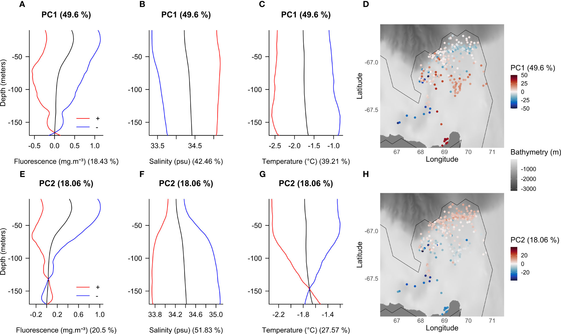
Figure 5 Vertical modes from the first (A–C) and second (E–G) PC and their spatial distributions (D, H) for the PCA based on Cape-Darnley polynya fluorescence, salinity and temperature data. The colored curves show the mean profile (black) and the effects of adding (red) or subtracting (blue) eigenvectors. The percentage of variance explained by each PC is specified in parentheses next to titles. The percentage of variance explained by each variable is specified in parentheses next to axis labels. The zero value on the map (white color) corresponds to the mean profile. For illustration purposes only the polynya’s contour for September is represented. The bathymetry displayed on the map is based on the GEBCO data (2021). Note: the red and blue curves show the direction of the effects of adding and subtracting each principal component curve to the mean, the amplitude is not respected (hence some unphysical values such as negative fluorescence). Ramsay and Silverman (2005) indicates that a suitable multiple of the PCs can be used to give easily interpretable results.

FIGURE 6

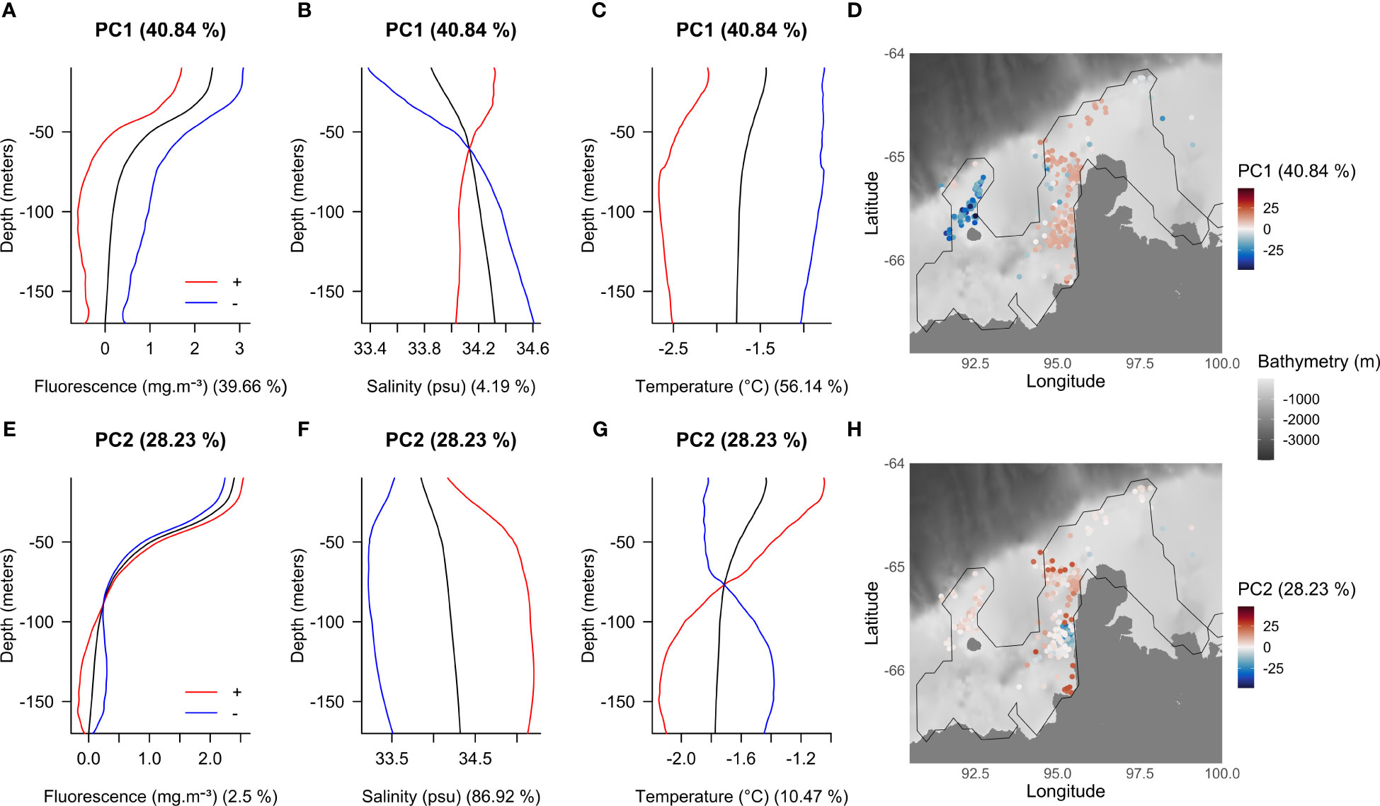
Figure 6 Vertical modes from the first (A–C) and second (E–G) PC and their spatial distributions (D, H) for the PCA based on Shackleton polynya fluorescence, salinity and temperature data. The colored curves show the mean profile (black) and the effects of adding (red) or subtracting (blue) eigenvectors. The percentage of variance explained by each PC is specified in parentheses next to titles. The percentage of variance explained by each variable is specified in parentheses next to axis labels. The zero value on the map (white color) corresponds to the mean profile. For illustration purposes only the polynya’s contour for September is represented. The bathymetry displayed on the map is based on the GEBCO data (2021). Note: the red and blue curves show the direction of the effects of adding and subtracting each principal component curve to the mean, the amplitude is not respected (hence some unphysical values such as negative fluorescence). Ramsay and Silverman (2005) indicates that a suitable multiple of the PCs can be used to give easily interpretable results.

The PCA identifies that fluorescence and temperature tend to co-vary together (except for the PC1 in CDP) and have a similar contribution in explaining the profile patterns observed in both CDP and SP. Moreover, their contribution is commonly opposing that of salinity. Interestingly, fluorescence explains almost all the variability of PC3 at depth for both polynyas.

The objective then is to identify the spatial and temporal variations in fluorescence, salinity and temperature for these two polynyas and to determine their drivers by the analysis of the vertical modes from the PCA. In the following sections, results are presented separately for each of the two polynyas. Following Ramsay and Silverman (2005), Figures 5, 6 present the effect of adding (red curve) or subtracting (blue curve) the first and second modes to the mean fluorescence, salinity and temperature profiles for CDP and SP, respectively.

3.2.1 Cape-Darnley polynya

PC1 summarizes almost 50% of the variance and reflects the seasonality (Figure 3C). Thus, red curves (positive side of the PC1) for each variable provide information on the shape of profiles later in the season (i.e., during winter) (red curves, Figures 5A–C). PC1 indicates that in winter compared to summer, there is less fluorescence than average and waters are saltier and colder from the surface to 170 m depth (red curves, Figures 5A–C). The opposite is observed for profiles earlier in the season (blue curves, Figures 5A–C). As the profiles were well dispersed within the polynya throughout the season (Figure 3A), no clear spatial pattern is observed for PC1 (Figure 5D).

For PC2, we observed two main clusters on the map: the profiles located on the continental slope (red points) and those located on the continental shelf (blue points) (Figure 5H). This PC is likely associated with the bathymetry. These two clusters suggest differences in environmental conditions between these two areas. The continental slope is characterized by lower salinity over the entire water column and associated with colder temperatures and less fluorescence from the surface to about 140 m depth compared to the continental shelf (red curves, Figures 5E–G). Below 140 m the temperature and fluorescence become higher than the average profile (red curves, Figures 5E, G) but these two variables do not explain any variance of PC2 at this depth (Figure 4B), making this observation uninterpretable. The continental shelf is therefore characterized by saltier and warmer waters throughout the upper water column compared with the continental slope and associated with higher fluorescence down to 140 m (blue curves, Figures 5E–G). There is also a near-surface pattern observed in the salinity and temperature signals to about 60 m at both locations: on the shelf, surface salinity is lower and temperature is higher than at depth, while both remain higher than profiles on the slope (Figures 5F, G).

3.2.2 Shackleton polynya

For this polynya, the non-homogeneous distribution of the profiles during the season (Figure 3B), means that geographical and temporal effects cannot be distinguished.

However, as described for CDP, PC1 (Figure 3D) seems to represent the seasonality with the mapped PC1 (Figure 6D) reflecting the same spatiotemporal clusters identified in Figure 3B. Likewise, profiles later in the season (i.e., in winter) are associated with less fluorescence and colder temperatures up to 170 m depth compared with the average profile (red curves, Figures 6A, C). Unlike CDP, the water is saltier down to 60 m and then becomes fresher than the average from 60 m to 170 m depth (red curve, Figure 6B). However, the salinity represents less than 5% of the variance of the axis (Figure 4D). The opposite is observed for profiles earlier in the season (blue curves, Figures 6A–C).

For PC2, salinity explains more than 85% of the variance (Figure 4E). This PC discriminates a specific area close to the ice shelf (blue points, Figure 6H) characterized by low salinity over the entire water column compared to the rest of the polynya (blue curve, Figure 6F). It is also associated with warmer temperatures from about 75 m to 170 m depth compared with the rest of the polynya (blue curve, Figure 6G). Fluorescence explains less than 3% of the variance of the axis (Figure 4E). It is globally stronger at the surface than at depth but varies little between the two zones discriminated by the PC except for a slight peak around 130 m depth for those profiles in the ice shelf vicinity (blue curve, Figure 6E). This finding corresponds with the peak of fluorescence observed at depth in the average April profiles presented in Figure 2D.

A more detailed investigation of the temperature and salinity profiles located in the specific ice shelf area described above is presented in Figure 7. When classifying the profiles according to the day of the year, we can observe a change towards warmer temperatures at depth over time (Figure 7B). The profiles are also saltier at depth (below about 100 m) compared with the surface but remain generally fresher than the profiles located in the rest of the polynya (Figures 7A, 6F).

FIGURE 7

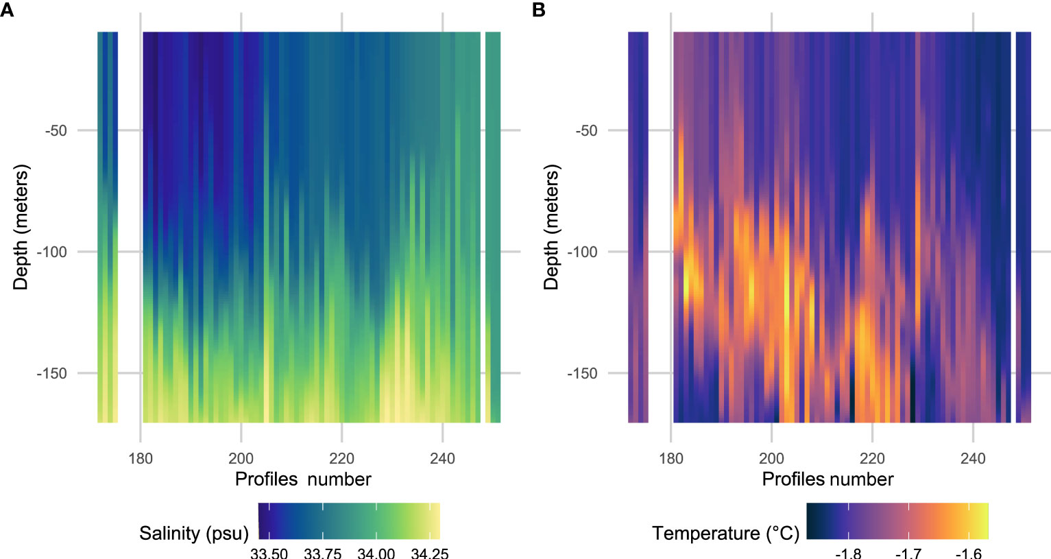
Figure 7 Salinity (A) and temperature (B) profiles observed in the area next to the ice shelf in Shackleton polynya discriminate by the negative PC2 for this polynya (n = 75, see blue points in Figure 6H). The profiles are ordered according to the day of the year (from day 80 to 122 i.e., in April) but the profile number is represented on the x-axis as some profiles were registered on the same day. Note: blanks between profiles correspond to days without data.

PCA results demonstrate that temperature and salinity (to a lesser extent for SP) have a strong impact on the seasonal fluorescence signal in the two polynyas studied (PC1 represent more than 40% of the variance of the signals for both polynyas). However, other factors such as topography or the presence of an ice shelf also seem to play an important role on the distribution and amplitude of the fluorescence signal in the water column.

3.3 Water masses: temporal and vertical distribution

Water masses were identified for CDP (Tables 2, 3; Supplementary Tables S1, S2) and SP (Table 4; Supplementary Table S3). For both polynyas, the percentage of each water mass within a period of time and a depth interval was computed in order to link these results with those from the PCA analyses (Supplementary Tables S1–S3). For clarity, only the dominant water masses are presented in Tables 2–4.

TABLE 2

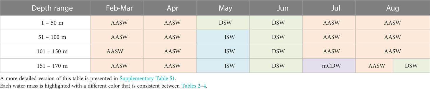
Table 2 Main water masses identified within Cape-Darnley polynya on the shelf.

TABLE 3

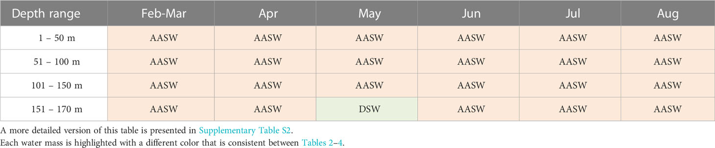
Table 3 Main water masses identified within Cape-Darnley polynya on the slope.

TABLE 4

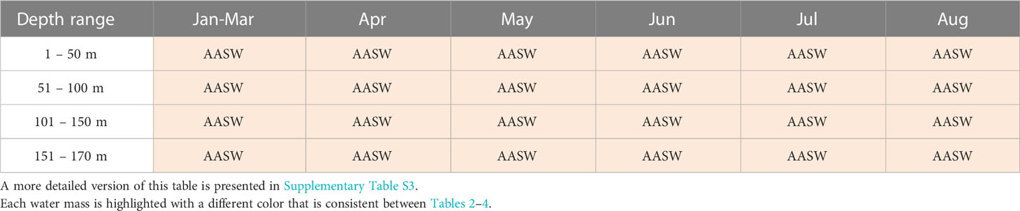
Table 4 Main water masses identified within Shackleton polynya.

The CDP and SP are unique in terms of dominant water masses. Concerning CDP, a distinction between the continental shelf (Table 2) and slope (Table 3) was made due to the spatial distribution of the profiles. On the continental shelf (Table 2), AASW dominates between February and April from the surface to 170 m depth. Then during May, DSW dominates at the surface while ISW has the highest proportional contribution between 51 to 170 m depth. DSW is predominant in June. In July, ASSW is present up to 150 m depth while mCDW dominates between 151 m and 170 m depth. ASSW has the highest proportional contribution in August down to 170 m depth and is proportionally similar to DSW below 151 m depth. On the continental slope in CDP, AASW is predominant between February and August throughout the upper water column, except in May between 151 and 170 m depth where DSW has the highest proportion (Table 3). SP, in contrast, is dominated by AASW from the surface to 170 m depth for the whole observation period between January and August (Table 4; Supplementary Table S3).

4 Discussion

We present the first chlorophyll fluorescence signals recorded from in situ biotelemetry data in East Antarctic coastal polynyas during the austral autumn and winter. We identified differences in the amplitude and persistence of the fluorescence signal through the season between CDP and SP (Figure 2). We observed a significant fluorescence signal persisting through autumn (until April) in both polynyas with an additional small but persistent signal arising in winter (August) for the CDP along the continental slope. This fluorescence signal, a proxy for chlorophyll-a concentration, may have important ecological implications regarding trophic cascades through the autumn/early winter. Using PCA as an exploratory analysis, we described the seasonal cycle of fluorescence and identified how temperature and salinity were associated with patterns of fluorescence for each polynya. We found that fluorescence was positively associated with warmer waters in both polynyas and with fresher waters in CDP through the whole period (February to August) (Figures 5A–C, 6A–C). By zooming in on the role of sea-floor topography for CDP, we observed colder and fresher waters associated with poorer fluorescence on the slope compared to the continental shelf (Figures 5E–H). In SP, warm and fresh waters at depth (from 75 to 170 m depth) in the immediate vicinity of the ice shelf between late March and early April were associated with a weak, but noteworthy, peak of fluorescence below the MLD (Figures 6E–H). This peak in fluorescence may be associated with the intrusion of warm waters which likely leads to the melting of the ice shelf and, in turn, can have implications via iron input for stimulating a slight phytoplankton growth (St-Laurent et al., 2017). A detailed discussion follows and all the hypotheses developed are illustrated in Figure 8.

FIGURE 8

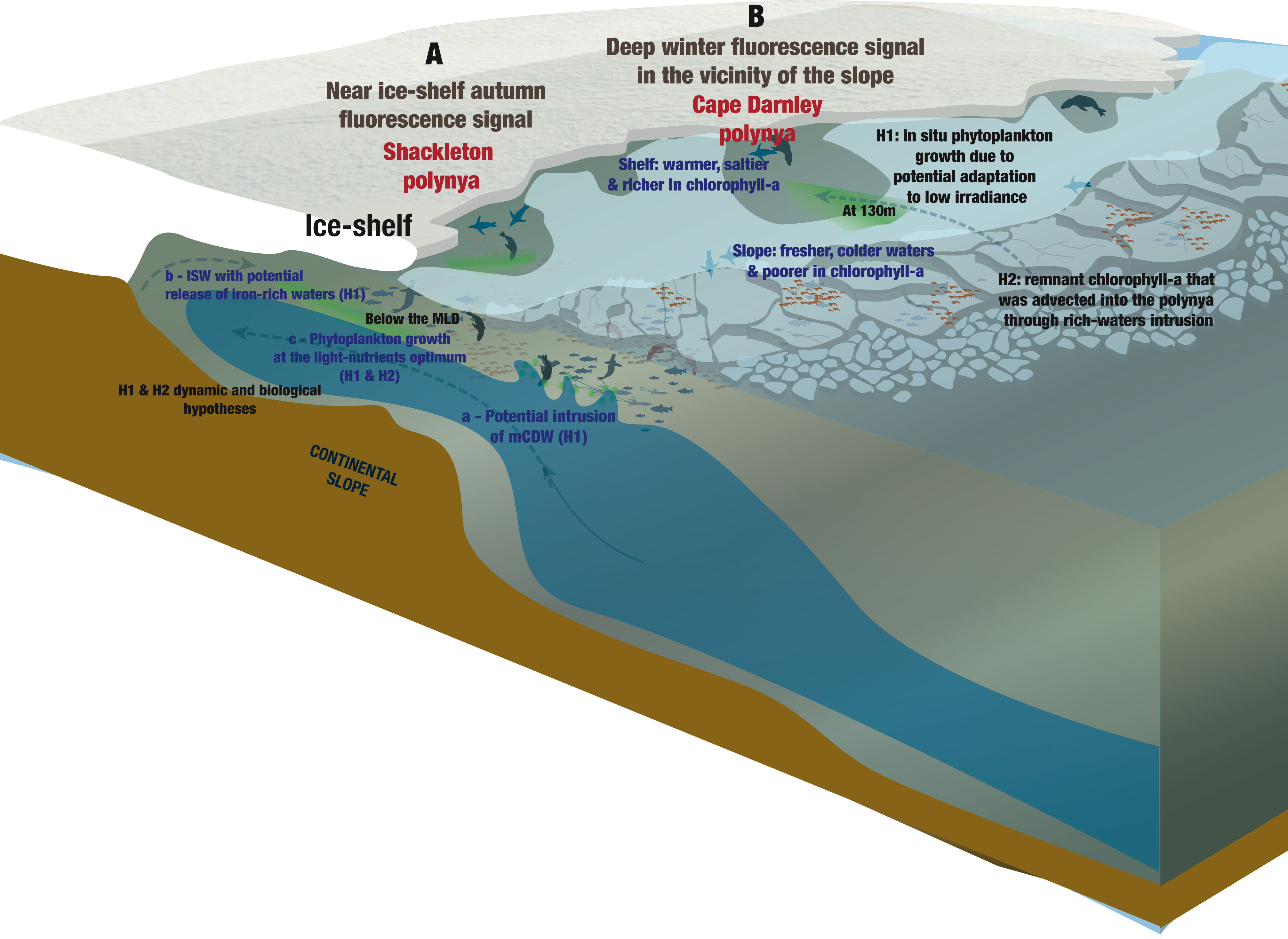
Figure 8 Illustration of the results and hypotheses developed in this study in order to provide potential explanation on the observed (A) near ice-shelf autumn (April) fluorescence signal within Shackleton polynya and the (B) deep winter (August) fluorescence signal within Cape-Darnley polynya. The illustration was made by S. Labrousse using Adobe Illustrator.

4.1 Florescence signal within polynyas and associated oceanographic conditions

The fluorescence signal persisted until April within CDP and SP (Figures 2C, D), hence there is a strong evidence for the presence of chlorophyll-a and thus phytoplankton biomass during the Austral autumn. These fluorescence signal detections until early autumn within the sea ice region has rarely been observed and documented (Lieser et al., 2015) and, until now, has not been demonstrated with in situ observations. This study provides the first description of these new in situ CTD-fluorescence data within polynyas. The differences in amplitude of the fluorescence signals between the two polynyas (Figures 2A, B) is likely partly due to differences in the sensors’ characteristics (including sensitivity and calibration coefficients) given the two different sensors used over the life of the study (see detailed explanation in section 2.2). While sensors particularities may explain some of the differences, environmental conditions will no doubt also contribute to some of the differences we observed. Indeed, each polynya is unique in several aspects including physical location (for example CDP straddles the continental shelf and slope while SP is in the vicinity of the ice shelf), oceanographic conditions, and thus biological activity (Smith and Barber, 2007).

The fluorescence signal was still present in some profiles from May to August in both polynyas, despite the low amplitude of the signal (Figures 2C, D). This can reflect a background chlorophyll-a concentration that remains through winter. Fritsen et al. (2008) demonstrated that exchanges between the water column and sea ice can persist over winter, and if the sea ice is filled with algal cells, then these could be released into the water column over winter, explaining a weak but persistent fluorescence signal across the months.

The seasonal decrease in fluorescence signal was associated with colder and saltier waters for CDP (Figures 5A–C) and with colder waters for SP (Figures 6A–C). Several factors could contribute to the attenuation and deepening of the signal such as the availability of light, dilution, iron limitation and grazing (Wright et al., 2010; Lieser et al., 2015). In autumn, atmospheric cooling drives sea ice production and significant salt release; combined with the strengthening of the winds in autumn and winter, it leads to a de-stratification of the water column and a thickening of the surface layer (Behera et al., 2020) limiting light availability for phytoplankton cells.

4.1.1 Cape-Darnley polynya

4.1.1.1 Winter fluorescence signal

Despite the decline of the fluorescence signal during winter, a non-negligible fluorescence signal around 130 m depth was observed in August in CDP along the slope (Figure 2C; Supplementary Figure S1). These profiles (n = 50) were checked individually to prevent outliers. Seven of them had a shape consistent with the MLD, with a signal between 0.06 mg.m^-3 and 1.9 mg.m^-3 above the MLD (average of 0.07 ± 0.04 (SD) mg.m^-3 at 135 m depth, Figure 2C), while the other profiles (n=43) were close to zero (Supplementary Figure S1). This unexpected result raises new questions about the possibility of such fluorescence signal appearing or being maintained at this depth during the austral winter. With these observations, it is impossible to know whether the signal corresponds to an i) in situ phytoplankton growth or to ii) remaining chlorophyll-a from phytoplankton cells that would have been maintained through the winter. Different hypotheses are suggested below, depending on the interpretation considered, attempting to explain the deep fluorescence signal observed in August in CDP (Figure 8B).

If we consider that the fluorescence signal is incipient, i.e. coming from in situ phytoplankton growth, one possible explanation for the observation of a deep winter fluorescence signal may be associated with the adaptation of phytoplankton to low irradiance conditions (Figure 8B). Hague and Vichi (2021) posited that phytoplankton can be present around 100 m depth in August around 65˚S in a situation where the MLD is deeper than 100 m and sea ice is still strongly present. The case of polynyas is not mentioned in this study but the authors suggest that the adaptation of Antarctic phytoplankton to low irradiance is probably underestimated and that the observation of chlorophyll-a peaks in August may support this theory. Laboratory experiments and in situ observations have also demonstrated the surprising adaptation of phytoplankton species, including diatoms, to the low light, iron and temperature conditions of the Southern Ocean (Joy-Warren et al., 2019; Strzepek et al., 2019). These observations support the feasible early appearance of a fluorescence signal in the CDP before the end of winter.

This deep fluorescence signal could also be explained by the second hypothesis i.e., a remnant signal during the winter and not an in situ growth (Figure 8B). The observations indicate that the fluorescence signal is stronger in August rather than in June or July (Figure 2C); this suggests that a process has taken place in August. We hypothesize that the advection of chlorophyll-a (when loss rate is low e.g., grazing) from another source than the polynya could explain the origin of this deep winter fluorescence signal. The presence of mCDW and DSW on the continental shelf at the same depths in July and August, respectively (Table 2), could demonstrate an advection of water into the polynya that could be rich in chlorophyll-a, explaining the deep fluorescence signal observed. As no fluorescence signal was observed in September in CDP (Figure 2C) this suggests that the deep fluorescence signal in August was ephemeral and therefore rather advected than growing. If the signal corresponded with in situ phytoplankton growth, we would expect to see a stronger signal in September in this same polynya, which is not the case. However, the few data recorded in September (n = 14) limits our interpretation.

Our CDP findings can support the idea that polynyas may be biologically active throughout most of the year, and have an ecological importance for the Antarctic ecosystems up to higher trophic levels (Karnovsky et al., 2007). Although the winter fluorescence signal was not observed in the SP, observations in CDP suggests that under favorable conditions (hypothetically: long surface residence time, nutrient- and iron-rich waters, stratified water column or advection of chlorophyll-a-rich waters) a fluorescence signal is possible in other polynyas. However, more data is needed to confirm these observations and identify the drivers of winter fluorescence signal.

4.1.1.2 Comparison of the signal between the continental shelf and slope

We found clear oceanographic differences in conditions on the continental shelf compared with the continental slope within CDP (Figures 5E–H). On the continental slope, the water was generally fresher, colder and had lower fluorescence signals (Figure 8B). This is an important finding given the current lack of knowledge about biological productivity within these two areas, particularly the continental slope. The continental slope is relatively narrow and difficult to access especially at the onset of autumn and winter, and consequently poorly studied with large knowledge gaps remaining (Heywood et al., 2014; Thompson et al., 2018). These findings provide the information that CDP has more fluorescence on the shelf than on the slope from February to September. This result is also reflected by the presence of nutrient-rich water masses on the continental shelf from May onwards to August with notably ISW, DSW and mCDW (Table 2) (Prézelin et al., 2000; Herraiz-Borreguero et al., 2016) while the slope is predominantly composed of AASW between the surface and 170 m depth between February and August (Table 3).

4.1.2 Shackleton polynya

In the SP, salinity have an important spatial variability as it accounts for more than 85% of the variance of PC2 (Figure 4E) and highlights a low-salinity area near the ice shelf in April from the surface to 170 m depth (Figures 6E–H). On Figure 4E, we observe that temperature and fluorescence both share a low but non negligeable part of the variance below 100 m depth, making the interpretation of these modes noteworthy. Consequently, the low-salinity waters near the ice shelf were associated with a higher-than-average fluorescence signal and warmer-than-average water from about 75 m depth to 170 m compared to profiles from elsewhere in the polynya (Figures 6E–H). By carefully assessing the fluorescence profiles recorded in this area individually, we found that 46% of them had a fluorescence signal below the MLD that was greater than 0.12 mg.m^-3 and were recorded between the end of March and April, contributing to the subsurface fluorescence maxima observed in the average April profiles (Figure 2D). During the mixing of the water column, the fluorescence peak is expected to remain above the MLD rather than below (Gu et al., 2020; Prakash et al., 2020; Louw et al., 2022). Two hypotheses, not mutually exclusive, might explain the phenomenon observed in SP: the dynamic hypothesis centered around the physical structure; and the biological hypothesis which focuses on the biological activity and vertical movement of phytoplankton (Figure 8A).

The dynamic hypothesis suggests that the freshening observed in SP nearby the ice shelf could correspond with an intrusion or advection of warm water, melting the ice shelf and thereby increasing freshwater inputs and stratifying the water column (i.e., shallower MLD) (Figure 8A). Our observations confirm that water is saltier (Figure 7A) and warmer (Figure 7B) at depth within this area compared to the surface. Indeed, the fresh melt-waters, less dense, may rise to the surface, explaining the saltier waters at depth. This dynamic hypothesis of ice shelf melting by warmer waters is supported by the study of Rignot et al. (2013) in which the authors observed high ice shelf melting rate from basal melting in SP. Also, the study by St-Laurent et al. (2017) demonstrated that ice shelf melting represents a non-negligible input of iron contributing to primary production during summer in the Amundsen Sea polynya (Antarctica). The melting of the Shackleton ice shelf could thus represent an iron supply supporting the growth of phytoplankton, explaining the maximum of fluorescence we observed below the MLD. Although the analysis of the water masses within the polynya reveals that AASW is clearly dominating in the upper 170 m from April onward (Table 4), we observed from 100 to 170 m some presence of ISW and mCDW (warm water) between January and February (e.g., more than 15% of ISW in January below 100 m depth) (Table 4; Supplementary Table S3). mCDW could then be responsible for the melting of the ice shelf providing ISW and iron input feeding the fluorescence signal observed a few weeks later, in April, at the same depths. However, it is important to highlight two main points in order to explain why we do not observe mCDW in April and only a slight signal in January and February: first, we hypothesize that mCDW may be located deeper than 170 m (Portela et al., 2022) and therefore could melt the ice-shelf deeper; second, high quantity of AASW can also prevent the detection of any intrusion of mCDW in March-April as it mixes with dominant fresh waters.

The biological hypothesis is based on the study of Gu et al. (2020) in autumn-winter-spring during which the MLD appears to govern the depth of the chlorophyll-a maximum but in summer the relationship is less clear with occasional chlorophyll-a peaks below the MLD (Figure 8A). Gu et al. (2020) hypothesized that during summer, access to nutrients controls most of the vertical distribution of chlorophyll-a. Indeed, at this time of the year, when the water column is highly stratified (i.e. a shallow MLD), the supply of nutrients by upwelling is low (Behera et al., 2020). Thus, surface nutrient stocks can be depleted. If this occurs, species that can control their buoyancy, such as large diatoms (Baldry et al., 2020), may tend to descend below the MLD to find an optimum between light and nutrients. In our case, the presence of non-negligeable fluorescence signal below the MLD may be associated with large phytoplankton moving to areas within the water column where light and nutrient supply are optimized.

The two suggested hypotheses may be related: ice shelf melting would lead to a supply of iron necessary for the growth of phytoplankton and diatoms (Ryan-Keogh and Smith, 2021) in the same way that it would tend to stabilize the water column by the supply of fresh water (Figure 8A). Thus, the species with the ability to control their buoyancy might over time be attracted deeper, below the mixed layer, to find richer waters, possibly explaining the fluorescence signal observed around 130 m depth near the ice shelf in the SP in April. This explanation is supported by Cullen (2015) who noted that depth of the subsurface biomass maximum layer is close to the boundary between the nutrient-limited layer and the light-limited layer.

It is important to emphasize that this work has focused on the linkages between fluorescence, temperature and salinity but other drivers, such as light, nutrients, grazing, and currents, may also be involved in the genesis and maintenance of the fluorescence signal. Unfortunately, such data are currently unavailable within polynyas due to the difficulty to sample these regions in autumn and winter and will not be discussed in the present research.

This study focuses on two polynyas: the Cape Darnley polynya, which straddles the continental shelf and slope, and is known to be a major source of Antarctic bottom water through the Cape-Darnley Bottom Water with an impact on the overturning circulation (Ohshima et al., 2013); and the Shackleton polynya which is located in the immediate vicinity of the Shackleton ice shelf. As described previously, both presented intra-polynya spatial and temporal differences in terms of fluorescence, temperature and salinity. These two polynyas differ in terms of water masses and geographical location, however they both show biological activity throughout the year, underlining their potential importance for Antarctic ecosystems. These new results do not provide information on whether the patterns described can be generalized or applicable to all polynyas. Nevertheless, they encourage further studies throughout the year to be able to increase the current first observations and understand the biological role of Antarctic polynyas.

4.2 Conclusions

The description of the water column fluorescence signal within polynyas and the identification of the related environmental conditions greatly increased our knowledge of the important, yet highly inaccessible, Antarctic coastal polynyas. Indeed, the persistence of the signal until April with the possibility of a signal during August highlights the potential ecological attractiveness of polynyas. In addition, this study provides evidence on the influence of topography on the attenuation and deepening of the fluorescence signal in CDP and suggests potential drivers of the fluorescence signal, poorly observed, such as ice shelf melting as a possible iron source and the potential effect of the physiology/ecology of some phytoplankton species contributing to unsuspected adaptations (potential control of their buoyancy and adaptation to low light environments). Since this study uses data collected by SES that may exhibit variable behavior depending on their habitat, the next challenge will be to study the effect of this fluorescence signal on SES foraging behavior. Our results demonstrate the utility of animal-borne fluorometer-CTDs and highlight the need to continue such deployments over the long-term to capture the inherent variability in these complex and remote ecosystems.

Data availability statement

Publicly available datasets were analyzed in this study. These data can be found here: https://www.meop.net/database/meopdatabases/ in the MEOP-CTD database section. All data, codes, and materials used in the analyses are available on a Dryad repository: doi:10.5061/dryad.wstqjq2rd.

Ethics statement

The animal study was reviewed and approved by The Australian Antarctic program, The University of Tasmania and The Terres Australes et Antarctiques Françaises.

Author contributions

LB, SL, SJ, and EPau conceptualized the study, and the methodology was put in place by LB, SL, EPau, EPor, and LLS. The analyses were run by LB and EP. The seal dataset was collected and assembled by BP, J-BS, CM, RH, MH, CG, SB, and J-BC. AD, SJ, and SL worked on the funding acquisition and project administration. LB wrote the first draft of the manuscript with the help of SL, and all authors contributed substantially to revisions. All authors approved the submitted version.

Funding

This project was supported by NASA award No 80NSSC21K1132 and NASA award No 80NSSC20K1289. The seal CTD-SRDL tags and deployments were funded and supported through a collaboration between the Centre d’Etudes Biologiques de Chizé, the University of Tasmania and the Integrated Marine Observing System (IMOS). The data acquisition of this project was financially and logistically supported by the French Polar Institute (program 109: PI. C. Barbraud and 1201: PI. C. Gilbert and C. Guinet), SNO-MEMO, CNRS and CNES-TOSCA and IMOS. IMOS is enabled by the National Collaborative Research Infrastructure Strategy (NCRIS). It is operated by a consortium of institutions with the University of Tasmania as Lead Agent (https://imos.org.au/). The Australian Research Council provided financial support through Discovery Project DP180101667 and this work also represents a contribution to DP230101368.

Acknowledgments

We wish to thank all the people who contributed to the tag deployments and recoveries in the field through the whole duration of this study. AD, SJ, LB, and SL acknowledge NASA award No 80NSSC21K1132. KK acknowledges NASA award number 80NSSC20K1289. Any opinions, findings, and conclusions or recommendations expressed in this material are those of the author(s) and do not necessarily reflect the views of the National Aeronautics and Space Administration.

Conflict of interest

The authors declare that the research was conducted in the absence of any commercial or financial relationships that could be construed as a potential conflict of interest.

Publisher’s note

All claims expressed in this article are solely those of the authors and do not necessarily represent those of their affiliated organizations, or those of the publisher, the editors and the reviewers. Any product that may be evaluated in this article, or claim that may be made by its manufacturer, is not guaranteed or endorsed by the publisher.

Supplementary material

The Supplementary Material for this article can be found online at: https://www.frontiersin.org/articles/10.3389/fmars.2023.1186403/full#supplementary-material

Footnotes

1. ^ http://www.meop.net

References

Arce F., Hindell M. A., McMahon C. R., Wotherspoon S. J., Guinet C., Harcourt R. G., et al. (2022). Elephant seal foraging success is enhanced in Antarctic coastal polynyas. Proc. R. Soc. B: Biol. Sci. 289, 20212452. doi: 10.1098/rspb.2021.2452

CrossRef Full Text | Google Scholar

Arrigo K. R., van Dijken G. L. (2003). Phytoplankton dynamics within 37 Antarctic coastal polynya systems. J. Geophys. Res. 108. doi: 10.1029/2002JC001739

PubMed Abstract | CrossRef Full Text | Google Scholar

Arteaga L. A., Boss E., Behrenfeld M. J., Westberry T. K., Sarmiento J. L. (2020). Seasonal modulation of phytoplankton biomass in the Southern Ocean. Nat. Commun. 11, 5364. doi: 10.1038/s41467-020-19157-2

PubMed Abstract | CrossRef Full Text | Google Scholar

Bailleul F., Charrassin J.-B., Ezraty R., Girard-Ardhuin F., McMahon C. R., Field I. C., et al. (2007). Southern elephant seals from Kerguelen Islands confronted by Antarctic Sea ice. Changes in movements and in diving behaviour. Deep Sea Res. Part II: Topical Stud. Oceanogr. 54, 343–355. doi: 10.1016/j.dsr2.2006.11.005

CrossRef Full Text | Google Scholar

Baldry K., Strutton P. G., Hill N. A., Boyd P. W. (2020). Subsurface chlorophyll-a maxima in the Southern Ocean. Front. Mar. Sci. 7. doi: 10.3389/fmars.2020.00671

CrossRef Full Text | Google Scholar

Barber D. G., Massom R. A. (2007). “Chapter 1 the role of sea ice in Arctic and Antarctic Polynyas,” in Elsevier Oceanography Series (Elsevier) 74, 1–54.

Google Scholar

Behera N., Swain D., Sil S. (2020). Effect of Antarctic sea ice on chlorophyll concentration in the Southern Ocean. Deep Sea Res. Part II: Topical Stud. Oceanogr. 178, 104853. doi: 10.1016/j.dsr2.2020.104853

CrossRef Full Text | Google Scholar

Blain S., Renaut S., Xing X., Claustre H., Guinet C. (2013). Instrumented elephant seals reveal the seasonality in chlorophyll and light-mixing regime in the iron-fertilized Southern Ocean. Geophys. Res. Lett. 40, 6368–6372. doi: 10.1002/2013GL058065

CrossRef Full Text | Google Scholar

Boehme L., Lovell P., Biuw M., Roquet F., Nicholson J., Thorpe S. E., et al. (2009). Technical Note: Animal-borne CTD-Satellite Relay Data Loggers for real-time oceanographic data collection. Ocean Sci. 5, 685–695. doi: 10.5194/os-5-685-2009

CrossRef Full Text | Google Scholar

Charrassin J.-B., Hindell M., Rintoul S. R., Roquet F., Sokolov S., Biuw M., et al. (2008). Southern Ocean frontal structure and sea-ice formation rates revealed by elephant seals. Proc. Natl. Acad. Sci. 105, 11634–11639. doi: 10.1073/pnas.0800790105

CrossRef Full Text | Google Scholar

Cullen J. J. (2015). Subsurface chlorophyll maximum layers: enduring enigma or mystery solved? Annu. Rev. Mar. Sci. 7, 207–239. doi: 10.1146/annurev-marine-010213-135111

CrossRef Full Text | Google Scholar

de Boyer Montégut C., Madec G., Fischer A. S., Lazar A., Iudicone D. (2004). Mixed layer depth over the global ocean: An examination of profile data and a profile-based climatology. J. Geophys. Res.: Oceans 109. doi: 10.1029/2004JC002378

CrossRef Full Text | Google Scholar

Field I. C., Harcourt R. G., Boehme L., Bruyn P.J.N.d., Charrassin J.-B., McMahon C. R., et al. (2012). Refining instrument attachment on phocid seals. Mar. Mammal Sci. 28, E325–E332. doi: 10.1111/j.1748-7692.2011.00519.x

CrossRef Full Text | Google Scholar

Field I. C., McMahon C. R., Burton H. R., Bradshaw C. J. A., Harrinigton J. (2002). Effects of age, size and condition of elephant seals (Mirounga leonina) on their intravenous anaesthesia with tiletamine and zolazepam. Veterinary Rec. 151, 235–240. doi: 10.1136/vr.151.8.235

CrossRef Full Text | Google Scholar

Fritsen C. H., Memmott J., Stewart F. J. (2008). Inter-annual sea-ice dynamics and micro-algal biomass in winter pack ice of Marguerite Bay, Antarctica. Deep Sea Res. Part II: Topical Stud. Oceanogr. 55, 2059–2067. doi: 10.1016/j.dsr2.2008.04.034

CrossRef Full Text | Google Scholar

GEBCO Bathymetric Compilation Group 2021 (2021). The GEBCO_2021 Grid - a continuous terrain model of the global oceans and land. (Southampton, UK:British Oceanographic Data Centre NOC). doi: 10.5285/c6612cbe-50b3-0cff-e053-6c86abc09f8f

CrossRef Full Text | Google Scholar

Gu Y., Cheng X., Qi Y., Wang G. (2020). Characterizing the seasonality of vertical chlorophyll-a profiles in the Southwest Indian Ocean from the Bio-Argo floats. J. Mar. Syst. 212, 103426. doi: 10.1016/j.jmarsys.2020.103426

CrossRef Full Text | Google Scholar

Guinet C., Xing X., Walker E., Monestiez P., Marchand S., Picard B., et al. (2013). Calibration procedures and first dataset of Southern Ocean chlorophyll a profiles collected by elephant seals equipped with a newly developed CTD-fluorescence tags. Earth System Science Data 5, 15–29. doi: 10.5194/essd-5-15-2013

CrossRef Full Text | Google Scholar

Hague M., Vichi M. (2021). Southern Ocean Biogeochemical Argo detect under-ice phytoplankton growth before sea ice retreat. Biogeosciences 18, 25–38. doi: 10.5194/bg-18-25-2021

CrossRef Full Text | Google Scholar

Harcourt R., Sequeira A. M. M., Zhang X., Roquet F., Komatsu K., Heupel M., et al. (2019). Animal-borne telemetry: an integral component of the ocean observing toolkit. Front. Mar. Sci. 6. doi: 10.3389/fmars.2019.00326

CrossRef Full Text | Google Scholar

Herraiz-Borreguero L., Lannuzel D., van der Merwe P., Treverrow A., Pedro J. B. (2016). Large flux of iron from the Amery Ice Shelf marine ice to Prydz Bay, East Antarctica. J. Geophys. Res.: Oceans 121, 6009–6020. doi: 10.1002/2016JC011687

CrossRef Full Text | Google Scholar

Heywood K. J., Schmidtko S., Heuzé C., Kaiser J., Jickells T. D., Queste B. Y., et al. (2014). Ocean processes at the Antarctic continental slope. Philos. Trans. R. Soc. A: Mathematical Phys. Eng. Sci. 372, 20130047. doi: 10.1098/rsta.2013.0047

CrossRef Full Text | Google Scholar

Hindell M. A., Burton H. R., Slip D. J. (1991). Foraging areas of southern elephant seals, Mirounga leonina, as inferred from water temperature data. Mar. Freshw. Res. 42, 115–128. doi: 10.1071/mf9910115

CrossRef Full Text | Google Scholar

Hindell M. A., McMahon C. R., Bester M. N., Boehme L., Costa D., Fedak M. A., et al. (2016). Circumpolar habitat use in the southern elephant seal: implications for foraging success and population trajectories. Ecosphere 7, e01213. doi: 10.1002/ecs2.1213

CrossRef Full Text | Google Scholar

Hussey N. E., Kessel S. T., Aarestrup K., Cooke S. J., Cowley P. D., Fisk A. T., et al. (2015). Aquatic animal telemetry: A panoramic window into the underwater world. Science 348, 1255642. doi: 10.1126/science.1255642

PubMed Abstract | CrossRef Full Text | Google Scholar

IOCCG (2011). Bio-Optical Sensors on Argo Floats. Claustre H. (ed), (Reports of the International Ocean-Colour Coordinating Group, No. 11, IOCCG, Dartmouth, Canada). doi: 10.25607/OBP-102

CrossRef Full Text | Google Scholar

Jonsen I. D., Grecian W. J., Phillips L., Carroll G., McMahon C., Harcourt R. G., et al. (2023). aniMotum, an R package for animal movement data: Rapid quality control, behavioural estimation and simulation. Methods Ecol. Evol. 14, 806–816. doi: 10.1111/2041-210X.14060

CrossRef Full Text | Google Scholar

Jonsen I. D., McMahon C. R., Patterson T. A., Auger-Méthé M., Harcourt R., Hindell M. A., et al. (2019). Movement responses to environment: fast inference of variation among southern elephant seals with a mixed effects model. Ecology 100, e02566. doi: 10.1002/ecy.2566

PubMed Abstract | CrossRef Full Text | Google Scholar

Jonsen I. D., Patterson T. A., Costa D. P., Doherty P. D., Godley B. J., Grecian W. J., et al. (2020). A continuous-time state-space model for rapid quality control of argos locations from animal-borne tags. Movement Ecol. 8, 31. doi: 10.1186/s40462-020-00217-7

CrossRef Full Text | Google Scholar

Joy-Warren H. L., van Dijken G. L., Alderkamp A.-C., Leventer A., Lewis K. M., Selz V., et al. (2019). Light is the primary driver of early season phytoplankton production along the Western Antarctic Peninsula. J. Geophys. Res.: Oceans 124, 7375–7399. doi: 10.1029/2019JC015295

CrossRef Full Text | Google Scholar

Karnovsky N., Ainley D. G., Lee P. (2007). “Chapter 12 the impact and importance of production in polynyas to top-trophic predators: three case histories,” in Elsevier Oceanography Series (Elsevier) 74, 391–410.

Google Scholar

Keates T. R., Kudela R. M., Holser R. R., Hückstädt L. A., Simmons S. E., Costa D. P. (2020). Chlorophyll fluorescence as measured in situ by animal-borne instruments in the northeastern Pacific Ocean. J. Mar. Syst. 203, 103265. doi: 10.1016/j.jmarsys.2019.103265

CrossRef Full Text | Google Scholar

Labrousse S., Vacquié-Garcia J., Heerah K., Guinet C., Sallée J.-B., Authier M., et al. (2015). Winter use of sea ice and ocean water mass habitat by southern elephant seals: The length and breadth of the mystery. Prog. Oceanogr. 137, 52–68. doi: 10.1016/j.pocean.2015.05.023

CrossRef Full Text | Google Scholar

Labrousse S., Williams G., Tamura T., Bestley S., Sallée J.-B., Fraser A. D., et al. (2018). Coastal polynyas: Winter oases for subadult southern elephant seals in East Antarctica. Sci. Rep. 8, 3183. doi: 10.1038/s41598-018-21388-9

PubMed Abstract | CrossRef Full Text | Google Scholar

Le Boeuf B. J., Laws R. M. (1994). Elephant Seals: Population Ecology, Behavior, and Physiology (University of California Press).

Google Scholar

Lee J. F., Friedlaender A. S., Oliver M. J., DeLiberty T. L. (2017). Behavior of satellite-tracked Antarctic minke whales (Balaenoptera bonaerensis) in relation to environmental factors around the western Antarctic Peninsula. Anim. Biotelemetry 5, 23. doi: 10.1186/s40317-017-0138-7

CrossRef Full Text | Google Scholar

Le Ster L., Claustre H., d’Ovidio F., Nerini D., Picard B., Guinet C. (2023). Improved accuracy and spatial resolution for bio-logging-derived chlorophyll a fluorescence measurements in the Southern Ocean. Front. Mar. Sci. 10. doi: 10.3389/fmars.2023.1122822

CrossRef Full Text | Google Scholar

Lieser J. L., Curran M., Bowie A. R., Davidson A. T., Doust S. J., Fraser A. D., et al. (2015). Antarctic slush-ice algal accumulation not quantified through conventional satellite imagery: Beware the ice of March. Cryosphere Discussions 9, 6187–6222. doi: 10.5194/tcd-9-6187-2015

CrossRef Full Text | Google Scholar

Louw S. D. V., Walker D. R., Fawcett S. E. (2022). Factors influencing sea-ice algae abundance, community composition, and distribution in the marginal ice zone of the Southern Ocean during winter. Deep Sea Res. Part I: Oceanogr. Res. Papers 185, 103805. doi: 10.1016/j.dsr.2022.103805

CrossRef Full Text | Google Scholar

Malpress V., Bestley S., Corney S., Welsford D., Labrousse S., Sumner M., et al. (2017). Bio-physical characterisation of polynyas as a key foraging habitat for juvenile male southern elephant seals (Mirounga leonina) in Prydz Bay, East Antarctica. PloS One 12, e0184536. doi: 10.1371/journal.pone.0184536

PubMed Abstract | CrossRef Full Text | Google Scholar

McIntyre T., de Bruyn P. J. N., Ansorge I. J., Bester M. N., Bornemann H., Plötz J., et al. (2010). A lifetime at depth: vertical distribution of southern elephant seals in the water column. Polar Biol. 33, 1037–1048. doi: 10.1007/s00300-010-0782-3

CrossRef Full Text | Google Scholar

McMahon C., HR B., Mclean S., Slip D., Bester M. (2000). Field immobilization of southern elephant seals with intravenous Tiletamine and Zolazepam. Veterinary Rec. 146, 251–254. doi: 10.1136/vr.146.9.251

CrossRef Full Text | Google Scholar

McMahon C. R., Roquet F., Baudel S., Belbeoch M., Bestley S., Blight C., et al. (2021). Animal borne ocean sensors – AniBOS – an essential component of the global ocean observing system. Front. Mar. Sci. 8. doi: 10.3389/fmars.2021.751840

CrossRef Full Text | Google Scholar

Mitchell B. G., Holm-Hansen O. (1991). Observations of modeling of the Antartic phytoplankton crop in relation to mixing depth. Deep Sea Res. Part A. Oceanogr. Res. Papers 38, 981–1007. doi: 10.1016/0198-0149(91)90093-U

CrossRef Full Text | Google Scholar

Morales Maqueda M. A., Willmott A. J., Biggs N. R. T. (2004). Polynya dynamics: a review of observations and modeling. Rev. Geophys. 42, RG1004. doi: 10.1029/2002RG000116

CrossRef Full Text | Google Scholar

Moreau S., Boyd P. W., Strutton P. G. (2020). Remote assessment of the fate of phytoplankton in the Southern Ocean sea-ice zone. Nat. Commun. 11, 3108. doi: 10.1038/s41467-020-16931-0

PubMed Abstract | CrossRef Full Text | Google Scholar

Ohshima K. I., Fukamachi Y., Williams G. D., Nihashi S., Roquet F., Kitade Y., et al. (2013). Antarctic Bottom Water production by intense sea-ice formation in the Cape Darnley polynya. Nat. Geosci 6, 235–240. doi: 10.1038/ngeo1738

CrossRef Full Text | Google Scholar

Pauthenet E., Roquet F., Madec G., Nerini D. (2017). A linear decomposition of the Southern Ocean thermohaline structure. J. Phys. Oceanogr. 47, 29–47. doi: 10.1175/JPO-D-16-0083.1

CrossRef Full Text | Google Scholar

Pellichero V., Sallee J. B., Schmidtko S., Roquet F., Charrassin J. B. (2016). The ocean mixed layer under Southern Ocean sea-ice: seasonal cycle and forcing. Journal of Geophysical Research: Oceans 102, 1608–1633. doi: 10.1002/2016JC011970

CrossRef Full Text | Google Scholar

Petit F., Uitz J., Schmechtig C., Dimier C., Ras J., Poteau A., et al. (2022). Influence of the phytoplankton community composition on the in situ fluorescence signal: Implication for an improved estimation of the chlorophyll-a concentration from BioGeoChemical-Argo profiling floats. Front. Mar. Sci. 9. doi: 10.3389/fmars.2022.959131

PubMed Abstract | CrossRef Full Text | Google Scholar

Portela E., Rintoul S. R., Bestley S., Herraiz-Borreguero L., Wijk E., McMahon C. R., et al. (2021). Seasonal transformation and spatial variability of water masses within MacKenzie Polynya, Prydz bay. JGR Oceans 126, e2021JC017748. doi: 10.1029/2021JC017748

CrossRef Full Text | Google Scholar

Portela E., Rintoul S. R., Herraiz-Borreguero L., Roquet F., Bestley S., van Wijk E., et al. (2022). Controls on dense shelf water formation in four East Antarctic Polynyas. J. Geophys. Res.: Oceans 127, e2022JC018804. doi: 10.1029/2022JC018804

CrossRef Full Text | Google Scholar

Prakash P., Prakash S., Ravichandran M., Bhaskar T. V. S. U., Kumar N. A. (2020). Seasonal evolution of chlorophyll in the Indian sector of the Southern Ocean: Analyses of Bio-Argo measurements. Deep Sea Res. Part II: Topical Stud. Oceanogr. 178, 104791. doi: 10.1016/j.dsr2.2020.104791

CrossRef Full Text | Google Scholar

Prézelin B. B., Hofmann E. E., Mengelt C., Klinck J. M. (2000). The linkage between Upper Circumpolar Deep Water (UCDW) and phytoplankton assemblages on the west Antarctic Peninsula continental shelf. J. Mar. Res. 58, 165–202. doi: 10.1357/002224000321511133

CrossRef Full Text | Google Scholar

Ramsay J. O., Silverman B. W. (2005). Functional data analysis. 2nd ed (Springer).

Google Scholar

R Core Team (2021) R: A Language and Environment for Statistical Computing. Available at: https://www.R-project.org/.

Google Scholar

Rignot E., Jacobs S., Mouginot J., Scheuchl B. (2013). Ice-shelf melting around Antarctica. Science 341, 266–270. doi: 10.1126/science.1235798

PubMed Abstract | CrossRef Full Text | Google Scholar

Roesler C., Uitz J., Claustre H., Boss E., Xing X., Organelli E., et al. (2017). Recommendations for obtaining unbiased chlorophyll estimates from in situ chlorophyll fluorometers: A global analysis of WET Labs ECO sensors. Limnol. Oceanogr.: Methods 15, 572–585. doi: 10.1002/lom3.10185

CrossRef Full Text | Google Scholar

Roquet F., Charrassin J.-B., Marchand S., Boehme L., Fedak M., Reverdin G., et al. (2011). Delayed-mode calibration of hydrographic data obtained from animal-borne satellite relay data loggers. J. Atmospheric Oceanic Technol. 28, 787–801. doi: 10.1175/2010JTECHO801.1

CrossRef Full Text | Google Scholar

Roquet F., Williams G., Hindell M. A., Harcourt R., McMahon C., Guinet C., et al. (2014). A Southern Indian Ocean database of hydrographic profiles obtained with instrumented elephant seals. Sci. Data 1, 140028. doi: 10.1038/sdata.2014.28

PubMed Abstract | CrossRef Full Text | Google Scholar

Ryan-Keogh T. J., Smith W. O. (2021). Temporal patterns of iron limitation in the Ross Sea as determined from chlorophyll fluorescence. J. Mar. Syst. 215, 103500. doi: 10.1016/j.jmarsys.2020.103500

CrossRef Full Text | Google Scholar

Sauzède R., Claustre H., Jamet C., Uitz J., Ras J., Mignot A., et al. (2015). Retrieving the vertical distribution of chlorophyll a concentration and phytoplankton community composition from in situ fluorescence profiles: A method based on a neural network with potential for global-scale applications. J. Geophys. Res.: Oceans 120, 451–470. doi: 10.1002/2014JC010355

CrossRef Full Text | Google Scholar

Schallenberg C., Strzepek R. F., Bestley S., Wojtasiewicz B., Trull T. W. (2022). Iron limitation drives the globally extreme Fluorescence/Chlorophyll ratios of the Southern Ocean. Geophys. Res. Lett. 49, e2021GL097616. doi: 10.1029/2021GL097616

CrossRef Full Text | Google Scholar

Smith W. O., Barber D. G. (2007). “Chapter 13 Polynyas and climate change: A view to the future,” in Elsevier Oceanography Series (Elsevier) 74, 411–419.

Google Scholar

Smith W. O., Marra J., Hiscock M. R., Barber R. T. (2000). The seasonal cycle of phytoplankton biomass and primary productivity in the Ross Sea, Antarctica. Deep Sea Res. Part II: Topical Stud. Oceanogr. 47, 3119–3140. doi: 10.1016/S0967-0645(00)00061-8

CrossRef Full Text | Google Scholar

St-Laurent P., Yager P. L., Sherrell R. M., Stammerjohn S. E., Dinniman M. S. (2017). Pathways and supply of dissolved iron in the Amundsen Sea (Antarctica). J. Geophys. Res.: Oceans 122, 7135–7162. doi: 10.1002/2017JC013162

CrossRef Full Text | Google Scholar

Strzepek R. F., Boyd P. W., Sunda W. G. (2019). Photosynthetic adaptation to low iron, light, and temperature in Southern Ocean phytoplankton. Proc. Natl. Acad. Sci. 116, 4388–4393. doi: 10.1073/pnas.1810886116

CrossRef Full Text | Google Scholar

Tamura T., Ohshima K. I., Fraser A. D., Williams G. D. (2016). Sea ice production variability in Antarctic coastal polynyas. J. Geophys. Res.: Oceans 121, 2967–2979. doi: 10.1002/2015JC011537

CrossRef Full Text | Google Scholar

Tamura T., Ohshima K. I., Nihashi S. (2008). Mapping of sea ice production for Antarctic coastal polynyas. Geophys. Res. Lett. 35. doi: 10.1029/2007GL032903

PubMed Abstract | CrossRef Full Text | Google Scholar

Thompson A. F., Stewart A. L., Spence P., Heywood K. J. (2018). The Antarctic slope current in a changing climate. Rev. Geophys. 56, 741–770. doi: 10.1029/2018RG000624

CrossRef Full Text | Google Scholar

Tremblay J.-E., Smith W. O. (2007). “Chapter 8 Primary production and nutrient dynamics in Polynyas,” in Elsevier Oceanography Series (Elsevier) 74, 239–269.

Google Scholar

von Berg L., Prend C. J., Campbell E. C., Mazloff M. R., Talley L. D., Gille S. T. (2020). Weddell sea phytoplankton blooms modulated by sea ice variability and polynya formation. Geophys. Res. Lett. 47, e2020GL087954. doi: 10.1029/2020GL087954

CrossRef Full Text | Google Scholar

Williams W. J., Carmack E. C., Ingram R. G. (2007). “Chapter 2 physical oceanography of Polynyas,” in Elsevier Oceanography Series (Elsevier) 74, 55–85.

Google Scholar

Wright S. W., van den Enden R. L., Pearce I., Davidson A. T., Scott F. J., Westwood K. J. (2010). Phytoplankton community structure and stocks in the Southern Ocean (30–80°E) determined by CHEMTAX analysis of HPLC pigment signatures. Deep Sea Res. Part II: Topical Stud. Oceanogr. 57, 758–778. doi: 10.1016/j.dsr2.2009.06.015

CrossRef Full Text | Google Scholar

Xing X., Briggs N., Boss E., Claustre H. (2018). Improved correction for non-photochemical quenching of in situ chlorophyll fluorescence based on a synchronous irradiance profile. Opt. Express OE 26, 24734–24751. doi: 10.1364/OE.26.024734

CrossRef Full Text | Google Scholar