Improved multivariable algorithms for estimating oceanic particulate organic carbon concentration from optical backscattering and chlorophyll-a measurements

1 Introduction

The ocean plays a vital role in the global carbon cycle, regulating our climate and sustaining life on Earth through exchanges and transformations of atmospheric CO₂. The fate of carbon in the ocean is driven by several interconnected processes including the biological carbon pump that refers to the biogeochemical processes which transfer dissolved and particulate organic carbon from the surface ocean to the deep ocean. Atmospheric CO₂ levels would be ~50% higher than they are today without the biological carbon pump (Paraekh et al., 2006). However, the magnitude of the global ocean biological carbon pump is poorly constrained because ocean biogeochemical models struggle to accurately simulate distributions of concentration of particulate organic carbon (POC), some of which can serve as long-term storage for atmospheric CO₂ through sinking to the deep ocean (Boyd and Trull, 2007; Brewin et al., 2021). Due to uncertainties in biogeochemical models, the range in the estimated quantity of organic carbon that is exported annually by the biological carbon pump is large, ranging from about 5 to 12 Pg C yr^-1 (Boyd and Trull, 2007; Middelburg, 2019; Nowicki et al., 2022). To put this range in perspective, it is equivalent to between 50% and over 100% of global anthropogenic emissions of CO₂ in 2022 (Friedlingstein et al., 2022).

Particulate organic carbon in the ocean forms the base of marine food webs and is associated with phytoplankton, heterotrophic organisms, and non-living organic detrital material. Although POC constitutes one of the smallest carbon stocks in the global ocean, it is highly dynamic, experiencing turnover on short timescales with respect to primary production and remineralization (Brewin et al., 2021). A major limiting factor on the development of a better quantitative understanding of the biological carbon pump is the limited number of observations of the spatial and temporal distribution of POC (Siegel et al., 2016; Brewin et al., 2021).

Traditional POC measurements rely on discrete water sampling, which has significant limitations in terms of temporal and spatial scales of observational coverage. The estimation of POC from optical measurements, conducted either remotely from above the ocean or in situ, has the potential to fill this gap in understanding of the global distribution of POC (e.g., Gardner et al., 1993; Bishop, 1999; Claustre et al., 1999; Stramski et al., 1999; Loisel et al., 2002; Stramska and Stramski, 2005; Gardner et al., 2006; Stramski et al., 2008; Balch et al., 2010; Cetinić et al., 2012; Stramski et al., 2022). Optical estimates of POC, however, can be subject to large uncertainties because the interactions between light and marine particles can be influenced by many factors, including the effects of light and nutrient availability on phytoplankton (e.g., Ackleson et al., 1990; Stramski and Morel, 1990; Reynolds et al., 1997; Stramski et al., 2002), particle size distribution (e.g., Morel and Bricaud, 1981; Stramski and Kiefer, 1991; Uitz et al., 2010; Stemmann and Boss, 2012), and particle composition such as the ratio of phytoplankton vs. non-phytoplankton or organic vs. mineral material (e.g., Stramski et al., 2001; Twardowski et al., 2001; Stramski et al., 2007; Neukermans et al., 2012; Woźniak et al., 2022). Knowledge of particle composition can improve estimates of POC from optical measurements (e.g., Woźniak et al., 2010; Reynolds et al., 2016; Koestner et al., 2021).

Recently, Koestner et al. (2022) proposed an advancement in the estimation of POC across diverse environments from a multivariable empirical algorithm that utilizes concurrent measurements of the particulate backscattering coefficient (b_bp) and concentration of chlorophyll-a (Chla) as predictor variables. In this multi-component algorithm, the b_bp component is considered a measure of particle concentration while the additional components involving both b_bp and Chla serve as a proxy for particulate composition to improve estimations of POC. This formulation was proven to be more effective than a univariate b_bp-based algorithm by providing reduced uncertainty when examining an independent dataset of contrasting surface and subsurface samples from several major oceanic basins. The use of the multivariable algorithm was demonstrated with data from BGC-Argo floats in the Labrador Sea. Another recent study in the Arctic seas also demonstrated improved estimation of POC using adaptive optical algorithms that account for variability in the particulate composition parameterized in terms of a proxy that represents the contribution of organic vs. mineral particles to the total suspended particulate matter (Stramski et al., 2023).

In the current study we seek to improve the algorithms presented in Koestner et al. (2022) resulting from several important enhancements brought about by the use of an extended field dataset for algorithm development, more considerate inclusion and exclusion criteria applied in the process of compilation of development dataset, and adjustments in the approach to correct for algorithm bias at low POC values. We evaluate performance of newly developed algorithms compared with several other algorithms from the literature. We provide algorithms for several light wavelengths used commonly in observations of optical backscattering (i.e., 470, 532, 550, 660, and 700 nm), and specifically formulated algorithms for application with water column observations using vertically profiling platforms such as BGC-Argo floats or autonomous gliders and also for potential applications of satellite ocean color observations used to derive b_bp and Chla (e.g., Loisel and Stramski, 2000; Lee et al., 2002; Loisel et al., 2018; O’Reilly and Werdell, 2019). We also recognize potential for the use of one of the proposed POC algorithms in conjunction with retrievals of near-surface oceanic b_bp with air- or shipborne ocean lidar systems (Churnside et al., 1998; Jamet et al., 2019), including ATLAS lidar on ICESat-2 satellite (Lu et al., 2019), and CALIOP lidar on CALIPSO satellite (Getzewich et al., 2018). These lidar systems show promise for providing observations complementary to passive ocean color remote sensing including night sampling, observations through thin clouds, and vertical profiling to estimate b_bp and POC (e.g., Behrenfeld et al., 2013; Bisson et al., 2021; Lu et al., 2021; Zhang et al., 2023). Finally, within the context of application of newly proposed algorithms with the global array of BGC-Argo floats, we present a validation exercise with optical data from BGC-Argo floats acquired in the vicinity of traditional POC measurements down to 500 m during the AMT-24 research cruise in the Atlantic Ocean.

2 Methods

A field dataset of concurrent particle and optical measurements was assembled for the formulation and analysis of optical algorithms in this study. Of most relevance to the current study, the post-cruise analyses of discrete water samples provided mass concentration of particulate organic carbon (POC) and total chlorophyll-a (Chla) while the spectral backscattering coefficient b_bp was measured in situ shortly before or after water sample collection. Note that b_bp is dependent on light wavelength λ, however it is often not shown in symbolic representation for brevity. Various methodological details relating to field measurements, data processing, and algorithm development can be found in Koestner et al. (2022). Some details are summarized below for clarity or to describe differences specific to the current study.

2.1 Sampling locations

The final dataset used in the current study was composed from analyses of the total of 407 surface and subsurface water samples from the Arctic, Atlantic, Pacific, and Southern Oceans obtained during 13 research cruises. Sample locations are shown in Figure 1A and Table 1 summarizes information on sampling region, dates, and number of samples. Additional information on these cruises, including citations to relevant literature, can be found in Stramski et al. (2022). The requirement for concurrent measurements of POC, Chla, and spectral b_bp utilizing consistent methodology is a major determinant of the size of the dataset. This dataset encompasses many contrasting oceanic particle assemblages in terms of particle and optical properties (Figure 1B; see also Koestner et al., 2022). Following reanalysis of data from the South Pacific BIOSOPE cruise, the current study includes 18 subsurface samples from this cruise which were not included in Koestner et al. (2022). These subsurface samples (11 of which contain POC < 30 mg m^-3) importantly expand coverage of very low POC values often found in ultraoligotrophic waters.

Figure 1

Figure 1 Summary of samples utilized in algorithm development. (A) Location of stations where samples were collected differentiated by oceanic biome and shaded by depth z of any additional subsurface sampling. The biomes are North Pacific and Southern Ocean marginal sea ice (ICE), subpolar seasonally stratified (SPSS), subtropical seasonally stratified (STSS), equatorial (EQU), and subtropical permanently stratified (STPS). (B) Non-parametric box plots of three particle composition metrics for samples in each biome. The whiskers represent the entire data range while box represents (from bottom to top), 25^th, 50^th, and 75^th percentile of available data. The first two box plots within each biome refer to proxies of particulate composition representing organic vs. inorganic (i.e., POC/SPM) and phytoplankton vs. non-phytoplankton (i.e., a_ph/a_p) content of particles. The third boxplot (light green) refers to the particulate composition proxy ς = Chla/b_bp(700) in units [mg m^-2]. Number of samples (N) in the dataset are displayed above each biome, noting that not all samples had available POC/SPM and a_ph/a_p data.

Table 1

Table 1 Summary of cruises.

In this study, we differentiate sample location using oceanic biomes to indicate that data were collected across diverse water types and also to examine performance within different oceanic biomes (Figure 1). The biomes were defined using the mean biomes described in Fay and McKinley (2014). These biomes represent distinct biogeochemical regions defined by sea surface temperature, spring/summer Chla, ice fraction, and maximum mixed layer depth determined with observational and climatology data from 1998 to 2010. These broadscale biomes are relevant for open ocean regions and address first-order differences in biogeochemistry. The biomes relevant to our study are marginal sea ice (ICE), subpolar seasonally stratified (SPSS), subtropical seasonally stratified (STSS), equatorial (EQU), and subtropical permanently stratified (STPS). Important distinctions are that ICE biomes have at least 50% ice coverage during some of the year, SPSS biomes have strong seasonal upwelling driving higher summer Chla, STSS biomes are areas of downwelling but intermediate Chla and deep winter mixed layer, and STPS biomes are also downwelling areas but with year-round stratification, shallow mixed layer, and low Chla. For the purposes of the current study, we differentiate only the North Pacific (NP) and Southern Ocean (SO) marginal sea ice biomes, while all other biomes are not differentiated by larger oceanic basin. A breakdown of the number of samples from each biome and variability in particle composition characteristics (described below in Section 2.2) is shown in Figure 1B.

The temporal coverage of sampling at given locations is dictated by the cruises comprising our assembled dataset, a common occurrence with compiled field-based datasets. Regarding seasonal coverage of samples, all ICE data originated from sampling during summer months, Atlantic Ocean meridional cruises were during spring and autumn months, and data from Pacific Ocean were collected in spring months (Table 1).

2.2 Characterization of particulate assemblages

POC and Chla were determined for each water sample through analysis of particulate matter retained on 25 mm diameter Whatman glass fiber filters (GF/F). Sample volumes were filtered at low vacuum (<120 mm Hg) using pre-combusted filters for the determination of POC following standard methodology (Parsons et al., 1984; Intergovernmental Oceanographic Commission, 1994). The determination of POC did not include correction for adsorption of dissolved organic carbon, but rather filtration of appropriately large volumes of seawater for the purposes of relating POC to optical measurements influenced by all suspended material (Stramski et al., 2022), while the measurement of Chla was made using high-performance liquid chromatography (HPLC) analysis. However, 11 samples from coastal Alaska utilized subtraction of a “wet” blank to derive POC with correction for DOC-adsorption (IOCCG Protocol Series, 2021; Koestner et al., 2021) and in situ fluorometric measurements of Chla (with appropriate corrections; Roesler et al., 2017). We note that the inclusion of these 11 samples did not meaningfully impact algorithm development. We also note that 45 samples from one Atlantic cruise (ANTXXVI/4) that were used in Koestner et al. (2022) had refinements to Chla as a result of reprocessing of HPLC data. This reprocessing mostly resulted in some reduction of Chla.

For the purpose of POC algorithm formulation, the compositional aspect of particulate matter was quantified with ς = Chla/b_bp, the inverse of the chlorophyll-a specific particulate backscattering coefficient and defined for a specific light wavelength. This optical proxy is advantageous as it is retrievable from in situ measurements with chlorophyll-a fluorescence and backscattering sensors and serves as a reasonable compositional indicator of the contributions of phytoplankton vs. non-phytoplankton particles (Koestner et al., 2022).

For further characterization of variability in particulate composition in our dataset, Figure 1B also provides information on two additional proxies of particulate composition representing organic vs. inorganic and phytoplankton vs. non-phytoplankton content of particles. Specifically, we present the ratio of POC to the mass concentration of all suspended particulate matter SPM (i.e., POC/SPM) and the ratio of the absorption coefficient of phytoplankton a_ph to the absorption coefficient of all particles a_p at light wavelength of 410 nm. These data were obtained from measurements which were made on the samples considered in this study (Koestner et al., 2022).

2.3 Measurements of the spectral backscattering coefficient

More detailed information regarding the acquisition and processing applied to light scattering data can be found in Stramski et al. (2008) and Reynolds et al. (2016). All spectral backscattering measurements were measured in situ with HydroScat-6 and a-βeta sensors (HOBI Labs, Inc.) at depths where water samples were collected. These instruments resolve scattering at an angle approximately 140° from the direction of incident light and, depending on the instrument configuration available for each research cruise, typically utilized 6 to 11 wavelengths from about 400 to 850 nm. To derive b_bp from these measurements, the contribution of theoretical pure seawater backscattering was removed, a factor of 1.13 was applied to relate backscattering at a single angle to b_bp, and adjustments were made for scattering and absorption losses to and from the sample volume. The spectral b_bp data were fit using an ordinary least squares linear regression of log₁₀(b_bp) vs. log₁₀(λ) to obtain b_bp at λ = 470, 532, 550, 660, and 700 nm. We focus on these wavelengths as they are commonly utilized with in situ backscattering sensors (e.g., WET Labs Environmental Characterization Optics ECO sensors). There is additional special interest in 532 and 550 nm which approximately correspond to available wavelengths on active and passive satellite observation systems.

2.4 Criteria applied to compilation of final dataset

Although the initial assembly of data from 13 cruises resulted in 475 samples, approximately 15% of samples were excluded from the final algorithm development dataset based on several inclusion and exclusion criteria to better serve the intended purpose of this study. First, to avoid uncertainties related to spectral interpolation of b_bp, data were excluded if the spectral slope of the power function of b_bp vs. λ was positive (unlikely for natural samples) or if the power function fit of b_bp had greater than 30% mean absolute percent difference from the measured b_bp for available measurement wavelengths. Samples with particularly high b_bp were removed using b_bp(700) > 0.04 m^-1 as an exclusion criterion, noting that values higher than about 0.03 m^-1 are highly unlikely in the global ocean (e.g., Organelli et al., 2017). The accepted POC data were limited to a range of 10–1000 mg m^-3, Chla was limited to a range of 0.01–30 mg m^-3 and ς determined using b_bp(700) was limited to not exceed 2000 mg m^-2, and we acknowledge that these ranges are reasonable for the surface ocean (e.g., Organelli et al., 2017; Barbieux et al., 2018; Joshi et al., 2023). Finally, the maximum depth of samples was limited to 150 m, which generally encompasses the deepest euphotic zone depths in most oceanic environments depending on criteria used in defining the euphotic zone depth (e.g., Organelli et al., 2017; Wu et al., 2021; Koestner et al., 2022). Overall, the final dataset includes 407 samples from 243 discrete locations, and it was found that the exclusion of the 68 samples from the initial dataset improved algorithm reliability in terms of consistency and statistical significance of algorithm coefficients. We also note that 70% of the excluded samples were from the NP ICE biome which is already sufficiently represented in the dataset (Figure 1).

Figure 2 describes the distribution of sample depths utilized in the current study and we note that all samples were collected within the epipelagic zone with a maximum depth of 150 m. We refer to surface samples as those which were collected within the upper 20 m of the water column corresponding to an approximate limit for above-water remote-sensing observation systems. The number of surface samples in our dataset is 257, and the majority of them were collected from depths shallower than 5 m (Figure 2). Of the 407 samples which were included in data analysis, 150 were collected at subsurface depths (i.e., deeper than 20 m), with only 16 samples from depths between 100 and 150 m (Figure 2).

Figure 2

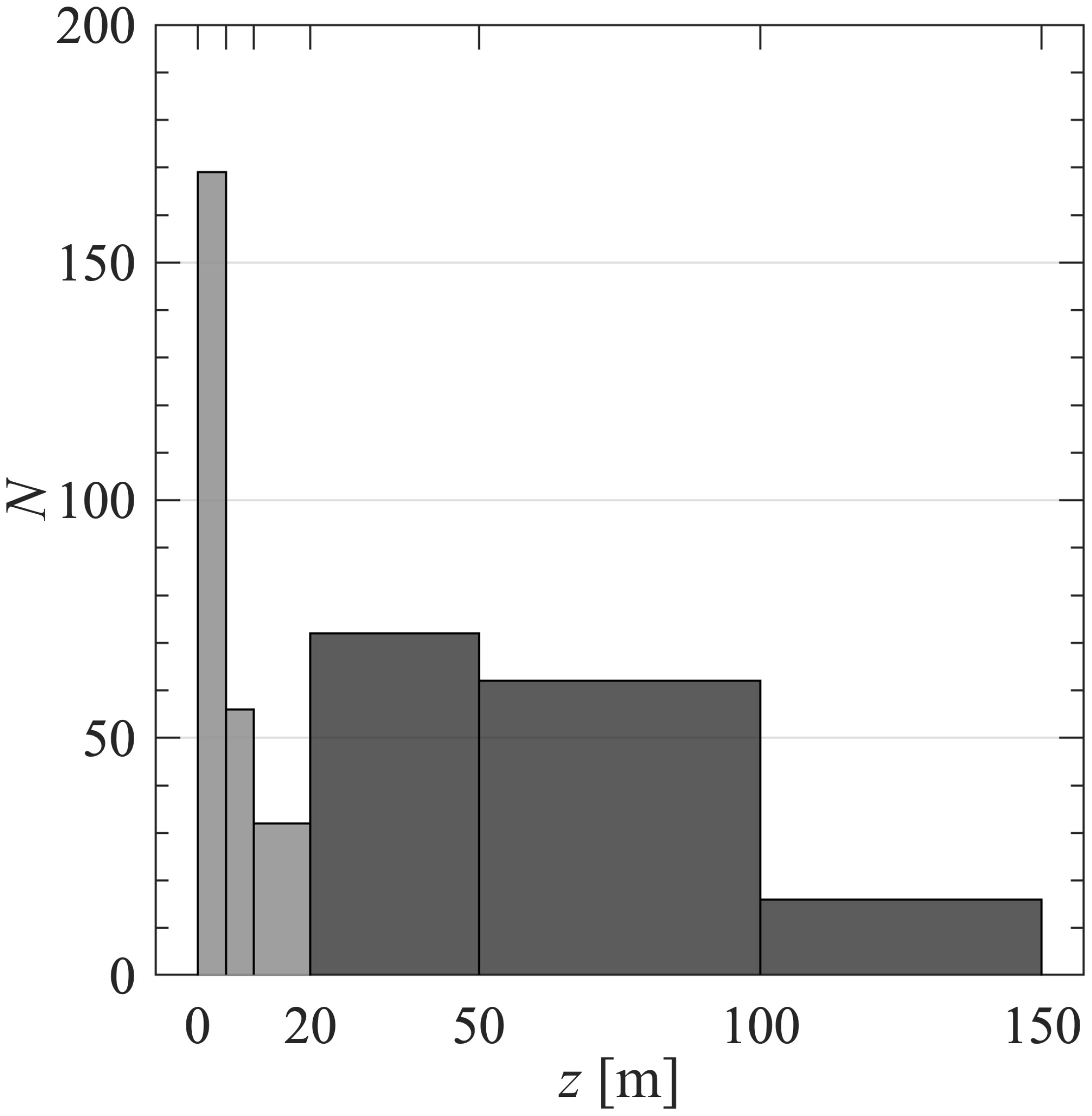
Figure 2 Histogram of sample depths z used in algorithm development dataset. Light grey denotes surface samples (z ≤ 20 m) while dark grey denotes subsurface (z > 20 m).

2.5 Algorithm development

In Koestner et al. (2022), we examined several algorithm formulations and here we focus on only the best performing versions. One of the POC algorithms that we investigate is referred to as Model A which is a univariate model with b_bp acting as a sole estimator of POC. The general form of Model A is derived from a robust ordinary least squares regression applied to POC vs. b_bp data using a power function with log₁₀-transformed b_bp and POC.

Another investigated POC algorithm is referred to as Model B which is a multivariable model. The form of Model B is an additive multiple linear regression equation with log₁₀-transformed data and an interaction term: ${\text{log}}_{10}{\text{POC}= \mathit{\text{k}}}_{\mathit{1}}{\mathit{\text{ + k}}}_{\mathit{2}}{\text{log}}_{10}{\mathit{\text{b}}}_{\mathit{\text{bp}}}{\mathit{\text{ + k}}}_{\mathit{3}}{\text{log}}_{10}\varsigma {\mathit{\text{ + k}}}_{\mathit{4}}{\text{log}}_{10}\varsigma {\times \text{log}}_{10}{\mathit{\text{b}}}_{\mathit{\text{bp}}}$, where ς = Chla/b_bp is a composition proxy and k’s are model coefficients. In this model, the second term (i.e., ${\mathit{\text{k}}}_{\mathit{2}}{\mathit{\text{b}}}_{\mathit{\text{bp}}}$) can be assumed to serve primarily as a measure of total particle concentration. The third and fourth terms relate to additional adjustments concerning bulk particulate composition based on the measurement of ς. In Koestner et al. (2022) this version of Model B was found to perform best when tested with an independent dataset. Note that all algorithm coefficients and independent variables are wavelength-dependent. Best-fit coefficients for Models A and B were computed using MATLAB’s “regress” function with a robust fitting bisquare weighting function (tuning constant = 4.685).

A bias correction function was included to improve both Model A and Model B estimations for low POC as both models tended to systematically overestimate POC at low values. Two formulations of the bias correction function were determined only for cases in which estimated POC was less than 45 mg m^-3. These determinations were made using a Model-II linear regression of observed (measured) vs. algorithm-derived (estimated) POC with and without log₁₀-transformation for power and linear versions. The bias correction function is POC = f(POC^*), where superscript * indicates initial algorithm estimation. This correction was only applied if POC^* was less than a certain threshold (ε_min) to avoid overestimation for POC greater than about 35 mg m^-3.

Prediction bounds for new algorithm estimations were computed using the coefficient covariance matrix (S) and mean-square error (MSE) determined from the regression analysis. The prediction bounds were of the form y ± e, where y is the best-fit model estimate of POC and e is the prediction uncertainty for a specific new estimation determined as $e=t\sqrt{MSE+xS{x}^T}$. In this equation, t depends on confidence level and can be calculated based on Student’s t cumulative distribution function, x is a row vector of the algorithm inputs including a value of 1 in the first element (e.g., x = [1 b_bp] for Model A), and superscript T denotes transpose operation.

The entire dataset was used for deriving model coefficients, rather than randomly splitting the dataset into development and validation datasets as was done in Koestner et al. (2022). This choice was based on the primary goal of optimizing the estimates of model coefficients through the inclusion of all available data. Algorithms were developed and evaluated using either surface samples (z ≤ 20 m) or the full dataset consisting of samples collected from all depths down to 150 m. Evaluation of algorithms used various statistical metrics to quantify and visualize uncertainty. Assessment metrics included root-mean-square deviation (RMSD), median absolute percent difference (MdAPD), median symmetric accuracy (MdSA), mean bias (MnB), and median ratio (MdR) as defined in Table 2. Coefficients of the Model-II linear regression of algorithm-derived (estimated) vs. observed (measured) POC are considered as an additional measure of algorithm performance and residual plots are also presented for additional examination of performance. A bootstrap resampling approach was also implemented in validation analysis to examine algorithm performance on 1,000 random subsets of the dataset. We utilized a subset size of 135 which was approximately one third of the full dataset and half of the surface dataset. This bootstrap procedure allows for replacement of each sample when randomly drawing a new sample to approximate 1,000 new sample populations or subsets. For each subset, statistical metrics were computed for evaluation of the variability as a function of the number of data subsets. We note that percentiles of most statistical metrics converged between 100 and 1,000 subsets.

Table 2

Table 2 Model-assessment variables.

2.6 BGC-Argo float data

BGC-Argo floats were deployed during the AMT-24 research cruise which surveyed an Atlantic Meridional Transect in the period September 24 – November 1, 2014. This cruise also involved a dedicated effort to evaluate uncertainties in POC throughout the water column down to 500 m (Sandoval et al., 2022). Data from six floats are available with vertical profiles of b_bp(700) and Chla (derived from fluorescence measurements) and five of the six floats were programmed to cycle rapidly (approximately daily) after deployment. In total, 53 profiles are available with coincident b_bp(700) and Chla that passed quality control efforts and were within the time-window of cruise operations. This results in a total of 19446 individual depth-resolved measurements available for analysis.

Float data were downloaded on September 2, 2023 from the British Oceanographic Data Centre, with the exception of one float (WMO ID 6901437) which was downloaded from the Coriolis data centre. Only adjusted Chla data which had quality control flags of 1, 2, 5, or 8 were used. The so-called “raw” b_bp(700) measurements were used, also with the same quality control flags. All data were processed to remove large particle spikes for each profile according to the methodological approach outlined in Briggs et al. (2020). As such, the resulting b_bp(700) and Chla refer to the signal from only “small” particles. A background level of b_bp(700) and Chla was determined as the 5^th percentile of values at 850–900 m from each float. This background is considered mainly as contributions from a pool of scattering or fluorescent material which appear nearly constant in the deep ocean in combination with uncertainties in manufacturer dark-counts (Poteau et al., 2017; Briggs et al., 2020). This background was removed from Chla (0.006 ± 0.003 mg m^-3) under the assumption that it is primarily driven by uncertainties in manufacturer dark-counts and any subsequent Chla values that were smaller than this background were set to 0 mg m^-3. The background was not removed from b_bp(700) under the assumption that it is driven primarily by particulate scattering which should be included in POC. The background for b_bp(700) is referred to as b_bp^Δ and was 2.0 ± 0.4 × 10^-4 m^-1.

POC was estimated using Model B described in the current study utilizing all surface and subsurface data and referred to as Ko23. An adjustment factor of 0.9 was used to account for differences between HydroScat sensors used in algorithm development and ECO sensors on floats (discussed further in section 4.3). For individual measurements when the composition term of Model B (ς = Chla/b_bp) was 0 mg m^-2 because Chla was assumed negligible or undetectable, the ς was fixed to the minimum value from the vertical profile. Minimum values of ς were 22 ± 7 mg m^-2. An additional approach commonly used with BGC-Argo float data was also implemented as an alternate estimate of POC and is referred to as Ce12 (Cetinić et al., 2012). This approach uses fixed scaling factors to convert b_bp(700) to POC within the surface mixed layer (37537 mg C m^-2) and below the surface mixed layer (31519 mg C m^-2). The Ce12 scaling factors were determined using ECO sensors and over 300 samples collected during the 2008 North Atlantic Bloom Experiment in spring near 61° N, 26° W. One other approach was also used which accounts for vertical variability in the conversion of b_bp(700) to POC and is referred to as Ga22 (Galí et al., 2022). In brief, this approach assumes an exponential decrease of scaling factor from below the surface mixed layer based on a reanalysis of Cetinić et al. (2012) data by Bol et al. (2018). The surface value of the scaling factor was set to 58968 mg C m^-2 based on Stramski et al. (2008) and an asymptote at depth was fixed to 12000 mg C m^-2. These values were assumed to be appropriate for the subtropical permanently stratified biomes (Galí et al., 2022). Surface mixed layer depths (MLDs) were determined as the depth corresponding to potential density differing by more than 0.03 kg/m^-3 of value at 10 dbar. Note that Ga22 estimates in the epipelagic zone are sensitive to MLD methodology and a detailed analysis of such sensitivity is provided in Galí et al. (2022).

All float data were acquired within the subtropical permanently stratified biome (STPS), however additional classification is performed here in accordance with partitioning of data in Sandoval et al. (2022). Floats were spatially differentiated by ecological provinces within the Atlantic Ocean (Longhurst, 2007). The relevant provinces are North Atlantic Subtropical Gyre (NAST), North Atlantic Tropical Gyre (NATL), South Atlantic Gyre (SATL), and South Subtroptical Convergence (SSTC). Further, the water column was partitioned into epipelagic (z ≤ 200 m) and mesopelagic (200 < z < 500 m) zones, again to correspond with depths evaluated in Sandoval et al. (2022).

3 Results

3.1 POC algorithms

Best fit model coefficients for univariate Model A and multivariable Model B are shown in Table 3 for b_bp at five wavelengths (i.e., 470, 532, 550, 660, and 700 nm) using only surface samples and separately for the full dataset consisting of samples collected from all depths down to 150 m. Figure 3 presents scatter plots describing Model A and Model B using three example wavelengths: 470, 550, and 700 nm. In Figures 3A, B, E, F, data for b_bp(470) and b_bp(700) are shown for the full dataset of surface and subsurface samples as these wavelengths are typically used with sensors on BGC-Argo floats and other autonomous platforms providing vertically-resolved water column observations. In Figures 3C, D, data for b_bp(550) are shown for only surface samples as 550 nm corresponds to an approximate wavelength commonly used with satellite measurement systems providing ocean color surface observations. Model A reasonably approximates the general trend of increasing POC with increasing b_bp, however there is a large scatter around the regression line (Figure 3). This scatter can generally be separated by particulate composition parameter, e.g., most datapoints with the darkest blue colors representing relatively low $\varsigma$ are typically below the regression line while lighter colors are often above the regression line. This can also be seen for the two highlighted cases in each panel referring to samples with similar POC around 100 mg m^-3, however one referring to a sample with low ς and another with high ς. There also appear no clear trends regarding region of sampling except generally larger deviations for samples from the NP ICE biome, which also tend to contain the largest contrast in terms of particle composition parameters (Figure 1B). It is worth noting that for the same dataset there is a wider range of b_bp for 700 nm compared with 470 nm (Figures 3E vs. 3A) which may provide advantages in terms of algorithm reliability in optically-clear waters. For example, when b_bp(470) = 0.0008 m^-1 there are samples with POC ranging from 10 to 70 mg m^-3 whereas b_bp(700) = 0.0008 m^-1 corresponds to a smaller range of POC of about 30–70 mg m^-3. Model A coefficients decrease with increasing wavelength, with coefficients derived at 700 nm being about 10% lower than coefficients derived with 470 or 532 nm because of increasing backscattering with decreasing wavelength (Table 3). We also can see from Table 3 and Figure 3C that Model A determined with only surface data has notably larger coefficients indicating that for all wavelengths there is on average more POC per unit b_bp in samples from the surface compared with samples from all surface and subsurface depths.

Table 3

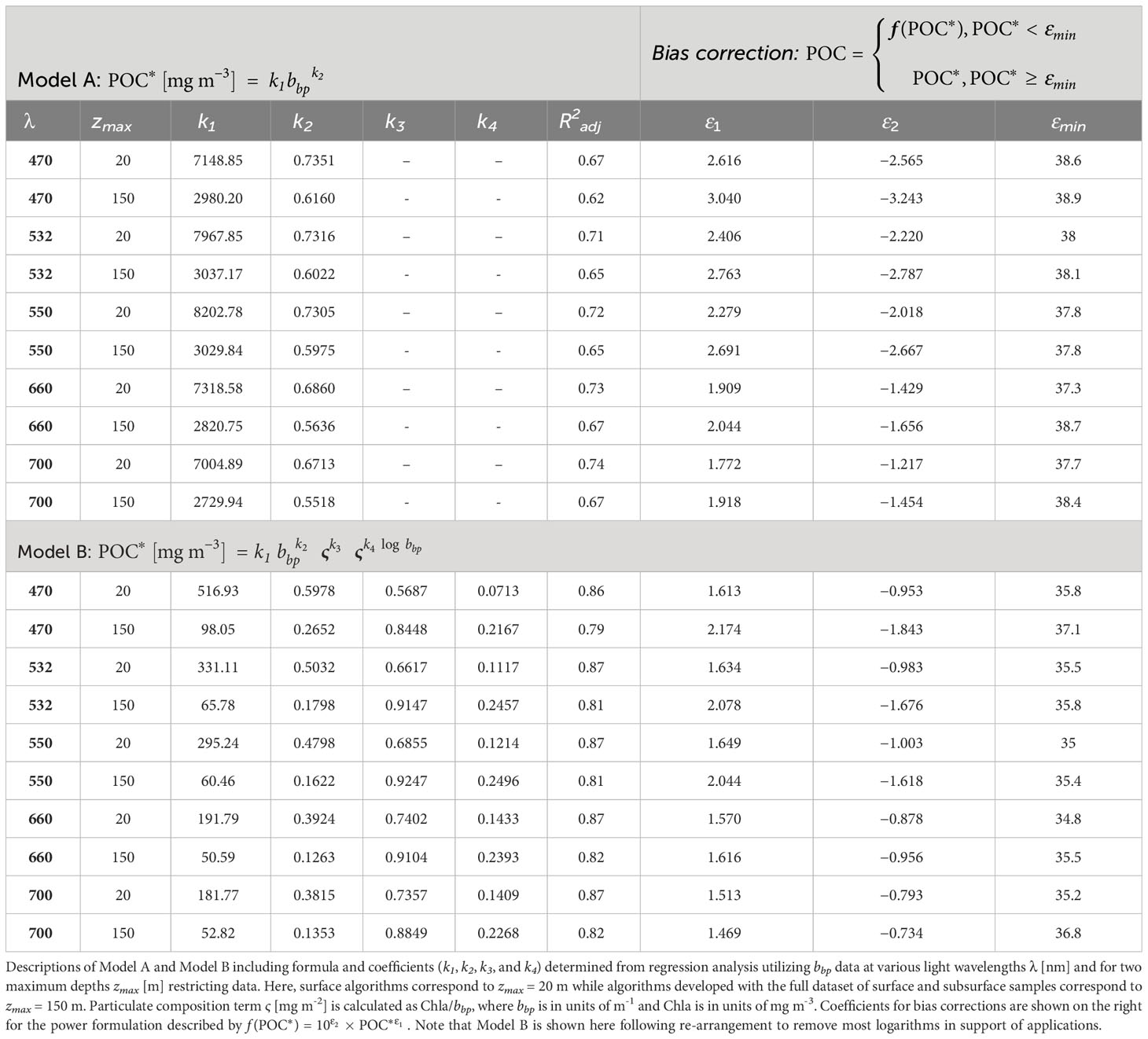
Table 3 Algorithms for estimating POC.

Figure 3

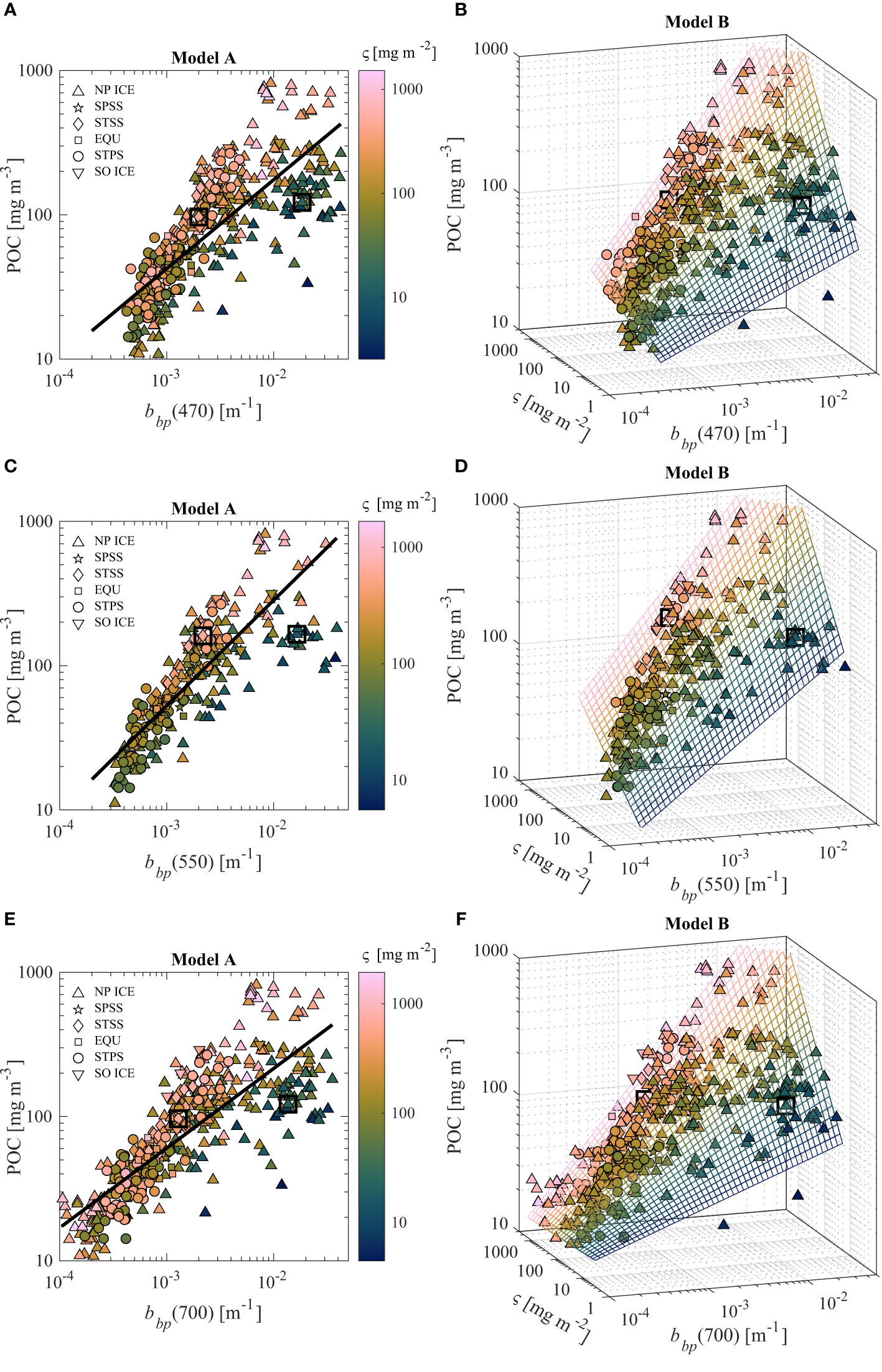
Figure 3 Univariate (A, C, E) and multivariable (B, D, F) algorithms to estimate POC utilizing light wavelength of 470, 550, and 700 nm. Algorithms in (C, D) utilize only surface samples for formulation (N = 257) while other algorithms utilize the entire dataset (N = 407). Data are color coded by the value of particle composition parameter ς = Chla/b_bp. Two data points which contrast in terms of ς but contain similar levels of POC are marked with a square for discussion purposes.

Figure 3 also depicts 3-dimensional scatter plots with mesh-grids representing Model B results. The inclusion of an additional independent variable related to particle composition (i.e., ς) results in better representation of the POC data (e.g., R²_adj = 0.79–0.87 for Model B and R²_adj = 0.65–0.74 for Model A; Table 3). The mesh-grids detail steeper slopes of POC vs. b_bp for high ς compared with low ς (Figures 3B, D, E). In other words, for samples likely to have relatively high proportions of phytoplankton (high ς), larger values of POC are found for the same amount of particulate backscattering as compared with samples with a lower abundance of phytoplankton. This matches our expectation; non-phytoplankton particles can efficiently backscatter light, especially inorganic material that does not contribute to POC, and, conversely, phytoplankton particles generally contribute significantly to POC while having lower relative contribution to light backscattering. The ability of Model B to account for the variability in particle composition when estimating POC based on particulate backscattering and chlorophyll-a measurements can provide strong advantages for samples which vary in terms of particle composition, as is often the case in natural waters. Similarly, as seen with Model A, the Model B coefficients generally decrease with increasing wavelength and are notably larger when determined with surface samples compared to all samples (Table 3). Interestingly, k₃ for Model B, which refers to the exponent of the composition parameter, varies very little (less than 2%) for Model B determined using all data and light wavelengths of 532, 550, 660, and 700 nm (Table 3). This suggests that the weighting of this composition term in Model B can be quite consistent regardless of wavelength while all other coefficients account for variability associated with wavelength.

A positive bias for Model A and Model B can be observed in Figure 3, particularly when POC is lower than about 40 mg m^-3. Koestner et al. (2022) proposed a low-POC bias correction for Model B based on a linear function and we extend this approach to Model A along with two different formulations of the bias correction function. Figure 4 depicts scatter plots of uncorrected algorithm estimates of POC vs. measured POC with two functional fits of the data for bias correction (i.e., linear and power models). In Figure 4, we present results based on the algorithms determined with b_bp(550) and the full dataset to demonstrate trends in bias and we extrapolate bias correction functions to measured POC = 3 mg m^-3 which can be considered a lower limit of detection for conventional POC methodology (Sandoval et al., 2022). Prior to bias-correction, Model B outperforms Model A in terms of accuracy (i.e., RMSD and MdSA) and bias (i.e., MnB and MdR) for POC < 60 mg m^-3 (Figure 4). However, both models exhibit a positive bias in the range of POC < 60 mg m^-3 (e.g., in this range MdR is 1.22 and 1.12 for Model A and Model B, respectively). After applying a bias correction, RMSD is quite consistent for both Model A and Model B, however Model A does have reduced MdSA (29% before and around 25% after correction in the range of POC < 60 mg m^-3). Of most importance, the positive aggregate bias in terms of MdR for POC < 60 mg m^-3 is reduced to the ideal value of around 1 after bias correction (Figure 4). Although the differences between the application of linear or power functions for bias correction are minimal, we believe that the power function will be more reliable given that the linear bias correction can result in negative POC after correction if estimated POC is less than the y-intercept and the power function is generally more conservative for POC less than about 15 mg m^-3 (Figure 4). Thus, we recommend the power function form for bias correction and accordingly provide model coefficients for this case in Table 3. We note that there are similar trends in terms of bias for other wavelengths except that there are generally smaller bias corrections for longer wavelengths (e.g., Table 3 and Figure 3).

Figure 4

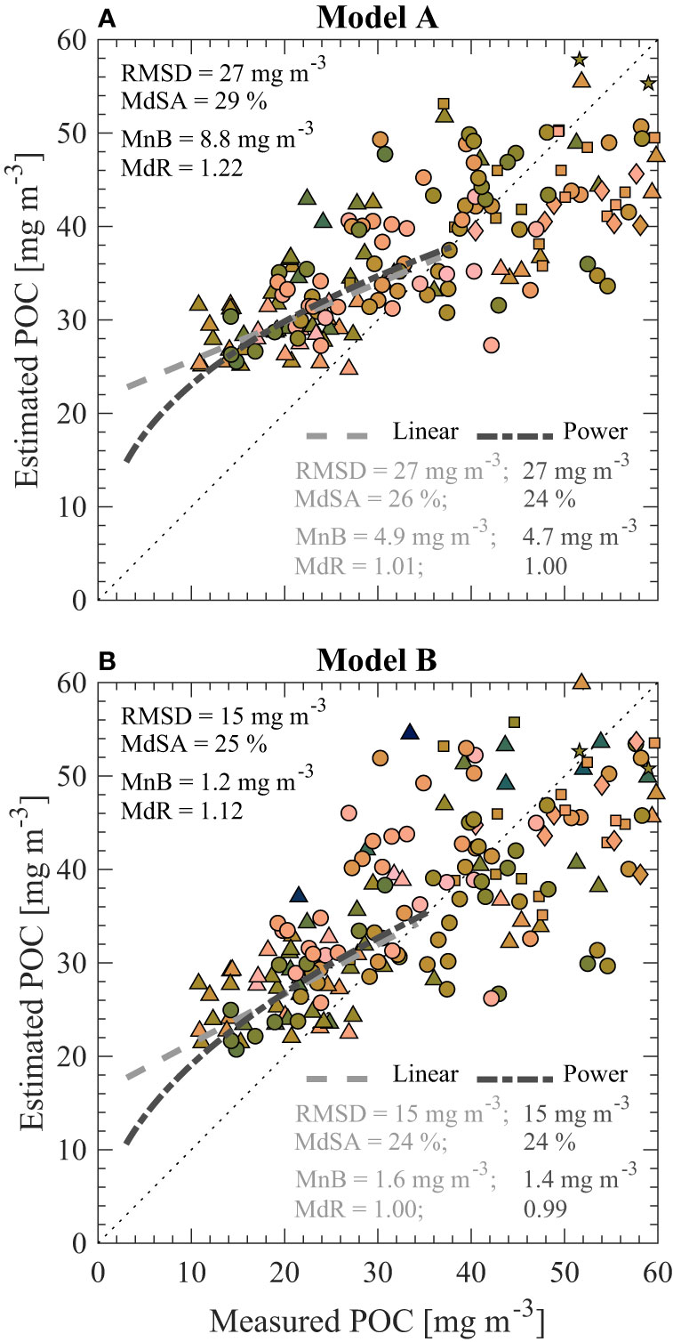
Figure 4 Example of algorithm-derived (estimated) vs. observed (measured) POC before any bias-correction for (A) Model A and (B) Model B developed using b_bp(550) and the full dataset (N = 407). Statistical metrics are displayed and computed for measured POC< 60 mg m^-3 (N = 189). Metrics displayed in top left refer to estimated POC before any bias-correction while numbers in bottom right denote metrics derived after applying the linear (light grey) and power (dark grey) functions for bias-correction. Note that bias correction functions are extrapolated to measured POC = 3 mg m^-3, a reasonable lower limit of detection for conventional POC methodology (Sandoval et al., 2022).

3.2 Validation

In the following figures, we present results from validation exercises based on comparison of measured POC with bias-corrected estimates from Model A and Model B. In Figures 5–7, we describe statistical assessment of the six examples shown in Figure 3 through comparison of estimated and measured POC. Next, we present a summary of the bootstrapping validation analysis for all model formulations (Figure 8). Finally, we take advantage of our relatively large dataset to assess other optical approaches for estimating POC found in the literature (Figure 9).

Figure 5

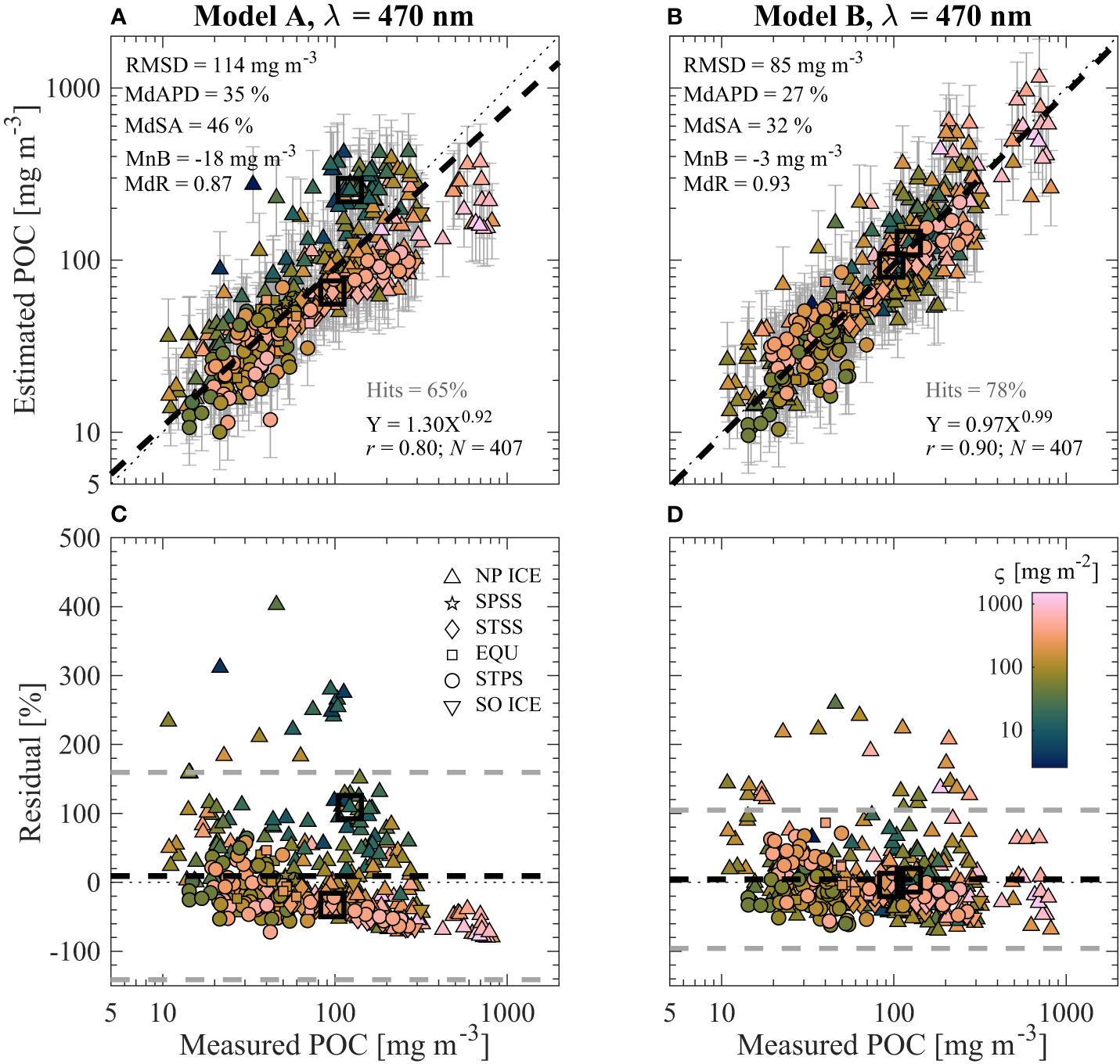
Figure 5 Validation of (A, C) Model A and (B, D) Model B through comparison of algorithm-derived (estimated) and observed (measured) POC for bias-corrected estimates from algorithms utilizing b_bp(470) and the full dataset shown in Figures 3A, B. Data are color coded by the particle composition parameter ς described by color bar in (D). Two data points are marked with a square to illustrate effectiveness of Model B with contrasting particle composition. (A, B) Algorithm-derived (estimated) vs. observed (measured) POC. Statistical metrics described in Table 2 and derived from this comparison are shown. Model-II linear regressions of log₁₀-transformed data are displayed with a dashed line and equation is shown, where X and Y refer to measured and estimated POC, respectively. A 1:1 dotted line is plotted for reference. Hits describe the percentage of datapoints whose prediction error bars (two-tailed, α = 0.125) contain the measured value. (C, D) Residual plots from data in panel above. Percent residuals are defined as 100% × (Estimated POC – Measured POC)/Measured POC. Black dashed line represents mean residual value while grey dashed lines represent approximate 95% confidence limits of residuals (i.e., mean ± 1.96 standard deviations).

Figure 6

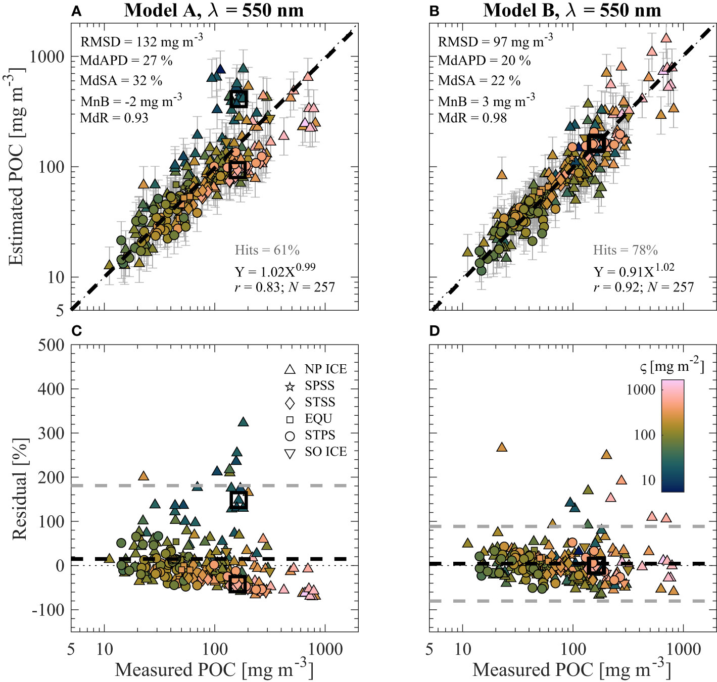
Figure 6 Similar to Figure 5 but utilizing algorithms for b_bp(550) developed with only surface data shown in Figures 3C, D.

Figure 7

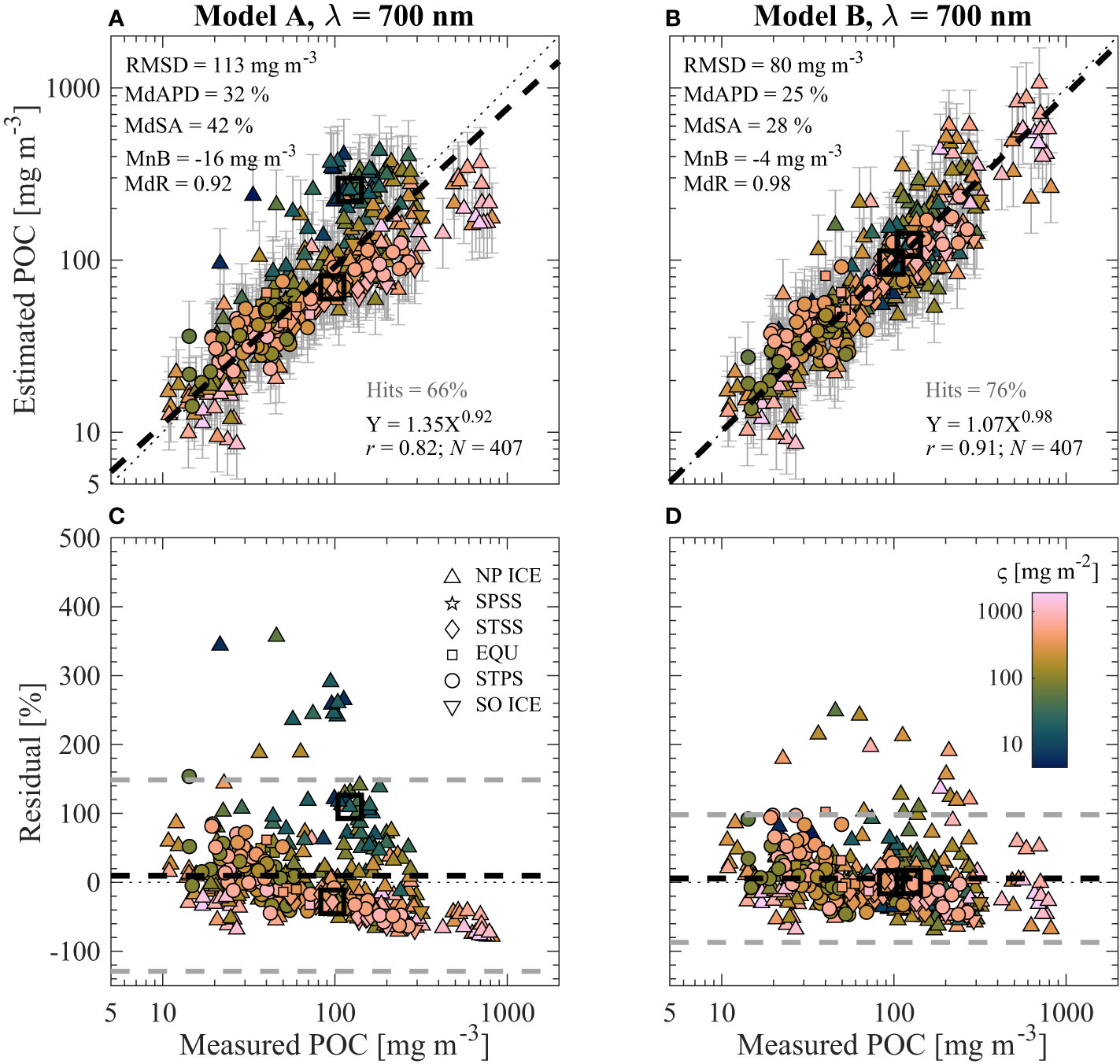
Figure 7 Similar to Figure 5 but utilizing algorithms for b_bp(700) developed with the full dataset shown in Figures 3E, F.

Figure 8

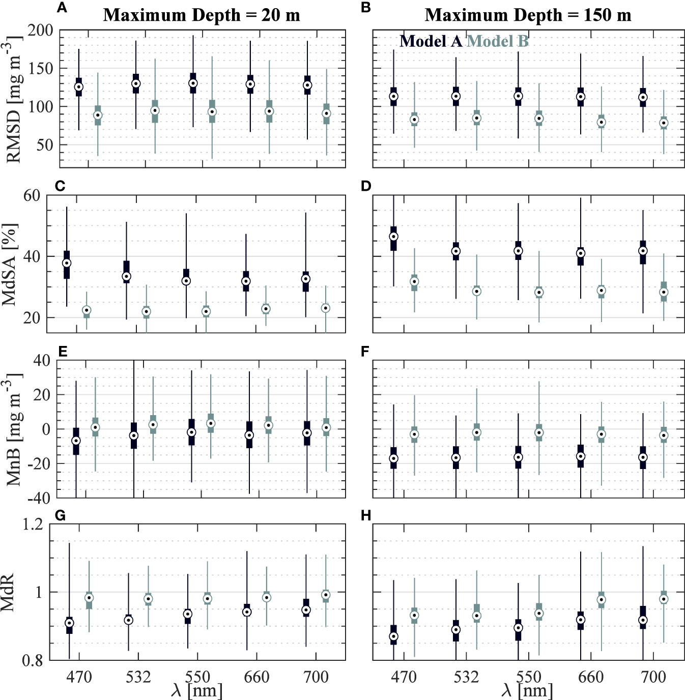
Figure 8 Nonparametric box plots summarizing performance of all algorithms using a bootstrap sampling approach for validation statistics. In each box plot, whiskers represent the entire range while the box contains the semi-interquartile range and circles denote median. Box plots are derived based on 1,000 repetitions of random sampling of 135 datapoints with replacement allowed. (A, C, E, G) Statistics for the algorithms developed with only surface data. (B, D, F, H) Statistics for the algorithms developed with full dataset.

Figure 9

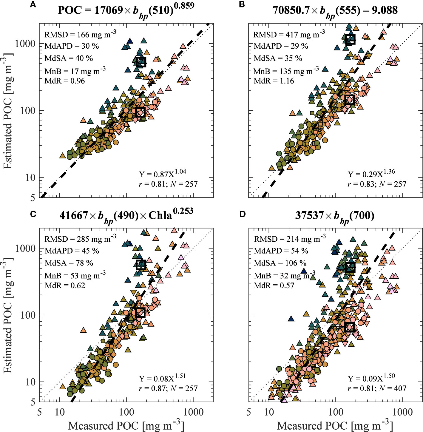
Figure 9 Validation results similar to Figures 5A, B comparing algorithm-derived (estimated) and observed (measured) POC using four previously published approaches relating b_bp to POC: (A) Stramski et al. (1999) using data from Antarctic Polar Front Zone, (B) Stramski et al. (2008) using data from the Pacific and Atlantic Oceans and subtraction of backscattering by pure water according to Buiteveld et al. (1994) with additional correction for salinity of pure seawater, (C) Loisel et al. (2002), and (D) Cetinić et al. (2012) using only the slope of POC vs. b_bp(700) for downcast data within the oceanic mixed layer. Equations are shown above each panel and (D) includes the full dataset from the present study while the other relationships in (A–C) are examined only with surface data from the present study.

In Figures 5–7, multivariable Model B outperforms univariate Model A in terms of all statistical metrics evaluated over the entire dynamic range of the investigated dataset. This is the case for algorithms developed with the full dataset as well as only surface data (e.g., Figure 6). Although Model A performs reasonably well for POC less than about 100 mg m^-3, there is a clear compositional dependence on performance where more algal-dominated (i.e., high ς value) samples tend to be underestimated and nonalgal dominated (i.e., low ς value) samples are overestimated (e.g., Figure 5C). This issue is not as apparent for Model B where there are no clear trends of over- and underestimation in terms of particle composition (e.g., Figure 5D). The major improvements in Model B can also be observed when examining the cluster of samples with low or high ς values from the Arctic which have Model A estimated POC of around 200–300 mg m^-3 (e.g., Figure 5A). Whereas Model A greatly overestimates the datapoints with low composition values and underestimates the datapoints with high composition values, Model B is able to correctly adjust its estimates of POC much closer along the 1:1 line due to the inclusion of composition-specific independent variable ς (e.g., Figure 5B). Furthermore, the two contrasting samples from completely different oceanic biomes (i.e., Atlantic Ocean STSS and Arctic Ocean NP ICE near Alaska) shown in Figures 5–7 are correctly estimated by Model B (less than about 3% differences from measured POC) while they are incorrectly estimated by Model A (about 30% to over 100% differences from measured POC).

In the current study, our primary emphasis is on optimizing the determination of algorithm coefficients by using a relatively large dataset containing available measurements from diverse oceanic conditions. Thus, we did not split the available dataset into independent subsets of data for algorithm development and validation purposes, as was done in Koestner et al. (2022). In this study, we employed a bootstrap resampling approach to investigate algorithm performance on random subsets of the entire algorithm development dataset. Figure 8 presents a summary of this analysis focusing on the variability in four statistical metrics derived from the 1,000 subsets and using all algorithm formulations in Table 3. Here, we focus on RMSD and MdSA for quantifying magnitude of the random component of uncertainty while MnB and MdR are used to describe bias. Again, Model B has lower uncertainty and less bias for all formulations when compared with Model A for the overwhelming majority of random subsets (Figure 8). In terms of uncertainty magnitude, Model B typically has MdSA of 20–35% and RMSD of about 70–110 mg m^-3 depending on wavelength and dataset utilized. For example, there are somewhat larger MdSA values (rarely below 25%) for Model B developed and tested with the full dataset while median values of MdSA are around 22% when considering only surface data. Differences associated with wavelength utilized are minor, however when considering Model B formulated with the full dataset, there may be some small advantages in terms of MdR when utilizing λ = 660 or 700 nm (Figure 8). Spectral differences are even smaller when considering surface-only algorithms.

Figure 9 depicts comparisons of measured POC with algorithm-derived (estimated) POC using four other algorithms found in the literature. Two algorithms presented here (i.e., Stramski et al., 1999 and Stramski et al., 2008) were developed using a small portion of the data included in the present study, however, they are tested on the entire dataset of surface samples consolidated for the current study. The Loisel et al. (2002) algorithm combines two approaches: one to estimate the scattering coefficient based on the backscattering coefficient and Chla (Twardowski et al., 2001) and another to relate the scattering coefficient to POC (Claustre et al., 1999). These three algorithms are evaluated for only surface data as they have been proposed as potential candidate algorithms for estimating POC based on remote-sensing reflectance observations (Loisel et al., 2002; Stramski et al., 2008; Evers-King et al., 2017). The fourth algorithm is from Cetinić et al. (2012) and has been commonly used to estimate POC with in situ measurements from platforms such as BGC-Argo; thus, we present evaluation based on the full dataset with sample depths down to 150 m. Although all algorithm estimates have some regions of reasonable agreement with POC measured using standard methodology (typically around 100 mg m^-3), there are large deviations resulting in relatively high values of some aggregate statistical metrics (Figure 9). These relatively simple approaches may produce reasonably good estimations for water types similar to those used in the algorithm development, however large uncertainties are observed when considering the wide range of contrasting optical and particle properties in our dataset. The advantage of Model B to adapt to a variety of environments can offer useful advantages when examining POC estimates from optical measurements collected across diverse water bodies including large ocean scales.

Finally, we consider comparisons of the 700 nm version of Model B from our previous study (Ko22; Koestner et al., 2022) with the current formulation determined with the larger dataset of surface and subsurface samples. Coefficients from the current study are somewhat different (e.g., k₁ and k₂ are smaller while k₃ and k₄ are larger compared to Ko22). In terms of aggregate statistics based on analysis with the full dataset, there are no appreciable differences between the formulation from Ko22 and the current version (e.g., RMSD = 68 mg m^-3, MdAPD = 25%, MdSA = 29%, MnB = −6 mg m^-3, and MdR = 1.01 for Ko22; compare with current values in Figure 6B). Generally, the largest differences between the two models relate to about a 10% underestimation of POC for highest composition values and about a 10% overestimation for lowest composition values in the Ko22 model compared with current Model B estimations. There are some additional differences when considering POC < 35 mg m^-3 which relate more directly to the use of bias correction recalling that Ko22 utilized a linear bias correction function. We expect some of the above-mentioned differences to relate to refinements in Chla data from ANTXXVI/4 cruise as well as the addition of some “new” data and application of several inclusion/exclusion criteria in the compilation of the dataset for the current study. Additionally, current Model B coefficients all have smaller uncertainty (in terms of 95% confidence intervals) and are more statistically significant (in terms of p-value) compared with coefficients in Ko22. For example, current coefficients have confidence intervals which are between 30% and 180% of their best-fit coefficient value and p-values less than 10^–16, apart from k₂ with a p-value of 0.03. For Ko22 coefficients, confidence intervals were nearly twice as large (60–280% of their best-fit coefficient value) and p-values were less than 10^–5 with the exception of k₂ with a p-value of 0.06. As a result, we recommend use of the current formulation of Model B.

4 Discussion

4.1 Depth dependencies

As seen in Table 3, there are noticeable differences in algorithm coefficients derived using only surface data compared with the full dataset. We also found that algorithms developed and tested with only surface data generally had improvements in the model performance (Figure 8). It is desirable to apply a single approach when making assessments of the vertical structure of POC with in situ measurements; therefore, we examine how well Model A and Model B perform with surface data when developed with the full dataset in Figure 10. Overall, these algorithms perform well when examining only surface data. For example, Model B estimations typically differ by less than about 25% from measured POC in terms of MdAPD and MdSA (Figures 10B, D). Surprisingly, when evaluating the surface data, RMSD is lower for the algorithms developed with the full dataset compared with versions developed with only surface data (e.g., Figures 10A, B vs. 6A, B). We believe this counterintuitive reduction in RMSD illustrates that RMSD is not always a reliable measure of performance as it is not a proportional or symmetric metric because larger magnitude errors are more heavily weighted. Unlike the algorithm versions developed with only surface data, the Model B algorithms presented in Figure 10 display systematic underestimation as seen with MnB of about –20 mg m^-3 and MdR around 0.82–0.86. Moreover, this underestimation is quite small for lower POC but worsening with increasing POC as illustrated with the linear regression line of estimated vs. measured POC (Figures 10B, D). Importantly, we recall that the majority of the surface samples are from depths less than 5 m (Figure 2), and these biases are likely minor when considering large portions of the water column including the epipelagic layer or deeper. Nonetheless, we generally recommend using the model coefficients derived with only surface samples when the investigation is focused on surface waters, for example with satellite or other above-water observation systems. When the investigation is focused on vertically-resolved measurements within the water column (for example with BGC-Argo floats or gliders), we recommend using model coefficients derived with the full dataset of surface and subsurface samples.

Figure 10

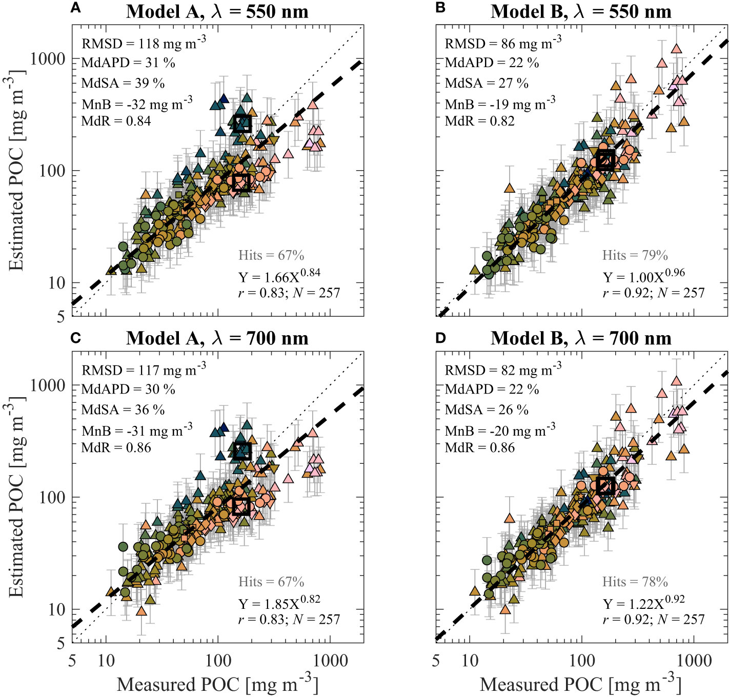
Figure 10 Validation results similar to Figures 5A, B comparing algorithm-derived (estimated) and observed (measured) POC for only surface data using algorithms developed with the full dataset. Descriptions regarding algorithm used (i.e., model and wavelength of b_bp) are above each panel. (A) Model A, λ = 550 nm. (B) Model B, λ = 550 nm. (C) Model A, λ = 700 nm. (D) Model B, λ = 700 nm.

4.2 Biomes

Our algorithm development dataset is composed of samples collected in 6 oceanic biomes, however samples are not evenly distributed among these biomes and across all seasons (Figure 1B and Table 1). For example, only 4 samples are in the subpolar seasonally stratified biome (3 of which are from the Southern Ocean), and only 6 samples are in the Southern Ocean marginal sea ice biome. A large portion of the data is from the North Pacific marginal sea ice biome which importantly incorporates samples which are not organic-dominated and not algal-dominated into the dataset (Figure 1B). This contributed to a compositionally diverse dataset for algorithm development, however, it may produce some bias when examining other samples in other biomes. Here, we examine the uncertainties in POC estimations within each biome separately using Model A and Model B from the current study, as well as four algorithms from the literature which have already been shown in Figure 9.

Figure 11 depicts the statistical variability in percent difference of algorithm estimates from measured POC. Model B outperforms nearly all algorithms for the four main biomes sampled, with the exception of the subtropical seasonally and permanently stratified biomes (STSS and STPS) where Stramski et al. (2008) and Stramski et al. (1999) algorithms respectively display minor improvements (Figure 11). Of note, Model B performs well in the NP ICE, EQU, and STPS biomes, where median percent differences are less than 5%. Based on this dataset, it appears that Model A and Model B have the largest biases in the STSS and SO ICE biomes in that over 75% of the samples have POC underestimations by more than about 10%. This difference is largest in SO ICE with a median underestimation of 35% for Model B (noting that only 6 samples are available for this analysis). In STSS, median underestimation for Model B is only 14%. The Ce12 algorithm consistently produces large underestimations (>25% for majority of samples and >50% for most biomes). We suspect this result may be associated with differences in POC methodology (IOCCG Protocol Series, 2021; Sandoval et al., 2022) and backscattering instrumentation (e.g., Erickson et al., 2022), and the fact that the Ce12 dataset was collected in the North Atlantic subpolar seasonally stratified (SPSS) biome during spring. Although Model B performs well in the SPSS biome (Figure 11), we acknowledge that only 4 samples are available for the current study. Further investigation and inclusion of more data, especially from the SPSS and SO ICE biomes and all biomes during winter months, is highly desirable to support potential refinements of algorithms and more comprehensive validation.

Figure 11

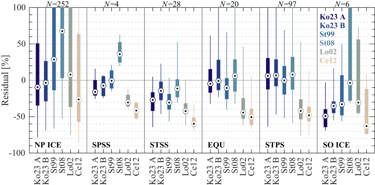
Figure 11 Nonparametric box plots summarizing performance of various POC algorithms for available data within each oceanic biome as indicated. In each box plot, whiskers represent the entire range while the box contains the semi-interquartile range and circles denote median. All surface and subsurface data are used to derive percent residuals, defined as 100% x (Estimated POC – Measured POC)/Measured POC. Ko23 A and Ko23 B refer to Model A and Model B from current study utilizing λ = 700 nm and the entire dataset. The four additional algorithms are described in Figure 9 noting that St99 refers to Stramski et al. (1999), St08 refers to Stramski et al. (2008), Lo02 refers to Loisel et al. (2002), and Ce12 refers to Cetinić et al. (2012).

4.3 Uncertainties and implications to applications

The algorithm development dataset mainly utilized Chla derived from HPLC analysis and spectral b_bp derived at 6 to 11 wavelengths with HydroScat-6 instruments (HS-6). This was to avoid additional uncertainties and establish reliable algorithms describing the relationships between spectral b_bp, particle composition approximated with ς = Chla/b_bp, and POC. In most applications, however, Chla will be retrieved from either in situ fluorometric measurements or ocean color remote sensing observations and b_bp will be retrieved from in situ scattering measurements (most likely with different instruments) or satellite observations including lidar or passive ocean color remote sensing. Here, we discuss some of the potential uncertainties associated with different sources of algorithm inputs and how they may impact applications of Model B to estimate POC.

In situ fluorometric estimates of Chla have been shown to contain systematic biases when compared with HPLC-derived Chla and significant efforts have been made to reduce these uncertainties (e.g., Xing et al., 2012; Roesler et al., 2017; Xing et al., 2017). With regards to processing of in situ fluorometric data from ECO-series fluorometers on BGC-Argo floats, a community-established bias factor of 2 is often applied, however it has been shown to be as high as 4–6 in various oceanographic regions (Roesler et al., 2017). Routinely implemented algorithms which estimate Chla from current satellite ocean color observations achieve median absolute errors of up to 60–70% based on analysis of over 2000 satellite and in situ matchups spanning the global oceans (O’Reilly and Werdell, 2019). For the purposes of illustrating propagation of uncertainty in Chla to Model B estimations of POC, we assume a 65% error for Chla. For this case, the resulting uncertainty in POC estimated from Model B is typically much less than 65%. For example using realistic values for productive ocean surface water of b_bp(700) = 0.001 m^-1 and Chla = 0.5 mg m^-3, the Model B estimate of POC is about 74 mg m^-3 with a prediction interval of 46–118 mg m^-3 (approximately 75% confidence). Assuming that Chla is 65% larger, POC estimation only increases by about 11% to 82 mg m^-3 which is well within the prediction interval. This suggests relatively weak sensitivity of algorithm estimates of POC to uncertainty in Chla.

Regarding b_bp uncertainty, a community standard similar to HPLC for Chla does not yet exist. Estimating b_bp with single-angle backscattering measurements is expected to result in errors typically less than 10% (Boss and Pegau, 2001; Sullivan et al., 2013). Analysis of over 16,000 BGC-Argo float profiles found approximately 30–50% differences when comparing median values of b_bp(700) between 900–950 m from 200 floats which were equipped with one of three sensor types (Poteau et al., 2017). For satellite-based retrievals of b_bp from lidar or passive ocean color observations, 20–50% uncertainty is reasonable based on limited comparisons of satellite b_bp retrievals and in situ measurements (Loisel et al., 2018; Bisson et al., 2021; McKinna et al., 2021). Here we also acknowledge that uncertainties in b_bp retrievals from lidar or passive ocean color observations are dependent on wavelength as well as statistical approaches utilized in defining uncertainty and accepted “true” in situ b_bp values. Nevertheless, if we assume that b_bp(700) is 30% higher, POC estimated from Model B using the above example is about 85 mg m^-3, an increase of about 15%. Again, this exemplifies the robustness of Model B estimations. Finally, combining 30% and 65% overestimations for b_bp and Chla, respectively, we find that Model B estimated POC is about 95 mg m^-3, an overestimation of 27% but still within the prediction interval defined above.

We also acknowledge that differences have been observed between HS-6 and other backscattering sensors likely owing to differences in instrument calibration procedures, data processing, and instrument geometries. For example, Erickson et al. (2022) observed lower values by about 30% on average for b_bp(700) from HS-6 when compared with ECO sensors (two or three channel sensors formerly produced by WET Labs, currently Sea-Bird Scientific) which are typically deployed on BGC-Argo floats and gliders. This comparison involved intercomparison of several backscattering sensors deployed during the EXPORTS field campaign in the North Pacific Ocean. In contrast, Twardowski et al. (2007) observed good agreement in very clear South Pacific Ocean waters during the BIOSOPE cruise with HS-6 b_bp(470) about 4% lower on average than b_bp(462) from an ECO-BB3. Similarly, others found that b_bp(530) from an HS-6 was also about 3% lower than the ECO-VSF b_bp(532) in very clear waters of Crater Lake Oregon (Boss et al., 2007) and less than 2% lower for coastal shelf waters in the Mid-Atlantic Bight (Boss et al., 2004). Note that the ECO-VSF instrument is somewhat different than other ECO sensors as it measures scattering at three angles from the incident light direction at approximately 104°, 124°, and 151° whereas other ECO sensors typically measure scattering of light at one scattering angle (usually approximately 124° or 142° from incident direction). In our own, but limited, studies we have observed differences for b_bp(700) from HS-6 (close to 12% lower on average) compared to an ECO-Triplet deployed on the same optical package for 12 stations in coastal Alaska. We also observed a 1–26% (median of 10%) lower b_bp(532) from HS-6 compared with the LISST-VSF (Sequoia Scientific) based on a 40-minute time series of simultaneous measurements off the Scripps Institution of Oceanography Pier in La Jolla, California where LISST-VSF-derived b_bp(532) was about 0.0085 m^-1. Unlike other scattering instruments, the LISST-VSF measures backscattered light from 90–150° in 1° increments and therefore requires less assumptions about the shape of the angular scattering function than other single or multi-angle sensors (Koestner et al., 2018). We expect the above-mentioned differences in b_bp are mainly related to data processing steps including assumptions about angular scattering function, pure water and baseline subtraction, calibration scaling factors, and corrections for losses along path to and from the sample volume. Overall, however, the HS-6 instrument appears to yield systematically lower values of b_bp when compared with several different instruments. Therefore, when applying algorithms developed entirely with HS-6 data (such as Model A and Model B from the current study) to b_bp measurements from other backscattering sensors, a normalizing factor for b_bp can be considered. For example, applying a multiplicative factor of 0.9 to measurements with ECO-like instruments may provide a reasonable average factor accounting for these differences. However, we recommend caution if applying this factor as it will likely depend on data processing, specifics of the sensor, and particulate and optical properties of seawater. Importantly, this will not result in the reduction of POC by the same factor; rather it is often a smaller change in POC dependent on Chla and b_bp. For example, using the case described in the previous paragraphs, multiplication of b_bp by 0.9 results in POC of about 70 mg m^-3, or a reduction of approximately 5%.

There are some additional considerations when applying Model B to measurements in optically clear waters such as deep waters in the mesopelagic zone below 200 m or ultraoligotrophic surface waters often surveyed with BGC-Argo floats. Our algorithm development dataset did not include any samples deeper than 150 m (Figure 2) and mesopelagic POC values are generally expected to be near the lower limit of 10 mg m^-3 utilized in our algorithm development (e.g., Sandoval et al., 2022). For this reason, we expect the choice of bias correction function will strongly influence algorithm estimations of mesopelagic POC less than about 20 mg m^-3 (see Figure 4), as will the treatment of data in terms of background subtraction, spike removal, vertical averaging, and inclusion of POC estimates outside of the algorithm development range. Additionally, instrument sensitivity and calibration will also play a more significant role when backscattering signals become very low in the mesopelagic or very clear surface waters. Finally, reliance of the particulate composition term on Chla inherently carries some challenges when considering that mesopelagic waters usually have low ς values regardless of their nature as the composition term is likely poor at distinguishing between nonalgal type, whether it be inorganic and contributing nothing to POC (e.g., calcium carbonate or silica) or organic with no chlorophyll-a content but contributing to POC (e.g., detrital material or heterotrophic bacteria). We recommend fixing ς to some minimum value if Chla is effectively zero (i.e., below detection limit), and when vertical profiles of measurements are available, it is appropriate to use a minimum nonzero value of ς determined from the profile. Furthermore, we also recommend fixing ς to a value of 2000 mg m^-2 at a maximum because values higher than this are unlikely to be observed in the ocean (e.g., Figure 1B; Barbieux et al., 2018) and can be related to very low signal from both Chla and b_bp.

Finally, it is of the utmost importance to recognize that POC is an operationally-defined parameter, whereas b_bp is defined more precisely as the backscattering coefficient with contributions of pure water and dissolved salts removed. Operationally, POC is the “particulate” pool of organic carbon usually defined as the mass concentration of organic carbon retained on GF/F filters with a nominal 0.7 µm pore size. Typically, some amount of truly “dissolved” carbon is also included in the POC due to adsorption of dissolved organic carbon (DOC) to the GF/F filters (Moran et al., 1999; Novak et al., 2018). This adsorption effect is typically minimized by (1) filtering a sufficient volume of water so that the “particulate” signal retained on the filter overwhelms the adsorbed “dissolved” signal, and/or (2) subtracting a “wet” blank filter created with GF/F filtrate (IOCCG Protocol Series, 2021). The POC used in the current algorithm development dataset mostly did not include any subtraction of a “wet” blank, but rather filtration of large volumes of seawater which may still introduce some positive bias of POC due to DOC adsorption, likely by at most 10 to 20% (Stramski et al., 2022). Very importantly, however, the correction for DOC adsorption was purposefully not made because the measurement of POC on GF/F filters is missing some portion of carbon from colloidal particles which contributes to total POC (e.g., small bacteria and phytoplankton cells, viruses, and other small-sized detrital material). This missing portion of POC, in addition to other sources of negative bias, leads to an underestimation of total POC which is expected to largely balance the positive biasing effect due to uncorrected adsorption of truly dissolved DOC. Thus, the resultant estimate of measured POC without correction for DOC-adsorption is expected to provide a closer agreement with total POC (including all suspended particles) compared to POC measurement corrected for DOC-adsorption alone (Stramski et al., 2022). This is critical from the standpoint of relating measured POC to measured optical properties. In particular, the measured b_bp is, in principle, influenced by all particles, including a portion of small colloidal particles not included in POC collected on GF/F filters (Organelli et al., 2018; Stramski et al., 2004; Stramski and Woźniak, 2005; Zhang et al., 2020). It is therefore sensible to correlate the measured b_bp associated with all particles with the best possible estimate of total POC. This distinction is important to consider when comparing results of Model A or Model B with other estimates of POC, either from measurement results with GF/F filters from other studies or from biogeochemical modeling results (e.g., Galí et al., 2022; Wang and Fennel, 2023), as we consider our algorithms to provide optimal estimates of total POC with the currently available methodology of POC determinations on GF/F filters.

4.4 Application to BGC-Argo floats

The AMT-24 research cruise provided a unique opportunity to examine an independent dataset spanning several distinct ecological provinces within the subtropical permanently stratified (STPS) biome of the Atlantic Ocean in late 2014. Here, POC estimates from optical measurements on BGC-Argo floats are compared with POC derived from traditional discrete water sampling to depths of 500 m made during the cruise (Sandoval et al., 2022). Importantly, we note that Sandoval et al. (2022) utilized a DOC-adsorption correction for POC based on the double-filter method which reduced POC by about 10–20% due to presumed adsorption of DOC.

A summary of BGC-Argo floats and the AMT-24 cruise is shown in Figure 12A and corresponding vertical profiles of POC derived from our present Model B (hereafter referred to as Ko23) are shown in Figure 12B. We note that only float profiles within the time-window of cruise operations are examined here. Each ecological province appears to have distinct vertical POC profiles and individual float profiles are generally consistent within each ecological province; however, some differences are observed. For example, the depth associated with maximum POC for the two floats in North Atlantic Tropical Gyre (NATL) vary, while differences are seen for individual profiles within the South Subtropical Convergence (SSTC) province (Figure 12B). We acknowledge that the float in SSTC was on the border of two biomes (i.e., seasonally and permanently stratified subtropical), which may explain some of the extra variability at this location. Nonetheless, these differences are minor when considering the spread of values within the entire epipelagic and mesopelagic zones.

Figure 12

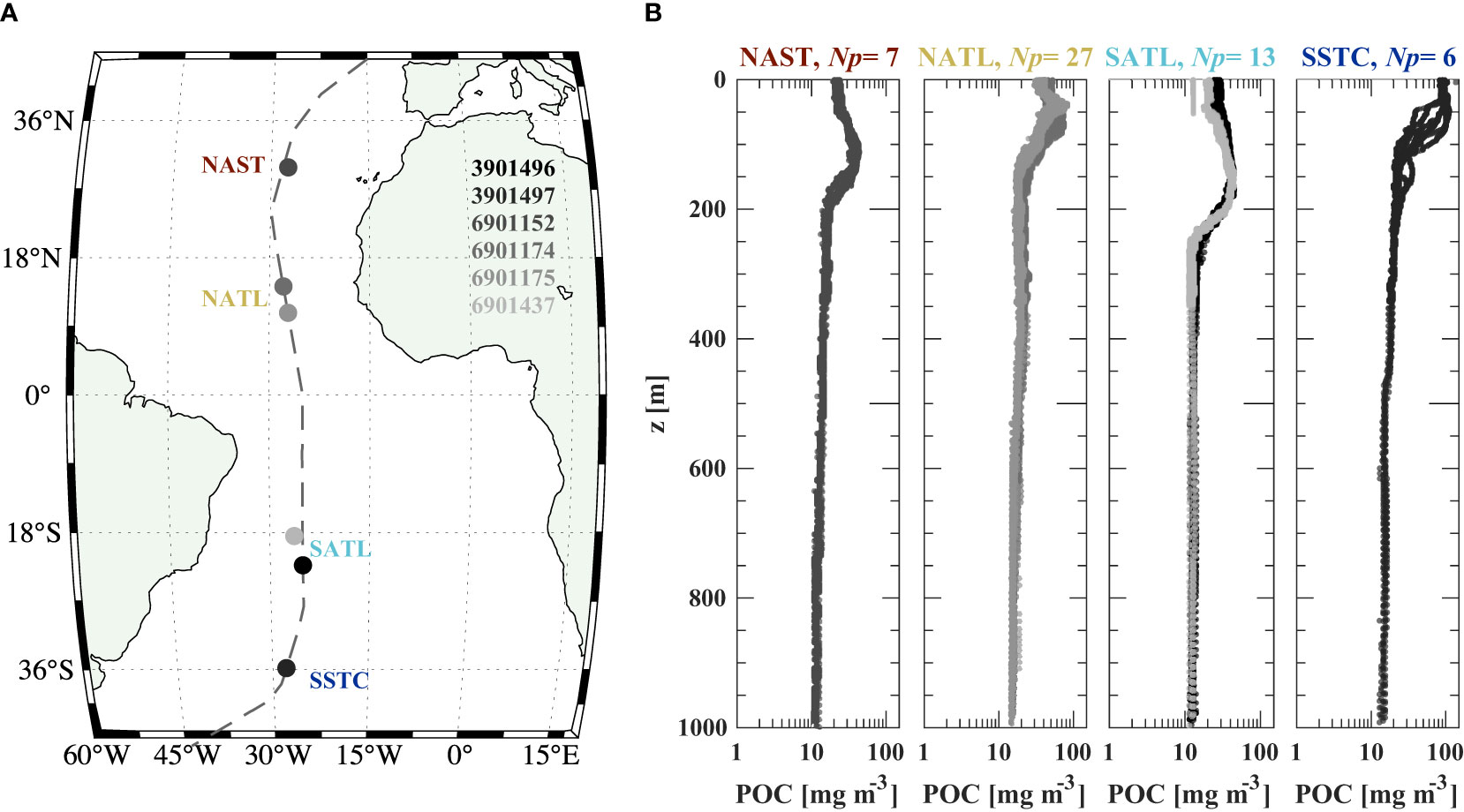
Figure 12 (A) Map of BGC-Argo floats (circles) coincident with the AMT-24 cruise (dashed line) for 24 September – 1 November, 2014. World Meteorological Organization IDs of floats are displayed, and ecological provinces are marked; North Atlantic Subtropical Gyre (NAST), North Atlantic Tropical Gyre (NATL), South Atlantic Gyre (SATL), and South Subtropical Convergence (SSTC). (B) Vertical profiles of POC estimated from Model B of the current study (Table 3; λ = 700 nm, full dataset of surface and subsurface samples). Profiles are grouped by ecological province and number of profiles (Np) is provided.

In Figure 13, we present the statistical distributions of POC estimations from float data within the epipelagic and mesopelagic zones of each ecological province. Estimations of POC from BGC-Argo floats using approaches described by Galí et al. (2022), referred to as Ga22, and Cetinić et al. (2012), referred to as Ce12, are also shown. Overall, all three approaches (i.e., Ko23, Ga22, and Ce12) reproduce the general trend of largest POC values in the SSTC (Figure 13A). Most Ko23 estimates in the epipelagic zone are within the values from Sandoval et al. (2022), except for the North and South Atlantic Tropical Gyres (NATL and SATL) where Ko23 tends to provide larger estimates of POC (Figure 13A). Importantly, the SATL province is large spanning approximately 5°–35° S in latitude and POC measurements by Sandoval et al. (2022) are based on only 2–4 discrete depths in the epipelagic zone. In the SATL province, the median POC from Ko23 is 33 mg m^-3 and we note that similar values (22–28 mg m^-3) were observed by Sandoval et al. (2022) near the float locations. Similarly in the NATL province, the highest values reported by Sandoval et al. (2022) were found near the float locations (35–46 mg m^-3), which are similar to the 50^th to 75^th percentile POC values from Ko23 of 37–46 mg m^-3. When considering Ga22 and Ce12 results, we find that both estimates are generally in agreement with the data from Sandoval et al. (2022) (Figure 13A). In summary, all epipelagic estimates of POC from Ko23, Ga22, and Ce12 are 35 ± 13 mg m^-3, 22 ± 16 mg m^-3, and 17 ± 9 mg m^-3, respectively, while reported values from Sandoval et al. (2022) are 18 ± 9 mg m^-3. Note that Sandoval et al. (2022) report median ± 1 robust standard deviation determined as half the difference between the 84^th and 16^th percentiles, and we report the same statistical measures.

Figure 13

Figure 13 Summary of POC values within the (A) epipelagic (z ≤ 200 m) and (B) mesopelagic (200< z < 500 m) zones using nonparametric boxplots derived from float data in Figure 12. Lower and upper portions of boxes represent 25^th and 75^th percentile values while central circles denote median values and whiskers denote range. Results are displayed for the Ko23 algorithm from the current study as well as the Ga22 and Ce12 algorithms from Galí et al. (2022) and Cetinić et al. (2012), respectively (see section 2.6 for more details). Small horizontal black lines are shown for Ko23 data which represent median values of all lower or upper prediction bounds (two-tailed, α = 0.125). An additional diamond marker is shown for Ko23 estimates which represents median values after removal of a background signal (i.e., b_bp^Δ) determined as the 5^th percentile of b_bp values at a depth of 850–900 m. Reference data are shown for each ecological province using the median value (solid horizontal colored line) ± 1 standard deviation (shaded region) as provided in Sandoval et al. (2022).

In the mesopelagic zone, all approaches also reproduce the general trend of largest POC values in SSTC and second largest values in NATL (Figure 13B). Ko23 estimates are noticeably higher than Sandoval et al. (2022) values by about a factor of two, while Ga22 yields somewhat lower and Ce12 somewhat higher values than the median values of each ecological province reported in Sandoval et al. (2022) (Figure 13B). It is worth noting that the majority of Ga22 estimates are within the measured values from Sandoval et al. (2022). When considering all mesopelagic estimates of POC, Ko23, Ga22, and Ce12 are 19 ± 3.5 mg m^-3, 6.7 ± 2.3 mg m^-3, and 10 ± 2.9 mg m^-3, respectively, while reported values from Sandoval et al. (2022) are 7 ± 2 mg m^-3. It is notable that POC values exceeding 10 mg m^-3 and extending even above 20 mg m^-3 have been previously measured at mesopelagic depths. For example, during the ANT-XXIII/1 cruise in the Atlantic Ocean described in Stramski et al. (2008), POC measurements for the depth range 200-500 m ranged from 11 to 41 mg m^-3 with an average of about 18 mg m^-3. These data were obtained with the same POC method as our present algorithm development dataset (i.e., no DOC-adsorption correction and filtration of sufficiently large volumes). We also note that these mesopelagic data are not reported in Stramski et al. (2008) but are available through NASA’s SeaWiFS Bio-optical Archive and Storage System (SeaBASS, https://seabass.gsfc.nasa.gov/).

Although there are some expected uncertainties from the above analysis (e.g., discrete water measurements lack vertical coverage of BGC-Argo floats and there are no precise match-ups with regards to time of sampling), we found that Ko23 estimates are significantly higher compared with estimates from Sandoval et al. (2022), especially in the mesopelagic zone. Although our algorithm development dataset did not include any mesopelagic samples, we believe that this discrepancy is mostly explainable by a combination of three factors: (1) the influence of DOC adsorption, (2) the influence of backscattering by small colloidal particles, and (3) general uncertainties when particulate signals are very low. Sandoval et al. (2022) applied a DOC-adsorption correction by use of two stacked GF/F filters, where the signal of any material retained on the lower filter is subtracted from the upper filter to estimate POC. We note here that it has been shown that Chla-containing particles can be retained on GF/F filters during filtration of GF/F filtrate, suggesting that some material which passes through a GF/F should be added back to the first filter for a more accurate representation of total particulate matter (e.g., Taguchi and Laws, 1988; Stramski, 1990). As discussed previously in section 4.3, we intentionally did not include DOC-adsorption subtraction from POC in our algorithm development dataset because b_bp is indeed influenced by small-sized colloidal particles which are mostly missed by GF/F filters. For example, Zhang et al. (2020) found that in the very clear North Pacific Ocean, approximately 15–50% of b_bp(517) can be attributed to colloids in GF/F filtrate and this proportion of b_bp from colloids was highest for subsurface samples deeper than 100 m. Thus, in the mesopelagic zone, it is reasonable to expect that small colloids are an important and, at times, dominant contributor to b_bp and this may, at least partly, explain why Ko23 estimates of POC are consistently larger than Sandoval et al. (2022) estimates in the mesopelagic zone (Figure 13B). We reiterate here that we believe that Ko23 estimates are more representative of total POC including some contributions from small colloidal material due to the purposeful omission of an attempt at DOC-adsorption correction, whereas Sandoval et al. (2022) estimates are likely more representative of POC associated with particles retained on GF/F filters.

As an attempt to examine what optically-based POC estimates would be without influence of small-sized colloids, we reprocessed the BGC-Argo data with the removal of a background signal of b_bp. This background (referred to as b_bp^Δ) was determined as the 5^th percentile of b_bp values at 850–900 m depth from each float and is considered a combination of a quasi-constant backscattering background and uncertainty in manufacturer dark-counts (Poteau et al., 2017; Briggs et al., 2020). For the six floats included in our analysis, b_bp^Δ was 1.5–2.4 × 10^-4 m^-1. Importantly, we note that b_bp^Δ is reasonable in comparison to the so-called “background” b_bp(517) signal from particles smaller than 0.2 µm and 0.7 µm found by Zhang et al. (2020); 2.3 × 10^-4 (± 25%) m^-1 and 3.5 × 10^-4 (± 26%) m^-1, respectively, recalling that b_bp^Δ in the current study is determined with λ = 700 nm and thus should be somewhat lower. In Figure 13, we also report median values (diamond markers) of Ko23 estimates of POC for each province determined using b_bp with the contribution from b_bp^Δ removed and we believe these adjusted estimates are more representative of POC without the contribution of small colloids and, thus, more similar to POC corrected for DOC-adsorption. With this adjustment, we find overall better agreement of Ko23 estimates with Sandoval et al. (2022) reported values, especially in the mesopelagic zone (Figure 13B). The removal of b_bp^Δ decreases POC in the mesopelagic zone by about 3–15 mg m^-3 for Ko23, 3–5 mg m^-3 for Ga22, and 5–8 mg m^-3 for Ce12. However, the estimates from Ga22 and Ce12 with removal of b_bp^Δ would become unrealistically low in the mesopelagic zone. We recall that Ga22 relies on relatively little observational data to generate the expected POC/b_bp ratio in the mesopelagic zone, relying on data from Cetinić et al. (2012) which, importantly, did include a DOC-adsorption correction resulting in some negative POC data below 200 m (Bol et al., 2018). The POC/b_bp ratios from Ga22 decrease with depth, but typically were 20471 ± 3481 mg C m^-2 for mesopelagic depths considered (a factor of about 2 lower than the surface), although Bol et al. (2018) showed that these ratios in the mesopelagic zone can be less than 0 mg C m^-2 to over 40000 mg C m^-2. The decrease in POC/b_bp with depth could be explained by changes in particle composition and size distribution, as well as the increased influence of colloidal scattering to b_bp with minimal increase to POC retained on GF/F filters. In conclusion, we do not recommend removing b_bp^Δ from b_bp in application studies aimed at examining total POC estimates from optical measurements, rather we see the influence of small-sized colloids to b_bp as a reasonable factor contributing to differences between Ko23 estimates of POC and the DOC-corrected Sandoval et al. (2022) observations in the mesopelagic zone, while we encourage careful consideration of various influences to and definitions of “particulate” signals. There is also a need for consistency in definition and interpretation of POC estimates obtained from measurements and/or modeling.

It must also be recognized that the mesopelagic zone is characterized by generally low values of both POC and particulate backscattering which approach the limits of methodological and instrument sensitivity, and thus both measurements in this depth range are subject to a high risk of large relative uncertainties. For POC values typically observed at mesopelagic depths, measurements reported in different studies will be considerably affected by the POC measurement protocol employed and subject to high relative uncertainties in experimental determination (e.g., Moran et al., 1999; Gardner et al., 2003). In addition, there is a need to develop improvements of POC measurement methodology to provide better estimates of total POC associated with all suspended particles, including small colloidal particles which can have a strong contribution to ocean optical properties (Organelli et al., 2018; Stramski and Woźniak, 2005; Zhang et al., 2020). Determinations of the particulate backscattering coefficient in many oceanic environments are also strongly influenced by instrument sensitivity and relatively large contributions of pure water and other background to the measured scattering signal. In Figure 14, we present an analysis of the sources of “background” signal to optical backscattering measured by the BGC-Argo float sensors. In the epipelagic zone, b_bp^Δ corresponds to roughly 35% ± 16% of b_bp, while the backscattering coefficient of seawater b_bw and b_bp^Δ together account for 61% ± 15% of the total backscattering coefficient b_b (Figure 14A). These proportions increase noticeably in the mesopelagic zone where such “background” signals are often over 70% and sometimes over 90% of the backscattering coefficient (Figure 14B). It is important to recognize that investigating particulate backscattering in the mesopelagic zone is often at the sensitivity limit of available instrumentation. Although the types of sensors on BGC-Argo floats typically have resolution of approximately 0.5–3 × 10^-5 m^-1 per detector count, dark counts are typically around 30–50 and sufficient signal is required for accuracy. In addition, there are various sources of instrument uncertainty that are important to consider, e.g., factory dark-counts, drift in scale factor, and so-called χ-factor used to estimate b_bp from a single backscattering angle (which may vary with large changes in the particle size distribution). We also recall that Poteau et al. (2017) showed that b_bp^Δ had significant differences for different sensors (e.g., MCOMS vs. ECO-Triplet) and suggest that significant deviation in b_bp^Δ is expected from extraordinary processes or malfunctioning sensor, which further emphasizes that caution must be taken when investigating such low particulate scattering signals. Further work is needed to examine performance of optical backscattering algorithms to estimate POC in the mesopelagic zone, and with varying sensors, especially those on BGC-Argo floats and gliders.

Figure 14

Figure 14 Histograms of various sources of background signal to optical backscattering measured by the BGC-Argo floats shown in Figure 12 for the (A) epipelagic (z ≤ 200 m) and (B) mesopelagic (200< z < 500 m) zones. The backscattering coefficient of pure water and dissolved salts b_bw was determined as a function of salinity and temperature based on Zhang and Hu (2009). The total backscattering coefficient b_b refers to the sum of b_bp and b_bw. b_bp^Δ was determined as the 5^th percentile of b_bp values at a depth of 850–900 m from each float.

5 Concluding remarks

In the current study, we revised univariate and multivariable algorithms presented recently in Koestner et al. (2022) for improved estimations of POC from optical backscattering and chlorophyll-a measurements using a relatively large dataset covering various contrasting water types, including surface and subsurface waters from the Atlantic, Pacific, Arctic, and Southern Oceans. We provide useful refinements to the algorithms including improved model coefficients and prediction uncertainty using a larger and updated dataset compared to that in Koestner et al. (2022). We also provide algorithms for several wavelengths used commonly in observations to derive b_bp, and specifically formulated algorithms for application with near-surface observations. The multivariable algorithm (Model B) can produce reliable estimates of POC across a range of highly contrasting waters in terms of location of sampling and particle and optical properties with noteworthy improvements compared with a typical univariate b_bp-based algorithm (Model B). We determined that the multivariable algorithm has limited sensitivity to uncertainties in both b_bp and Chla. Finally, we also examined performance of several algorithms to estimate POC using our dataset as well as a dataset consisting of optical measurements from BGC-Argo floats and traditional POC measurements collected during a coincident research cruise in the Atlantic Ocean.

The formulation of algorithms based exclusively on near-surface observations will be useful for satellite applications, especially as capabilities to derive b_bp and Chla from ocean color reflectance measurements improve (e.g., Loisel et al., 2018; O’Reilly and Werdell, 2019), as well as b_bp more directly from lidar observations (e.g., Lu et al., 2021; Behrenfeld et al., 2022). We expect some challenges for estimating POC using Model B based on the combination of satellite observations of b_bp and Chla, e.g., reliability of b_bp from lidar or ocean color inversions (Werdell et al., 2018; Behrenfeld et al., 2022). In comparison, POC algorithms which rely on estimation of POC in surface ocean waters directly from satellite-derived ocean reflectance have been recently improved and validated for applications in open-ocean pelagic environments that dominate the global ocean as well as other environments including coastal waters that exhibit bio-optical properties consistent with those found typically in the open ocean (e.g., Stramski et al., 2022; Joshi et al., 2023). There is also potential for further advancements in applications across diverse water bodies including optically-complex waters through development of adaptive POC algorithms which explicitly account for variations in particulate composition in terms of varying proportions of organic vs. mineral particles (Stramski et al., 2023). Nonetheless, one potential advantage of the proposed multivariable approach involving b_bp as a predictive variable for POC regards the decoupling of POC estimates from optically-derived Chla estimates. Historically, such coupling has been associated with satellite estimates of POC and Chla retrieved from similar spectral bands of ocean reflectance (e.g., Gordon et al., 1983; Stramski et al., 2008; Evers-King et al., 2017; O’Reilly and Werdell, 2019; Stramski et al., 2022). Although Chla is included as input into our multivariable b_bp–based algorithms and there should be some natural correlation between Chla and POC in many oceanic environments, the multivariable Model B can reasonably produce large variability in POC (factors of about 2–10) for the same values of Chla depending on b_bp and particle composition. Thus, further exploring application of this multivariable algorithm to remote sensing observations is worthwhile.

Notwithstanding satellite or other above-water remote sensing observations, we consider a main use-case of multivariable model B in conjunction with in situ measurements such as from BGC-Argo floats or autonomous gliders which typically make measurements of both b_bp and chlorophyll-a fluorescence. We expect that the algorithms can be particularly useful for assessments of temporal and spatial (including vertical) distributions of POC in the ocean (Johnson et al., 2009; Biogeochemical-Argo Planning Group, 2016; Roemmich et al., 2019). We acknowledge, however, that further validation of algorithm performance during various time frames, seasons, and depths outside the algorithm development dataset is desirable. Currently, estimates of POC with BGC-Argo floats rely almost exclusively on univariate b_bp algorithms (e.g., Dall’Olmo and Mork, 2014; Johnson et al., 2017; Xing et al., 2020; Wang and Fennel, 2023), or approaches which rely on adjustments to account for vertical and regional variability in the relationship between b_bp and POC (Bol et al., 2018; Galí et al., 2022). We also believe that multivariable Model B can be particularly useful for assessments of POC with optical measurements from autonomous gliders in nearshore or coastal waters which are often not surveyed by BGC-Argo floats and are optically-complex containing non-negligible contributions of non-phytoplankton material.

We believe that it is possible to develop relatively robust optical algorithms which can work across diverse environments by incorporating mechanistic aspects of the interactions of light and seawater constituents. The use of particle composition parameter in our multivariable approach of Model B is meant to introduce a mechanistic aspect to the b_bp-based POC algorithm which can pave the way for applications across diverse water bodies regardless of regional or seasonal variations in environmental conditions. Although the current multivariable algorithm is expected to provide reasonable estimates of POC for a variety of water types within the epipelagic zone and extending potentially also to deeper mesopelagic depths (Figure 13), it is important to recognize a need for new sensors and approaches. For example, while targeting POC at deeper depths with no active phytoplankton growth, it will be useful to account for particulate composition that does not just rely on chlorophyll-a fluorescence. In addition, the effects of particle size distribution on optical properties may also be important to consider. The potential new sensors may take advantage of specific polarization and angular scattering properties which are indicative of particle size distribution as well as compositional properties such as the ratio of particulate organic carbon to total suspended particulate matter (Koestner et al., 2020; Koestner et al., 2021). With advancements targeting the improved estimation of POC throughout the ocean water column including the mesopelagic and deeper depths, we expect to better understand the natural ability of the biological carbon pump to sequester carbon in the deep ocean (e.g., Brewin et al., 2021).

Data availability statement

The raw data supporting the conclusions of this article will be made available by the authors, without undue reservation. POC algorithms are available at https://github.com/DanielKoestner/Koestner_2023_POC.

Author contributions

DK, DS, and RR conceptualized the study with DK performing the bulk of the algorithm development and validation. DK wrote the first draft of the manuscript. All authors contributed to the article and approved the submitted version.

Funding

This study was supported by the European Union’s Horizon 2020 Framework Programme for Research and Innovation under the Marie Skłodowska-Curie grant agreement No. 101034309. Partial support was provided by the U.S. National Aeronautics and Space Administration (Grants NNX17AI72G, 80NSSC18K0956, and 80NSSC21K0700).

Acknowledgments

POC analysis of seawater samples was done at the Marine Science Institute, University of California Santa Barbara. We express our gratitude to Dr. Paul Lerner for support in the development of BGC-Argo processing codes. Thanks to all science crew and ship operators who facilitated collection of data used in this study. We also thank Dr. Martí Galí and Jordon Scott Beckler for their valuable comments on the manuscript.

Conflict of interest

The authors declare that the research was conducted in the absence of any commercial or financial relationships that could be construed as a potential conflict of interest.

Publisher’s note

All claims expressed in this article are solely those of the authors and do not necessarily represent those of their affiliated organizations, or those of the publisher, the editors and the reviewers. Any product that may be evaluated in this article, or claim that may be made by its manufacturer, is not guaranteed or endorsed by the publisher.

References

Ackleson S. G., Cullen J. J., Brown J., Lesser M. P. (1990). Some changes in the optical properties of marine phytoplankton in response to high light intensity. Proc. SPIE 1302, Ocean Optics X, 238–249. doi: 10.1117/12.21449

CrossRef Full Text | Google Scholar

Balch W. M., Bowler B. C., Drapeau D. T., Poulton A. J., Holligan P. M. (2010). Biominerals and the vertical flux of particulate organic carbon from the surface ocean. Geophys. Res. Lett. 37, L22605. doi: 10.1029/2010GL044640

CrossRef Full Text | Google Scholar

Barbieux M., Uitz J., Bricaud A., Organelli E., Poteau A., Schmechtig, et al. (2018). Assessing the variability in the relationship between the particulate backscattering coefficient and the chlorophyll a concentration from a global Biogeochemical-Argo database. J. Geophys. Res. 123, 1229–1250. doi: 10.1002/2017JC013030

CrossRef Full Text | Google Scholar

Behrenfeld M. J., Hu Y., Bisson K. M., Lu X., Westberry T. K. (2022). Retrieval of ocean optical and plankton properties with the satellite Cloud-Aerosol Lidar with Orthogonal Polarization (CALIOP) sensor: Background, data processing, and validation status. Remote Sens. Environ. 281, 113235. doi: 10.1016/j.rse.2022.113235

CrossRef Full Text | Google Scholar

Behrenfeld M. J., Hu Y., Hostetler C. A., Dall'Olmo G., Rodier S. D., Hair J. W., et al. (2013). Space-based lidar measurements of global ocean carbon stocks. Geophys. Res. Lett. 40, 4355–4360. doi: 10.1002/grl.50816

CrossRef Full Text | Google Scholar

Biogeochemical-Argo Planning Group. (2016). The scientific rationale, design and implementation plan for a Biogeochemical-Argo float array. Eds. Johnson K., Claustre H. doi: 10.13155/46601

CrossRef Full Text | Google Scholar

Bishop J. K. B. (1999). Transmissometer measurement of POC. Deep-Sea. Res. I. 46, 353–369. doi: 10.1016/S0967-0637(98)00069-7

CrossRef Full Text | Google Scholar

Bisson K. M., Boss E., Werdell P. J., Ibrahim A., Behrenfeld M. J. (2021). Particulate backscattering in the global ocean: A comparison of independent assessments. Geophys. Res. Lett. 48, e2020GL090909. doi: 10.1029/2020GL090909

PubMed Abstract | CrossRef Full Text | Google Scholar

Bol R., Henson S. A., Rumyantseva A., Briggs N. (2018). High-frequency variability of small-particle carbon export flux in the Northeast Atlantic. Glob. Biogeochem. Cycles. 32, 1803–1814. doi: 10.1029/2018GB005963

CrossRef Full Text | Google Scholar

Boss E., Pegau W. (2001). Relationship of light scattering at an angle in the backward direction to the backscattering coefficient. Appl. Opt. 40, 5503–5507. doi: 10.1364/AO.40.005503

PubMed Abstract | CrossRef Full Text | Google Scholar

Boss E., Pegau W. S., Lee M., Twardowski M., Shybanov E., Korotaev G., et al. (2004). Particulate backscattering ratio at LEO 15 and its use to study particle composition and distribution. J. Geophys. Res. 109, C01014. doi: 10.1029/2002JC001514

CrossRef Full Text | Google Scholar

Boss E. S., Collier R., Pegau W. S., Larson G., Fennel K. (2007). “Measurements of spectral optical properties and their relation to biogeochemical variables and processes in Crater Lake, Crater Lake National Park, OR,” in Long-term Limnological Research and Monitoring at Crater Lake, Oregon. Developments in Hydrobiology, vol. 191. (Dordrecht: Springer), 149–159. doi: 10.1007/978-1-4020-5824-0_9

CrossRef Full Text | Google Scholar

Boyd P. W., Trull T. W. (2007). Understanding the export of biogenic particles in oceanic waters: Is there consensus? Prog. Oceanogr. 72, 276–312. doi: 10.1016/j.pocean.2006.10.007

CrossRef Full Text | Google Scholar

Brewin R. J. W., Sathyendranath S., Platt T., Bouman H., Ciavatta S., Dall'Olmo G., et al. (2021). Sensing the ocean biological carbon pump from space: A review of capabilities, concepts, research gaps and future developments. Earth Sci. Rev. 217, 103604. doi: 10.1016/j.earscirev.2021.103604

CrossRef Full Text | Google Scholar

Briggs N., Dall’Olmo G., Claustre H. (2020). Major role of particle fragmentation in regulating biological sequestration of CO2 by the oceans. Science 367, 791–793. doi: 10.1126/science.aay1790

PubMed Abstract | CrossRef Full Text | Google Scholar

Buiteveld H., Hakvoort J. H.M., Donze M. (1994). Optical properties of pure water. Proc. SPIE 2258, Ocean Optics XII. doi: 10.1117/12.190060

CrossRef Full Text | Google Scholar

Cetinić I., Perry M. J., Briggs N. T., Kallin E., D'Asaro E. A., Lee C. M. (2012). Particulate organic carbon and inherent optical properties during 2008 North Atlantic Bloom Experiment. J. Geophys. Res. 117, C06028. doi: 10.1029/2011JC007771

CrossRef Full Text | Google Scholar

Churnside J. H., Tatarskii V. V., Wilson J. J. (1998). Oceanographic lidar attenuation coefficients and signal fluctuations measured from a ship in the Southern California Bight. Appl. Opt. 47, 3105–3112. doi: 10.1364/AO.37.003105

CrossRef Full Text | Google Scholar

Claustre H., Morel A., Babin M., Cailliau C., Marie D., Marty J.-C., et al. (1999). Variability in particle attenuation and chlorophyll fluorescence in the Tropical Pacific: Scales, patterns, and biogeochemical implications. J. Geophys. Res. 104, 3401–3422. doi: 10.1029/98JC01334

CrossRef Full Text | Google Scholar

Dall’Olmo G., Mork K. J. (2014). Carbon export by small particles in the Norwegian Sea. Geophys. Res. Lett. 41, 2921–2927. doi: 10.1002/2014GL059244

CrossRef Full Text | Google Scholar

Erickson Z. K., Cetinić I., Zhang X., Boss E., Werdell P. J., Freeman S., et al. (2022). Alignment of optical backscatter measurements from the EXPORTS Northeast Pacific Field Deployment. Elem. Sci. Anth. 10, 1. doi: 10.1525/elementa.2021.00021

CrossRef Full Text | Google Scholar

Evers-King H., Martinez-Vicente V., Brewin R. J. W., Dall’Olmo G., Hickman A. E., Jackson T., et al. (2017). Validation and intercomparison of ocean color algorithms for estimating particulate organic carbon in the oceans. Front. Mar. Sci. 4, 251. doi: 10.3389/fmars.2017.00251

CrossRef Full Text | Google Scholar

Fay A. R., McKinley G. A. (2014). Global open-ocean biomes: mean and temporal variability. Earth System. Sci. Data 6 (2), 273–284. doi: 10.5194/essd-6-273-2014

CrossRef Full Text | Google Scholar

Friedlingstein P., O’Sullivan M., Jones M. W., Andrew R. M., Gregor L., Hauck J., et al. (2022). Global carbon budget 2022. Earth Syst. Sci. Data 14, 4811–4900. doi: 10.5194/essd-14-4811-2022

CrossRef Full Text | Google Scholar

Galí M., Falls M., Claustre H., Aumont O., Bernardello R. (2022). Bridging the gaps between particulate backscattering measurements and modeled particulate organic carbon in the ocean. Biogeosciences 19, 1245–1275. doi: 10.5194/bg-19-1245-2022

CrossRef Full Text | Google Scholar

Gardner W. D., Mishonov A. V., Richardson M. J. (2006). Global POC concentrations from in-situ and satellite data. Deep. Sea. Res. II. 53, 718–740. doi: 10.1016/j.dsr2.2006.01.029

CrossRef Full Text | Google Scholar

Gardner W. D., Richardson M. J., Carlson C. A., Hansell D., Mishonov A. V. (2003). Determining true particulate organic carbon: bottles, pumps and methodologies. Deep. Sea. Res. II. 50, 655–674. doi: 10.1016/S0967-0645(02)00589-1

CrossRef Full Text | Google Scholar

Gardner W. D., Walsh I. D., Richardson M. J. (1993). Biophysical forcing of particle production and distribution during a spring bloom in the North Atlantic. Deep. Sea. Res. II. 40, 171–195. doi: 10.1016/0967-0645(93)90012-C

PubMed Abstract | CrossRef Full Text | Google Scholar

Getzewich B. J., Vaughan M. A., Hunt W. H., Avery M. A., Powell K. A., Tackett J. L., et al. (2018). CALIPSO lidar calibration at 532 nm: Version 4 daytime algorithm. Atmos. Meas. Tech. 11, 6309–6326. doi: 10.5194/amt-11-6309-2018

CrossRef Full Text | Google Scholar

Gordon H. R., Clark D. K., Brown J. W., Brown O. B., Evans R. H., Broenkow W. W. (1983). Phytoplankton pigment concentrations in the Middle Atlantic Bight: comparison of ship determinations and CZCS estimates. Appl. Opt. 22, 20–36. doi: 10.1364/AO.22.000020

PubMed Abstract | CrossRef Full Text | Google Scholar

Intergovernmental Oceanographic Commission. (1994). Protocols for the Joint Global Ocean Flux Study (JGOFS) Core Measurements. Intergovernmental Oceanographic Commission, Scientific Committee on Oceanic Research, Manuals and Guides No. 29 (Paris: UNESCO-IOC).

Google Scholar

IOCCG Protocol Series. (2021). Particulate Organic Matter Sampling and Measurement Protocols: Consensus Towards Future Ocean Color Missions. Chaves J. E., Cetinić I., Dall’Olmo G., Estapa M., Gardner W., Goñi M., et al. IOCCG Ocean Optics and Biogeochemistry Protocols for Satellite Ocean Colour Sensor Validation Vol. 6.0 (Dartmouth, NS, Canada: IOCCG).

Google Scholar

Jamet C., Ibrahim A., Ahmad Z., Angelini F., Babin M., Behrenfeld M. J., et al. (2019). Going beyond standard ocean color observations: Lidar and polarimetry. Front. Mar. Sci. 6, 251. doi: 10.3389/fmars.2019.00251

CrossRef Full Text | Google Scholar

Johnson K. S., Berelson W. M., Boss E. S., Chase Z., Claustre H., Emerson S. R., et al. (2009). Observing biogeochemical cycles at global scales with profiling floats and gliders: Prospects for a global array. Oceanography 22, 216–225. doi: 10.5670/oceanog.2009.81

CrossRef Full Text | Google Scholar

Johnson K. S., Plant J. N., Coletti L. J., Jannasch H. W., Sakamoto C. M., Riser S. C., et al. (2017). Biogeochemical sensor performance in the SOCCOM profiling float array. J. Geophys. Res. 122, 6416–6436. doi: 10.1002/2017jc012838

CrossRef Full Text | Google Scholar

Joshi I. D., Stramski D., Reynolds R. A., Robinson D. H. (2023). Performance assessment and validation of ocean color sensor-specific algorithms for estimating the concentration of particulate organic carbon in oceanic surface waters from satellite observations. Remote Sens. Environ. 286, 113417. doi: 10.1016/j.rse.2022.113417

CrossRef Full Text | Google Scholar

Koestner D., Stramski D., Reynolds R. A. (2018). Measurements of the volume scattering function and the degree of linear polarization of light scattered by contrasting natural assemblages of marine particles. Appl. Sci. 8 (12), 2690. doi: 10.3390/app8122690

CrossRef Full Text | Google Scholar

Koestner D., Stramski D., Reynolds R. A. (2020). Polarized light scattering measurements as a means to characterize particle size and composition of natural assemblages of marine particles. Appl. Opt. 59, 8314–8334. doi: 10.1364/AO.396709

PubMed Abstract | CrossRef Full Text | Google Scholar

Koestner D., Stramski D., Reynolds R. A. (2021). Characterization of suspended particulate matter in contrasting coastal marine environments with angle-resolved polarized light scattering measurements. Appl. Opt. 60, 11161–11179. doi: 10.1364/AO.441226

PubMed Abstract | CrossRef Full Text | Google Scholar

Koestner D., Stramski D., Reynolds R. A. (2022). A multivariable empirical algorithm for estimating particulate organic carbon concentration in marine environments from optical backscattering and chlorophyll-a measurements. Front. Mar. Sci. 9, 941950. doi: 10.3389/fmars.2022.941950

CrossRef Full Text | Google Scholar

Lee Z., Carder K. L., Arnone R. A. (2002). Deriving inherent optical properties from water color: a multiband quasi-analytical algorithm for optically deep waters. Appl. Opt. 41, 5755–5772. doi: 10.1364/AO.41.005755

PubMed Abstract | CrossRef Full Text | Google Scholar

Loisel H., Nicolas J.-M., Deschamps P.-Y., Frouin R. (2002). Seasonal and inter-annual variability of particulate organic matter in the global ocean. Geophys. Res. Lett. 29, 2196. doi: 10.1029/2002GL015948

CrossRef Full Text | Google Scholar

Loisel H., Stramski D. (2000). Estimation of the inherent optical properties of natural waters from the irradiance attenuation coefficient and reflectance in the presence of Raman scattering. Appl. Opt. 39, 3001–3011. doi: 10.1364/AO.39.003001

PubMed Abstract | CrossRef Full Text | Google Scholar

Loisel H., Stramski D., Dessailly D., Jamet C., Li L., Reynolds R. A. (2018). An inverse model for estimating the optical absorption and backscattering coefficients of seawater from remote-sensing reflectance over a broad range of oceanic and coastal marine environments. J. Geophys. Res. 123, 2141–2171. doi: 10.1002/2017JC013632

CrossRef Full Text | Google Scholar

Longhurst A. R. (2007). “Chapter 9 - The Atlantic Ocean,” in Ecological Geography of the Sea, 2nd ed. Ed. Longhurst A. R. (Burlington: Academic Press), 131–273.

Google Scholar

Lu X., Hu Y., Yang Y. (2019). “Ocean subsurface study from ICESat-2 mission,” in Photonics & Electromagnetics Research Symposium - Fall (PIERS - Fall). 910–918(Xiamen, China). doi: 10.1109/PIERS-Fall48861.2019.9021802

CrossRef Full Text | Google Scholar

Lu X., Hu Y., Yang Y., Neumann T., Omar A., Baize R., et al. (2021). New ocean subsurface optical properties from space lidars: CALIOP/CALIPSO and ATLAS/ICESat-2. Earth Space. Sci. 8, e2021EA001839. doi: 10.1029/2021EA001839

CrossRef Full Text | Google Scholar

McKinna L. I. W., Cetinić I., Werdell P. J. (2021). Development and validation of an empirical ocean color algorithm with uncertainties: A case study with the particulate backscattering coefficient. J. Geophys. Res. 126, e2021JC017231. doi: 10.1029/2021JC017231

PubMed Abstract | CrossRef Full Text | Google Scholar

Middelburg J. J. (2019). Marine Carbon Biogeochemistry: A Primer for Earth System Scientists (Berlin, Germany: Springer Nature).

Google Scholar

Moran S. B., Charette M. A., Pike S. M., Wicklund C. A. (1999). Differences in seawater particulate organic carbon concentration in samples collected using small-and large-volume methods: the importance of DOC adsorption to the filter blank. Mar. Chem. 67 (1-2), 33–42. doi: 10.1016/S0304-4203(99)00047-X

CrossRef Full Text | Google Scholar

Morel A., Bricaud A. (1981). Theoretical results concerning light absorption in a discrete medium, and application to specific absorption of phytoplankton. Deep. Sea. Res. 28A, 1375–1393. doi: 10.1016/0198-0149(81)90039-X

PubMed Abstract | CrossRef Full Text | Google Scholar

Neukermans G., Loisel H., Meriaux X., Astoreca R., McKee D. (2012). In situ variability of mass-specific beam attenuation and backscattering of marine particles with respect to particle size, density, and composition. Limnol. Oceanogr. 57, 124–144. doi: 10.4319/lo.2012.57.1.0124

CrossRef Full Text | Google Scholar

Novak M. G., Cetinić I., Chaves J. E., Mannino A. (2018). The adsorption of dissolved organic carbon onto glass fiber filters and its effect on the measurement of particulate organic carbon: A laboratory and modeling exercise. Limnol. Oceanogr. Methods 16 (6), 356–366. doi: 10.1002/lom3.10248

PubMed Abstract | CrossRef Full Text | Google Scholar

Nowicki M., DeVries T., Siegel D. A. (2022). Quantifying the carbon export and sequestration pathways of the ocean's biological carbon pump. Glob. Biogeochem. Cycles. 36 (3), e2021GB007083. doi: 10.1029/2021GB007083

PubMed Abstract | CrossRef Full Text | Google Scholar

O’Reilly J. E., Werdell P. J. (2019). Chlorophyll algorithms for ocean color sensors - OC4, OC5 & OC6. Remote Sens. Environ. 229, 32–47. doi: 10.1016/j.rse.2019.04.021

PubMed Abstract | CrossRef Full Text | Google Scholar

Organelli E., Barbieux M., Claustre H., Schmechtig C., Poteau A., Bricaud A., et al. (2017). Two databases derived from BGC-Argo float measurements for marine biogeochemical and bio-optical applications. Earth Syst. Sci. Data 9, 861–880. doi: 10.5194/essd-9-861-2017

CrossRef Full Text | Google Scholar

Organelli E., Dall’Olmo G., Brewin R. J.W., Tarran G. A., Boss E., Bricaud A. (2018). The open-ocean missing backscattering is in the structural complexity of particles. Nat. Commun. 9, 5439. doi: 10.1038/s41467-018-07814-6

PubMed Abstract | CrossRef Full Text | Google Scholar

Paraekh P., Dutkiewicz S., Follows M. J., Ito T. (2006). Atmospheric carbon dioxide in a less dusty world. Geophys. Res. Lett. 33, L03610. doi: 10.1029/2005GL025098

CrossRef Full Text | Google Scholar

Parsons T. R., Maita Y., Lalli C. M. (1984). A Manual of Chemical and Biological Methods for Seawater Analysis (Oxford, England: Pergamon Press).

Google Scholar

Poteau A., Boss E., Claustre H. (2017). Particulate concentration and seasonal dynamics in the mesopelagic ocean based on the backscattering coefficient measured with Biogeochemical-Argo floats. Geophys. Res. Lett. 44, 6933–6939. doi: 10.1002/2017GL073949

CrossRef Full Text | Google Scholar

Reynolds R. A., Stramski D., Kiefer D. A. (1997). The effect of nitrogen-limitation on the absorption and scattering properties of the marine diatom Thalassiosira pseudonana. Limnol. Oceanogr. 42, 881–892. doi: 10.4319/lo.1997.42.5.0881

CrossRef Full Text | Google Scholar

Reynolds R. A., Stramski D., Neukermans G. (2016). Optical backscattering by particles in Arctic seawater and relationships to particle mass concentration, size distribution, and bulk composition. Limnol. Oceanogr. 61, 1869–1890. doi: 10.1002/lno.10341

CrossRef Full Text | Google Scholar

Roemmich D., Alford M. H., Claustre H., Johnson K., King B., Moum J., et al. (2019). On the future of Argo: A global, full-depth, multi-disciplinary array. Front. Mar. Sci. 6. doi: 10.3389/fmars.2019.00439

CrossRef Full Text | Google Scholar

Roesler C., Uitz J., Claustre H., Boss E., Xing X., Organelli E., et al. (2017). Recommendations for obtaining unbiased chlorophyll estimates from in situ chlorophyll fluorometers: a global analysis of WET Labs ECO sensors. Limnol. Oceanogr. 15, 572–585. doi: 10.1002/lom3.10185

PubMed Abstract | CrossRef Full Text | Google Scholar

Sandoval P. S., Dall'Olmo G., Haines K., Rasse R., Ross J. (2022). Uncertainties of particulate organic carbon concentrations in the mesopelagic zone of the Atlantic Ocean. Open Res. Europe. 1, 43. doi: 10.12688/openreseurope.13395.3

CrossRef Full Text | Google Scholar

Siegel D. A., Buesseler K. O., Behrenfeld M. J., Benitez-Nelson C. R., Boss E., Brzezinski M. A., et al. (2016). Prediction of the export and fate of global ocean net primary production: The EXPORTS science plan. Front. Mar. Sci. 3, 22. doi: 10.3389/fmars.2016.00022

CrossRef Full Text | Google Scholar

Stemmann L., Boss E. (2012). Plankton and particle size and packaging: From determining optical properties to driving the biological pump. Ann. Rev. Mar. Sci. 4, 263–290. doi: 10.1146/annurev-marine-120710-100853

PubMed Abstract | CrossRef Full Text | Google Scholar

Stramska M., Stramski D. (2005). Variability of particulate organic carbon concentration in the north polar Atlantic based on ocean color observations with Sea-viewing Wide Field-of-view Sensor (SeaWiFS). J. Geophys. Res. 110, C10018. doi: 10.1029/2004JC002762

CrossRef Full Text | Google Scholar

Stramski D. (1990). Artifacts in measuring absorption spectra of phytoplankton collected on a filter. Limnol. Oceanogr. 35, 1804–1809. doi: 10.4319/lo.1990.35.8.1804

CrossRef Full Text | Google Scholar

Stramski D., Babin M., Woźniak S. B. (2007). Variations in the optical properties of terrigenous mineral-rich particulate matter suspended in seawater. Limnol. Oceanogr. 52, 2418–2433. doi: 10.4319/lo.2007.52.6.2418

CrossRef Full Text | Google Scholar

Stramski D., Boss E., Bogucki D., Voss K. J. (2004). The role of seawater constituents in light backscattering in the ocean. Prog. Oceanogr. 61 (1), 27–56. doi: 10.1016/j.pocean.2004.07.001

PubMed Abstract | CrossRef Full Text | Google Scholar

Stramski D., Bricaud A., Morel A. (2001). Modeling the inherent optical properties of the ocean based on the detailed composition of the planktonic community. Appl. Opt. 40, 2929–2945. doi: 10.1364/AO.40.002929

PubMed Abstract | CrossRef Full Text | Google Scholar

Stramski D., Constantin S., Reynolds R. A. (2023). Adaptive optical algorithms with differentiation of water bodies based on varying composition of suspended particulate matter: A case study for estimating the particulate organic carbon concentration in the western Arctic seas. Remote Sens. Environ. 286, 113360. doi: 10.1016/j.rse.2022.113360

CrossRef Full Text | Google Scholar

Stramski D., Joshi I., Reynolds R. A. (2022). Ocean color algorithms to estimate the concentration of particulate organic carbon in surface waters of the global ocean in support of a long-term data record from multiple satellite missions. Remote Sens. Environ. 269, 112776. doi: 10.1016/j.rse.2021.112776

CrossRef Full Text | Google Scholar

Stramski D., Kiefer D. A. (1991). Light scattering by microorganisms in the open ocean. Prog. Oceanogr. 28, 343–383. doi: 10.1016/0079-6611(91)90032-H

PubMed Abstract | CrossRef Full Text | Google Scholar

Stramski D., Morel A. (1990). Optical properties of photosynthetic picoplankton in different physiological states as affected by growth irradiance. Deep. Sea. Res. 37, 245–266. doi: 10.1016/0198-0149(90)90126-G

PubMed Abstract | CrossRef Full Text | Google Scholar

Stramski D., Reynolds R. A., Babin M., Kaczmarek S., Lewis M. R., Röttgers R., et al. (2008). Relationships between the surface concentration of particulate organic carbon and optical properties in the eastern South Pacific and eastern Atlantic Oceans. Biogeosciences 5, 171–201. doi: 10.5194/bg-5-171-2008

PubMed Abstract | CrossRef Full Text | Google Scholar

Stramski D., Reynolds R. A., Kahru M., Mitchell B. G. (1999). Estimation of particulate organic carbon in the ocean from satellite remote sensing. Science 285, 239–242. doi: 10.1126/science.285.5425.23

PubMed Abstract | CrossRef Full Text | Google Scholar

Stramski D., Sciandra A., Claustre H. (2002). Effects of temperature, nitrogen, and light limitation on the optical properties of the marine diatom Thalassiosira pseudonana. Limnol. Oceanogr. 47, 392–403. doi: 10.4319/lo.2002.47.2.0392

CrossRef Full Text | Google Scholar

Stramski D., Woźniak S. B. (2005). On the role of colloidal particles in light scattering in the ocean. Limnol. Oceanogr. 50, 1581–1591. doi: 10.4319/lo.2005.50.5.1581

PubMed Abstract | CrossRef Full Text | Google Scholar

Sullivan J. M., Twardowski M. S., Ronald J., Zaneveld V., Moore C. C. (2013). Measuring optical backscattering in water. Light Scattering Reviews 7: Radiative Transfer and Optical Properties of Atmosphere and Underlying Surface (Berlin, Germany: Springer Verlag), 189-224. doi: 10.1007/978-3-642-21907-8_6

CrossRef Full Text | Google Scholar

Taguchi S., Laws E. A. (1988). On the microparticles which pass through glass-fiber filter type GF/F in coastal and open waters. J. Plankton. Res. 10, 999–1008. doi: 10.1093/plankt/10.5.999

CrossRef Full Text | Google Scholar

Twardowski M., Boss E., Macdonald J., Pegau W., Barnard A., Zaneveld J. (2001). A model for estimating bulk refractive index from the optical backscattering ratio and the implication for understanding particle composition in Case I and Case II waters. J. Geophys. Res. 106, 14129–14142. doi: 10.1029/2000JC000404

CrossRef Full Text | Google Scholar

Twardowski M. S., Claustre H., Freeman S. A., Stramski D., Huot Y. (2007). Optical backscattering properties of the "clearest" natural waters. Biogeosciences 4, 1041–1058. doi: 10.5194/bg-4-1041-2007

CrossRef Full Text | Google Scholar

Uitz J., Stramski D., Baudoux A.-C., Reynolds R. A., Wright V. M., Dubranna J., et al. (2010). Variations in the optical properties of a particle suspension associated with viral infection of marine bacteria. Limnol. Oceanogr. 55, 2317–2330. doi: 10.4319/lo.2010.55.6.2317

CrossRef Full Text | Google Scholar

Wang B., Fennel K. (2023). An assessment of vertical carbon flux parameterizations using backscatter data from BGC Argo. Geophys. Res. Lett. 50, e2022GL101220. doi: 10.1029/2022GL101220

CrossRef Full Text | Google Scholar

Werdell P. J., McKinna L. I., Boss E., Ackleson S. G., Craig S. E., Gregg, et al. (2018). An overview of approaches and challenges for retrieving marine inherent optical properties from ocean color remote sensing. Progress in Oceanography 160, 186–212. doi: 10.1016/j.pocean.2018.01.001

CrossRef Full Text | Google Scholar

Woźniak S. B., Meler J., Stoń-Egiert J. (2022). Inherent optical properties of suspended particulate matter in the southern Baltic Sea in relation to the concentration, composition and characteristics of the particle size distribution; new forms of multicomponent parameterizations of optical properties. J. Mar. Sys. 229, 103720. doi: 10.1016/j.jmarsys.2022.103720

CrossRef Full Text | Google Scholar

Woźniak S. B., Stramski D., Stramska M., Reynolds R. A., Wright V. M., Miksic E. Y., et al. (2010). Optical variability of seawater in relation to particle concentration, composition, and size distribution in the nearshore marine environment at Imperial Beach, California. J. Geophys. Res. 115, C08027. doi: 10.1029/2009JC005554

CrossRef Full Text | Google Scholar

Wu J., Lee Z., Xie Y., Goes J., Shang S., Marra J. F., et al. (2021). Reconciling between optical and biological determinants of the euphotic zone depth. J. Geophys. Res. 126, e2020JC016874. doi: 10.1029/2020JC016874

CrossRef Full Text | Google Scholar

Xing X., Claustre H., Blain S., D'Ortenzio F., Antoine D., Ras J., et al. (2012). Quenching correction for in vivo chlorophyll fluorescence acquired by autonomous platforms: A case study with instrumented elephant seals in the Kerguelen region (Southern Ocean). Limnol. Oceanogr. Methods 10, 483–495. doi: 10.4319/lom.2012.10.483

CrossRef Full Text | Google Scholar

Xing X., Claustre H., Boss E., Roesler C., Organelli E., Poteau A., et al. (2017). Correction of profiles of in-situ chlorophyll fluorometry for the contribution of fluorescence originating from non-algal matter. Limnol. Oceanogr. Methods 15, 80–93. doi: 10.1002/lom3.10144

CrossRef Full Text | Google Scholar

Xing X., Wells M. L., Chen S., Lin S., Chai F. (2020). Enhanced winter carbon export observed by BGC-Argo in the Northwest Pacific Ocean. Geophys. Res. Lett. 47, e2020GL089847. doi: 10.1029/2020GL089847

CrossRef Full Text | Google Scholar

Zhang Z., Chen P., Zhong C., Xie C., Sun M., Zhang S., et al. (2023). Chlorophyll and POC in polar regions derived from spaceborne lidar. Front. Mar. Sci. 10, 1050087. doi: 10.3389/fmars.2023.1050087

CrossRef Full Text | Google Scholar

Zhang X., Hu L. (2009). Estimating scattering of pure water from density fluctuation of the refractive index. Opt. Express. 17 (3), 1671–1678. doi: 10.1364/OE.17.001671

CrossRef Full Text | Google Scholar

Zhang X., Hu L., Xiong Y., Huot Y., Gray D. (2020). Experimental estimates of optical backscattering associated with submicron particles in clear oceanic waters. Geophys. Res. Lett. 47, e2020GL087100. doi: 10.1029/2020GL087100

CrossRef Full Text | Google Scholar