Remote sensing of sea surface glacial meltwater on the Antarctic Peninsula shelf

1 Introduction

Sea surface glacial meltwater (SSGM) is a prominent physical feature in the coastal oceans of Antarctica. For instance, at the Western Antarctic Peninsula (WAP), sea surface freshwater is composed of glacial meltwater, precipitation, and sea ice meltwater (Meredith et al., 2017a), with meteoric freshwater (glacial melt + precipitation) dominating the top few meters of the water column, particularly during the austral summer months (Meredith et al., 2010). This SSGM layer is associated with lower salinity compared to the ambient ocean (Moline et al., 2004), thus it forms a surface freshwater “lens” which can extend >100 km offshore of the WAP (Dierssen et al., 2002). Large influxes of seasonal glacial melt into the ocean have been linked to the austral summer freshening and stratification of coastal surface waters in Antarctica (Dierssen et al., 2002; Schofield et al., 2018).

Extensive studies on the rates of glacial meltwater discharge have been conducted, focusing primarily on the long-term impact on sea level rise (Rignot et al., 2019; An et al., 2021). However, various studies have found that glacial meltwater in the WAP has a more immediate impact on local ecosystems and regional biogeochemistry (Cape et al., 2019; Pan et al., 2020; Forsch et al., 2021). SSGM is found to correlate positively with total chlorophyll-a (chl-a) concentration over the WAP continental shelf (Dierssen et al., 2002) and in a WAP fjord (Pan et al., 2019). This positive correlation between SSGM and chl-a was attributed to glacial meltwater being a source of nutrients, particularly dissolved iron, as well as being a proxy for meltwater-buoyancy-driven and wind-driven upwelling of deep nitrate along the ice-ocean interface (Forsch et al., 2021). Moreover, meltwater in general has been found to enable surface layer stabilization and reduce the depth of mixing (Schofield et al., 2018; Pan et al., 2020), thus leading to higher overall light levels experienced by phytoplankton (Mitchell et al., 1991). SSGM input has also been found to significantly alter phytoplankton community composition (Pan et al., 2020). These results illustrate the importance of SSGM to Antarctic ecosystems and their physical environment, and thus the need to closely monitor its spatial extent over time.

One of the most effective field measurements of glacial meltwater is through the collection of stable oxygen isotope (δ¹⁸O) samples from the water column (Meredith et al., 2008) and computing meteoric water fraction through an end-member mass balance calculation (Östlund and Hut, 1984). This method is particularly helpful where meltwater processes are relatively weak and in-situ temperature and salinity measurements cannot effectively distinguish glacial meltwater input using the Gade line method at locations away from the glacial front (Pan et al., 2019). While δ¹⁸O collection is relatively simple and can be easily integrated with most oceanographic projects, it can only be achieved through field campaigns, and the complexity of the laboratory analysis limits the number of samples that can feasibly be run. This severely limits the spatiotemporal availability of δ¹⁸O-derived meltwater observations. Other efforts for quantifying glacial meltwater, such as utilizing in-situ temperature, salinity, and dissolved oxygen, have also been demonstrated in the Amundsen Sea (Jenkins et al., 2018; Zheng et al., 2021; Yoon et al., 2022). However, these studies depend on localized parameters for deriving glacial meltwater and they are somewhat limited by the spatiotemporal constraints of in-situ measurements. Given the spatial extent of SSGM and its more immediate ecological impacts, additional techniques are needed to supplement existing field measurements.

Ocean color remote sensing provides more extensive spatial and temporal coverage of the polar regions. Multiple studies have leveraged these data products to monitor glacial meltwater. Using data from NASA’s Moderate Resolution Imaging Spectroradiometer (MODIS) onboard Terra, Hudson et al. (2014) developed a multispectral model to monitor suspended sediment concentration (SSC) in Greenland fjords, which is directly related to glacial meltwater discharge. Similarly, Pan et al. (2019) found that sedimentary nanoparticles are associated with meltwater in an Antarctic fjord, and utilized their influence on seawater apparent optical properties (AOPs) to develop a multispectral model for deriving glacial meltwater fraction (Pan et al., 2019). While these studies provided numerous insights, there has not been an attempt to utilize ocean color remote sensing to directly quantify SSGM fraction in order to provide more extensive spatial and temporal monitoring of Antarctic ecosystems. In this study, we present initial development of a model to map SSGM in the WAP. We describe a machine learning methodology used to develop a first-generation SSGM model using MODIS-Aqua data as input, assess model performance with existing field data from diverse field campaigns at the WAP covering a range of spatial and temporal scales, and finally, apply this model to visualize SSGM fraction in the broader WAP region.

2 Materials and methods

2.1 Study sites

Field data from multiple sites spanning the WAP were utilized in this study (Figure 1A). The majority of our combined field dataset was from the Palmer Long Term Ecological Research (LTER) grid stations (Figure 1B). Discrete δ¹⁸O samples were collected from oceanographic cruises, primarily in austral summer (December to February), conducted between 2011 and 2019 over the WAP shelf. Samples were drawn from Niskin bottles closed at discrete depths during water column profiling with a Sea-Bird conductivity–temperature–depth (CTD) instrument (Ducklow et al., 2013; Meredith et al., 2017a).

FIGURE 1

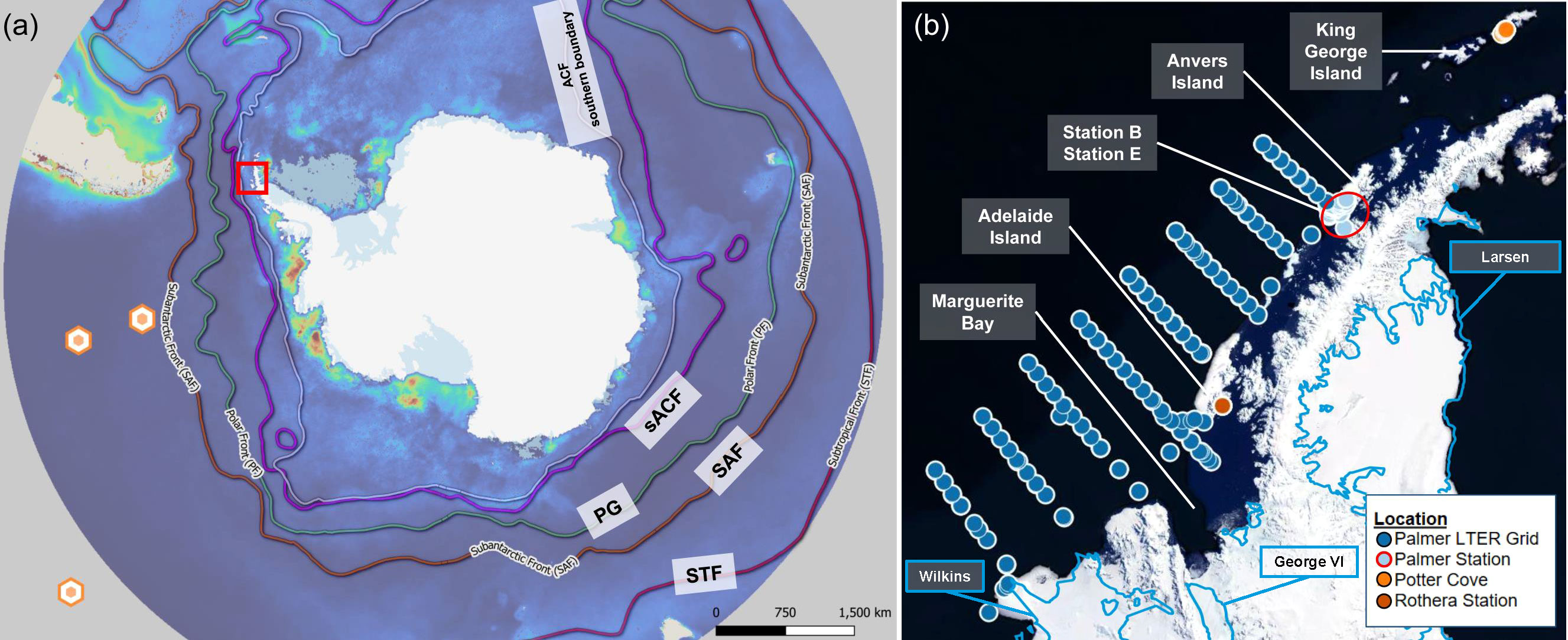
Figure 1 Area of interest. (A) Overview of Antarctica; orange points indicate synthetic blank sampling locations (i.e., regions assumed to have zero glacial meltwater) and the red box denotes the Western Antarctic Peninsula (WAP). The background is the MODIS chlorophyll-a concentration austral summer climatology (2002-2016); sACF, Southern Antarctic Circumpolar Current Front; PG, Polar Front; SAF, Subantarctic Front; STF, Subtropical Front. (B) The WAP and oxygen isotope field data sampling locations. Blue outlines indicate major ice shelves in the region.

In addition to water sample collection over the WAP shelf, the Palmer LTER program also samples quasi-weekly during austral summer from two nearshore sites near the Palmer Research Station on Anvers Island (Figure 1B). Station B, located at 64.7795°S/64.0725°W, is <1 km from shore and in waters of 75 m depth. Station E, located at 64.815°S/64.0405°W, is farther offshore and more directly exposed to the continental shelf and open ocean, with a water depth of 200 m. The start of each sampling season is subject to boat access due to severe weather conditions and sea ice presence, thus ranging from mid-October to late December. During austral winter, when boat operation ceases, the Palmer LTER program also samples seawater through an inlet at 5.8 m depth, located at 64.7738°S/64.0545°W. These nearshore stations are situated near the shallow marine-terminating Marr Ice Piedmont and other land-based ice masses (Meredith et al., 2021) (Figure 1B).

The combined field dataset also contains δ¹⁸O seawater samples from additional nearshore stations at Potter Cove and Maxwell Bay, located on King George Island (Figure 1B). Water samples were collected using 4.7 L Niskin bottles during water column profiling with a Sea-Bird SBE 19 CTD instrument (Meredith et al., 2018). Some field data from the Rothera Oceanographic and Biological Time Series (RaTS) were also included in the combined field dataset, albeit sparse due to a lack of matching MODIS-to-field data given its proximity to the shore of Adelaide Island (67.5700°S/68.2250°W) (Figure 1B). Water sampling here was also conducted in conjunction with CTD casts (Meredith et al., 2010). This expansive selection of study sites aligns with prior studies, such as the WAP research overviews provided by Ducklow et al. (2007) and Hendry et al. (2018), which often include islands and areas near the northern tip of the Peninsula.

2.2 Glacial meltwater fraction field data

From each of the sites mentioned, δ¹⁸O seawater samples at the surface were selected for this study. Surface is here defined as the shallowest sample depth in the water column within the top 5m, and δ¹⁸O is here measured in units of ‰. SSGM is derived based on mass balance calculations conducted in the aforementioned studies, and it is measured in units of freshwater % (Meredith et al., 2010; Meredith et al., 2017a; Meredith et al., 2018; Meredith et al., 2021). Each discrete δ¹⁸O sample is paired with its corresponding salinity values from CTD data. The mass balance calculation presumes each sample is composed of a simple mixture of three components – ocean water (ow), sea ice meltwater (sim), and meteoric water (met), with the latter term being the sum of precipitation and glacial meltwater:

$\begin{array}{ll}{F}_{sim}+F_{met}+F_{ow}=1& (1)\end{array}$

$\begin{array}{ll}{S}_{sim}·F_{sim}+S_{met}·F_{met}+S_{ow}·F_{ow}=S_{total}& (2)\end{array}$

$\begin{array}{ll}{\delta }^{18}{O}_{sim}·F_{sim}+ {\delta }^{18}{O}_{met}·F_{met}+ {\delta }^{18}{O}_{ow}·F_{ow}= {\delta }^{18}{O}_{total}& (3)\end{array}$

This system of equations is solved for F_sim, F_met, and F_ow, which are the respective fractions of the three components in each sample. S_sim, S_met, and S_ow are the salinity values for the end-member source components, while δ¹⁸O_sim, δ¹⁸O_met, δ¹⁸O_ow are the corresponding δ¹⁸O values. Endmember values are taken from the previous studies that generated our combined field dataset (Table 1); these data sources include Palmer LTER grid (Meredith et al., 2017a), Palmer Station on Anvers Island (Meredith et al., 2021), Potter Cove (Meredith et al., 2018), and Rothera Point on Adelaide Island (Meredith et al., 2010) as described above.

TABLE 1

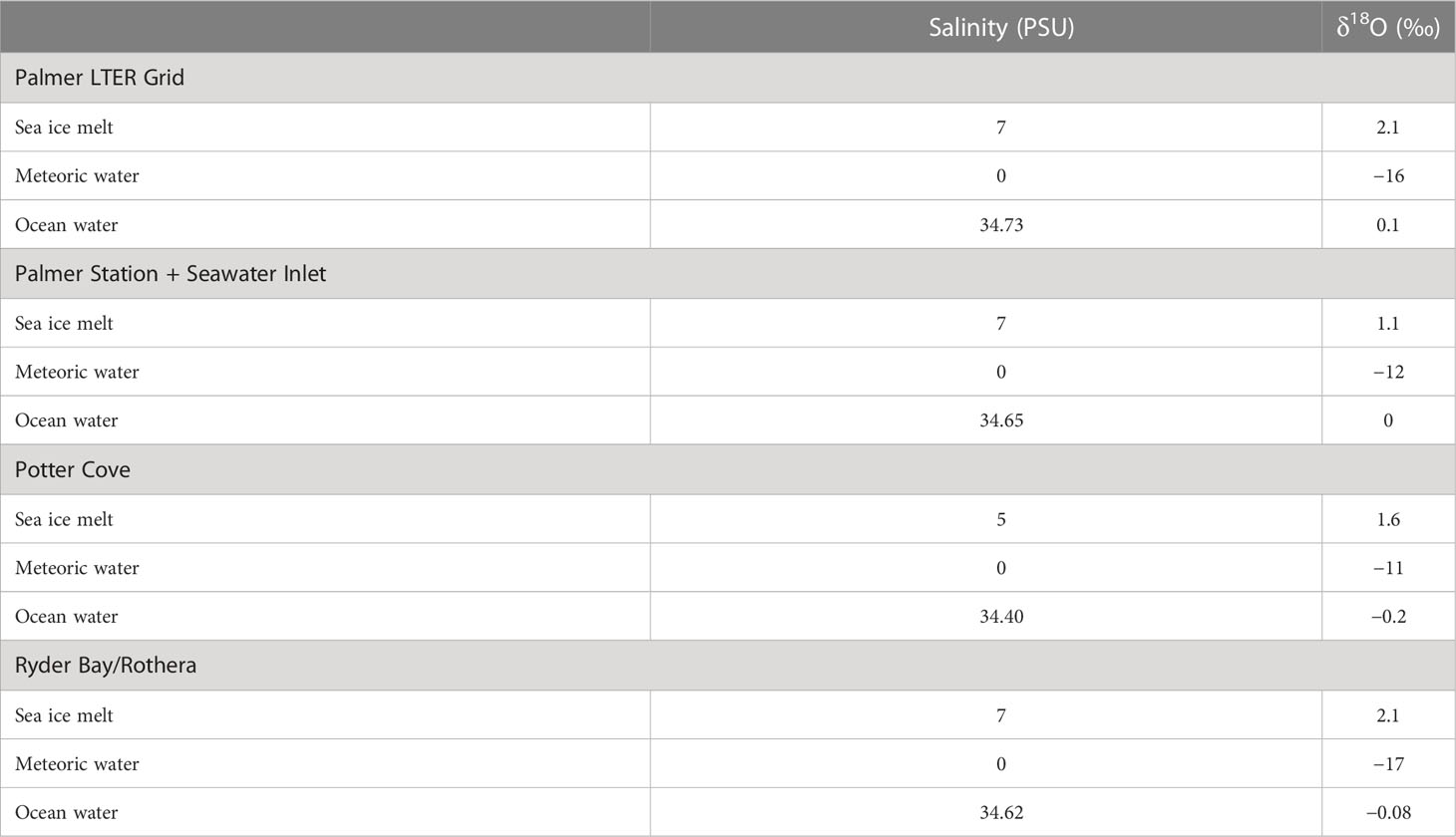
Table 1 End member values for mass balance calculations of meteoric water and sea ice meltwater fractions.

2.3 Spaceborne multispectral data

MODIS-Aqua Level 3 remote sensing reflectance data, R_rs(λ), for 10 spectral bands (i.e., 412, 443, 469, 488, 531, 547, 555, 645, 667, 678 nm where λ is light wavelength in vacuum) were acquired from the NASA Ocean Biology Distributed Active Archive Center (DOI: 10.5067/AQUA/MODIS/L3M/RRS/2018). Level 3 Ocean Color Standard Mapped Images at 4 km resolution were accessed via Google Earth Engine (GEE). An initial matchup dataset was compiled by iteratively reviewing all field data, and then matching each field data point with a set of corresponding MODIS pixel values that cover these field coordinates from the same date. Furthermore, the level 3 R_rs(λ) data already removes areas with sea ice, thus eliminating the potential of sea ice contamination in the overall dataset. This process produced a dataset where each field measurement of meteoric water fraction was matched with its ten corresponding MODIS R_rs band values. Out of the 86 matchups, 38 were from the Palmer LTER grid, 42 from the Palmer Station site, and 6 from Potter Cove or the Rothera Time Series. The low matchup availability is mostly due to cloud cover. This initial dataset also needs very low or zero glacial meltwater values for standard machine learning models to effectively detect a wide range of target values. Therefore, the initial dataset was also supplemented with synthetic “blank” meteoric water samples. For each date when a field-MODIS data point pair is found, a synthetic blank sample is also obtained at three locations on the outside of the Antarctic Circumpolar Current (ACC) (Figure 1A). They were sampled at 47.2382°S/99.1695°W, 54.3690°S/97.1654°W, and 35.5635°S/129.8333°W. For each “blank” sample, a value of 0% glacial meltwater fraction was assigned to the R_rs band values obtained for these pixels.

2.4 Data processing & model development

In this study, the MODIS R_rs(λ) band values are input variables while meteoric water fraction is the target variable. The input variables are the ten ocean color band values of R_rs(412), R_rs(443), R_rs(469), R_rs(488), R_rs(531), R_rs(547), R_rs(555), R_rs(645), R_rs(667), R_rs(678), and band math values for R_rs(555) + R_rs(667), and R_rs(667)/R_rs(488) per previous AOP models for retrieving glacial meltwater fraction (Pan et al., 2019). In order to model the data, we executed a three-step process involving: (1) algorithm selection, (2) hyperparameter optimization of the selected algorithm using train, validation and test subsets, and (3) final model training with the best hyperparameters on the complete dataset. For algorithm selection, we used a method of evaluating thirty-six different regression algorithms, including adaptive boosting, support vector machines, k-nearest neighbors, linear regression, gradient boosting, an individual decision tree and a random forest, among others (https://scikit-learn.org/stable/supervised_learning.html). The selected algorithm had to be reasonably interpretable, so algorithms like advanced neural networks were excluded. The primary goal of this preliminary step is to understand how different models would respond to the SSGM training dataset as well as their general performance without extensive model tuning, such as hyperparameter search.

After identifying the random forest algorithm as the best-performing in the initial evaluation, we conducted a hyperparameter search to fine-tune the following hyperparameters: n-estimator, which is the number of decision trees in a random forest; minimum-samples-leaf, which is the minimum number of samples that should be present in the leaf node after splitting a node; and minimum-samples-split, which is the minimum number of data points in any given node in order to split it.

Hyperparameter optimization is the process of iteratively tuning a learning algorithm’s hyperparameters in order to better fit training data. Overfitting is a common problem when utilizing this technique (Cawley and Talbot, 2010; Feurer and Hutter, 2019). To avoid overfitting, the dataset was split into training (80%), validation (10%) and test subsets (10%) (Figure 2). The training subset was used to train 10000 candidate models. The cross-validation accuracy score for each model was evaluated using the validation dataset. There are a number of search algorithms used in hyperparameter optimization – most commonly grid search, random search and Bayesian algorithms. A Tree-structured Parzen Estimator (TPE), which is a Bayesian technique, enables a more efficient search of the hyperparameter space than grid or random searches (Bergstra et al., 2011). This means new hyperparameters were selected iteratively based on the previous performance of those hyperparameters, as measured against the validation dataset. The best hyperparameters were 265 n-estimators, a minimum-samples-leaf of 1, and a minimum-samples-split of 8. The maximum depth of the random forest is not predetermined, and the decision trees’ nodes are expanded until all leaves contain less than the minimum-samples-split. At the completion of the hyperparameter search, a model was selected and evaluated against the test dataset. This means that the test dataset was used only once during the entire modeling process (Figure 2).

FIGURE 2

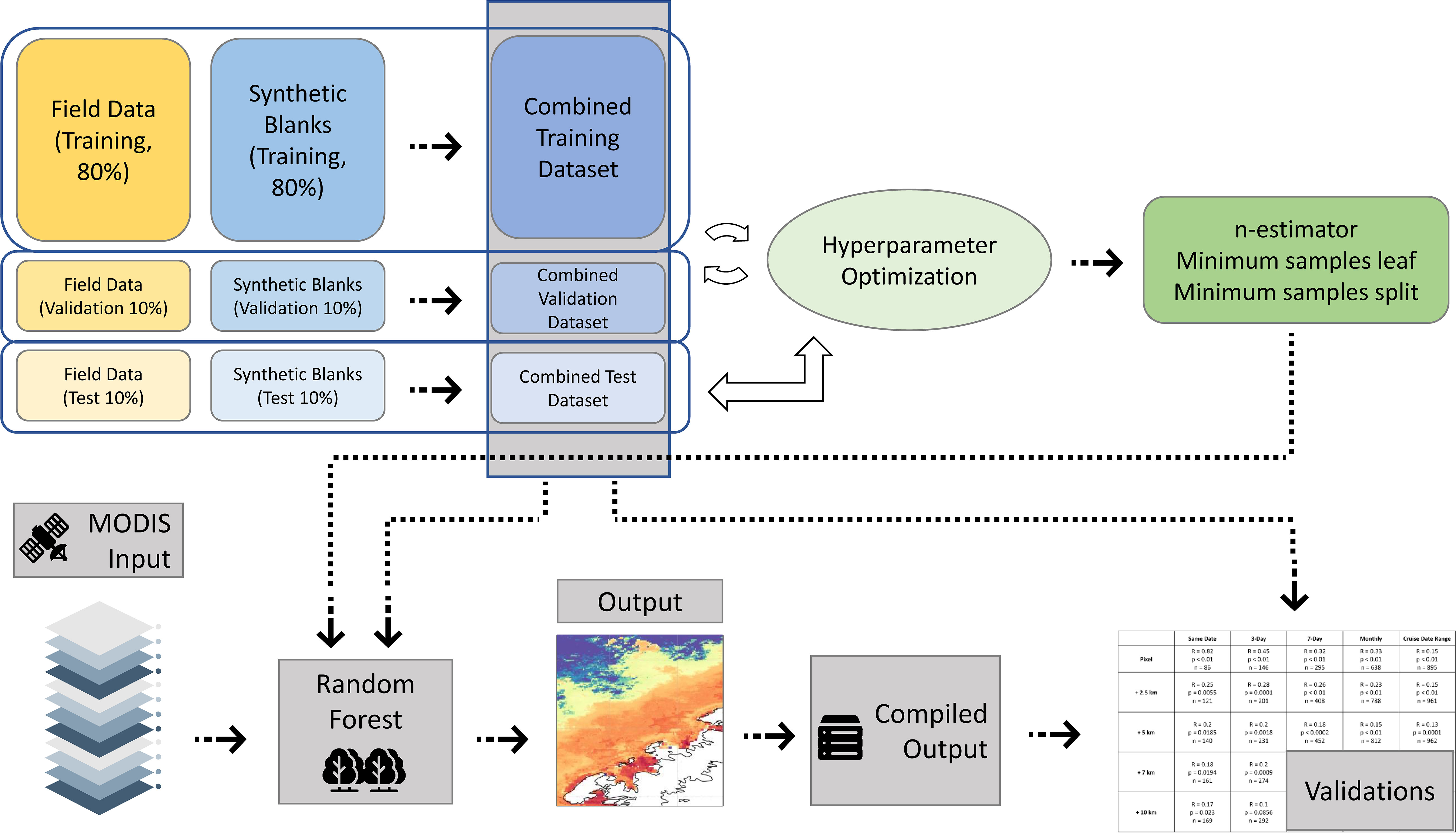
Figure 2 Model training and validation workflow implemented in this study.

The finalized model is trained using data and settings described earlier in this section – all available R_rs bands and band math as well as the random forest model hyperparameters determined from the TPE-based search process. The finalized model is deployed with geemap (Wu, 2020), a Python package for interactive mapping with GEE, using the native GEE random forest function. The MODIS-Aqua level 3 dataset was compiled in GEE using its NASA/OCEANDATA/MODIS-Aqua/L3SMI image collection (DOI: 10.5067/AQUA/MODIS/L3M/RRS/2018). Further model validation was conducted to assess the model’s robustness and to gain insights on its applicability to spatially and temporally averaged MODIS data (Figure 3). Spatially, each field data point is compared with the MODIS-based prediction that encompasses the field data coordinates (Figure 3 row 1, column 1), and then the field data point is also compared with spatially averaged MODIS-based predictions – by adding 2.5 km, 5 km, 7.5 km, and 10 km to each side of the pixel to create a new area of interest, and then averaging all predicted values that fall within the new target areas respectively (Figure 3 rows). Temporally, each field data point is compared with the MODIS-based prediction from the same date (Figure 3 row 1, column 1), and then the field data point is also compared with predicted values averaged over 3 days, 7 days, monthly, and date range covering the Palmer LTER cruises which varies annually (Figure 3 columns). These comparisons generate a matrix of 25 configurations of different spatial and temporal correlations between field data and predicted values (Figure 3). For each comparison configuration, we evaluated the Pearson’s correlation coefficient (r), p-value, sample size and a visualization of the correlations as scatter plots (Figure S1). Additional statistical measures were produced to evaluate the SSGM model by focusing on the correlation between the daily MODIS-based values and discrete field data (Figure 3 row 1, column 1). The loss of correlations between field data and spatiotemporally averaged predictions can provide some indications on SSGM’s spatial scale and residence time.

FIGURE 3

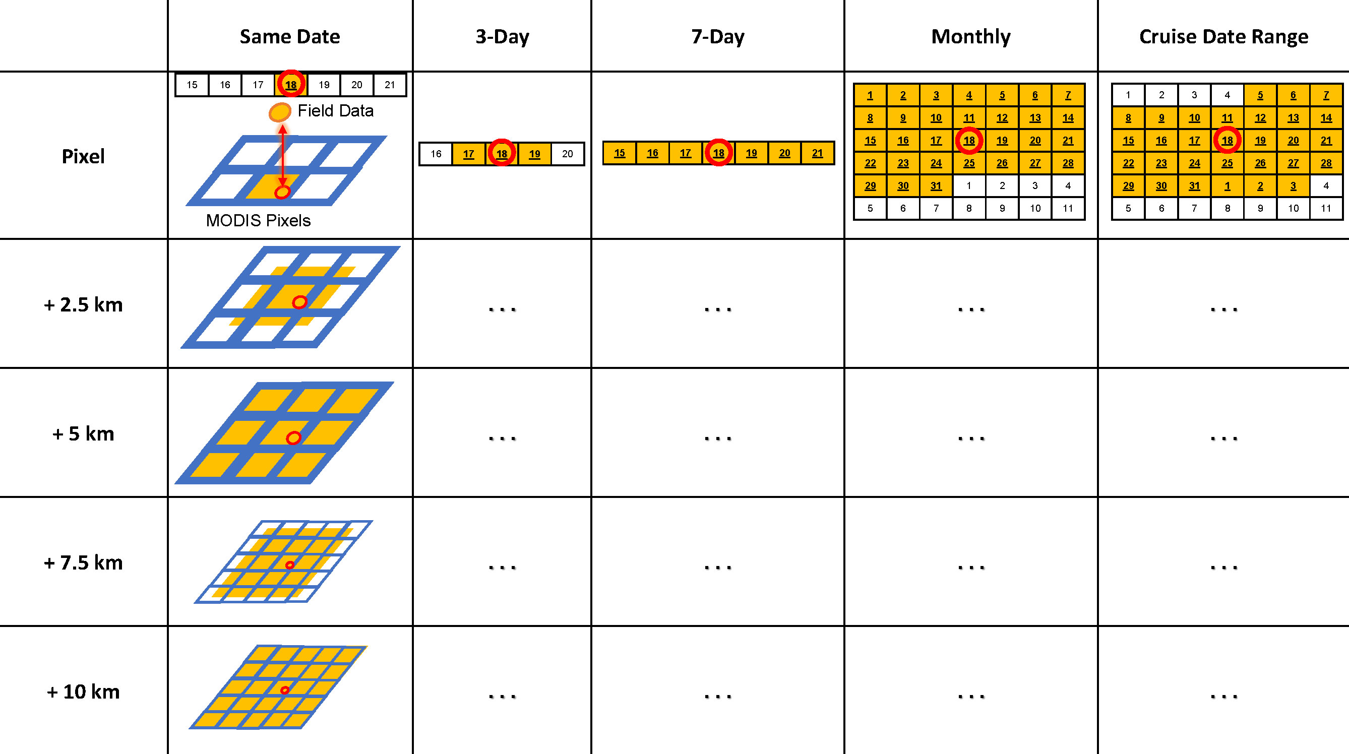
Figure 3 Conceptual diagram of the validation matrix in this study. In addition to comparing each field data point with its corresponding daily MODIS-based value (row 1, column 1), each field sample is also compared with spatially and temporally averaged MODIS-derived values.

2.5 PRISM airborne dataset

The final SSGM model was also applied to airborne imaging spectroscopy data from the NASA/JPL Portal Remote Imaging SpectroMeter (PRISM) (Mouroulis et al., 2014), collected as part of the O₂/N₂ Ratio and CO₂ Airborne Southern Ocean (ORCAS) campaign in January-February 2016 (Stephens et al., 2018), to further assess the model’s applicability across platforms. The goal was to demonstrate the spatial resolution advantages of such airborne datasets. PRISM flew on the NSF/NCAR Gulfstream-V aircraft at an approximate altitude of ~12.2 km providing water-leaving radiance and remote sensing reflectance from 350 to 1050 nm, approximately every 3 nm, with 10 m spatial resolution (https://prism.jpl.nasa.gov/dataportal/). Atmospheric correction was conducted using an Optimal Estimation formulation that simultaneously models surface and atmospheric reflectance contributions from statistical priors (Thompson et al., 2018; Thompson et al., 2019). The PRISM ORCAS data were pre-processed in ENVI^® to extract R_rs(λ) bands according to MODIS wavelengths and the images were exported to GEE as GeoTIFF files. Here, we assume that the PRISM bands near the targeted MODIS bands would perform similarly. The final SSGM model was applied to each airborne image to retrieve glacial meltwater fraction.

3 Results

3.1 SSGM model evaluation

When the predicted glacial meltwater fraction values and field data are compared during the development phase (Figure 2), we found the validation dataset had an r value of 0.878 and the test dataset had an r value of 0.885. The r values across both datasets are relatively high, and notably, these r values are relatively consistent indicating the hyperparameter search did not cause the model to overfit against the validation data. This evaluation confirms the model’s overall performance, so all development datasets were combined to produce the final model for this study. After the final version of the model is applied to MODIS-Aqua data, we found relatively high r value when field data are compared to predictions based on matching pixel values from the same dates (r = 0.82, p < 0.01). However, the correlation decreases as the MODIS-based predictions are averaged over longer time periods (Table 2, columns). The decrease in correlation is even more pronounced when the predicted values are averaged over larger areas (Table 2, rows). Figure S1 presents a visualization of these correlations as scatter plots.

TABLE 2

Table 2 Validation matrix illustrating the comparison between field data and MODIS-derived values.

To further evaluate the model performance, several statistical measures were calculated to describe the regression function between field data and daily MODIS-derived SSGM values (without spatial or temporal averaging, Figure S1 row 1, column 1). These measures are commonly used for evaluation in biogeochemical modeling and bio-optical studies (Brewin et al., 2015; Seegers et al., 2018) (Figure 4; Table S.1). We found that the residual differences between MODIS-derived SSGM and field data have a symmetric probability distribution around a median of 0.04%. The median ratio (MdR) and median bias (MdB, in units of predicted variable) measures are produced to characterize systematic deviations, while the median absolute percentage difference (MdAPD) and root mean square error (RMSE, in units of predicted variable) are used to characterize random deviations between modeled SSGM values and field data. A model that provides the best overall fit to in-situ data should have MdR close to 1 and low values of MdB, MdAPD and RMSE. We found MdR = 0.990, while MdB = −0.040, MdAPD = 6.375%, and RMSE = 0.463. Moreover, errors in remote sensing and bio-optical models are also often reported by statistical indicators calculated based on linear regression between in-situ and predicted values. Here, we calculated the statistical measures based on Model II least-squares fit (Ricker, 1973), because both satellite- and δ¹⁸O-derived values presented in Figure 4 are collected from an uncontrolled environment, subject to error, and are dependent on the actual SSGM fractions in the field. The slope of the line is determined by calculating the geometric mean of the slopes from the regression of Y-on-X and X-on-Y (Sokal and Rohlf, 1995). The best-fit coefficients of the regression function and correlation coefficient reveal the degree to which the predicted values agree with measured values over the entire dynamic range. For instance, deviations from 1 for the slope and deviations from 0 for the intercept (A) of the fitted regression reveal the variation in the bias of SSGM predictions relative to the field data across its full range (Table S.1). These measures are further evaluated when our analysis considers outliers. The outliers were selected based on a Bland-Altmann plot (Figure S2) and they are defined as data points where the predicted SSGM value is beyond ±2 standard deviations from the mean of residuals between predicted and observed values.

FIGURE 4

Figure 4 Scatter plot of field data and predicted glacial meltwater values. The dashed line depicts the 1:1 reference line.

3.2 SSGM model analysis

Further model diagnostics were conducted to evaluate the model’s performance and to better understand the relationship between the R_rs(λ) values and predicted SSGM fraction values. In Figure 5, the model’s input variables are ranked by the amount of variance that they explain. The top variable, R_rs(667)/R_rs(488), explains 82.96% of total variance. The following two variables – R_rs(443) and R_rs(412) – explain an additional 7.35% cumulatively. Therefore, the top three input variables explain a total of 90.31% of the variance. The remaining input variables explain 9.69% of the total variance (Figure 5).

FIGURE 5

Figure 5 The ranking of R_rs(λ) variables based on the final model to predict sea surface glacial meltwater fraction. The bar graph represents the percentage of variance in the model that is explained by each R_rs(λ) variable; the values on the right present the cumulative percentage of explained variance in the model.

Notably, we intentionally introduce R_rs bands that were designed for terrestrial and atmospheric applications – in particular, Band 1 centered around 645 nm, Band 3 centered around 469 nm, and Band 4 centered around 555 nm. The results demonstrate the model’s ability to distinguish valid information (i.e., various R_rs bands designed for ocean observation were selected as top input variables and they can explain 90.31% of the model’s total variance). These results also highlight the model’s robustness to provide valuable insights instead of merely over-fitting to the target variable with all available input data indiscriminately.

The response of each input variable is also examined in more detail. We use individual conditional expectation plots to present the responses of decision trees within the random forest model to changes in each input variable (Molnar, 2020). In each panel of Figure 6, the blue lines represent how individual decision trees predicted SSGM fraction values change according to the input R_rs(λ) values, while the red line represents the average prediction of these decision trees (Figure 6). Within the top five input variables (Figure 5), predicted SSGM values increase abruptly when R_rs(667)/R_rs(488) is over 0.05 meanwhile a more gradual decrease in SSGM is observed for input variables R_rs(443), R_rs(412) and R_rs(469) when they increase from 0.005 sr^-1 to 0.01 sr^-1. Additionally, a gradual increase in SSGM is observed when R_rs(645) increases from 0.00025 sr^-1 to 0.0005 sr^-1. In contrast, the model exhibits minimal change in predicted SSGM values according to changes in some input variables, such as R_rs(678), R_rs(667), and R_rs(555) (Figure 6).

FIGURE 6

Figure 6 Individual conditional expectation plots display one line per decision tree in the final random forest model that shows how the changes in R_rs(λ) values impact the predictions of sea surface glacial meltwater fraction.

3.3 MODIS-Aqua data application

The final model is applied to MODIS-Aqua data to provide visualizations of SSGM. Figure 7 represents the December, January, and February monthly climatology between 2010 and 2020. The austral summer months coincide with most of the sampling time periods of our field data. SSGM is most abundant along the coast and extends across the WAP continental shelf into the open Southern Ocean. High SSGM is also observed around islands and nearshore locations around outlets of glacial fjords. Notably, some high SSGM is also observed near the Larsen C Ice Shelf on the eastern side of the Peninsula. Overall, there appears to be more glacial meltwater on the southern end of the WAP, particularly in Marguerite Bay and near the Wordie Ice Shelf (Figures 7A, D, G). The SSGM monthly climatology is also compared to surface chl-a concentration and sea surface temperature (SST) from the same time periods. High SSGM values appear to coincide with chl-a concentrations, but there is a distinct difference in their spatial patterns over the entire WAP (Figures 7B, E, H). Similarly, some nearshore high SSGM is found to coincide with low SST, especially in Marguerite Bay and between Adelaide Island and Lavoisier Island (Figures 7C, F, I).

FIGURE 7

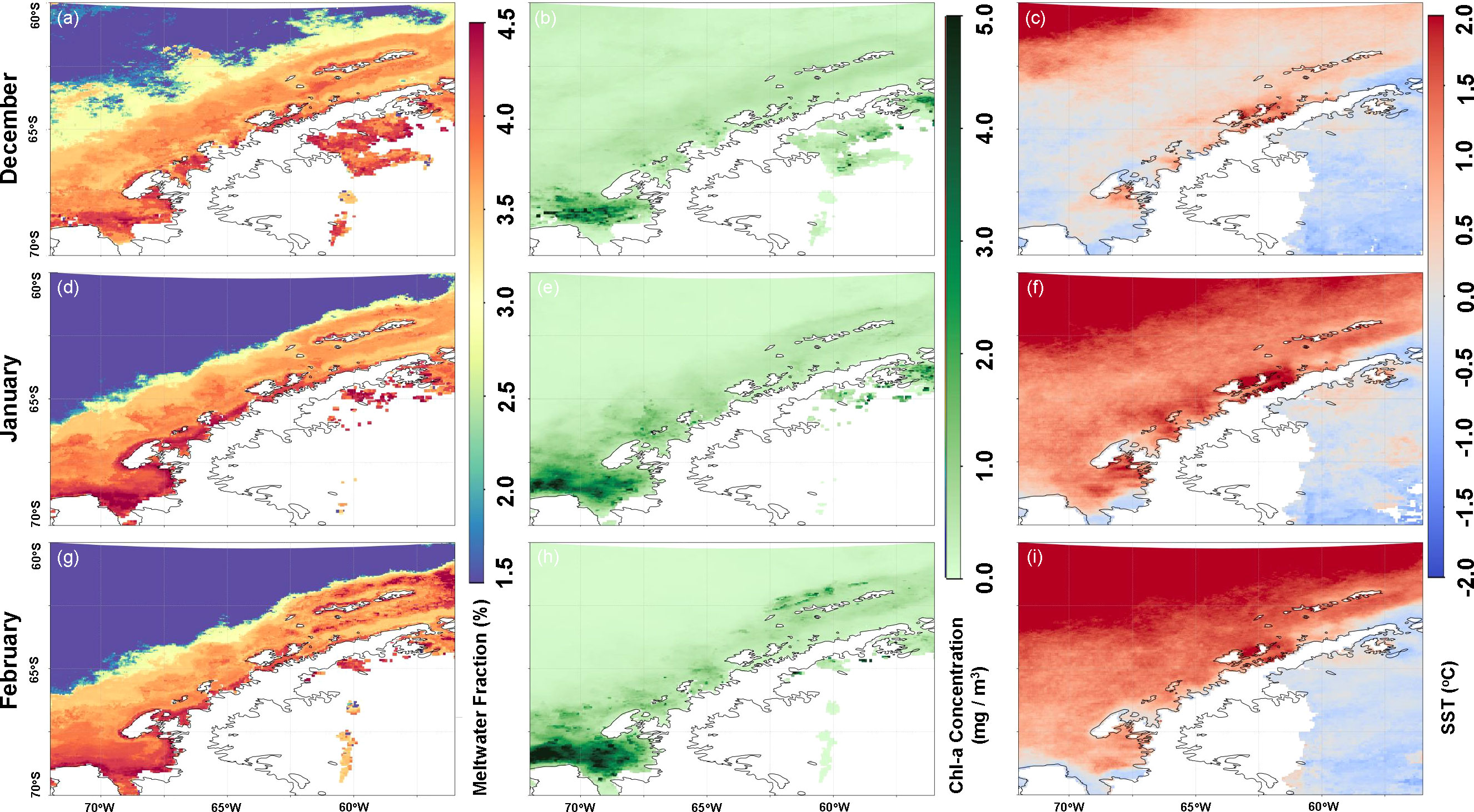
Figure 7 Monthly climatology of the Austral summer months from 2010 to 2020: (A, D, G) sea surface glacial meltwater, (B, E, H) chlorophyll-a concentration, and (C, F, I) sea surface temperature derived from MODIS-Aqua.

3.4 PRISM airborne data application

The SSGM model was also applied to PRISM airborne ocean color data to assess the model’s applicability across remote sensing platforms. PRISM scene prm20160125t181722 is presented in Figure 8, collected NW of Anvers Island. The entire scene has an average of 3.94% SSGM fraction. A few icebergs < 1km in size can be found in the middle of the scene (Figure 8C) and, in contrast, the maximum SSGM fraction reaches 6.49% in the vicinity of the icebergs (Figure 8D). Overall, the SSGM derived from airborne data shows consistent spatial distribution as the MODIS-based values. In particular, a distinct front can be observed in both datasets immediately south of 64 °S (Figure 8A). This consistency in the SSGM spatial distributions derived from different remote sensing platforms illustrates the potential for applying the model to other ocean color datasets beyond MODIS. Moreover, the airborne data demonstrates its significant advantage of having finer spatial resolution; for example, meltwater from the icebergs cannot be observed in the spatially coarse MODIS-based SSGM data, but it can be detected using the airborne data. Notably, a trail of bergy bits (Dowdeswell and Forsberg, 1992) from the icebergs can be clearly seen in both enhanced RGB image and SSGM data from PRISM (Figures 8C, D). There are also some discrepancies between the PRISM- and MODIS-derived SSGM values. The differences are likely due to the different processing methods of the remote sensing data from the two different platforms (Material & Methods 2.3, 2.4, and 2.5), The discrepancies are also likely resulted from their temporal difference between the times of data acquisition, which is several hours apart.

FIGURE 8

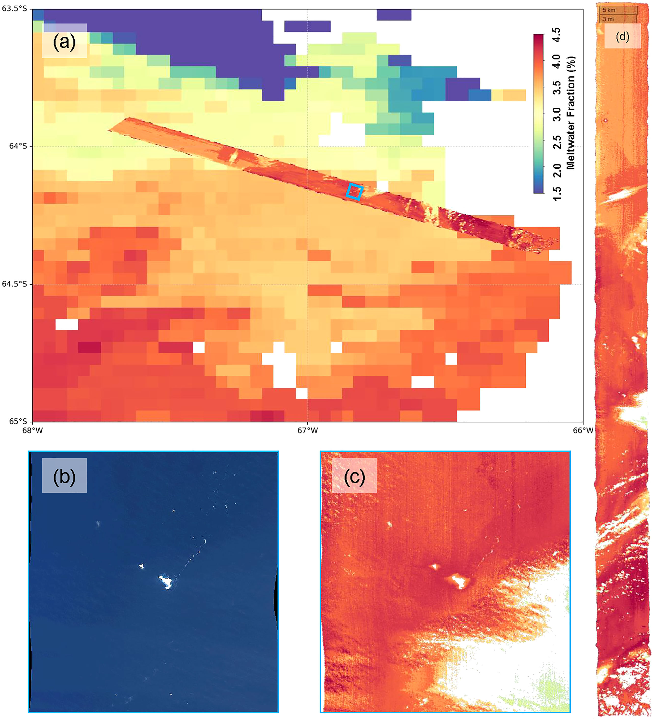
Figure 8 (A) PRISM airborne data (prm20160125t181722) overlaying MODIS-derived surface glacial meltwater fraction from January 25^th, 2016. (B) Enhanced RGB image zoom of the blue square in panel a, depicting icebergs and a trail of bergy bits. (C) Derived glacial meltwater fraction in the same region as panel (B). (D) A detailed overview of scene prm20160125t181722.

4 Discussion

4.1 SSGM model assessment

The final model is applied to MODIS-based predictions over different spatial and temporal scales. A notable feature is the formation of a “threshold” that is parallel to the x-axes when predicted SSGM values are averaged over extended spatial and temporal scales (Figure S1). This horizontal cluster of data points indicates that it is unsuitable to compare a single field data point with averaged SSGM prediction over extended space and time periods. Because of this, future use of this model should only involve other datasets that are on a similar spatial and temporal scale as the SSGM data product. For an instance, daily 1 km resolution SSGM product should not be directly merged with 8-day 4 km resolution chl-a product; a SSGM composite should be created first before merging the datasets. The rapid decrease in r values across the comparison matrix (Table 2) also represents a potential indication of residence time and spatial extent of SSGM features. While this speculation can only be confirmed with additional studies beyond the scope of this project, it still offers some information on the spatial and temporal requirements for future field campaigns and remote sensing missions to effectively resolve SSGM features.

When the final model’s predictions are compared with the field data, most predicted values appear to slightly over-estimate SSGM, but within an acceptable range (Figure 4). In contrast, outliers appear to significantly underestimate SSGM (except for one sample, Figure S2). Statistical measures shown in Table S.1 have been carried out to analyze the dataset, with and without the outliers, and both analyses show relatively consistent results (Table S.1; Figure S4). The slope of the regression line between modeled and in-situ values decreased from 0.931 to 0.771 after outliers were removed. This indicates that the model exhibits some remaining patterns in bias over the entire range of data, as seen in Figure S2 and Figure S4. They may be related to potentially higher measurement uncertainties in some data ranges (e.g., low values of SSGM) or result from uncertainties in spatio-temporal matching of satellite and in-situ measurements. We note, however, that apart from these regression line metrics, all other statistical indicators in Table S.1 of aggregate model bias and random error improved following the removal of these outliers, and overall support the potential utility of this preliminary model developed based on a relatively limited training dataset. Additional observations, particularly in the lower and upper ranges of SSGM, are needed to better assess model uncertainties and improve model performance across the entire SSGM range.

4.2 Additional SSGM validation

4.2.1 The physical basis for SSGM remote detection

Previous studies conducted in Greenland fjords have demonstrated the effectiveness of leveraging multispectral ocean color datasets (such as MODIS) to retrieve suspended sediment concentrations in Arctic polar waters (Chu et al., 2010; Hudson et al., 2014). The suspended sediments described in these studies are associated with glacial meltwater discharge and could reach > 600 mg/l on average – effectively becoming a proxy for ice-sheet runoff. In contrast, the glacial meltwater injection at the WAP is less intense and therefore it often lacks the prominent surface sediment plumes often found in Greenland and the broader Arctic region (Pan et al., 2019). However, while there were no glacial sediment plumes by visual inspection, field studies conducted in a WAP fjord (Andvord Bay) found significantly higher values of seawater inherent optical properties near the glacial-marine interface – where particulate backscattering coefficient at 442 nm reached a maximum of 0.01 m^-1 and particulate beam attenuation coefficient at 660 nm reached a maximum of 2.21 m^-1 in the inner basin of the fjord (Pan et al., 2019). Moreover, these optical signals near the glaciers in Andvord Bay are persistent features – field work conducted in the latter part of the last century also detected high beam attenuation coefficient values near the glacial front, with a maximum of ~2 m^-1 (Domack and Williams, 1990). These prior studies offer some indications that the presence of SSGM is intrinsically associated with fine suspended glacial sediments.

If SSGM can be quantified as fine particle plumes, then it is expected that SSGM would share some attributes with surface plume features where they would closely interact with other physical oceanographic features, such as currents and eddies. For context, there are some prominent features in the WAP region. The dominant feature offshore is the Antarctic Circumpolar Current (ACC) flows along the WAP continental shelf (Martinson et al., 2008). In addition, there is a less intense coastal current (Antarctic Peninsula Coastal Current, APCC) which flows southward along the western shore of Adelaide Island and Alexander Island (Stein, 1992; Moffat et al., 2008; Savidge and Amft, 2009; Meredith et al., 2010). The coastal current, specifically, exhibits seasonal variability and is thought to be partially driven by buoyancy-forced fresh meltwater supply (Beardsley et al., 2004; Savidge and Amft, 2009).

Other mesoscale physical oceanographic features, such as eddies and loops, can also significantly impact SSGM distribution in space and over time. A prior study using high-frequency radar network deployed near Anvers Island (at Palmer Deep canyon) found surface particle assemblage residence time was between 1 and 3.5 days with a mean of 2 days and a maximum of 5 days (Kohut et al., 2018). Similarly, a previous study using the Regional Ocean Modeling System (ROMS, adapted for the WAP region) found an overall median residence time of 4.1 ± 3.3 days for simulated neutrally buoyant particles released at the surface (Hudson et al., 2021). More specifically, the ROMS study found the residence time ranged between 1.5 ± 0.7 and 2.3 ± 0.3 days over the WAP continental shelf, and it ranged between 2 ± 1.2 days and 7.1 ± 3 days in the coastal waters near Anvers Island (Hudson et al., 2021). These residence times are similar to the time frames reflected in our MODIS-field-data validation matrix (Table 2; Figure S1). We observed a clear lack of correlation that begins to form when > 3 days of MODIS data are averaged and matched with field data points (Table 2, Figure S1). The discrete SSGM field data should not be compared with temporally averaged MODIS-based values, indicating the importance of having consistent time frames when SSGM modeled values are assembled with other datasets in future studies. More importantly, we speculate that the decrease in correlation across the matrix potentially alludes to the residence time of SSGM as it interacts with the WAP’s physical oceanography. This provides additional insights on the appropriate temporal resolution that is needed to support future field campaigns and remote sensing missions that have the potential to study glacial meltwater in the WAP (Cawse-Nicholson et al., 2021).

4.2.2 Remote sensing and optics of SSGM

The SSGM model appears to track fine particle assemblage associated with glacial meltwater, allowing detection of SSGM from remote sensing platforms. The optics of glacial meltwater is expected to resemble that of fine suspended sediments in a water column. Sravanthi et al. (2013) conducted a comprehensive review of R_rs at various wavelengths and their linear relationships with suspended particulate mass concentration (SPM) in Kerala, coastal ocean of the Arabian Sea. They also examined several R_rs(λ) band math variables, particularly R_rs(555) + R_rs(620) and R_rs(620)/R_rs(490) which showed high correlations with SPM. This information resulted in a multivariant linear model for deriving SPM (mg/l) based on R_rs(λ):

$\begin{array}{ll}SPM=14.93*\{[{\text{R}}_{\text{rs}}(555)+{\text{R}}_{\text{rs}}(620)]+{[\frac{R_{rs}(620)}{R_{rs}(490)}]}^2\}+ 8.22& (4)\end{array}$

Later, Pan et al. (2019) modified this model and applied it to the polar region for quantifying glacial meltwater in a WAP fjord, given the high optical signal found near the glacial-marine interface (Pan et al., 2019):

$\begin{array}{ll}GM=\beta + {\alpha }_1[\text{R}(555)+R(625)]+{\alpha }_2{[\frac{R(625)}{R(490)}]}^2 & (5)\end{array}$

where GM is glacial meltwater fraction based on in-situ δ¹⁸O data, α and β are constant coefficients, and R(λ) is defined as the ratio between upwelling radiance and downwelling planar irradiance at discreet depths. Although these previous studies were conducted using in-situ radiometers and offered different wavelengths from MODIS bands, we have adapted these methods for this study and obtained similar results. For instance, R_rs(667)/R_rs(488) accounts for over 80% of the variance within our SSGM model (Figure 5), and therefore predicted SSGM values are the most responsive to changes in this variable (Figure 6). Detailed laboratory-based studies of pure glacial meltwater samples are required to elucidate the inherent optical properties and size and chemical composition of these fine glacial particles beyond the scope of this study. These future laboratory-based measurements are needed to complement the hyperspectral nature of the next-generation ocean color satellite missions.

Moreover, the predicted SSGM values appear to coincide with high chl-a concentrations, but they have distinctly different spatial distributions (Figure 7). This indicates our SSGM model is not merely capturing phytoplankton’s optical signal, which is a major optical constituent in the WAP. This notion is further confirmed by the ranking of variable importance (Figure 5) and individual conditional expectation plots (Figure 6) where predicted SSGM does not appear to be significantly correlated with bands commonly associated with chl-a detection. These insights and relatively consistent results across multiple studies indicate the SSGM model has likely captured significant key aspects of the underlying optics of glacial meltwater.

4.3 Assumptions and uncertainties

There are inevitably some assumptions and uncertainties associated with the SSGM model. One area of uncertainty is the quantity of the final (combined) training dataset (n = 204, including synthetic blanks). While this dataset is relatively small in comparison to machine learning projects in industry, the range of field data values in the dataset helps train a representative and robust model. Within the dataset, high meteoric water content was captured near Potter Cove. Many of these surface meteoric water samples were comprised of almost entirely glacial meltwater associated with heavy sediment discharge at this site (Meredith et al., 2018). These high meteoric water contents during the growing season are also consistent with the low salinity and high turbidity observed in the nearby Admiralty Bay (Osińska et al., 2023). Low SSGM content was introduced to the dataset via synthetic blanks that were generated outside of the ACC in the Southern Pacific open ocean (Figure 1). This gradient of SSGM captures the full range of meltwater content and their corresponding remote sensing reflectance properties. Moreover, the training dataset in this study is one of the most comprehensive δ¹⁸O data compilation for the WAP region, including four long-term time series at different locations (Material and Methods).

There are also assumptions and uncertainties associated with the field dataset itself. Because the meteoric water content was computed through mass balance calculations (Material and Methods), these values are sensitive to the selection of end member values (i.e., pure glacial and sea ice meltwater δ¹⁸O and salinities). To mitigate these uncertainties, a consistent and rigorous methodology was used during these field studies to select end members that were locally or regionally representative (Meredith et al., 2017b). In addition, the meteoric water variable is comprised of precipitation and glacial meltwater (Material and Methods). While the current state of this method cannot partition these two components directly, δ¹⁸O sampling remains one of the most cost-effective and accessible methods for estimating meltwater content and it can be collected on most oceanographic and community science cruises (Cusick et al., 2020). Moreover, the meteoric water variable represents an upper limit of glacial meltwater estimation, which is still useful for obtaining insights on its surface distribution over space and in time.

Additionally, the “synthetic blanks” in this study (Material and Methods) were selected outside of the ACC, therefore their meteoric water content likely include no glacial meltwater but various amounts of precipitation. Since these blank samples have significantly lower optical signal in comparison to the in-situ data collected at the WAP (Figure S3), by setting the synthetic blanks as 0% SSGM, we have likely trained the model to neglect the effect of precipitation on SSGM predictions. SSGM prediction also appears to be only weakly sensitive to the selection of blank SSGM data (Figure S3). This assumption can be verified to some degree when daily precipitation data is compared with in-situ meteoric water fractions around Anvers Island (Figure S4). Precipitation data retrieved between 1989 and 2019 shows high meteoric water content is associated with low precipitation (Figure S4A). Furthermore, the majority of this dataset is associated with no precipitation. Out of 410 data points, 219 are associated with 0 mm of rainfall, 361 are associated with 0 cm of snow precipitation, and 282 are associated with no accumulation by snow stake (Figure S4A). In addition, the anomalous values that fall away from the validation line in Figure 4 have been identified as outliers, and these values are also associated with low precipitation (Figure S4B, S4C). Hence any predictions that deviate from in-situ data is likely not due to excess precipitation interfering with glacial meltwater signals in δ¹⁸O samples. Due to the complex relationship between precipitation and the δ¹⁸O measurement, such as land-accumulated snow melt discharging into the ocean during summer or any precipitation events that might have occurred shortly before in-situ sampling, data presented in Figure S4 do not definitively decouple glacial meltwater from precipitation. However, these additional results indicate that δ¹⁸O has value as an effective in-situ measurement for estimating glacial meltwater in the WAP, and for training models for predicting SSGM. In the future, additional cost-effective tracers should be explored to enable partitioning of meteoric water content.

4.4 SSGM model applications

The SSGM model has provided important results with broader implications. For instance, the variable importance ranking shows the model is primarily dependent on a few key R_rs wavelengths, indicating these wavelengths are important to capturing the underlying optical characteristics of SSGM (Figure 5), though to a lesser extent, additional bands can also contribute to an increase in overall prediction power of the model, illustrating the merit of utilizing hyperspectral airborne ocean color data for future SSGM model development. Hyperspectral airborne data have several other advantages – such as its high spatial and temporal resolutions which reveal detailed features of SSGM distribution that cannot be resolved with MODIS data (Figure 8), as well as its increased spectral sampling that could provide additional spectral features not seen in multispectral data that can further tease out SSGM from other optical constituents. These results highlight the benefit of supplementing existing multispectral spaceborne datasets with hyperspectral airborne data in order to achieve better detection and monitoring of SSGM. Moreover, the application of this model on PRISM imagery indicates the applicability for other ocean color data products as well; in general, the model can generate SSGM results if the input R_rs data are at or near the MODIS bands (Figure 5) and are processed with consistent techniques used to produce MODIS Level 3 data products. Furthermore, the applicability of this SSGM model to both spaceborne and airborne datasets alludes to the possibility of sampling SSGM via Unmanned Aerial Vehicles (UAVs) (Pina and Vieira, 2022). Imaging instruments can be coupled with UAVs to achieve greater sampling frequency at a finer spatial resolution, while also being less susceptible to limitations of cloud cover, thus greatly complementing existing remote sensing platforms (Li et al., 2023). The potential of leveraging commercial UAV products to conduct sea surface imaging has been demonstrated by Wójcik-Długoborska et al. (2022) to study glacial suspended sediment plumes in the WAP.

Although this study demonstrates a new method for quantifying SSGM and its applicability across multiple remote sensing platforms, we stress that this is the first data product for quantifying SSGM remotely. While the SSGM predictions are validated with one of the most comprehensive in-situ δ¹⁸O datasets compiled for the WAP, there were no concurrent in-situ optical measurements; accordingly, our method takes an applied approach to correlate ocean color signals with field SSGM measurements. For the development of a first-generation model, we chose this applied approach for rapid implementation, so the results can be utilized by a wide range of end users for future projects. Additional laboratory studies are needed to understand the inherent and apparent optical properties of pure and diluted glacial meltwater.

The ability to monitor SSGM is directly relevant to understanding ecological dynamics that are being impacted by accelerating change along the WAP. The presence of SSGM is also found to coincide in regions of high chl-a concentrations. For example, phytoplankton abundance is found to be significantly correlated with glacial meltwater over the WAP shelf. This relationship extends >100km offshore and is persistent across years (Dierssen et al., 2002). The same dynamics between glacial meltwater and phytoplankton were also observed in a WAP fjord (Pan et al., 2020). In this study, we found similar spatial distributions between chl-a concentrations and SSGM but with clear distinctions between the two (Figure 7), consistent with prior studies. These results have important implications for polar ecosystem research. Remote sensing studies of the WAP ecosystem have primarily relied on measurements of chl-a, SST, sea ice properties, and salinity (IOCCG, 2015). However, in recent years, glacial meltwater has been identified as an additional environmental variable that is important to the ecosystem in the WAP and broader polar regions (Dierssen et al., 2002; Arrigo et al., 2017; Meire et al., 2017; Pan et al., 2020). Freshwater addition experiments in Potter Cove found that a gradual decrease in salinity can shift phytoplankton communities dominated by large centric diatoms to small pennate diatoms, suggesting a phytoplankton response to low salinity is species-specific (Hernando et al., 2015). Similar results have also been found in the field over the WAP shelf where cryptophyte abundance was observed to coincide with relatively low salinity waters (S ≤ ~33.6 PSU) (Moline et al., 2004). In addition, other studies found that glacial meltwater’s impact on phytoplankton communities is likely beyond changes in salinity. In WAP fjords, glacial meltwater is also a pathway for delivering macro- and micro-nutrients to the surface. Sporadic but prolonged katabatic wind events bring up deep nitrate-rich water which is propagated along the surface with SSGM from the ice-ocean interface (Ekern, 2017; Pan et al., 2020). Dissolved iron is supplied to the surface via a similar mechanism, but it can also directly enter the ambient water column via sub-glacial and sub-marine melting (Sherrell et al., 2018; Forsch et al., 2021). These results indicate that glacial meltwater plays an important role near the ice-ocean boundary, and SSGM export from fjords likely serves as an important nutrient source for the broader WAP ecosystem (Forsch et al., 2021). In short, detection of SSGM from remote sensing can provide a new proxy for monitoring the physical environment, ecosystem, and their variabilities in the WAP.

5 Conclusions

In this study, we present a data product for remotely quantifying SSGM in the WAP. The model can retrieve SSGM from ocean color datasets and is applicable across multiple remote sensing platforms. The model’s robustness is also assessed with one of the most comprehensive in-situ δ¹⁸O dataset complied for the WAP region. However, this model is not intended to be a definitive method for SSGM monitoring, but rather as an evolving model that will be frequently updated as more in-situ data, and data of other forms, becomes available in the future. We want to emphasize the need for persistent long-term in-situ δ¹⁸O sampling in the WAP region to ensure the future success of this model. Future model development can be aided by additional δ¹⁸O data and the inclusion of other techniques to partition SSGM.

Remote detection and monitoring of glacial meltwater present an important opportunity for understanding polar ecology and its physical environment. Given the complex dynamics amongst glacial meltwater, sea surface salinity, SST, nutrient availability and phytoplankton community abundance and composition, additional methods for monitoring and quantifying SSGM becomes necessary in order to achieve a better understanding of glacial meltwater’s impact on the WAP ecosystem. The potential of this SSGM model has important implications for studying the WAP ecosystem dynamics and the regional biogeochemistry.

Data availability statement

The raw data supporting the conclusions of this article will be made available by the authors, without undue reservation.

Author contributions

BP: Conceptualization, data curation, formal analysis, investigation, methodology, project administration, software, validation, visualization, writing - original draft, writing - review & editing; MG: Conceptualization, formal analysis, funding acquisition, methodology, project administration, resources, supervision, validation, writing - original draft, writing - review & editing; MM: Data curation, formal analysis, investigation, methodology, resources, validation, writing - original draft, writing - review & editing; RR: Conceptualization, formal analysis, methodology, validation, writing - review & editing; OS: Data curation, resources, validation, writing - review & editing; AO: Methodology, validation, writing - review & editing. All authors contributed to the article and approved the submitted version.

Funding

This research was carried out at the Jet Propulsion Laboratory, California Institute of Technology, under a contract with the National Aeronautics and Space Administration and Oak Ridge Associated Universities. The research was also partly supported through the FjordPhyto citizen science project (NASA 80NSSC21K0856). The views and conclusions contained in this document are those of the authors and should not be interpreted as representing the official policies, either expressed or implied, of NASA or the U.S. Government. The U.S. Government is authorized to reproduce and distribute reprints for Government purposes notwithstanding any copyright notation herein.

Acknowledgments

The authors would like to thank Mr. John W. Chapman and Mr. Winston Olson-Duvall at the Jet Propulsion Laboratory for supporting the preprocessing of the PRISM data. We would also like to thank the resources made available by the Google Earth Engine and Dr. Qiusheng Wu for his contribution to the Google Earth Engine community which made this project possible. The authors also want to thank the principal investigators and participants of the Palmer LTER Program (NSF 1440435), the Potter Cove sampling program, the Rothera Oceanographic and Biological Time Series, and the FjordPhyto citizen science project (NASA 80NSSC21K0856). Ms. Laura Gerrish at the British Antarctic Survey provided information that elucidated the offshore and nearshore surface currents in our study region. We would also like to acknowledge the principal investigators and participants of the NSF FjordEco project (PLR -1443705) as well as the captain and crew of R/V Lawrence M. Gould and RVIB Nathaniel B. Palmer and United States Antarctic Program contractors for their prior work which established a precursor to this study. The thoughtful comments from three reviewers are also greatly appreciated. Special thanks to Dr. Maria Vernet, Dr. Kiefer Forsch, Dr. Lauren Manck, Dr. Kelly Luis, Dr. Adam Chlus and Dr. Steve Colwell for the invaluable discussions and comments on this project.

Conflict of interest

Author AO is employed by Ocean Motion Technologies, Inc.

The remaining authors declare that the research was conducted in the absence of any commercial or financial relationships that could be construed as a potential conflict of interest.

Publisher’s note

All claims expressed in this article are solely those of the authors and do not necessarily represent those of their affiliated organizations, or those of the publisher, the editors and the reviewers. Any product that may be evaluated in this article, or claim that may be made by its manufacturer, is not guaranteed or endorsed by the publisher.

Supplementary material

The Supplementary Material for this article can be found online at: https://www.frontiersin.org/articles/10.3389/fmars.2023.1209159/full#supplementary-material

References

An L., Rignot E., Wood M., Willis J. K., Mouginot J., Khan S. A. (2021). Ocean melting of the zachariae isstrøm and nioghalvfjerdsfjorden glaciers, northeast Greenland. Proc. Natl. Acad. Sci. 118. doi: 10.1073/pnas.2015483118

CrossRef Full Text | Google Scholar

Arrigo K. R., van Dijken G. L., Castelao R. M., Luo H., Rennermalm Å.K., Tedesco M., et al. (2017). Melting glaciers stimulate large summer phytoplankton blooms in southwest Greenland waters. Geophys. Res. Lett., 44, 6278–6285. doi: 10.1002/2017GL073583

CrossRef Full Text | Google Scholar

Beardsley R. C., Limeburner R., Brechner Owens W. (2004). Drifter measurements of surface currents near Marguerite bay on the western Antarctic peninsula shelf during austral summer and falf 2001 and 2002. Deep. Res. Part II Top. Stud. Oceanogr. 51, 1947–1964. doi: 10.1016/j.dsr2.2004.07.031

CrossRef Full Text | Google Scholar

Bergstra J., Bardenet R., Bengio Y., Kégl B. (2011). Algorithms for hyper-parameter optimization. Adv. Neural Inf. Process. Syst. 24.

Google Scholar

Brewin R. J. W., Sathyendranath S., Müller D., Brockmann C., Deschamps P. Y., Devred E., et al. (2015). The ocean colour climate change initiative: III. a round-robin comparison on in-water bio-optical algorithms. Remote Sens. Environ. 162, 271–294. doi: 10.1016/j.rse.2013.09.016

CrossRef Full Text | Google Scholar

Cape M. R., Vernet M., Pettit E. C., Wellner J. S., Truffer M., Akie G., et al. (2019). Circumpolar deep water impacts glacial meltwater export and coastal biogeochemical cycling along the west Antarctic peninsula. Front. Mar. Sci. 6, 144. doi: 10.3389/fmars.2019.00144

CrossRef Full Text | Google Scholar

Cawley G. C., Talbot N. L. C. (2010). On over-fitting in model selection and subsequent selection bias in performance evaluation. J. Mach. Learn. Res. 11, 2079–2107.

Google Scholar

Cawse-Nicholson K., Townsend P. A., Schimel D., Assiri A. M., Blake P. L., Buongiorno M. F., et al. (2021). NASA’s surface biology and geology designated observable: a perspective on surface imaging algorithms. Remote Sens. Environ. 257. doi: 10.1016/j.rse.2021.112349

PubMed Abstract | CrossRef Full Text | Google Scholar

Chu V., Smith L., Rennermalm A. K., Forster R., Box J. E., Reeh N. (2010). Sediment plume response to surface melting and supraglacial lake drainages on the Greenland ice sheet. J. Glaciol. 55, 1072–1082. doi: 10.3189/002214309790794904

CrossRef Full Text | Google Scholar

Cusick A. M., Gilmore R., Mascioni M., Almandoz G. O., Vernet M. (2020). Polar tourism as an effective research tool: citizen science in the Western Antarctic peninsula. Oceanography. 33 (1), 50–61. doi: 10.5670/oceanog.2020.101

CrossRef Full Text | Google Scholar

Dierssen H. M., Smith R. C., Vernet M. (2002). Glacial meltwater dynamics in coastal waters west of the Antarctic peninsula. Proc. Natl. Acad. Sci. U. S. A. 99, 1790–1795. doi: 10.1073/pnas.032206999

PubMed Abstract | CrossRef Full Text | Google Scholar

Domack E. W., Williams C. R. (1990). Fine structure and suspended sediment transport in three Antarctic fjords. Contrib. to Antarct. Res. I 50, 71–89. doi: 10.1029/AR050p0071

CrossRef Full Text | Google Scholar

Dowdeswell J. A., Forsberg C. F. (1992). The size and frequency of icebergs and bergy bits derived from tidewater glaciers in kongsfjorden, northwest spitsbergen. Polar Res. 11, 81–91. doi: 10.3402/polar.v11i2.6719

CrossRef Full Text | Google Scholar

Ducklow H. W., Baker K., Martinson D. G., Quetin L. B., Ross R. M., Smith R. C., et al. (2007). Marine pelagic ecosystems: the West Antarctic peninsula. Philos. Trans. R. Soc B Biol. Sci. 362, 67–94. doi: 10.1098/rstb.2006.1955

CrossRef Full Text | Google Scholar

Ducklow H. W., Fraser W. R., Meredith M. P., Stammerjohn S. E., Doney S. C., Martinson D. G., et al. (2013). West Antarctic Peninsula: an ice-dependent coastal marine ecosystem in transition. Oceanography 26, 190–203. doi: 10.5670/oceanog.2013.62

CrossRef Full Text | Google Scholar

Ekern L. (2017). Assessing primary production via nutrient deficits in andvord bay, Antarctica 2015-2016. Scripps Inst. Oceanogr.

Google Scholar

Feurer M., Hutter F. (2019). “Hyperparameter optimization,” in Automated machine learning (Cham: Springer), 3–33.

Google Scholar

Forsch K., Hahn-Woernle L., Sherrell R., Roccanova J., Bu K., Burdige D., et al. (2021). Seasonal dispersal of fjord meltwaters as an important source of iron to coastal Antarctic phytoplankton. Biogeosci. Discuss., 18, 1–49. doi: 10.5194/bg-2021-79

CrossRef Full Text | Google Scholar

Hendry K. R., Meredith M. P., Ducklow H. W. (2018). The marine system of the West Antarctic peninsula: status and strategy for progress. Philos. Trans. R. Soc A Math. Phys. Eng. Sci. 376, 1–6. doi: 10.1098/rsta.2017.0179

CrossRef Full Text | Google Scholar

Hernando M., Schloss I. R., Malanga G., Almandoz G. O., Ferreyra G. A., Aguiar M. B., et al. (2015). Effects of salinity changes on coastal Antarctic phytoplankton physiology and assemblage composition. J. Exp. Mar. Bio. Ecol. 466, 110–119. doi: 10.1016/j.jembe.2015.02.012

CrossRef Full Text | Google Scholar

Hudson K., Oliver M. J., Kohut J., Dinniman M. S., Klinck J. M., Moffat C., et al. (2021). A recirculating eddy promotes subsurface particle retention in an Antarctic biological hotspot. J. Geophys. Res. Ocean 126, 1–19. doi: 10.1029/2021JC017304

CrossRef Full Text | Google Scholar

Hudson B., Overeem I., McGrath D., Syvitski J. P. M., Mikkelsen A., Hasholt B. (2014). MODIS observed increase in duration and spatial extent of sediment plumes in Greenland fjords. Cryosphere 8, 1161–1176. doi: 10.5194/tc-8-1161-2014

CrossRef Full Text | Google Scholar

IOCCG (2015). Ocean colour remote sensing in polar seas Eds. Babin M., Arrigo K., Bélanger S., Dartmouth F. M.-H. (Dartmouth, NS, Canada:International Ocean Colour Coordinating Group (IOCCG)).

Google Scholar

Jenkins A., Shoosmith D., Dutrieux P., Jacobs S., Kim T. W., Lee S. H., et al. (2018). West Antarctic Ice sheet retreat in the amundsen Sea driven by decadal oceanic variability. Nat. Geosci. 11, 733–738. doi: 10.1038/s41561-018-0207-4

CrossRef Full Text | Google Scholar

Kohut J. T., Winsor P., Statscewich H., Oliver M. J., Fredj E., Couto N., et al. (2018). Variability in summer surface residence time within a West Antarctic peninsula biological hotspot. Philos. Trans. R. Soc A Math. Phys. Eng. Sci. 376. doi: 10.1098/rsta.2017.0165

CrossRef Full Text | Google Scholar

Li Y., Qiao G., Popov S., Cui X., Florinsky I. V., Yuan X., et al. (2023). Unmanned aerial vehicle remote sensing for Antarctic research: a review of progress, current applications, and future use cases. IEEE Geosci. Remote Sens. Mag. 11, 2–23. doi: 10.1109/mgrs.2022.3227056

CrossRef Full Text | Google Scholar

Martinson D. G., Stammerjohn S. E., Iannuzzi R., Smith R. C., Vernet M. (2008). Western Antarctic Peninsula physical oceanography and spatio–temporal variability. Deep Sea Res. Part II Top. Stud. Oceanogr. 55, 1964–1987. doi: 10.1016/j.dsr2.2008.04.038

CrossRef Full Text | Google Scholar

Meire L., Mortensen J., Meire P., Juul-Pedersen T., Sejr M. K., Rysgaard S., et al. (2017). Marine-terminating glaciers sustain high productivity in Greenland fjords. Glob. Change Biol. 3, 5344–5357. doi: 10.1111/gcb.13801

CrossRef Full Text | Google Scholar

Meredith M. P., Brandon M. A., Wallace M. I., Clarke A., Leng M. J., Renfrew I. A., et al. (2008). Variability in the freshwater balance of northern Marguerite bay, Antarctic peninsula: results from δ18O. Deep Sea Res. Part II Top. Stud. Oceanogr. 55, 309–322. doi: 10.1016/j.dsr2.2007.11.005

CrossRef Full Text | Google Scholar

Meredith M. P., Falk U., Bers A. V., Mackensen A., Schloss I. R., Barlett E. R., et al. (2018). Anatomy of a glacial meltwater discharge event in an Antarctic cove. Philos. Trans. R. Soc A Math. Phys. Eng. Sci. 376. doi: 10.1098/rsta.2017.0163

CrossRef Full Text | Google Scholar

Meredith M. P., Stammerjohn S. E., Ducklow H. W., Leng M. J., Arrowsmith C., Brearley J. A., et al. (2021). Local- and Large-scale drivers of variability in the coastal freshwater budget of the Western Antarctic peninsula. J. Geophys. Res. Ocean. 126, 1–22. doi: 10.1029/2021JC017172

CrossRef Full Text | Google Scholar

Meredith M. P., Stammerjohn S. E., Venables H. J., Ducklow H. W., Martinson D. G., Iannuzzi R. A., et al. (2017a). Changing distributions of sea ice melt and meteoric water west of the Antarctic peninsula. Deep. Res. Part II Top. Stud. Oceanogr., 139. doi: 10.1016/j.dsr2.2016.04.019

CrossRef Full Text | Google Scholar

Meredith M. P., Stefels J., van Leeuwe M. (2017b). Marine studies at the western Antarctic peninsula: priorities, progress and prognosis. Deep. Res. Part II Top. Stud. Oceanogr. 139, 1–8. doi: 10.1016/j.dsr2.2017.02.002

CrossRef Full Text | Google Scholar

Meredith M., Wallace M. I., Stammerjohn S. E., Renfrew I. A., Clarke A., Venables H. J., et al. (2010). Changes in the freshwater composition of the upper ocean west of the Antarctic peninsula during the first decade of the 21st century. Prog. Oceanogr. 87, 127–143. doi: 10.1016/j.pocean.2010.09.019

CrossRef Full Text | Google Scholar

Mitchell B. G., Brody E., Holm-Hansen O., Mcclain C., Bishop J. (1991). Light limitation of phytoplankton biomass and macronutrient utilization in the southern ocean. Limnol. Oceanogr. 36, 1662–1677. doi: 10.4319/lo.1991.36.8.1662

CrossRef Full Text | Google Scholar

Moffat C., Beardsley R. C., Owens B., van Lipzig N. (2008). A first description of the Antarctic peninsula coastal current. Deep. Res. Part II Top. Stud. Oceanogr. 55, 277–293. doi: 10.1016/j.dsr2.2007.10.003

CrossRef Full Text | Google Scholar

Moline M. A., Claustre H., Frazer T. K., Schofield O., Vernet M. (2004). Alteration of the food web along the Antarctic peninsula in response to a regional warming trend. Glob. Change Biol. 10, 1973–1980. doi: 10.1111/j.1365-2486.2004.00825.x

CrossRef Full Text | Google Scholar

Molnar C. (2020). Interpretable machine learning (Lulu.com).

Google Scholar

Mouroulis P., Van Gorp B., Green R. O., Dierssen H., Wilson D. W., Eastwood M., et al. (2014). Portable remote imaging spectrometer coastal ocean sensor: design, characteristics, and first flight results. Appl. Opt. 53, 1363–1380. doi: 10.1364/AO.53.001363

PubMed Abstract | CrossRef Full Text | Google Scholar

Osińska M., Wójcik-Długoborska K. A., Bialik R. J. (2023). Annual hydrographic variability in Antarctic coastal waters infused with glacial inflow. Earth Syst. Sci. Data 15, 607–616. doi: 10.5194/essd-15-607-2023

CrossRef Full Text | Google Scholar

Östlund H. G., Hut G. (1984). Arctic Ocean water mass balance from isotope data. J. Geophys. Res. Ocean. 89, 6373–6381. doi: 10.1029/JC089iC04p06373

CrossRef Full Text | Google Scholar

Pan B. J., Vernet M., Manck L., Forsch K., Ekern L., Mascioni M., et al. (2020). Environmental drivers of phytoplankton taxonomic composition in an Antarctic fjord. Prog. Oceanogr. 183, 102295. doi: 10.1016/j.pocean.2020.102295

CrossRef Full Text | Google Scholar

Pan B. J. J., Vernet M., Reynolds R. A., Greg Mitchell B., Mitchell B. G. (2019). The optical and biological properties of glacial meltwater in an Antarctic fjord. PloS One 14, 1–30. doi: 10.1371/journal.pone.0211107

CrossRef Full Text | Google Scholar

Pina P., Vieira G. (2022). UAVs for science in Antarctica. Remote Sens. 14, 1–39. doi: 10.3390/rs14071610

CrossRef Full Text | Google Scholar

Ricker W. E. (1973). Linear regressions in fishery research. J. Fish. board Canada 30, 409–434. doi: 10.1139/f73-072

CrossRef Full Text | Google Scholar

Rignot E., Mouginot J., Scheuchl B., Van Den Broeke M., Van Wessem M. J., Morlighem M. (2019). Four decades of Antarctic ice sheet mass balance from 1979–2017. Proc. Natl. Acad. Sci. 116, 1095–1103. doi: 10.1073/pnas.1812883116

CrossRef Full Text | Google Scholar

Savidge D. K., Amft J. A. (2009). Circulation on the West Antarctic peninsula derived from 6 years of shipboard ADCP transects. Deep. Res. Part I Oceanogr. Res. Pap. 56, 1633–1655. doi: 10.1016/j.dsr.2009.05.011

CrossRef Full Text | Google Scholar

Schofield O., Brown M., Kohut J., Nardelli S., Saba G., Waite N., et al. (2018). Changes in the upper ocean mixed layer and phytoplankton productivity along the West Antarctic peninsula. Philos. Trans. R. Soc A Math. Phys. Eng. Sci. 376. doi: 10.1098/rsta.2017.0173

CrossRef Full Text | Google Scholar

Seegers B. N., Stumpf R. P., Schaeffer B. A., Loftin K. A., Werdell P. J. (2018). Performance metrics for the assessment of satellite data products: an ocean color case study. Opt. Express 26, 7404–7422. doi: 10.1364/oe.26.007404

PubMed Abstract | CrossRef Full Text | Google Scholar

Sherrell R. M., Annett A. L., Fitzsimmons J. N., Roccanova V. J., Meredith M. P. (2018). A “shallow bathtub ring” of local sedimentary iron input maintains the palmer deep biological hotspot on the West Antarctic peninsula shelf. Philos. Trans. R. Soc A Math. Phys. Eng. Sci. 376. doi: 10.1098/rsta.2017.0171

CrossRef Full Text | Google Scholar

Sokal R. R., Rohlf J. F. (1995). Biometry: the principles and practice of statistics in biological research, 3rd ed Ed. Freeman W. H.. New York.

Google Scholar

Sravanthi N., Ramana I. V., Yunus Ali P., Ashraf M., Ali M. M., Narayana A. C. (2013). An algorithm for estimating suspended sediment concentrations in the coastal waters of India using remotely sensed reflectance and its application to coastal environments. Int. J. Environ. Res. 7, 841–850. doi: 10.22059/ijer.2013.665

CrossRef Full Text | Google Scholar

Stein M. (1992). Variability of local upwelling off the Antarctic peninsula 1986-1990. Arch. fur Fischereiwiss. 41, 131–158.

Google Scholar

Stephens B. B., Long M. C., Keeling R. F., Kort E. A., Sweeney C., Apel E. C., et al. (2018). The O 2/N 2 ratio and CO 2 airborne southern ocean study. Bull. Am. Meteorol. Soc 99, 381–402. doi: 10.1175/BAMS-D-16-0206.1

CrossRef Full Text | Google Scholar

Thompson D. R., Cawse-Nicholson K., Erickson Z., Fichot C. G., Frankenberg C., Gao B.-C., et al. (2019). A unified approach to estimate land and water reflectances with uncertainties for coastal imaging spectroscopy. Remote Sens. Environ. 231, 111198. doi: 10.1016/j.rse.2019.05.017

CrossRef Full Text | Google Scholar

Thompson D. R., Natraj V., Green R. O., Helmlinger M. C., Gao B.-C., Eastwood M. L. (2018). Optimal estimation for imaging spectrometer atmospheric correction. Remote Sens. Environ. 216, 355–373. doi: 10.1016/j.rse.2018.07.003

CrossRef Full Text | Google Scholar

Wójcik-Długoborska K. A., Osińska M., Bialik R. J. (2022). The impact of glacial suspension color on the relationship between its properties and marine water spectral reflectance. IEEE J. Sel. Top. Appl. Earth Obs. Remote Sens. 15, 3258–3268. doi: 10.1109/JSTARS.2022.3166398

CrossRef Full Text | Google Scholar

Wu Q. (2020). Geemap: a Python package for interactive mapping with Google earth engine. J. Open Source Software 5, 2305. doi: 10.21105/joss.02305

CrossRef Full Text | Google Scholar

Yoon S. T., Lee W. S., Nam S. H., Lee C. K., Yun S., Heywood K., et al. (2022). Ice front retreat reconfigures meltwater-driven gyres modulating ocean heat delivery to an Antarctic ice shelf. Nat. Commun. 13, 1–8. doi: 10.1038/s41467-022-27968-8

PubMed Abstract | CrossRef Full Text | Google Scholar

Zheng Y., Heywood K. J., Webber B. G. M., Stevens D. P., Biddle L. C., Boehme L., et al. (2021). Winter seal-based observations reveal glacial meltwater surfacing in the southeastern amundsen Sea. Commun. Earth Environ. 2, 1–9. doi: 10.1038/s43247-021-00111-z

CrossRef Full Text | Google Scholar