Constraining CMIP6 estimates of Arctic Ocean temperature and salinity in 2025-2055

1 Introduction

The IPCC Assessment Reports provide the most important foundation of information about climate change over the next 50 to 100 years (IPCC, 2021). The Arctic has been documented as a region where climate change is happening faster than globally, e.g., the surface air temperature has increased at least two times faster than globally since the 1990s, and new results show that the Arctic has been warming nearly four times as fast (applying near-surface air temperature; Rantanen et al., 2022). This difference is now also seen in the future Arctic Ocean; the Arctic Ocean temperature is projected to increase at least two times faster than globally within this century (Shu et al., 2022). This results in an increased possibility for the occurrence of marine heatwaves in the Arctic Ocean and surrounding seas, which can have huge impacts on the marine life. These events have got more attention in the Arctic region in the last years (Huang et al., 2021; Mohamed et al., 2022). In addition, the Arctic sea ice during summer has reduced substantially in the last 40 years and is projected to disappear sometime in the next decades (Docquier and Koenigk, 2021). The Arctic region, although small, has a large impact outside the Arctic region. Changes in the cooling and freshening of water masses in this region can have consequences for the large-scale ocean circulation in the Atlantic Ocean, e.g., through the formation of dense water contributing to the North Atlantic Deep Water (e.g. Carmack et al., 2016).

Climate models are the main tool used in the IPCC Assessment Reports when assessing future climate change. Several studies have documented typical changes that are projected to occur in the future Arctic Ocean, such as the overall warming (Khosravi et al., 2022; Shu et al., 2022), freshening and enhanced stratification in large parts of Arctic Ocean (Muilwijk et al., 2023), and reduced sea ice cover (Årthun et al., 2021; Docquier and Koenigk, 2021). However, these studies also clearly demonstrate that there is a significant spread across the models in terms of the amount of warming, the strength of the freshening, and the exact timing of a sea ice free Arctic. Furthermore, a recent study highlights the same concern for air-sea-ice interactions in the Arctic Ocean, especially in the region close to the inflow of warm and saline Atlantic Water originating in the Atlantic (Pan et al., 2023). Thus, there is a strong need for reducing the model spread and providing more reliable results for the future Arctic Ocean. This is at the core of the present study: we rank model performance and base our estimate of future climate change on selected models. By this, we constrain the model spread of future temperature and salinity in the Arctic Ocean.

A number of previous studies have addressed model performance in the Arctic Ocean (e.g. Shu et al., 2019; Khosravi et al., 2022; Heuzé et al., 2023; Muilwijk et al., 2023). Typically, large model biases are found in the Arctic Ocean, owing to a number of challenges in modelling the Arctic Ocean, such as a small Rossby deformation radius and complex air-sea-ice interactions (see further references therein; Ilıcak et al., 2016). Ilıcak et al. (2016), using global ocean models with realistic atmospheric forcing, found that the Atlantic Water in the Arctic Ocean differs largely among the models. Both the core temperature and the thickness of the Atlantic Water varies, and the Atlantic Water is located typically too deep in the models. Similar results were later found in coupled climate models (Shu et al., 2019; Khosravi et al., 2022). Even regional models with higher resolution were found to struggle in the Arctic Ocean, both with respect to hydrographic properties and ocean circulation (Holloway et al., 2007). In this study, we evaluate state-of-the-art coupled climate models in a new way, assessing their spatial patterns of hydrography in the Arctic Ocean. When ranking model performance, we combine results from our metric with results from previous studies (e.g. Heuzé et al., 2023; Muilwijk et al., 2023; Pan et al., 2023).

Our study region is the Central Arctic Ocean (Figure 1). This region aligns to a large degree with one of the Large Marine Ecosystems (LMEs) of the Arctic: the Central Arctic Ocean LME (www.pame.is; the region is shown under the project ‘Ecosystem Approach to Management’). This has an area of about 3.3 million km2 – about 8 times larger than the area of Norway. Climate change can potentially have large impacts on marine ecosystems in the Arctic, which is already seen in parts of the Arctic Ocean (e.g. Polyakov et al., 2020). The division of the Arctic region into sub-regions as introduced by LMEs can be a useful approach in terms of marine management in the Arctic (Wienrich et al., 2022), because the different LME has different physical environments and fates with respect to climate change In this study, we provide estimates of future temperature and salinity changes in the Central Arctic Ocean LME for the period 2025-2055. The ocean under the sea ice in the Central Arctic is for now perhaps the ocean environment with least changes up to now, but also a region where we expect large changes with climate change.

FIGURE 1

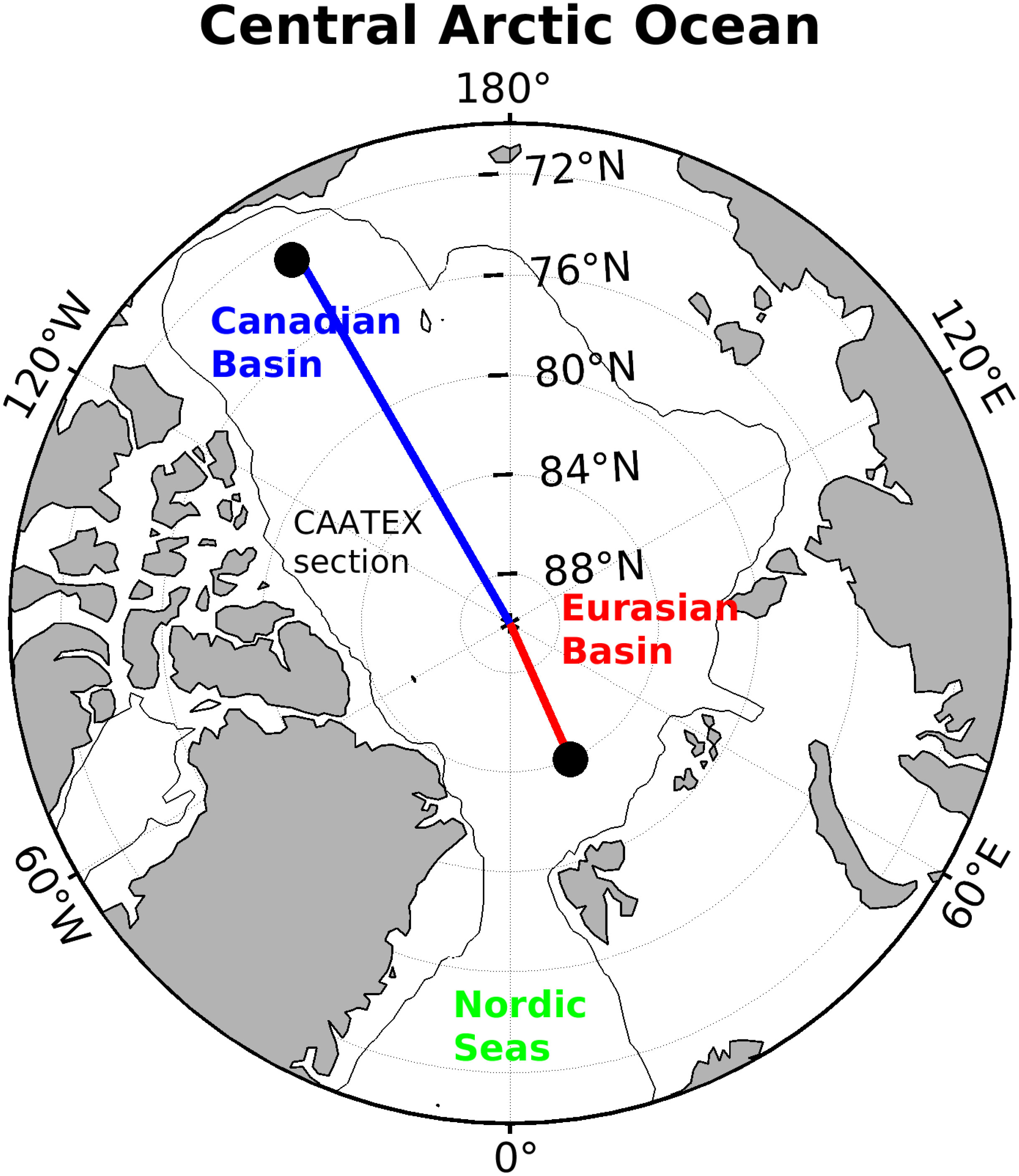
Figure 1 The focus for this study is the Central Arctic Ocean, which is here defined as the region embraced by the 500m isobath (grey thin curve) in the Arctic Ocean. The section across the Central Arctic Ocean is referred to as the CAATEX section in this study. The Eurasian (Canadian) part of the section is shown in red (blue).

A large amount of heat is transported from the Atlantic Ocean to the Arctic Ocean with the ocean currents, first across the Greenland-Scotland Ridge (about 285TW; long-term mean for 1900-2000 based on a sea ice-ocean model forced by a reanalysis atmosphere; Smedsrud et al., 2022), and then poleward though the Nordic Seas and the shallow Barents Sea (Figure 1). The ocean heat transport into the Arctic Ocean is pointed to as highly important in several recent studies using climate models; Pan et al. (2023) demonstrate that model spread in future projections is largely related to ocean heat transport via the Barents Sea, Madonna and Sandø (2022) describe large intermodel differences in the ocean heat transport which eventually propagate into the Arctic Ocean, and Docquier and Koenigk (2021) find that more realistic ocean heat transport towards the Arctic in climate models result in an earlier ice-free Arctic in September.

In this study, we focus on the upper Central Arctic Ocean, meaning ocean depth levels between 100-700m. The model spread is large in this layer compared to the rest of the water column (e.g. Khosravi et al., 2022), indicating challenges in modelling the water masses here. At these depths, typically the halocline, Atlantic Water and Pacific Water reside, where the halocline is locally formed in the Arctic in contrast to the advective Atlantic Water of subpolar origin (e.g. Rudels et al., 1999). The Atlantic Water is less influenced by the atmosphere and sea ice in the Arctic Ocean than the halocline and Polar Water. The halocline forms a boundary separating the fresh Polar Water on top and the saline Atlantic Water below, and thus, shows a sharp salinity gradient with depth. However, there are regional differences in the properties and distribution of these water masses. The Atlantic Water is warmer and sits higher in the water column in the Eurasian Basin than in the Canadian Basin (Figure 1), whereas the halocline is more pronounced in the Canadian Basin than in the Eurasian Basin (Timmermans and Marshall, 2020). In the Canadian Basin, a warming of the halocline is observed over the last three decades due to sea ice loss, which allows for more solar radiance to be absorbed (Timmermans et al., 2018). The Eurasian Basin is experiencing a warming in the core of the Atlantic Water (Polyakov et al., 2020), whereas an opposing trend is found in the Canadian Basin (e.g. Richards et al., 2022). Furthermore, over the last 40-50 years, the halocline has become fresher in the Canadian Basin, resulting in a stronger stratification. In contrast, in the Eurasian Basin, the stratification is weaker at halocline depths (with further references therein; Muilwijk et al., 2023).

Overall, the climate models project a warming in the Arctic Ocean at the end of this century, in particular for the Atlantic Water layer (Khosravi et al., 2022; Shu et al., 2022; Muilwijk et al., 2023). The future climate projections typically stretch to the year 2100 and several studies assess the changes in the long-term future (typically comparing the period 2081-2100 with the present era). However, with the rapid changes in the Arctic, it is also highly important to assess the Arctic Ocean in the near-term future (2021-2040) and the mid-term future (2041-2060), as defined in the IPCC Assessment Report (2021). Thus, in this study, we do not focus on the end of the century, but on the next three decades (2025-2055), encompassed in the near-to-mid term future. The manuscript is structured as follows: In Section 2, the material (CMIP6 models, ocean reanalysis, observations) and methods are introduced, in Section 3 we first evaluate the models and then we assess future changes in temperature and salinity for the upper Central Arctic Ocean. In Section 4, we discuss the results, and in Section 5, we conclude our study.

2 Materials and methods

In this study, we primarily analyze the annual mean temperature and salinity from the Central Arctic Ocean. Our data sources are CMIP6 ensemble members, ocean reanalysis, and hydrographic data from Arctic Ocean cruises along repeated lines. We evaluate the models over the period 1993-2010, and we assess simulated changes for the period 2025-2055.

2.1 CMIP6 model data

Data from the current generation of global climate model simulations are available through the most recent Coupled Model Intercomparison Project Phase 6 (CMIP6). The CMIP6 multi-model ensembles provide a range of different experiments where oceanographic variables are simulated for century long periods and provided as gridded data. For an efficient multi-model assessment on state-of-the-art climate models (CMIP6 models), model output data have been analyzed through the IS-ENES3 Analysis Platforms (https://is.enes.org/sdm-analysis-platforms-service/). In this way, heavy download of model output data is avoided, as model data can be directly accessed and analyzed on the IS-ENES3 Analysis Platforms. The model data that are included are described in Table 1 and include 13 different CMIP6 models: CAMS-CSM1-0 (Rong et al., 2019), CanESM5 (Swart et al., 2019), CESM2-WACCM (Danabasoglu et al., 2020), CIESM (Lin et al., 2020), CNRM-ESM2-1 (Séférian et al., 2019), EC-Earth3 (Döscher et al., 2022), GFDL-ESM4 (Dunne et al., 2020), INM-CM5-0 (Volodin and Gritsun, 2018), IPSLCM6A-LR (Lurton et al., 2020), MPI-ESM1-2-HR (Müller et al., 2018), MPI-ESM1-2-LR (Mauritsen et al., 2019), MRI-ESM2-0 (Yukimoto et al., 2019), and NorESM2-MM (Seland et al., 2020).

TABLE 1

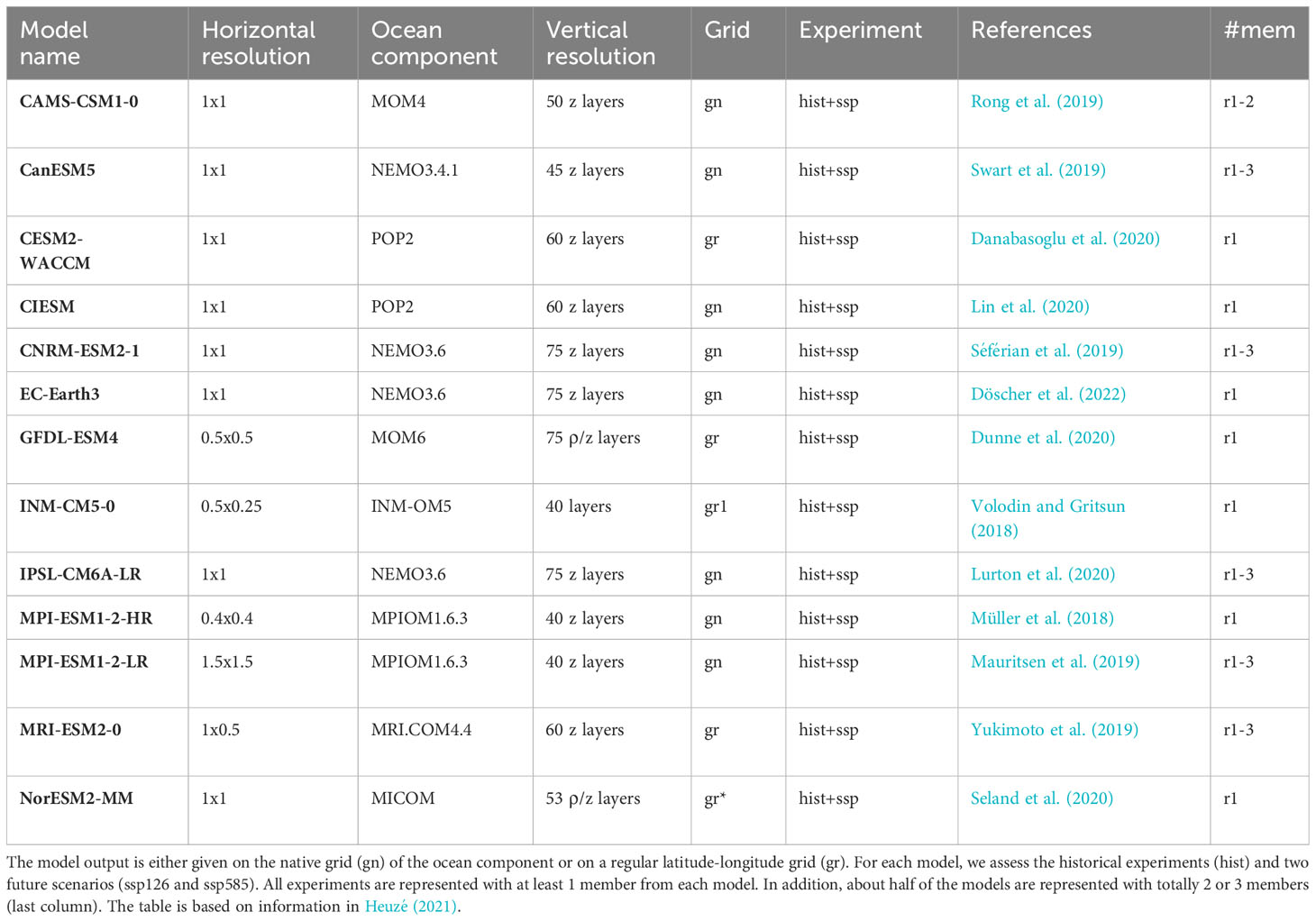
Table 1 Information about the CMIP6 models used in this study, including horizontal and vertical resolution of the ocean component.

We are using two different experiments from each of the CMIP6 model members: (1) historical experiment that covers the period 1850-2014 and (2) future scenarios (both ssp126 and ssp585) that cover the period 2015-2100 (O’Neill et al., 2016). The low end Shared Socioeconomic Pathways (ssp126) scenario has relatively weak global warming (0.5-1.5°C in the long-term; IPCC, 2021), which will lead to a CO2 level of 445ppm by 2100 (Meinshausen et al., 2020). The ssp126 experiment indicates an approximate radiative forcing of 2.6 W/m2 by 2100. The high end ssp585 experiment has strong global warming (2.4-4.8°C in the long-term; IPCC, 2021) and it is the only SSP scenario with emissions high enough to give a radiative forcing of 8.5 W/m2 by 2100. First, we evaluate the period 1993-2010 with ocean reanalysis data (described in the next subsection), and secondly, we assess the projected changes for the period 2025-2055. For the latter, we compare the two different scenarios, ssp126 and ssp585, to contrast a low global warming scenario with a more aggressive scenario.

As in two recent CMIP studies (Shu et al., 2019; Khosravi et al., 2022), our analysis is mainly focused on using the first member from each model experiment (in the CMIP6 archive this is referred to as the first realization; r1). The main reason for using one member from each model is that previous studies (e.g. Shu et al., 2022) have shown that the largest source of the model spread is model uncertainty and not internal variability (as expressed by the spread in members from one model). We have investigated the performance for additional members for some models, as described in the last column in Table 1 (using the second and third realization; r2 and r3). We find that performance of members from the same model is overall similar (not shown). The differences among the models are generally larger than the differences among the members. However, we note that the member spread for some models can be considerable. Similar results have been found in Zanowski et al. (2021), addressing the solid and liquid freshwater storage in the Arctic Ocean in CMIP6 models. In the rest of the manuscript, we apply the first member in all our analysis.

There are a number of recent studies that assess different aspects of CMIP6 models in the Arctic region, and we briefly list them in the following (the list is not exclusive). These studies focus on model biases related to Atlantic Water (Khosravi et al., 2022; Heuzé et al., 2023), model biases related to the deeper water masses (Heuzé et al., 2023), model spread in future projections of Atlantic Water warming (Khosravi et al., 2022; Muilwijk et al., 2023), model spread in future freshening of the halocline (Muilwijk et al., 2023), and in terms of future sea ice reduction (Notz and SIMIP Community, 2020; Årthun et al., 2021; Docquier and Koenigk, 2021). Furthermore, intermodel spread in poleward ocean heat transport has been assessed both in historical runs Madonna and Sandø (2022) and in future projections Pan et al. (2023). Regarding the latter, the study demonstrates that climate models with NEMO as the ocean model have in general a larger increase in ocean heattransport towards the Arctic than non-NEMO models. Interestingly, higher resolution versions of CMIP6 models during the historical period in general result in increased ocean heat transport compared to the coarser resolution version (Docquier et al., 2019).

2.2 The CAATEX section

Vertical sections across the Arctic Ocean have been used in several previous studies to assess the properties and distribution of different water masses (e.g. Ilıcak et al., 2016; Timmermans and Marshall, 2020; Heuzé et al., 2023). Indeed, there are regional differences, especially when comparing the Eurasian part of the section with the Canadian part of the section (Timmermans and Marshall, 2020, see their Figures 1 and 3). In our study, we also use a section cutting across the Eurasian Basin and the Canadian Basin (Figure 1). Here we call this the ‘CAATEX section’, as it has been defined in the US-Norwegian CAATEX project (Worcester et al., 2020). Our climate model study is part of this project. Observational (cruise) data is compared with ocean reanalysis data for the Eurasian part of the CAATEX section (red line; Figure 1). The cruise data applied in this study are described below (Section 2.4), and further information is given in a master thesis (Stallemo, 2022). Based on the CAATEX section, we vertically average temperature and salinity for five different depth layers (0-100m, 100-300m, 300-700m, 700-1500m, 1500-3000m). Our main focus is on the two uppermost layers, which we hereafter refer to as the Upper Layer (UL; 100-300m) and the Mid Layer (ML; 300-700m).

2.3 Model evaluation

In our CMIP6 model evaluation, we compare temperature and salinity averaged over the whole CAATEX section (for each depth layer) with ocean reanalysis data. In this way, we evaluate one single value (for each layer and variable) for each CMIP6 model. However, for a selection of the models, we display horizontal maps of temperature and salinity for both the Upper Layer and the Mid Layer. These maps show that there are indeed large regional differences in the models. We therefore introduce a new metric to evaluate the models; we compare their horizontal patterns of temperature and salinity with those from ocean reanalysis data. This method is described in detail in Section 2.6. Furthermore, we also complement our evaluation by temperature and salinity averaged over each basin. These values are obtained from previous CMIP6 studies (Khosravi et al., 2022; Heuzé et al., 2023), and are discussed for a selection of the models (details are given in Section 3.5).

2.4 Hydrography from ocean reanalysis data and cruise data in the Central Arctic Ocean

To evaluate the CMIP6 model data we use temperature and salinity from ocean reanalysis (ORA) data (Table 2). The ORA data are a multi-model mean (MMM) of 6 different reanalyses, providing monthly gridded data for the period 1993-2010. The ORA MMM is given on five different depth layers (same as described above), and we focus on the Central Arctic Ocean, i.e., where the water depth is exceeding 500m in the Arctic Ocean (Figure 1). This is the same region as studied in Uotila et al. (2019) (see their Figure 1A), which analyzed 10 different ocean reanalyses in the polar regions. The mask that is used to collect the data points where the depth is larger than 500m is shown in Figure 2. The data source used for the ocean depth is the 1 degree WOA13 bathymetry landsea-01.msk (https://www.nodc.noaa.gov/OC5/woa13/masks13.html). Note that the number of data points is reduced for the deeper layers (Figure 2). The ORA MMM and the individual ocean reanalyses are described in detail in Uotila et al. (2019) and a master thesis (Rautiainen, 2020). A main conclusion from the former study is that the ORA MMM compares well with observation-based climatology, as biases from individual ocean reanalyses are to significant extent cancelled out. In this study, we have therefore chosen to use the ORA MMM to evaluate CMIP6 models instead of using individual ocean reanalyses (the spread of the different ocean reanalyses provides good information on the observational uncertainty).

TABLE 2

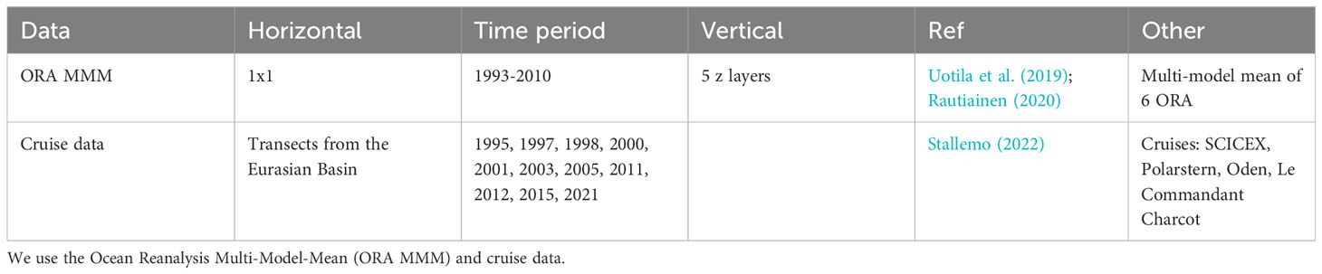
Table 2 Information about the ocean reanalysis and observational data used.

FIGURE 2

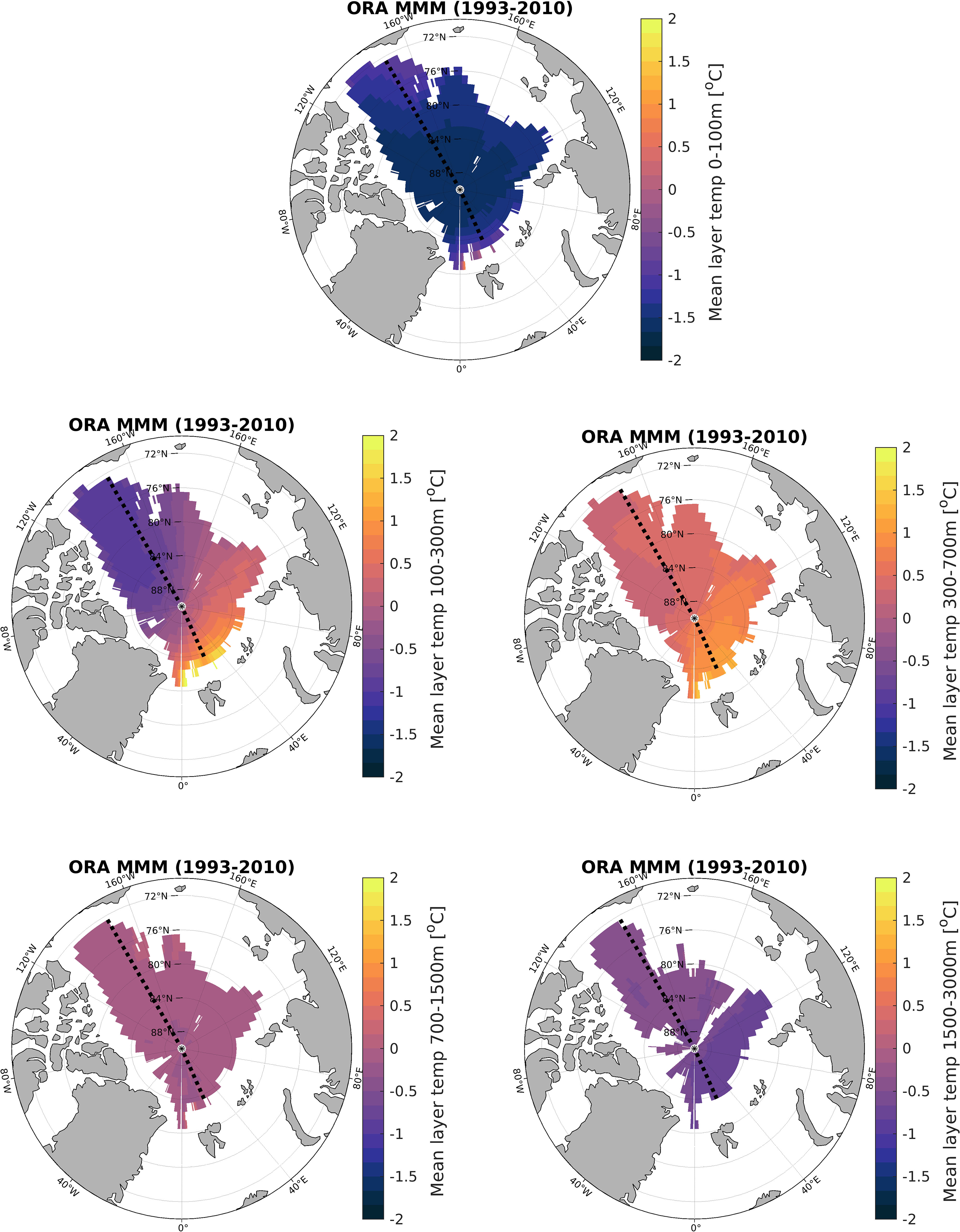
Figure 2 The ORA MMM is given on five different depth layers: 0-100m, 100-300m, 300-700m, 7001500m, 1500-3000m. The temperature in each layer is averaged over the time period 1993-2010. The maps also include the CAATEX section (black dashed line). The CMIP6 analysis will be carried out on these depths, with a particular focus on the Upper Layer (100-300m) and the Mid Layer (300-700m). ORA MMM is only shown for the Central Arctic Ocean (i.e., depths > 500m in the Arctic Ocean).

The ORA MMM product was compared with three observational hydrographic climatologies by (Uotila et al., 2019). Specifically, they used EN4.2.0.g10 (Good et al., 2013), World Ocean Atlas 2013 (WOA13; Locarnini et al., 2013; Zweng et al., 2013) and the Sumata Arctic hydrography (Sumata et al., 2018). Although the vertical resolution of the ORA MMM product is limited to five vertically integrated layers due to the ORA-IP protocol (Balmaseda et al., 2015), these ORA MMM layers rather realistically capture the main water masses and their features (see Figures 13 and 14 in Uotila et al., 2019). The most significant shortcoming is the too cold and fresh Atlantic Water layer in both Eurasian and Amerasian basins, attributed to weak Atlantic inflows into the Arctic Ocean. Importantly, the identified ORA MMM discrepancies are within the observational uncertainty, located for example between the Sumata and EN4 products, when comparing the vertically integrated layers.

To further support the use of the ORA MMM, we have compared the ORA MMM with hydrographic data from cruises in the Eurasian part of the CAATEX section (cruise data close to the section have been selected; Table 2). We find that the ORA MMM represents well the observed temperature of the Mid Layer (Figure 3A). The cruise data fall within the spread of the six different ocean reanalyses and close to the ORA MMM. In addition, we show that using two different definitions of Atlantic Water (T >0 or 300-700m) gives overall similar results (compare red and blue circles). Figure 3 also shows the temperature anomaly in the Eurasian part of the CAATEX section (B). The cruise data are mostly within the spread of the different ocean reanalyses and displays a weak positive trend over the period 1995-2021 (detrending the data gives a slightly lower temperature anomaly in year 2021). The ORA MMM also shows good results for salinity in the Mid Layer, and fairly good results for the Upper Layer (figures are provided in the Supplementary Figures). The spread of the different ocean reanalyses is larger for the Upper Layer than for the Mid Layer, but the cruise data still fall within the spread. In Section 3, we describe how the CMIP6 models compare to the ORA MMM.

FIGURE 3

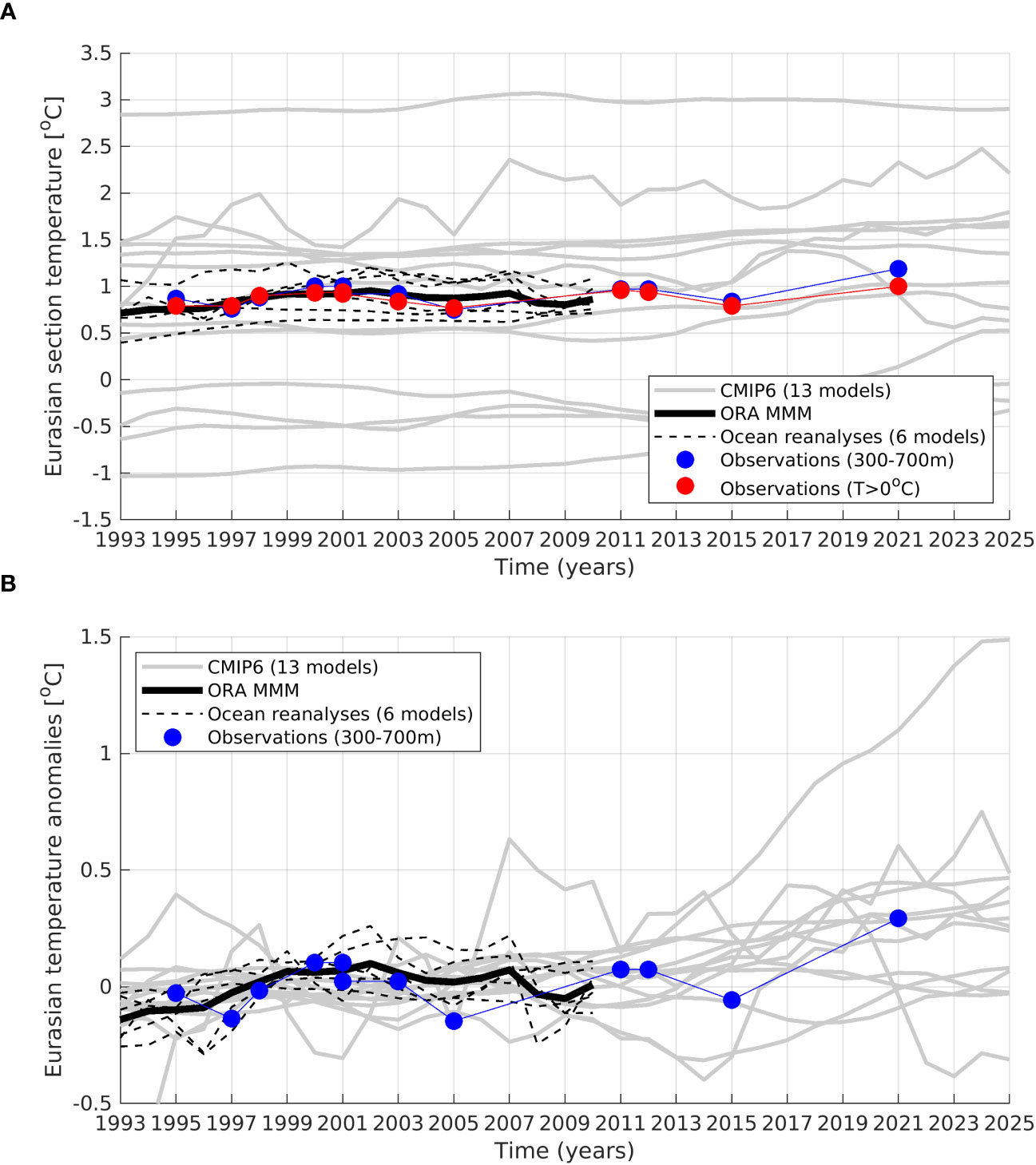
Figure 3 (A) The ORA MMM (black curve) is compared with cruise data (red and blue circles) in the Eurasian part of the CAATEX section. See Table 2 for information about the different data sets. All 13 CMIP6 models are included (grey curves). In this study, we use 300-700m to capture the Mid Layer, whereas T>0 is the typical definition for Atlantic Water in the Arctic Ocean. (B) Same as above, but for the anomalous temperature (the respective long-term mean for the period 1993-2010 has been removed for each data set, whereas the period 1995-2011 is used for the cruise data).

The monthly MMM includes these individual reanalyses: C-GLORS025v5 (Storto et al., 2016), MOVE-G2i (Toyoda et al., 2016), ORAP5 (Tietsche et al., 2017; Zuo et al., 2017), SODA3.3.1 (Carton and Giese, 2008), UR025.4 (Valdivieso et al., 2014) and ORAS5 (Zuo et al., 2019). These six reanalyses have been chosen as they provide data on monthly resolution. We chose to exclude one available reanalysis fitting the criteria due to unrealistic trends (Rautiainen, 2020). Five of the individual reanalyses has a horizontal resolution of 0.25°, whereas the sixth has a resolution of 1x0.3-0.5° (MOVE-G2i). All reanalyses are assimilating temperature and salinity from the observational-based data sets EN3v2a/EN4 or Word Ocean Database (WOD)/WOD13. The main data source for EN4 is WOD (Good et al., 2013). We find that several of the cruises that are listed in Table 2 are included in WOD. This means that the cruise data and the ORA MMM are not fully independent.

The main advantages of using the ORA MMM are that it performs well in the Arctic Ocean, and it has 3D temperature and salinity data providing a comprehensive coverage that can directly be compared with the CMIP6 model simulations. Statistical analysis, such as EN4, also provides 3D data fields (on 1x1° grid) and have been used in recent work for CMIP6 assessment in the Arctic Ocean (Shu et al., 2022). In this study, we use ORA MMM as this is a reanalysis product based on dynamical ocean models, and thus, the variables we use are dynamically consistent both in space and time in each of the individual ocean reanalyses. The ORA MMM is also based on models with a higher spatial resolution than EN4. More recent Arctic Ocean data, such as that from Ice Tethered Profilers (ITPs), are not included in EN4. The Arctic Ocean is a region with overall poor coverage of observations, and thus ocean reanalysis is a helpful tool in evaluating the performance of climate models.

2.5 ESMValTool

We use the Earth System Model Evaluation Tool (ESMValTool) to process output from the CMIP6 models described in Table 1. This tool eases the intercomparison of several CMIP6 models. We have used a recipe (https://docs.esmvaltool.org/en/latest/recipes/) to calculate the annual mean and to re-grid all model outputs to be comparable with the ORA MMM. This means that 3D ocean temperature and salinity from the CMIP6 models is interpolated to a 1x1^° horizontal grid for the following depths (in meter): 0, 20, 40, 60, 80, 100, 200, 300, 400, 500, 600, 700, 800, 900, 1000, 1100, 1200, 1300, 1400, 1500, 2000, 2500, 3000. Based on the re-gridded model data, we calculate the mean temperature and salinity for the five depth intervals provided by the ORA MMM: 0-100m, 100-300m, 300-700m, 700-1500m, 1500-3000m. The pattern correlation analysis (described below) is carried out on these depths.

2.6 Method of pattern correlation in the Central Arctic Ocean

In this study, we propose a new metric that considers the temporal evolution of the horizontal pattern of temperature (or salinity) of a specific layer (as shown in Figure 2). This horizontal pattern indicates the spread of water masses in the Central Arctic Ocean (e.g., such as Atlantic and Arctic water masses). In this case we are looking at the mean annual conditions and not the spread of anomalies with respect to a specific period.

To evaluate the performance of the models, we calculate the pattern correlation between the horizontal pattern from ORA MMM and from each of the 13 models. This metric is only applied for the Central Arctic Ocean and for each of the five depth intervals described above. The pattern correlation is calculated in the following way, including five steps: (1) For each time step (each year), apply the vertical mean for each of the five depth intervals as given in Section 2.5. (2) Select the area of the Central Arctic Ocean, by choosing the ocean grid cells where the ocean is deeper than 500m. (3) The selected 2D area is re-organized into a 1D-matrix (a vector). (4) The same procedure is applied for both ORA MMM and the CMIP6 models. (5) Finally, we correlate the two vectors, one from ORA MMM and one from the CMIP6 model. Note that the procedure above is repeated for each depth interval and for each time step. Performing the correlation for each time step, allows us to assess the time dependency of the pattern correlation. The results presented here are smoothed, i.e., the correlation is applied for a specific 5-year time window; running over the period 1993-2010. In the figures, we illustrate the median, minimum, and maximum correlation over time.

When extracting temperature and salinity from the Central Arctic Ocean (i.e., where the water depth is exceeding 500m), occasionally the models have NaN (Not a Number, i.e., a missing value) for some grid points in some layers. These NaNs have been replaced by using an average of neighbouring grid points before running the pattern correlation.

2.7 Water masses versus depth layers in climate models

As mentioned above, our main focus is on the two uppermost layers, the Upper Layer (UL; 100-300m) and the Mid Layer (ML; 300-700m). Although the halocline and Atlantic Water typically reside at these depths, we are not referring to these in our climate model study. Using a constant depth criteria for the definition of Atlantic Water and the halocline does not work for CMIP models in the Arctic. The reason is that these water masses are found at very different depths with large biases compared to observational based data (e.g. Ilıcak et al., 2016; Shu et al., 2019; Khosravi et al., 2022; Heuzé et al., 2023). Another approach, to circumvent this problem, is to use model dependent definitions. For instance, several studies use the maximum temperature in each vertical profile to capture the core of the Atlantic Water (e.g. Khosravi et al., 2022; Muilwijk et al., 2023). To capture the halocline is more challenging in climate models, but a recent study suggests a new metric by calculating potential energy available stored in stratification (Muilwijk et al., 2023). Using such model dependent definitions will help us to capture the correct water masses in each individual model. On the other hand, especially regarding Atlantic Water, it also means that we most likely compare water masses at very different depths when comparing the models. This could result in two models with Atlantic Water at different depths and at the same time showing a fairly realistic distribution of Atlantic Water in the Arctic Ocean. As a consequence, the models would achieve a high score with our metric (assessing horizontal patterns in the Central Arctic Ocean). The purpose with our metric is different: We want to give models a low score if one or two of the following conditions is the case: (1) simulated horizontal pattern not correct, (2) simulated depths of typical water masses are not correct. This means that our metric gives only a high score if both of the following is the case: the horizontal pattern needs to be realistic and typical water masses need to take place at realistic depths. Finally, we note that the results of our metric is dependent on the models’ horizontal pattern and vertical layering of water masses. Other metrics, might lead to a different ranking of the models. Thus, our selection of models that perform well might not work for all purposes. This is why we also compare our results with other metrics (Section 3.4) and compare our results with other CMIP6 studies (Section 3.5).

3 Results

In this section, we first assess the performance of the 13 models (Table 1) both in terms of their horizontal patterns and mean state, i.e., temperature and salinity averaged over the CAATEX section (3.1 and 3.2). Secondly, we quantify the model spread in temperature and salinity anomalies over the period 2025-2055 (3.3). We then compare climate sensitivity of the models together with a few other key criteria in the Arctic (sea ice sensitivity, ocean heat transport, halocline, and deeper water masses) based on results from the literature (3.4 and 3.5). Finally, based on our model evaluation and the climate sensitivity, we sub-select models to assess projected changes for the period 2025-2055 (3.6). As described in Section 2, our focus is on the Upper Layer (100-300m) and the Mid Layer (300-700m). These two layers show the largest gradients in the Central Arctic Ocean, whereas the other three layers show more homogenous patterns (Figure 2). Thus, the model evaluation for the Polar Layer (0-100m), the Deep Layer (700-1500m), and Bottom Layer (1500-3000m) are not discussed (figures are provided in the Supplementary Figures).

3.1 Performance of CMIP6 models in simulating temperature in Upper and Mid layers

We find that there is a large spread both in the pattern correlations and the mean temperature (illustrated by the horizontal spread of the coloured circles; Figure 4). For instance, the ORA MMM has a mean value of about 0.5°C for the Mid Layer for the period 1993-2010, whereas the coldest model has a mean value of less than -1^°C and the warmest model a value of almost 2.5°C. The pattern correlations range from 0.2 to above 0.9 for the Upper Layer (colored lines; Figure 4). Similar values are found for the Mid Layer, except two models that have negative correlations (not shown). Some of the models show relatively large temporal variability in the pattern correlation (e.g., INM-CM5-0 and CNRM-ESM2-1; compare extent of vertical lines). There is little time dependency of the temperature patterns of the ORA MMM (black vertical line). To show this, ORA MMM is correlated with itself by keeping one pattern fixed (an average over the first 5 years) and the other pattern varies with time, as described in Subsection 2.6. Note that the interannual variability in the ORA MMM is likely smoothed, because of the averaging over six different ocean reanalyses (e.g., see Figure 3B).

FIGURE 4

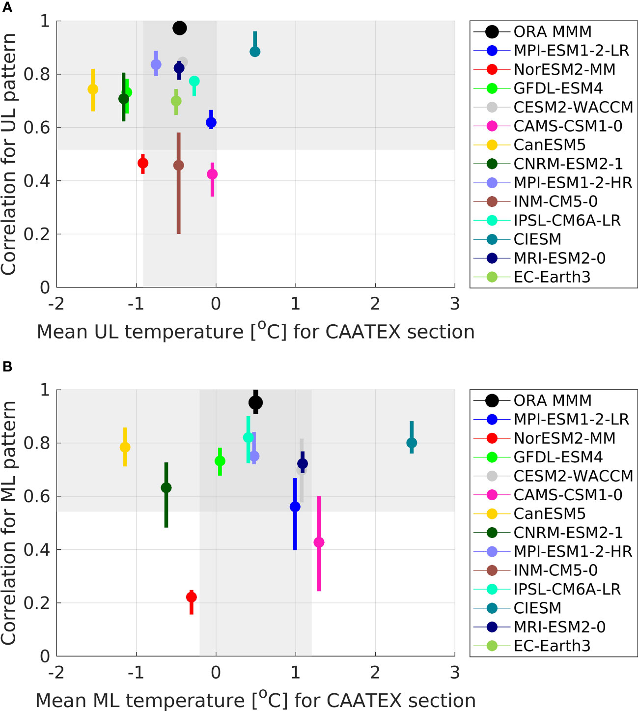
Figure 4 Correlation of temperature patterns from the CMIP6 models and that from the ORA MMM for the time period 1993-2010 (coloured circles and lines) in two different layers: (A) the Upper Layer (UL; 100-300m) and (B) the Mid Layer (ML; 300-700m). The correlation is performed for different time slices, where the variation in the correlations is seen by the vertical lines (showing the minimum and maximum correlation). The position of the circle gives the median correlation. The circle shows also the mean temperature for the CAATEX section. The grey bands show significant correlations at 95% level and mean values within 10*STD of ORA MMM (temporal STD of ORA MMM for 1993-2010). Note that two models are not shown for the Mid Layer, as they have negative pattern correlations.

The models that perform the best in one specific layer are not necessarily the same models that perform the best in another layer. For instance, CESM2-WACCM and MPI-ESM1-2-HR perform well in terms of temperature in the Upper Layer (correlations of 0.85 and 0.84, respectively), whereas MPI-ESM1-2-HR and IPSL-CM6A-LR are showing better results for temperature in the Mid Layer (Figure 4; correlations of 0.75 and 0.82, respectively; CESM2-WACCM and MRI-ESM2-0 with correlations 0.70 and 0.72, respectively). However, we find that IPSL-CM6A-LR and MRI-ESM2-0 are also showing good results in the Upper Layer (0.77 and 0.82, respectively). We further analyze these four models, by comparing their spatial distribution of temperature in the Upper and Mid layers (Figure 5). Note that temperature is shown for all grid points, i.e., the mask shown in Figure 2 has not been applied. Among the models, MPI-ESM1-2-HR has the strongest temperature gradient when crossing the Arctic Ocean from the Eurasian Basin to the Canadian Basin (also stronger than that shown by ORA MMM). Warm water from the south also seems to extend further into the Eurasian Basin in this model. The gradient in IPSL-CM6A-LR is weaker than that shown by ORA MMM.

FIGURE 5

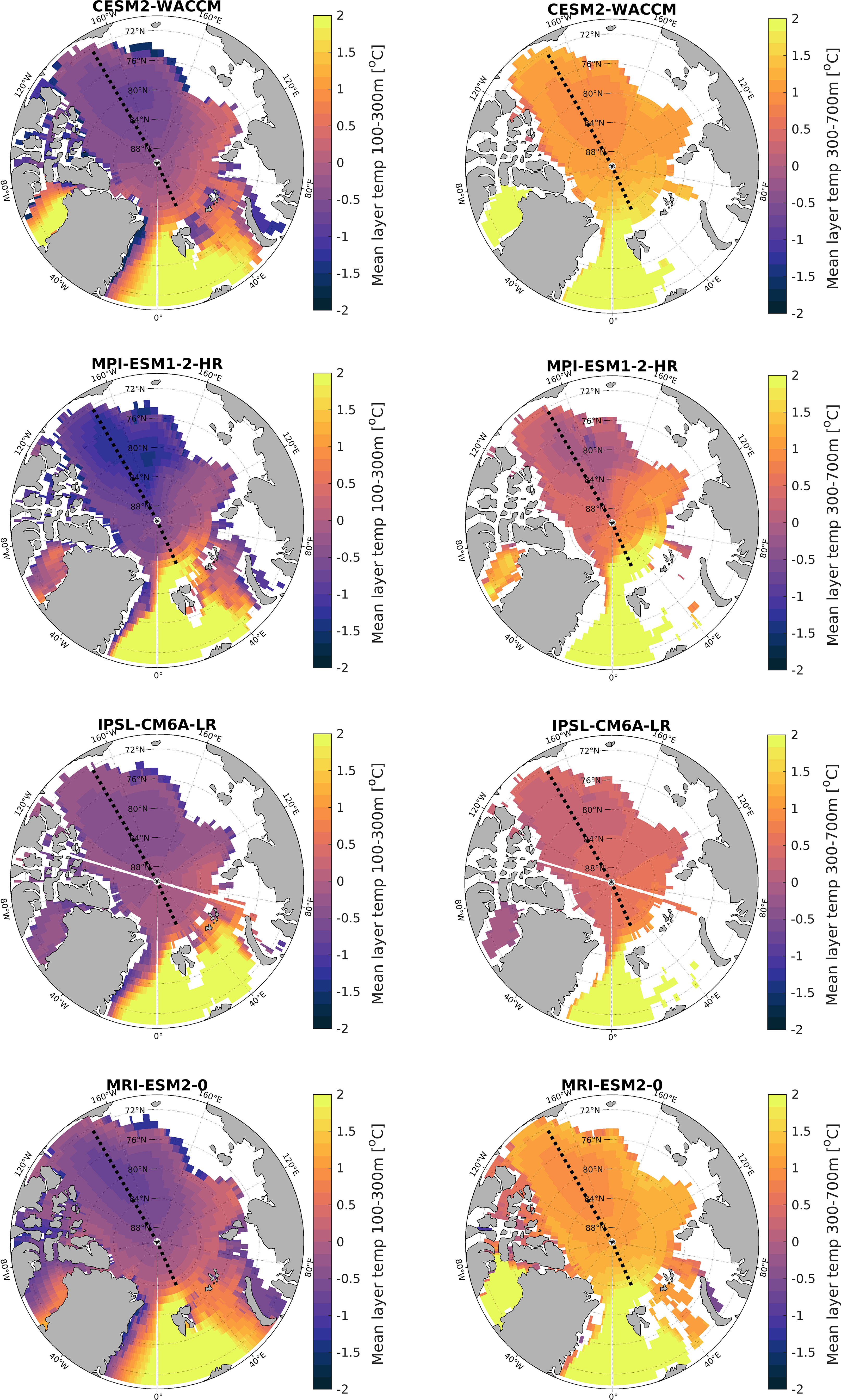
Figure 5 Average temperature from four CMIP6 models over the time period 1993-2010 in the Upper Layer (UL; left panel) and the Mid Layer (ML; right panel).

3.2 Performance of CMIP6 models in simulating salinity in Upper and Mid layers

Considering salinity in the same way as temperature, we find again a large spread in the pattern correlations but with a somewhat reduced range (correlations mainly between 0.4 and 0.9; Figure 6). In general, the time dependency of the pattern correlation seems to be smaller for salinity than for temperature, especially for the Mid Layer. This difference in the pattern correlation for salinity and temperature might be related to the fact that salinity is in general more conservative than temperature. In this way, the salinity pattern in the climate models, assumed to be mainly caused by ocean circulation (especially in the Mid Layer), is to a less extent modified by mixing among different water masses.

FIGURE 6

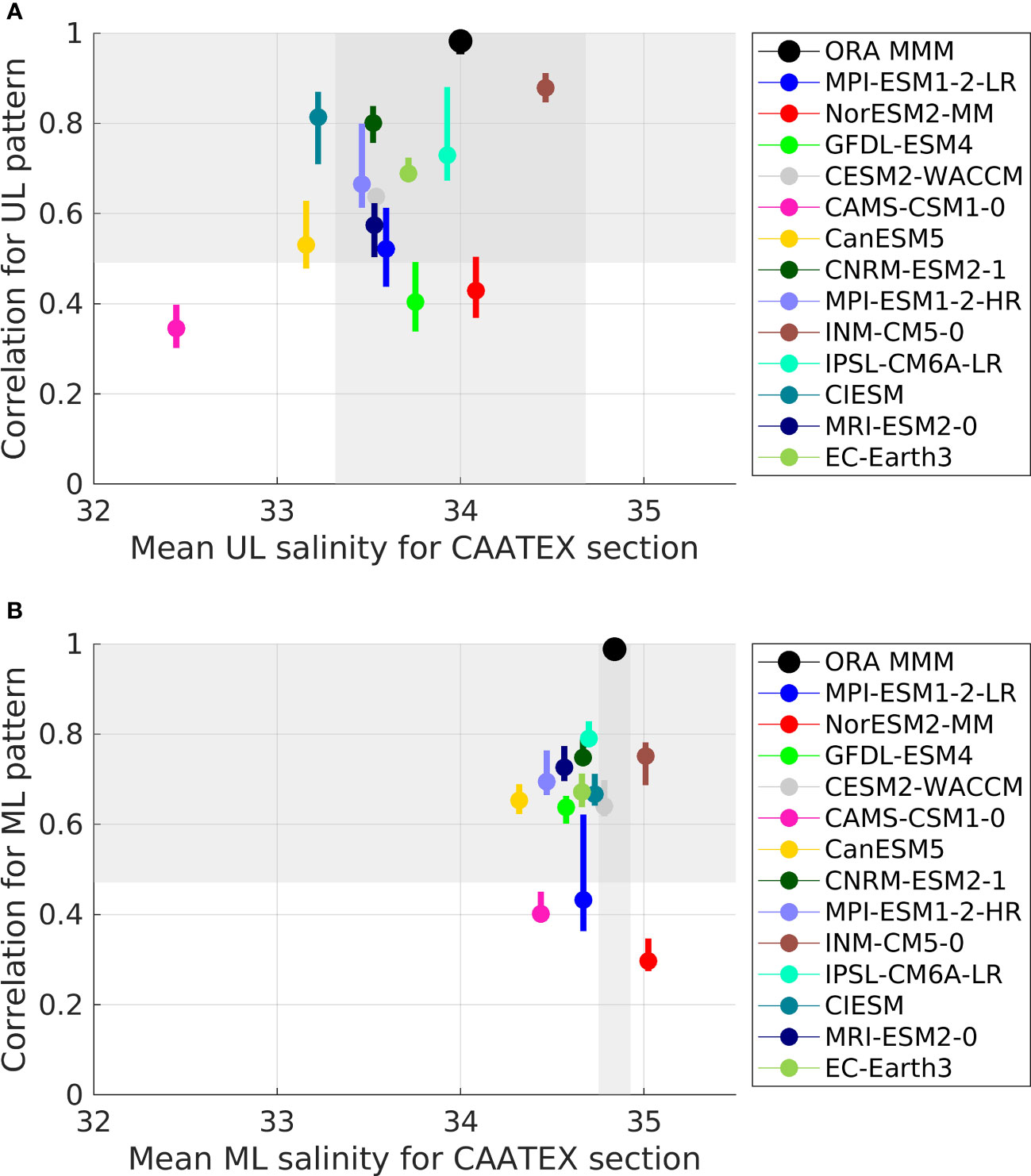
Figure 6 Correlation of salinity patterns from the CMIP6 models and that from the ORA MMM for the time period 1993-2010 (coloured circles and lines) in two different layers: (A) the Upper Layer (UL; 100-300m) and (B) the Mid Layer (ML; 300-700m). The correlation is performed for different time slices, where the variation in the correlations is seen by the vertical lines (showing the minimum and maximum correlation). The position of the circle gives the median correlation. The circle shows also the mean salinity for the CAATEX section. The grey bands show significant correlations at 95% level and mean values within 10*STD of ORA MMM (temporal STD of ORA MMM for 1993-2010).

We find that IPSL-CM6A-LR is showing the best results regarding salinity in the two layers (Figure 6; correlations above 0.75). However, there are also five other models that show overall good results for salinity (CESM2-WACCM, MPI-ESM1-2-HR, MRI-ESM2-0, CNRM-ESM2-1, and EC-Earth3). INMCM5-0 is not included because of its overall low pattern correlation for temperature (Figure 4). We further analyze the six models, by comparing their spatial distribution of salinity in the Upper and Mid layers (Figure 7; CNRM-ESM2-1, and EC-Earth3 are shown in the Supplementary Files). We find that the fresh Upper Layer in the Canadian Basin expands into the Eurasian Basin to a large degree in three of the models (CESM2-WACCM, MPI-ESM1-2-HR, and MRI-ESM2-0), both compared to the other models and compared to ORA MMM. In CNRM-ESM2-1 and EC-Earth3, the Upper Layer is very fresh in the Canadian Basin compared to the other models and ORA MMM.

FIGURE 7

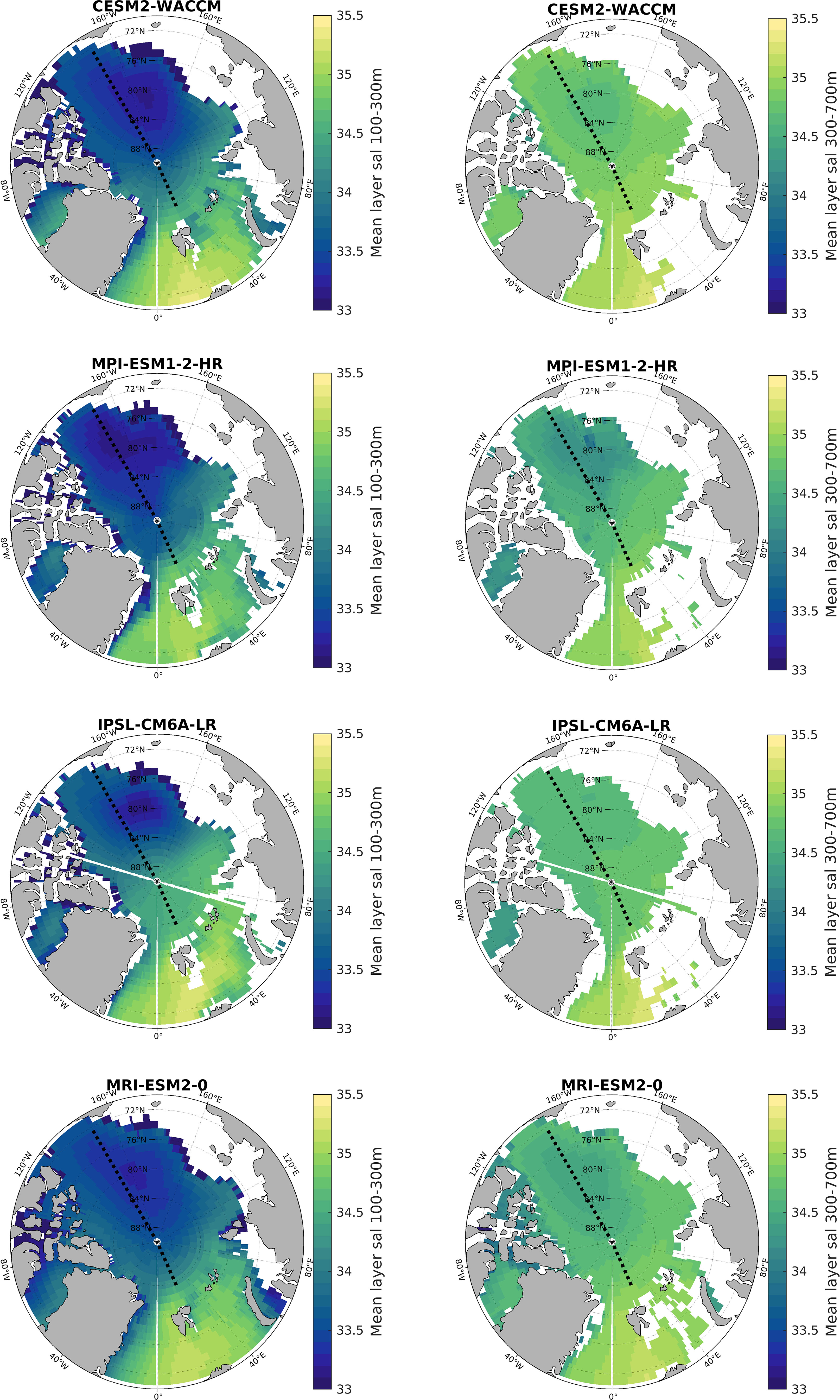
Figure 7 Average salinity from four CMIP6 models over the time period 1993-2010 in the Upper Layer (UL; left panel) and the Mid Layer (ML; right panel).

Analyzing salinity in the Mid Layer in the same six models (Figure 7 and Supplementary Files), we find it more challenging to identify which models are performing best. The gradient across the Arctic Ocean is weak in the ORA MMM (compared to the gradient in the Upper Layer). The six models show various gradients, some weaker and some stronger than the ORA MMM. Most models also show a minimum salinity in the central Canadian Basin, which is not found in ORA MMM. Some models show this feature clearly (e.g., CESM2-WACCM, MRI-ESM2-0, CNRM-ESM2-1), whereas it is not as distinct for IPSLCM6A-LR. The ORA MMM pattern might be smoothed by averaging across six different ocean reanalyses. However, the salinity minimum displayed by the models is not clearly seen in the salinity maps using data from the Atlantic Water core (Richards et al., 2022), which typically sits in the depth range of the Mid Layer (300-700m).

In summary, assessing the performance in the Central Arctic Ocean of the CMIP6 model simulations used in this study, we find four models with fairly good results (CESM2-WACCM, MPI-ESM1-2-HR, IPSLCM6A-LR, MRI-ESM2-0) compared to the other models. Overall, MPI-ESM1-2-HR, IPSL-CM6A-LR shows slightly better results than CESM2-WACCM, MRI-ESM2-0.

3.3 Large model spread in CMIP6 projections for the Central Arctic Ocean (2025-2055)

The 13 CMIP6 models show a large spread in the temperature anomalies projected for the period 20252055 in the CAATEX section (grey curves, Figure 8). Considering the CMIP6 MMM (dashed curves; Figure 8), we find a warming of 0.6^°C and 0.7°C in 2045-2055 (compared to 1993-2010) in the Upper and Mid layers, respectively, for the low end (ssp126) scenario. This increases to 0.8°C and 0.9°C, respectively, in the high end (ssp585) scenario. In previous subsections (3.1 and 3.2), we have also seen that there is a considerable spread in the mean state of the CMIP6 models (illustrated by the horizontal spread of the coloured circles; Figures 4, 6).

FIGURE 8

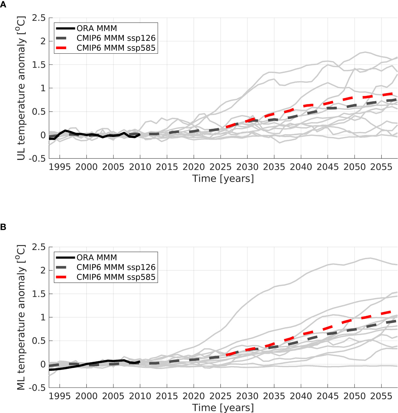
Figure 8 (A) Temperature anomalies of the Upper Layer (UL) for the CAATEX section. All 13 CMIP6 models are included (ssp126; grey curves), and CMIP6 MMM ssp126/ssp585 (grey/red dashed curve) is compared with the ORA MMM (black curve). Anomalous temperature is calculated by removing the respective long-term mean for the period 1993-2010 for each data set. (B) Same as above, but for the Mid Layer (ML).

We have quantified the model spread for both the mean state and the anomaly temperature and salinity (Figure 9). In the reference period (1993-2010; ORA MMM is shown as horizontal lines), we find that the CMIP6 spread for the mean state is much larger than that for the anomalies (compare solid and dashed curves, respectively). This is seen for temperature and salinity in both layers. The largest CMIP6 spread is found in the mean temperature (salinity) in the Mid (Upper) Layer. Most interestingly, the CMIP6 spread for the temperature and salinity anomalies ramp up during the next two decades (2025-2045). The maximum model spread is reached in the following decade (2045-2055) with a standard deviation at least 10 times higher than in 1993-2010. At this stage, the CMIP6 spread for temperature and salinity anomalies is almost reaching that of the mean state (compare dashed and solid curves, respectively, in 2045-2055). Similar results are found for the temperature and salinity anomalies in the ssp585 scenario (red and magenta curves; Figure 9), but with slightly larger (smaller) standard deviation for temperature (salinity). The smaller standard deviation is only found in the Upper Layer.

FIGURE 9

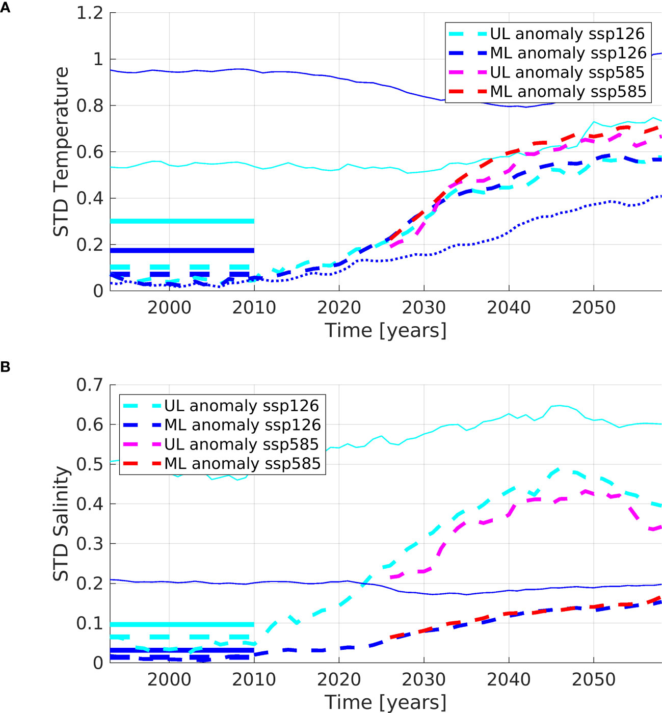
Figure 9 (A) Standard deviation (STD) of Upper Layer (UL; light blue) and Mid Layer (ML; blue) temperature in the CAATEX section. The STD is shown for each year based on 13 CMIP6 models (thin solid lines). The STD is also shown for anomalous temperature (dashed lines), which are calculated by removing the respective climatology for the time period 1993-2010. The time-average STD based on 6 ORA are shown as horizontal lines. The STD is clearly reduced for ML temperature anomaly (ssp126; blue dotted line) when applying 9 sub-selected CMIP6 models (see description in 3.6). (B) Same as above, but for salinity instead.

Now that we have seen the large CMIP6 spread for the anomalies in the future projections, we aim in the following subsections to reduce this spread considering the performance of the models in the Arctic Ocean and their climate sensitivity.

3.4 Assessing CMIP6 performance and climate sensitivity to sub-select models

In 3.1 and 3.2, we found four models that show better results in the Central Arctic Ocean than the other models. However, we acknowledge that the performance of the CMIP6 models depends on the region, variable, and period under consideration. Thus, to provide a more robust evaluation of the models, we here describe the performance of the CMIP6 models with respect to other key metrics, such as Arctic sea ice sensitivity, and northward ocean heat transport across the Greenland-Scotland Ridge (Figure 10). A similar approach was done in Docquier and Koenigk (2021), where a range of criteria were assessed in CMIP6 models before sub-selecting models to assess future projections of Arctic sea ice. They found that the sub-selected models reached a summer ice-free Arctic faster than the multi-model mean (MMM).

FIGURE 10

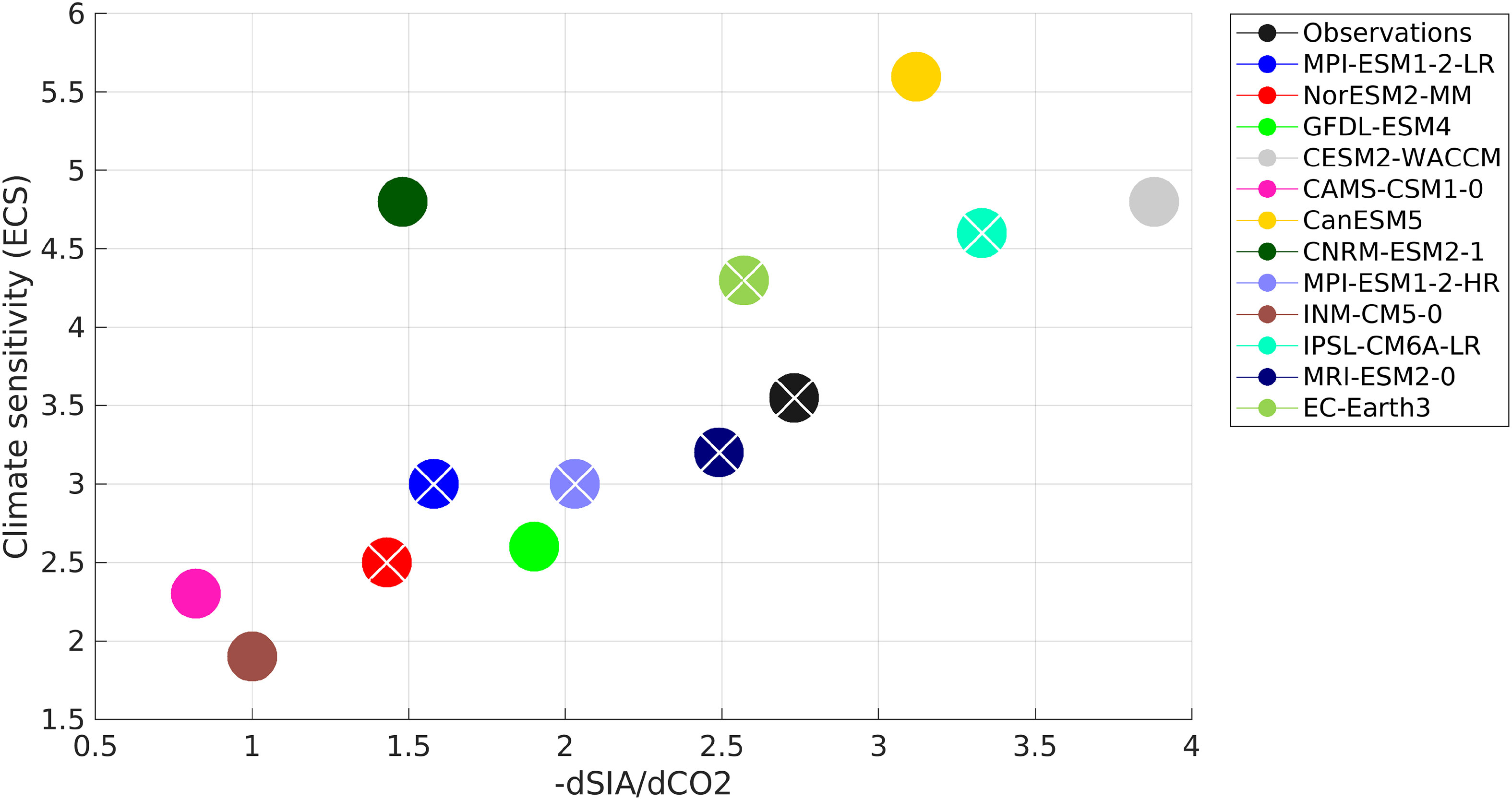
Figure 10 Relationship between the sensitivity of September Arctic sea ice to CO2 emissions (dSIA/dCO2) and Equilibrium Climate Sensitivity (ECS). The different models are indicated by different colours. The amount of ocean heat transport across the Iceland-Scotland Ridge is discussed in the text for some of the CMIP6 models (only provided for those models marked with a white cross). The observed value of dSIA/dCO2 is illustrated by the black circle (the ECS is set to the mean of the 13 models). Simulated and observed values are based on the literature (sea ice sensitivity; Notz and SIMIP Community, 2020, climate sensitivity; Meehl et al., 2020, ocean heat transport; Madonna and Sandø, 2022). CIESM is not included, as numbers were not provided for this model in the references given here.

In Figure 10 we have included the Equilibrium Climate Sensitivity (ECS) of the CMIP6 models and their sensitivity of September Arctic sea ice area to CO2 emissions. All numbers in Figure 10 are based on the recent literature, focusing on either Arctic sea ice area (Notz and SIMIP Community, 2020) or ECS (Meehl et al., 2020). ECS means how many degrees the global surface air temperature will increase after a doubling of CO2 (after the system is in balance). There seems to be a positive relationship between ECS and dSIA/dCO2. This suggest that the ESC, although a global metric, matter for the Arctic.

Ocean heat transport towards the Arctic is also an important metric in the assessment and intercomparison of CMIP6 models (Madonna and Sandø, 2022). For instance, the ocean heat transport through the Barents Sea Opening has a strong influence on the March sea ice area, whereas the sea ice area in September is more related to bottom melting of sea ice within the Central Arctic Ocean (Sandø et al., 2014). An assessment for the ocean heat transport across the Iceland-Scotland Ridge has been provided for about half of the models included in this study (Madonna and Sandø, 2022, models marked with a white cross in Figure 10). We discuss below the ocean heat transport values together with the sensitivities for only four models.

We take a closer look at the four models with relatively good performance in the Upper and Mid Layers (MPI-ESM1-2-HR, IPSL-CM6A-LR, CESM2-WACCM, MRI-ESM2-0). We find that both IPSL-CM6A-LR and CESM2-WACCM have a relatively high climate sensitivity (above 4.5; Figure 10), whereas MPI-ESM1-2-HR and MRI-ESM2-0 have a more moderate climate sensitivity (around 3). IPSL-CM6A-LR and CESM2-WACCM have also too high sea ice sensitivity compared to observations, whereas the sea ice sensitivity in MPI-ESM1-2-HR is too low. MRI-ESM2-0 compares well with the observed sea ice sensitivity. The ocean heat transport across the Iceland-Scotland Ridge in MPI-ESM1-2-HR (239.7 TW) compares well with observations (231 TW), whereas the heat transport is too large in IPSL-CM6A-LR and MRI-ESM2-0 (326.6 TW and 303.7 TW, respectively).

3.5 Mean state conditions in the Arctic Ocean for sub-selected models

The previous section dealt with somewhat “external” factors to the Upper and Mid layers (such as sea ice, climate sensitivity, and ocean heat transport measured outside the Arctic Ocean), we now zoom again in on the mean state in the Arctic Ocean. We compare our results with those recently reported by several other CMIP6 studies (e.g. Heuzé et al., 2023; Muilwijk et al., 2023). Muilwijk et al. (2023) evaluated the halocline in detail in a suite of CMIP6 models, whereas Heuzé et al. (2023), in the same suit of CMIP6 models, evaluated the water masses from the Atlantic Water and down to the bottom waters. These studies did not point to specific models performing better than others in the Arctic Ocean. We therefore continue to use our four sub-selected models (MPI-ESM1-2-HR, IPSL-CM6A-LR, CESM2-WACCM, MRI-ESM2-0) and further discuss their performance in the Arctic Ocean based on these studies.

Interestingly, IPSL-CM6A-LR is the only model that has a fairly realistic difference in the mean stratification between the Canadian Basin and Eurasian Basin (Muilwijk et al., 2023, their Figure 3). On the other hand, CESM2 (as CESM2-WACCM is not included in their study) shows too weak stratification in the Canadian Basin compared to observations, and too strong stratification in the Eurasian Basin. Similarly, MPI-ESM1-2-HR and MRI-ESM2-0 have also too weak stratification in the Canadian Basin, but their mean stratification is more realistic in the Eurasian Basin. These results regarding the halocline appears to be consistent with our results; IPSL-CM6A-LR is showing the best results, both regarding the salinity pattern and the mean salinity, in both the Upper and Mid layers (Figure 6).

Khosravi et al. (2022) have evaluated the core temperature and depth of Atlantic Water in both the Canadian Basin and Eurasian Basin (their Figure 2). IPSL-CM6A-LR has a realistic Atlantic Water temperature in the Canadian Basin, but too low temperature in the Eurasian Basin. Similarly, MPIESM1-2-HR has a realistic temperature in the Canadian Basin, but slightly too high in the Eurasian Basin. On the other hand, both MRI-ESM2-0 and CESM2-WACCM have way too high temperatures in both basins and the depth of the core is overly deep. IPSL-CM6A-LR also has a too deep core, and also MPI-ESM1-2-HR, but to a less degree. These results are overall consistent with those in Heuzé et al. (2023), assessing the Atlantic Water in all of the four basins separately (Nansen, Amundsen, Makarov, Canada). Only difference is that MPI-ESM1-2-HR is slightly too cold in the two Eurasian basins, instead of slightly too warm, as described above. Indeed the above findings are in line with our results for the temperature in the Mid Layer, with CESM2-WACCM and MRI-ESM2-0 being warmer than MPI-ESM1-2-HR and IPSL-CM6A-LR (Figure 4B).

The above results for the Atlantic Water links well with the CMIP6 conditions in the Fram Strait. Both MRI-ESM2-0 and CESM2 overestimates to a large degree the temperature below approximately 500m (Heuzé et al., 2023). The temperature at these depths is also too high in MPI-ESM1-2-HR and IPSLCM6A-LR compared to observations, but to a less degree. Additionally, the depth of the core in the latter two models appears to sit higher in the water column than in the other two models (Heuzé et al., 2023). However, all studied models in (Heuzé et al., 2023) have problems in accurately representing inflows and outflows in the Fram Strait, resulting in biases in the ocean heat transports into the Arctic Ocean. Assessing the ocean heat transport a bit further south, Docquier and Koenigk (2021) find that MPI-ESM1-2-HR, IPSL-CM6A-LR, MRI-ESM2-0 are part of the 8 models (out of 16 models) that are closest to the observed ocean heat transports across both 70°N in the Atlantic and 60°N in the Pacific.

In general, MPI-ESM1-2-HR and IPSL-CM6A-LR seem to perform better than MRI-ESM2-0 and CESM2-WACCM, according to the metrics presented above. However, all of the fours models appears to do fairly well in the Arctic Ocean compared to other CMIP6 models. For instance, Khosravi et al. (2022) show that several models have far too low temperature of the Atlantic Water core. Interestingly, Heuzé et al. (2023) find that only six models are likely to have polynyas in the Kara Sea, a process important for dense water formation, where four of these are our sub-selected models. In the next subsection, we examine future estimates of temperature and salinity for all four models, but with more emphasis on the two first models.

3.6 An attempt to constrain CMIP6 future projections for the Central Arctic Ocean

We assess the projected temperature and salinity in the sub-selected models (MPI-ESM1-2-HR, IPSL-CM6A-LR, CESM2-WACCM, MRI-ESM2-0) for the period 2025-2055 averaged over the CAATEX section (Figure 11). We clearly see that IPSL-CM6A-LR has a larger warming than the other three models, in both the Upper and Mid Layer. This may be a result of their different climate sensitivity (Figure 10). However, both IPSL-CM6A-LR and CESM2-WACCM have relatively high climate sensitivity, and CESM2-WACCM shows changes more comparable to the two other models with a more reasonable climate sensitivity. In addition, IPSL-CM6A-LR has a large increase in the salinity in the Upper Layer, whereas the other three models show a freshening. In the Mid Layer, the salinity changes are small compared to those in the Upper Layer. MPI-ESM1-2-HR shows a weak salinification, and the rest of the models show a weak freshening.

FIGURE 11

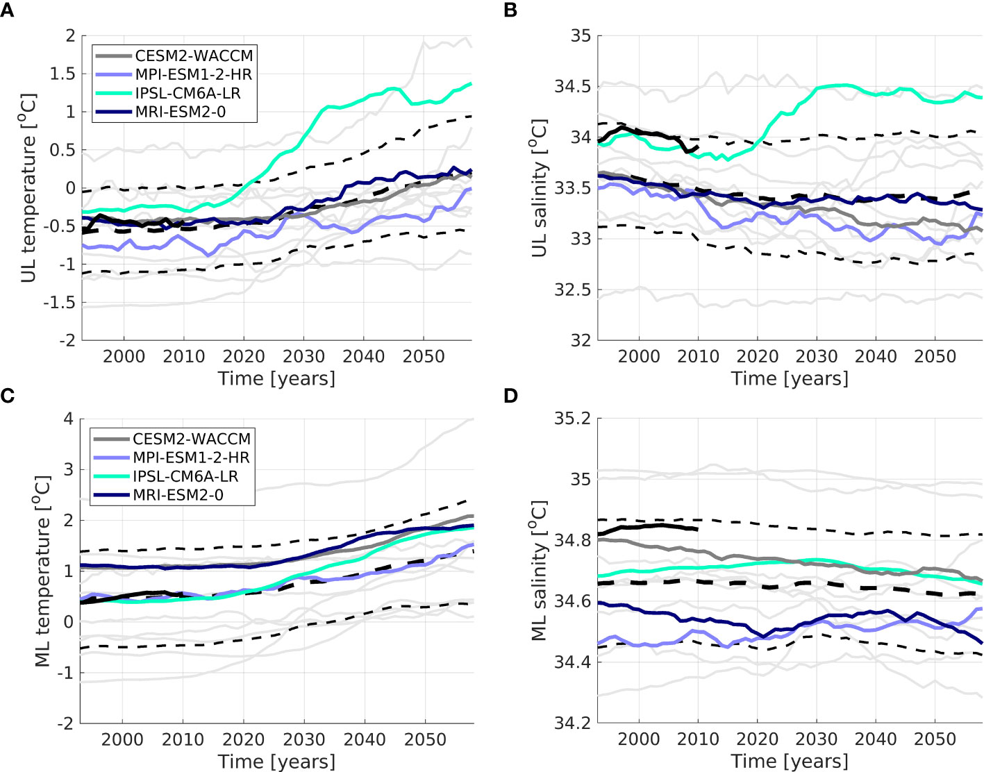
Figure 11 (A) Temperature and (B) salinity of the Upper Layer (UL) for the CAATEX section. All 13 CMIP6 models are included (ssp126; grey curves). Some of the models are highlighted with colours. The CMIP6 MMM and STD are also included (dashed black curves), together with the ORA MMM (solid black curve). (C, D) Same as above, but for the Mid Layer (ML). Note that the scale of the y-axis varies.

We also test another approach to reduce the model spread in the future projections. We have selected those models with relatively high horizontal or vertical resolution (i.e., we remove the models with less than 54 vertical layers and horizontal resolution 1x1° or lower). Based on this approach we reduce from 13 to 9 CMIP6 models. The STD is clearly reduced for Mid Layer temperature anomaly when applying these 9 CMIP6 models compared to applying all models (Figure 9; blue dotted line in upper panel). Although the STD is expected to decrease with a smaller sample of models, we also find a substantial reduction in the difference between the models with maximum and minimum values (13 models has a mean difference of 2.2°C for the period 2045-2055, whereas 9 models has a mean difference of 1.1°C for the same period).

To assess the results based on our different sub-selections, we compare the projected temperature and salinity changes for the period 2045-2055 across the four models and the multi-model mean based on 13 (MMM13) or 9 (MMM9) models (Figure 12; black bars). We find that the MMM does not change much when changing the number of models, showing a warming of 0.63°C (0.67°C) in the Upper Layer for ssp126 using MMM13 (MMM9). Similarly, the Mid Layer for ssp126 shows a warming of 0.75°C (0.72°C) using MMM13 (MMM9). Now, considering the four models, we find that CESM2-WACCM and MPI-ESM1-2-HR show similar results for the ssp126 scenario with less warming and larger freshening in the Upper Layer compared to the MMM. MRI-ESM2-0 shows similar results as the MMM, whereas IPSLCM6A-LR shows a large warming and a salinification in the Upper Layer. In the Mid Layer, three of the models are like the warming in the MMM, whereas the salinity changes are overall small. IPSL-CM6A-LR shows again a large warming.

FIGURE 12

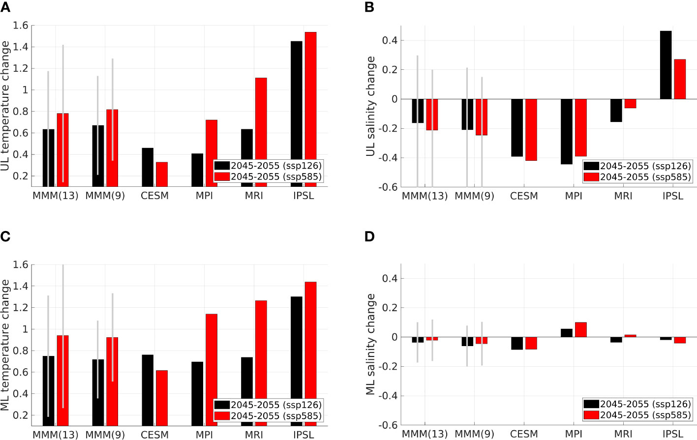
Figure 12 Projected (A) temperature and (B) salinity changes in the Upper Layer (UL) during the period 2045-2055 for the CAATEX section. Changes are shown for the CMIP6 MMM based on 13 and 9 models (1STD is shown as grey vertical lines), and for four different models (CESM2-WACCM, MPI-ESM1-2-HR, MRI-ESM2-0, IPSL-CM6A-LR). Changes are compared to the reference period 1993-2010 and are shown for two scenarios: ssp126 (black bars) and ssp585 (red bars). (C, D) Same as above, but for the Mid Layer (ML).

In the ssp585 scenario, the MMM13 and MMM9 are still similar, but there are overall larger differences among the four models for temperature (Figure 12; red bars). We find increased warming in the following order (values are here only given for the Upper Layer): CESM2-WACCM (0.33°C), MPI-ESM1-2-HR (0.72°C), MRI-ESM2-0 (1.11°C), c (1.54°C).

As described above, MPI-ESM1-2-HR and IPSL-CM6A-LR show overall better performance than the two other models, and we therefore describe these models in some more detail. In addition, IPSL-CM6A-LR appears to better represent salinity in both the Upper and Mid layers than MPI-ESM1-2-HR, whereas MPI-ESM1-2-HR might be somewhat better than IPSL-CM6A-LR in representing temperature in the Upper Layer. MPI-ESM1-2-HR shows a warming of 0.41°C and 0.70°C in the Upper and Mid layer, respectively, when considering the ssp126 scenario. This increases to 0.72°C and 1.14°C, respectively, in the more aggressive ssp585 scenario. As already indicated above, IPSL-CM6A-LR shows a substantially larger warming in both layers, with more than 3 times higher warming in the Upper Layer and nearly 2 times higher warming in the Mid Layer. Interestingly, the difference in the warming between the two models evens out for the high end scenario (Figure 12; red bars). This is especially seen for the Mid Layer, where the temperature change is in the range 1.1-1.5°C for both models.

Regarding salinity in the Upper Layer, there is a large difference in the projected changes between the two models. MPI-ESM1-2-HR shows a freshening and IPSL-CM6A-LR shows a salinification, where both changes are of equal amplitude. This large difference is also found in the high end scenario. In the Mid Layer, the salinity changes are relatively small for both models. Considering the seemingly better performance for IPSL-CM6A-LR, the projected salinity changes by this model might be more likely than those projected by MPI-ESM1-2-HR.

We also map the future changes in temperature and salinity for the years 2045-2055 (Supplementary Files). There are substantial differences in the projected changes between the four models, but also similarities. All four models show an overall warming in Central Arctic Ocean with the strongest warming in the eastern part (east of the CAATEX section). In the Upper Layer, the regions with strongest warming seem to coincide with regions with salinification. However, the largest part and remaining part of the Central Arctic Ocean freshens, except for IPSL-CM6A-LR. As mentioned before, the salinity changes in the Mid Layer are smaller and therefore hard to conclude on.

4 Discussion

The Arctic region is known to have large model biases that were recently investigated in detail in Heuzé et al. (2023). The historical run (1984-2014) of 14 models was assessed in the Arctic Ocean, with focus on the Atlantic water and the deeper layers. There is a match of nine models that are investigated both in this study and in Heuzé et al. (2023), with only a difference in the atmospheric resolution for NorESM2-MM [NorESM2-LM was used in Heuzé et al. (2023)]. The models that were performing relatively well in our study (IPSL-CM6A-LR, MPI-ESM1-2-HR, MRI-ESM2-0, and CESM2-WACCM) have a range of challenges that are well described in Heuzé et al. (2023), such as too thick Atlantic layers, and too warm deep and bottom waters, and inaccurate representation of shelf processes. These challenges are common for most of the CMIP6 models. In addition, they identified model biases originating in the Nordic Seas that enter the Arctic Ocean through the Fram Strait (Heuzé et al., 2023). However, climate models are presently being used to understand, predict, and project climate changes on a range of time scales. While previous research on climate projections in the Arctic region has largely focused on reducing the model spread in the future development of Arctic sea ice, this study aims to reduce the model spread in the projected temperature and salinity changes in the upper part of the Arctic Ocean (100-700m).

When studying multiple models, often the multi-model mean is chosen to assess the simulated future (e.g. Khosravi et al., 2022; Shu et al., 2022), and in many cases the multi-model mean outperforms individual models (e.g. Langehaug et al., 2022). However, as CMIP5 and CMIP6 models in general show large biases in the Arctic Ocean – and especially in the upper part of the Arctic Ocean, we propose to do a more careful selection of models than using the multi-model mean. This is also demonstrated in a recent CMIP6 study. Muilwijk et al. (2023) evaluated the halocline in detail in a suite of CMIP6 historical runs, and also assessed future changes in the halocline using the ssp585 scenario. They found opposing results in the Eurasian Basin and the Amerasian Basin; models disagreed in the Eurasian Basin and agreed in the latter. Thus, a multi-model mean would not give a meaningful result.

The metric proposed in this study is an ocean only metric designed to reflect the large-scale circulation patterns in the Central Arctic Ocean as opposed to a simple arithmetic mean of temperature or salinity. We have thus focused on how well the CMIP6 models represent the horizontal spread of temperature and salinity in the Upper Layer (100-300m) and the Mid Layer (300-700m) in the Central Arctic Ocean. These two layers are separated from the atmosphere and sea ice by the uppermost layer of Polar Water. The horizontal patterns of temperature and salinity in the Upper and Mid layers are thus largely reflecting ocean dynamics in the different models. In this way, our ‘Arctic Ocean metric’ seeks to identify models that are dynamically similar with the ocean reanalysis used herein (ORA MMM).

Using our metric, we do find a large model spread in the simulation of horizontal patterns of temperature and salinity, which is as expected, knowing the many biases in the Arctic Ocean (e.g. Khosravi et al., 2022; Heuzé et al., 2023). Based on our method, we find four models that have good performance in the Upper and Mid layers. We have also looked into other criteria (Arctic sea ice sensitivity, poleward ocean heat transport, and climate sensitivity) to further elaborate on our results. We find that one of the models (IPSL-CM6A-LR) has high sensitivity for both Arctic sea ice and climate. Similar result was found in Tokarska et al. (2020), where this model was classified as very climate sensitive. However, the same model has also been found to show good agreement with observations across the largest number of straits for liquid fluxes and for solid and liquid storage in the Arctic Ocean (Zanowski et al., 2021). This tells that evaluating model performance is not straightforward, as there are a number for variables, regions, and time scales to consider.

With further evaluation of the four models, using results from recent CMIP6 studies (e.g Khosravi et al., 2022; Heuzé et al., 2023; Muilwijk et al., 2023), we find that two of the models (IPSL-CM6A-LR and MPI-ESM1-2-HR) are in general performing better than the other two. Considering projected changes for temperature for the period 2045-2055 in the ssp126 scenario, IPSL-CM6A-LR shows a considerably higher warming than MPI-ESM1-2-HR. However, in the ssp585 scenario, they show a more similar warming in the Mid Layer (1.1-1.5°C). Muilwijk et al. (2023) have assessed trends in the Atlantic Water core temperature in the ssp585 scenario for four separate regions (Western Eurasian Basin, Eastern Eurasian Basin, Chukchi Sea, and Beaufort Gyre). For the period 2015-2070, they find that IPSL-CM6A-LR will have the following warming trend for each of the regions, respectively: 0.4°C/decade, 0.3°C/decade, 0.3°C/decade, and 0.4°C/decade. MPI-ESM1-2-HR projects the following warming: 0.3°C/decade, 0.1°C/decade, 0.2°C/decade, and 0.3°C/decade. These results seem to some extent to be consistent with our results, as we consider the change after three decades.

In contrast to the projected warming by both models, the projected salinity changes for the period 2045-2055 are more difficult to grasp. In both scenarios, MPI-ESM1-2-HR shows a freshening in the Upper Layer, whereas IPSL-CM6A-LR shows a clear salinification in this layer. The regions with strongest warming seem to coincide with regions with salinification (Supplementary Files). As described above, opposing results are also found for the halocline in the ssp585 scenario (Muilwijk et al., 2023). In the Amerasian Basin, there is an overall agreement of freshening and stronger stratification, whereas in the Eurasian Basin the models diverge. To have robust projections for the future Arctic Ocean is highly needed, as the role of the heat content is increasingly important with the rapid decline of the Arctic sea ice (e.g. Carmack et al., 2015). Underneath the very fresh surface layer, large amounts of heat are stored, and if available to the sea ice it could melt all sea ice in the Arctic within a few years (Lique, 2015). Signs of structural changes in the ocean have been observed in the eastern Eurasian Arctic (Polyakov et al., 2020).

In our study, we see a big model spread in the projected temperature and salinity changes for the next two decades (2025-2045). The source of the model spread related to the temperature of the Upper Layer appears to be in the Eurasian Basin, where warm waters enter the Arctic Ocean (Figure 13A). Gradually, with time, this area of maximum model spread moves cyclonically towards the Canadian Basin (Figure 13B). This seems to be consistent with findings in Shu et al. (2022), using the ssp585 scenario. They show that the modelled poleward ocean heat transport to the Arctic Ocean increases, especially between about 2020 to 2050 (their Figure 3, red line). There is a clear increase in the model spread for the mixed layer depth in the Eurasian Basin (their Figure 6C, blue line, starting around year 2030 and increases thereafter), likely related to the different changes in the halocline in the CMIP6 models (Muilwijk et al., 2023).

FIGURE 13

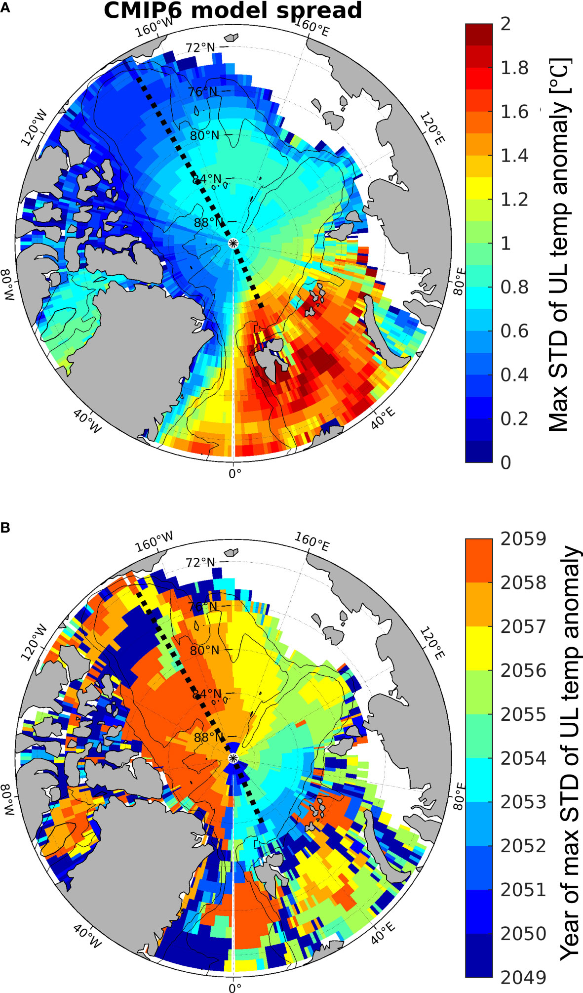
Figure 13 By mapping the model spread (standard deviation; STD) of the models, we attempt to better understand the source of the large spread. We here show (A) Maximum STD over the period 1993-2058 for the temperature anomaly in the Upper Layer (UL), based on the ssp126 scenario. The anomalies are calculated by subtracting the mean conditions in 1993-2010. The 500m and 2000m isobaths are shown (thin black curves) together with the position of the CAATEX section. (B) The year of the maximum STD. Note that the last colour (dark orange) means years equal to 2058 or higher.

The large model spread is related to the large CMIP5/6 model biases in the Arctic Ocean, which have been known for some time (Khosravi et al., 2022). Higher resolution ocean models and better parameterization of mixing can reduce such biases (e.g. Khosravi et al., 2022; Heuzé et al., 2023), but new biases are also found in the ocean due to biases in the atmospheric circulation above the Arctic Ocean (Hinrichs et al., 2021). Improvement of coupled global climate models will take time, and thus, we need to find additional ways of reducing the uncertainty of Arctic future trends, as we have alluded to in this study.

5 Summary and conclusions

We have systematically compared 13 CMIP6 model simulations against an ocean reanalysis product in the Central Arctic Ocean for the period 1993-2010. We have focused on how the models represent observed horizontal patterns of temperature and salinity in the Upper Layer (100-300m) and the Mid Layer (300-700m). We have found that only a few models represent these patterns relatively well. We consider it important that these large-scale patterns are represented in the models, to have confidence in the future scenarios for the Arctic Ocean.

In the ssp126 and ssp585 scenario, we have found that there is a large increase in the model spread for the projected temperature change in the CAATEX section (a section across the Central Arctic Ocean) in both layers. There is a steep change in the period from 2020-2040 from a standard deviation of 0.1°C in 2020 to about 0.5°C in 2040, which is a considerable increase. In the end of the 2050s, it has reached a level of about 0.6°C. Concentrating only on the models with good performance and their projections for the years 2045-2055 (MPI-ESM1-2-HR, IPSL-CM6A-LR, CESM2-WACCM, MRI-ESM2-0), they agree on a larger warming in the eastern part of the Central Arctic Ocean (east of the CAATEX section) compared to the western part, but the location of the maximum warming differs among the models.

With increasing CO2 levels and continued global warming, the Arctic Ocean shows at the end of this century a larger warming than what is projected for the global ocean (Shu et al., 2022). Such warming will have huge consequences on the marine life, sea ice, and societies in the Arctic region. However, as shown herein the spread in the warming among individual climate models is considerable. The main source of the spread on these time scales comes from model differences and not internal variability, as shown here and in other studies (e.g. Shu et al., 2022). This tells that caution is important when it comes to using these projected temperatures and salinities in the Central Arctic Ocean, and we need to find ways to reduce the uncertainty of the future projections.

Considering several metrics (e.g., our own pattern correlation, climate sensitivity, ocean heat transport), in addition to a comparison with other recent CMIP6 studies in the Arctic Ocean, we find that two of the models have an overall better performance (MPI-ESM1-2-HR, IPSL-CM6A-LR). Considering projected changes for temperature for the period 2045-2055 in the high end ssp585 scenario, they show a more similar warming in the Mid Layer (1.1-1.5°C). However, in the low end ssp126 scenario, IPSL-CM6A-LR shows a considerably higher warming than MPI-ESM1-2-HR. In contrast to the projected warming by both models, the projected salinity changes for the period 2045-2055 are very different; MPI-ESM1-2-HR shows a freshening in the Upper Layer, whereas IPSL-CM6A-LR shows a salinification in this layer.

Data availability statement

The original contributions presented in the study are included in the article/Supplementary Material. Further inquiries can be directed to the corresponding author.

Author contributions

HL designed the study and led the analysis and writing. HS contributed to the design of the study. AS contributed with results from the cruise data. PU and LR contributed with results from the ocean reanalysis data. All authors contributed to the discussion of the results and to the writing of the manuscript. All authors contributed to the article and approved the submitted version.

Funding

The research leading to these results has received funding from CAATEX (grant No. 280531) supported by the Research Council of Norway (RCN). In addition, this study is supported by the project MAPARC with grant No. 328943, funded by RCN. PU was supported by the European Union’s Horizon 2020 research and innovation framework programme (PolarRES project, grant No. 101003590). SO has received funding from The National Centre for Climate Research, hosted at the Danish Meteorological Institute. This publication is also part of the IS-ENES3 project that has received funding from the European Union’s Horizon 2020 research and innovation programme under grant agreement No. 824084.

Acknowledgments

We acknowledge the World Climate Research Programme, which, through its Working Group on Coupled Modelling, coordinated and promoted CMIP6. We thank the climate modeling groups for producing and making available their model output, the Earth System Grid Federation (ESGF) for archiving the data and providing access, and the multiple funding agencies who support CMIP6 and ESGF. We also thank Morven Muilwijk and the reviewers for their helpful and constructive comments that improved the manuscript significantly.

Conflict of interest

The authors declare that the research was conducted in the absence of any commercial or financial relationships that could be construed as a potential conflict of interest.

Publisher’s note

All claims expressed in this article are solely those of the authors and do not necessarily represent those of their affiliated organizations, or those of the publisher, the editors and the reviewers. Any product that may be evaluated in this article, or claim that may be made by its manufacturer, is not guaranteed or endorsed by the publisher.

Supplementary material

The Supplementary Material for this article can be found online at: https://www.frontiersin.org/articles/10.3389/fmars.2023.1211562/full#supplementary-material

References

Årthun M., Onarheim I. H., Dörr J., Eldevik T. (2021). The seasonal and regional transition to an ice-free arctic. Geophy. Res. Lett. 48, e2020GL090825. doi: 10.1029/2020GL090825

CrossRef Full Text | Google Scholar

Balmaseda M., Hernandez F., Storto A., Palmer M., Alves O., Shi L., et al. (2015). The ocean reanalyses intercomparison project (ora-ip). J. Operational Oceanogr. 8, s80–s97. doi: 10.1080/1755876X.2015.1022329

CrossRef Full Text | Google Scholar

Carmack E., Polyakov I., Padman L., Fer I., Hunke E., Hutchings J., et al. (2015). Toward quantifying the increasing role of oceanic heat in sea ice loss in the new arctic. Bull. Am. Meteorological Soc. 96, 2079–2105. doi: 10.1175/BAMS-D-13-00177.1

CrossRef Full Text | Google Scholar

Carmack E. C., Yamamoto-Kawai M., Haine T. W. N., Bacon S., Bluhm B. A., Lique C., et al. (2016). Freshwater and its role in the arctic marine system: Sources, disposition, storage, export, and physical and biogeochemical consequences in the arctic and global oceans. J. Geophy. Res.: Biogeosciences 121, 675–717. doi: 10.1002/2015JG003140

CrossRef Full Text | Google Scholar

Carton J. A., Giese B. S. (2008). A reanalysis of ocean climate using simple ocean data assimilation (soda). Monthly Weather Rev. 136, 2999–3017. doi: 10.1175/2007MWR1978.1

CrossRef Full Text | Google Scholar

Danabasoglu G., Lamarque J.-F., Bacmeister J., Bailey D. A., DuVivier A. K., Edwards J., et al. (2020). The community earth system model version 2 (cesm2). J. Adv. Modeling Earth Syst. 12, e2019MS001916s. doi: 10.1029/2019MS001916

CrossRef Full Text | Google Scholar

Docquier D., Grist J. P., Roberts M. J., Roberts C. D., Semmler T., Ponsoni L., et al. (2019). Impact of model resolution on arctic sea ice and north atlantic ocean heat transport. Climate Dynamics 53, 4989–5017. doi: 10.1007/s00382-019-04840-y

CrossRef Full Text | Google Scholar

Docquier D., Koenigk T. (2021). Observation-based selection of climate models projects arctic ice-free summers around 2035. Commun. Earth Environ. 2, 144. doi: 10.1038/s43247-021-00214-7

CrossRef Full Text | Google Scholar

Döscher R., Acosta M., Alessandri A., Anthoni P., Arsouze T., Bergman T., et al. (2022). The ec-earth3 earth system model for the coupled model intercomparison project 6. Geoscientific Model. Dev. 15, 2973–3020. doi: 10.5194/gmd-15-2973-2022

CrossRef Full Text | Google Scholar

Dunne J. P., Horowitz L. W., Adcroft A. J., Ginoux P., Held I. M., John J. G., et al. (2020). The gfdl earth system model version 4.1 (gfdl-esm 4.1): Overall coupled model description and simulation characteristics. J. Adv. Modeling Earth Syst. 12, e2019MS002015. doi: 10.1029/2019MS002015

CrossRef Full Text | Google Scholar

Good S. A., Martin M. J., Rayner N. A. (2013). En4: Quality controlled ocean temperature and salinity profiles and monthly objective analyses with uncertainty estimates. J. Geophy. Res.: Oceans 118, 6704–6716. doi: 10.1002/2013JC009067

CrossRef Full Text | Google Scholar

Heuzé C. (2021). Antarctic bottom water and north atlantic deep water in cmip6 models. Ocean Sci. 17, 59–90. doi: 10.5194/os-17-59-2021

CrossRef Full Text | Google Scholar

Heuzé C., Zanowski H., Karam S., Muilwijk M. (2023). The deep arctic ocean and fram strait in cmip6 models. J. Climate 36, 2551–2584. doi: 10.1175/JCLI-D-22-0194.1

CrossRef Full Text | Google Scholar

Hinrichs C., Wang Q., Koldunov N., Mu L., Semmler T., Sidorenko D., et al. (2021). Atmospheric wind biases: A challenge for simulating the arctic ocean in coupled models? J. Geophy. Res.: Oceans 126, e2021JC017565. doi: 10.1029/2021JC017565

CrossRef Full Text | Google Scholar

Holloway G., Dupont F., Golubeva E., Häkkinen S., Hunke E., Jin M., et al. (2007). Water properties and circulation in arctic ocean models. J. Geophys. Res.: Oceans 112, C04S03. doi: 10.1029/2006JC003642

CrossRef Full Text | Google Scholar

Huang B., Wang Z., Yin X., Arguez A., Graham G., Liu C., et al. (2021). Prolonged marine heatwaves in the arctic: 1982-2020. Geophy. Res. Lett. 48, e2021GL095590. doi: 10.1029/2021GL095590

CrossRef Full Text | Google Scholar

Ilıcak M., Drange H., Wang Q., Gerdes R., Aksenov Y., Bailey D., et al. (2016). An assessment of the arctic ocean in a suite of interannual core-ii simulations. part iii: Hydrography and fluxes. Ocean Model. 100, 141–161. doi: 10.1016/j.ocemod.2016.02.004

CrossRef Full Text | Google Scholar

IPCC (2021). Climate Change 2021: The Physical Science Basis. Contribution of Working Group I to the Sixth Assessment Report of the Intergovernmental Panel on Climate Change. Eds. Masson-Delmotte V., Zhai P., Pirani A., Connors S. L., Péan C., Berger S., Caud N., Chen Y., Goldfarb L., Gomis M. I., Huang M., Leitzell K., Lonnoy E., Matthews J. B. R., Maycock T. K., Waterfield T., Yelekçi O., Yu R., Zhou B. (Cambridge, United Kingdom and New York, NY, USA: Cambridge University Press).

Google Scholar

Khosravi N., Wang Q., Koldunov N., Hinrichs C., Semmler T., Danilov S., et al. (2022). The arctic ocean in cmip6 models: Biases and projected changes in temperature and salinity. Earth’s Future 10, e2021EF002282. doi: 10.1029/2021EF002282

CrossRef Full Text | Google Scholar

Langehaug H. R., Ortega P., Counillon F., Matei D., Maroon E., Keenlyside N., et al. (2022). Propagation of thermohaline anomalies and their predictive potential along the atlantic water pathway. J. Climate 35, 2111–2131. doi: 10.1175/JCLI-D-20-1007.1

CrossRef Full Text | Google Scholar

Lin Y., Huang X., Liang Y., Qin Y., Xu S., Huang W., et al. (2020). Community integrated earth system model (ciesm): Description and evaluation. J. Adv. Modeling Earth Syst. 12, e2019MS002036. doi: 10.1029/2019MS002036

CrossRef Full Text | Google Scholar

Lique C. (2015). Arctic sea ice heated from below. Nat. Geosci. 8, 172–173. doi: 10.1038/ngeo2357

CrossRef Full Text | Google Scholar

Locarnini R. A., Mishonov A. V., Antonov J. I., Boyer T. P., Garcia H. E., Baranova O. K., et al. (2013). World ocean atlas 2013, Volume 1: temperature. Eds. Levitus S., Mishonov A. (Technical. NOAA Atlas NESDIS). 73, 40. doi: 10.7289/V55X26VD

CrossRef Full Text | Google Scholar

Lurton T., Balkanski Y., Bastrikov V., Bekki S., Bopp L., Braconnot P., et al. (2020). Implementation of the cmip6 forcing data in the ipsl-cm6a-lr model. J. Adv. Modeling Earth Syst. 12, e2019MS001940. doi: 10.1029/2019MS001940

CrossRef Full Text | Google Scholar

Madonna E., Sandø A. B. (2022). Understanding differences in north atlantic poleward ocean heat transport and its variability in global climate models. Geophy. Res. Lett. 49, e2021GL096683. doi: 10.1029/2021GL096683

CrossRef Full Text | Google Scholar

Mauritsen T., Bader J., Becker T., Behrens J., Bittner M., Brokopf R., et al. (2019). Developments in the mpi-m earth system model version 1.2 (mpi-esm1.2) and its response to increasing co2. J. Adv. Modeling Earth Syst. 11, 998–1038. doi: 10.1029/2018MS001400

CrossRef Full Text | Google Scholar

Meehl G. A., Senior C. A., Eyring V., Flato G., Lamarque J.-F., Stouffer R. J., et al. (2020). Context for interpreting equilibrium climate sensitivity and transient climate response from the cmip6 earth system models. Sci. Adv. 6, eaba1981. doi: 10.1126/sciadv.aba1981

PubMed Abstract | CrossRef Full Text | Google Scholar

Meinshausen M., Nicholls Z. R. J., Lewis J., Gidden M. J., Vogel E., Freund M., et al. (2020). The shared socio-economic pathway (ssp) greenhouse gas concentrations and their extensions to 2500. Geoscientific Model. Dev. 13, 3571–3605. doi: 10.5194/gmd-13-3571-2020

CrossRef Full Text | Google Scholar

Mohamed B., Nilsen F., Skogseth R. (2022). Marine heatwaves characteristics in the barents sea based on high resolution satellite data, (1982–2020). Front. Mar. Sci. 9. doi: 10.3389/fmars

PubMed Abstract | CrossRef Full Text | Google Scholar

Muilwijk M., Nummelin A., Heuze,´ C., Polyakov I. V., Zanowski H., Smedsrud L. H. (2023). Divergence in climate model projections of future arctic atlantification. J. Climate 36, 1727–1748. doi: 10.1175/JCLI-D-22-0349.1

CrossRef Full Text | Google Scholar

Müller W. A., Jungclaus J. H., Mauritsen T., Baehr J., Bittner M., Budich R., et al. (2018). A higher-resolution version of the max planck institute earth system model (mpi-esm1.2-hr). J. Adv. Modeling Earth Syst. 10, 1383–1413. doi: 10.1029/2017MS001217

CrossRef Full Text | Google Scholar

Notz D., SIMIP Community. (2020). Arctic sea ice in cmip6. Geophys. Res. Lett. 47, e2019GL086749. doi: 10.1029/2019GL086749

CrossRef Full Text | Google Scholar

O’Neill B. C., Tebaldi C., van Vuuren D. P., Eyring V., Friedlingstein P., Hurtt G., et al. (2016). The scenario model intercomparison project (scenariomip) for cmip6. Geoscientific Model. Dev. 9, 3461–3482. doi: 10.5194/gmd-9-3461-2016

CrossRef Full Text | Google Scholar

Pan R., Shu Q., Wang Q., Wang S., Song Z., He Y., et al. (2023). Future arctic climate change in cmip6 strikingly intensified by nemo-family climate models. Geophys. Res. Lett. 50, e2022GL102077. doi: 10.1029/2022GL102077

CrossRef Full Text | Google Scholar

Polyakov I. V., Alkire M. B., Bluhm B. A., Brown K. A., Carmack E. C., Chierici M., et al. (2020). Borealization of the arctic ocean in response to anomalous advection from sub-arctic seas. Front. Mar. Sci. 7. doi: 10.3389/fmars.2020.00491

CrossRef Full Text | Google Scholar

Rantanen M., Karpechko A. Y., Lipponen A., Nordling K., Hyvarinen,¨ O., Ruosteenoja K., et al. (2022). The arctic has warmed nearly four times faster than the globe since 1979. Commun. Earth Environ. 3, 168. doi: 10.1038/s43247-022-00498-3

CrossRef Full Text | Google Scholar

Rautiainen L. (2020). Observed Changes in the Hydrography of the Arctic Ocean. Helsinki, Finland: University of Helsinki. Available at: http://hdl.handle.net/10138/313591.

Google Scholar

Richards A. E., Johnson H. L., Lique C. (2022). Spatial and temporal variability of atlantic water in the arctic from 40 years of observations. J. Geophy. Res.: Oceans 127, e2021JC018358. doi: 10.1029/2021JC018358

CrossRef Full Text | Google Scholar

Rong X.-Y., Li J., Chen H.-M., Xin Y.-F., Su J.-Z., Hua L.-J., et al. (2019). Introduction of cams-csm model and its participation in cmip6. Adv. Climate Change Res. 15, 540–544. doi: 10.12006/j.issn.1673-1719.2019.186

CrossRef Full Text | Google Scholar

Rudels B., Friedrich H. J., Quadfasel D. (1999). The arctic circumpolar boundary current. Deep Sea Res. Part II: Topical Stud. Oceanogr. 46, 1023–1062. doi: 10.1016/S0967-0645(99)00015-6

CrossRef Full Text | Google Scholar

Sandø A. B., Gao Y., Langehaug H. R. (2014). Poleward ocean heat transports, sea ice processes, and arctic sea ice variability in noresm1-m simulations. J. Geophy. Res.: Oceans 119, 2095–2108. doi: 10.1002/2013JC009435

CrossRef Full Text | Google Scholar

Séférian R., Nabat P., Michou M., Saint-Martin D., Voldoire A., Colin J., et al. (2019). Evaluation of cnrm earth system model, cnrm-esm2-1: Role of earth system processes in present-day and future climate. J. Adv. Modeling Earth Syst. 11, 4182–4227. doi: 10.1029/2019MS001791

CrossRef Full Text | Google Scholar

Seland Ø., Bentsen M., Olivié D., Toniazzo T., Gjermundsen A., Graff L. S., et al. (2020). Overview of the norwegian earth system model (noresm2) and key climate response of cmip6 deck, historical, and scenario simulations. Geoscientific Model. Dev. 13, 6165–6200. doi: 10.5194/gmd-13-6165-2020

CrossRef Full Text | Google Scholar

Shu Q., Wang Q., Årthun M., Wang S., Song Z., Zhang M., et al. (2022). Arctic ocean amplification in a warming climate in cmip6 models. Sci. Adv. 8, eabn9755. doi: 10.1126/sciadv.abn9755

PubMed Abstract | CrossRef Full Text | Google Scholar

Shu Q., Wang Q., Su J., Li X., Qiao F. (2019). Assessment of the atlantic water layer in the arctic ocean in cmip5 climate models. Climate Dynamics 53, 5279–5291. doi: 10.1007/s00382-019-04870-6

CrossRef Full Text | Google Scholar

Smedsrud L. H., Muilwijk M., Brakstad A., Madonna E., Lauvset S. K., Spensberger C., et al. (2022). Nordic seas heat loss, atlantic inflow, and arctic sea ice cover over the last century. Rev. Geophysics 60, e2020RG000725. doi: 10.1029/2020RG000725

CrossRef Full Text | Google Scholar

Stallemo A. (2022). Upper-ocean hydrography in the Eurasian Basin and its implication on sound speed. Bergen, Norway: University of Bergen. Available at: https://hdl.handle.net/11250/3014836.

Google Scholar

Storto A., Masina S., Navarra A. (2016). Evaluation of the cmcc eddy-permitting global ocean physical reanalysis system (c-glors 1982–2012) and its assimilation components. Q. J. R. Meteorological Soc. 142, 738–758. doi: 10.1002/qj.2673

CrossRef Full Text | Google Scholar

Sumata H., Kauker F., Karcher M., Rabe B., Timmermans M.-L., Behrendt A., et al. (2018). Decorrelation scales for arctic ocean hydrography – part i: Amerasian basin. Ocean Sci. 14, 161–185. doi: 10.5194/os-14-161-2018

CrossRef Full Text | Google Scholar

Swart N. C., Cole J. N. S., Kharin V. V., Lazare M., Scinocca J. F., Gillett N. P., et al. (2019). The canadian earth system model version 5 (canesm5.0.3). Geoscientific Model. Dev. 12, 4823–4873. doi: 10.5194/gmd-12-4823-2019

CrossRef Full Text | Google Scholar

Tietsche S., Balmaseda M. A., Zuo H., Mogensen K. (2017). Arctic sea ice in the global eddypermitting ocean reanalysis orap5. Climate Dynamics 49, 775–789. doi: 10.1007/s00382-015-2673-3

CrossRef Full Text | Google Scholar

Timmermans M.-L., Marshall J. (2020). Understanding arctic ocean circulation: A review of ocean dynamics in a changing climate. J. Geophy. Res.: Oceans 125, e2018JC014378. doi: 10.1029/2018JC014378

CrossRef Full Text | Google Scholar

Timmermans M.-L., Toole J., Krishfield R. (2018). Warming of the interior arctic ocean linked to sea ice losses at the basin margins. Sci. Adv. 4, eaat6773. doi: 10.1126/sciadv.aat6773

PubMed Abstract | CrossRef Full Text | Google Scholar

Tokarska K. B., Stolpe M. B., Sippel S., Fischer E. M., Smith C. J., Lehner F., et al. (2020). Past warming trend constrains future warming in cmip6 models. Sci. Adv. 6, eaaz9549. doi: 10.1126/sciadv.aaz9549

PubMed Abstract | CrossRef Full Text | Google Scholar

Toyoda T., Fujii Y., Yasuda T., Usui N., Ogawa K., Kuragano T., et al. (2016). Data assimilation of sea ice concentration into a global ocean–sea ice model with corrections for atmospheric forcing and ocean temperature fields. J. Oceanogr. 72, 235–262. doi: 10.1007/s10872-015-0326-0

CrossRef Full Text | Google Scholar

Uotila P., Goosse H., Haines K., Chevallier M., Barthélemy A., Bricaud C., et al. (2019). An assessment of ten ocean reanalyses in the polar regions. Climate Dynamics 52, 1613–1650. doi: 10.1007/s00382-018-4242-z

CrossRef Full Text | Google Scholar

Valdivieso M., Haines K., Zuo H., Lea D. (2014). Freshwater and heat transports from global ocean synthesis. J. Geophy. Res.: Oceans 119, 394–409. doi: 10.1002/2013JC009357

CrossRef Full Text | Google Scholar

Volodin E., Gritsun A. (2018). Simulation of observed climate changes in 1850–2014 with climate model inm-cm5. Earth System Dynamics 9, 1235–1242. doi: 10.5194/esd-9-1235-2018

CrossRef Full Text | Google Scholar

Wienrich N., Buschman V. Q., Coon C., Fuller S., Hennicke J., Humrich C., et al. (2022). The ecosystem approach to marine management in the arctic: Opportunities and challenges for integration. Front. Mar. Sci. 9. doi: 10.3389/fmars.2022.1034510

PubMed Abstract | CrossRef Full Text | Google Scholar

Worcester P. F., Dzieciuch M. A., Sagen H. (2020). Ocean acoustics in the rapidly changing Arctic. Acoustics Today 16 (1), 55–63. doi: 10.1121/AT.2020.16.1.55

CrossRef Full Text | Google Scholar

Yukimoto S., Kawai H., Koshiro T., Oshima N., Yoshida K., Urakawa S., et al. (2019). The meteorological research institute earth system model version 2.0, mri-esm2.0: Description and basic evaluation of the physical component. J. Meteorological Soc. Japan. Ser. II 97, 931–965. doi: 10.2151/jmsj.2019-051

CrossRef Full Text | Google Scholar

Zanowski H., Jahn A., Holland M. M. (2021). Arctic ocean freshwater in cmip6 ensembles: Declining sea ice, increasing ocean storage and export. J. Geophy. Res.: Oceans 126, e2020JC016930. doi: 10.1029/2020JC016930

CrossRef Full Text | Google Scholar

Zuo H., Balmaseda M. A., Mogensen K. (2017). The new eddy-permitting orap5 ocean reanalysis: description, evaluation and uncertainties in climate signals. Climate Dynamics 49, 791–811. doi: 10.1007/s00382-015-2675-1

CrossRef Full Text | Google Scholar

Zuo H., Balmaseda M. A., Tietsche S., Mogensen K., Mayer M. (2019). The ecmwf operational ensemble reanalysis–analysis system for ocean and sea ice: a description of the system and assessment. Ocean Sci. 15, 779–808. doi: 10.5194/os-15-779-2019

CrossRef Full Text | Google Scholar

Zweng M. M., Reagan J. R., Antonov J. I., Locarnini R. A., Mishonov A. V., Boyer T. P., et al. (2013). World ocean atlas 2013, Volume 2: salinity. Eds. Levitus S., Mishonov A. Technical. (NOAA Atlas NESDIS). 74, 39.

Google Scholar