KRILLPODYM: a mechanistic, spatially resolved model of Antarctic krill distribution and abundance

1 Introduction

The interplay between species life history and environmental spatio-temporal processes is fundamental in determining population connectivity (Levin, 1992). This plays a crucial role in informing effective species management (Treml et al., 2008; Rassweiler et al., 2020), particularly in the face of global change (Carr et al., 2017). Prediction of how populations might respond to environmental change requires the interfacing of factors controlling individual growth, survival, and reproduction, with processes affecting distribution. This is especially true for polar marine species, such as Antarctic krill Euphausia superba, which are strongly influenced by the extreme seasonality of environmental conditions (Hagen and Auel, 2001; Kawaguchi et al., 2007).

Antarctic krill (hereafter krill) have a complex life history with numerous developmental stages that each depend on a unique suite of biophysical conditions to grow and survive (Thorpe et al., 2019). This complex history leads to a strong bottom-up control of the population (Hofmann and Hüsrevoğlu, 2003; Loeb et al., 2009). For example, primary productivity over spring and summer determines the timing and magnitude of spawning, and the growth of recently spawned larvae (Ross and Quetin, 1989), while recruitment is dependent on the spatial extent of winter sea-ice (Kawaguchi and Satake, 1994; Wiedenmann et al., 2009). These dependencies make krill potentially susceptible to changing biophysical conditions. Indeed, in recent decades krill’s range has contracted southwards in the face of warming and reductions in sea-ice extent, with concomitant increases in population mean length (population aging) arising from poor recruitment (Atkinson et al., 2019, but see also Cox et al., 2018; Candy, 2021). These changes are particularly concerning both because of its importance within Southern Ocean food webs (Murphy et al., 2007; Saunders et al., 2019; McCormack et al., 2020), and because it is commercially harvested. Currently, krill fishing occurs only within the Southwest Atlantic, but while landings remain well below the total annual catch limit (8.6 million tons; Nicol et al., 2012) set by the Commission for the Conservation of Antarctic Marine Living Resources (CCAMLR), there are growing concerns over the increasingly localised nature of this fishery and its impacts on dependent ecosystems (Lowther et al., 2020; Krüger et al., 2021). Under these combined pressures there is increasing need for spatio-temporally resolved frameworks that capture the dynamics and environmental underpinnings of the krill population, building capacity for fine-scale management of the species (e.g. Constable and Nicol, 2002).

While there is growing understanding of the relationships between biophysical conditions and krill life history requirements (e.g. Siegel and Watkins, 2016), there remains limited representation of the transport processes that control krill’s distribution within these environments (Meyer et al., 2020). Yet, to project krill responses to change, spatial population processes need to be modelled across multiple generations and with a circumpolar range. To date, much of the work considering krill transport has used particle tracking (Lagrangian) techniques (e.g. Fach and Klinck, 2006; Mori et al., 2019; Veytia et al., 2021), which become very computationally expensive (Jones et al., 2016) when considering a full life cycle and large spatial scales. Eulerian approaches offer a computationally efficient alternative, by computing spatial dynamics on a gridded density field using advection-diffusion-reaction equations. This is already commonplace in ocean circulation modelling, but efforts in recent decades to integrate this methodology with population modelling have generated capacity for extending the approach to pelagic organisms (Lehodey et al., 2008; Maury, 2010).

The Spatial Ecosystem And Population Dynamics Model (SEAPODYM) is one such framework. SEAPODYM couples general circulation and biogeochemical forcings with mechanistic bioenergetic functions to simulate the spatial and temporal fluxes of pelagic ocean biomass across multiple trophic levels (Lehodey et al., 2008; Senina et al., 2008; Lehodey et al., 2010; Lehodey et al., 2015; Senina et al., 2020). To achieve this, the model makes use of two component sub-models. The first sub-model uses bioenergetics to simulate the spatial dynamics of mid-trophic level organisms (micronekton), represented as 6 functional groups occurring across three broad pelagic depth zones (epipelagic, upper mesopelagic and lower mesopelagic, with the width of each being defined as multiples of euphotic depth; Lehodey et al., 2015). The second sub-model extends the first by incorporating a population model to represent the spatial dynamics of key predatory (fish) species feeding on mid-trophics. Initially, this population model focused on tuna species (Lehodey, 2004) but has since been generalised to other tuna-like predators (Abecassis et al., 2011; Dragon et al., 2018) as well as small pelagic fish (Hernandez et al., 2014). The approach allows SEAPODYM to jointly consider life history, as well as transport processes acting to reshape distribution and interactions with the biophysical environment. This gives the model considerable flexibility to be adapted for other pelagic species with complex life histories, such as krill.

Here, we present a framework and first implementation adapting the predator sub-model of SEAPODYM to create a new model – KRILLPODYM. This model is specifically modified to simulate the spatio-temporal dynamics of krill within the circumpolar Southern Ocean. Below, we detail the new model in terms of the three major structural components required to achieve a krill-centred version of SEAPODYM, namely:

1. an age-structured population reflecting the life history of krill, together with population-level processes including age-dependent growth and survival

2. key habitat requirements affecting spawning and modulating krill survival at different ages

3. major transport processes acting to redistribute krill biomass depending on its vertical position within the water column

Following this, we provide output from the initialisation and first simulation of KRILLPODYM and discuss potential applications, noting that fisheries and fishing impact are to be included at a later stage of development.

2 Methods

2.1 Framework for the three integrated structural components of KRILLPODYM

2.1.1 Component 1: considering an age-structured population with growth, survival, and reproduction

2.1.1.1 Age structure

Antarctic krill have a complex life-history in which they transition through 13 larval stages, and a juvenile stage (Ikeda, 1984; Kawaguchi, 2016), before reaching maturity (adult). For modelling purposes, these 15 developmental stages can be allocated amongst five broader life stages, based on unique physiological requirements and how they interact with the environment.

Model stage 1 – The first life stage (young larvae; Figure 1) occurs during the descent/ascent cycle and lasts about one month (Ikeda, 1984; Hofmann et al., 1992). Krill eggs sink to depths of 500-1000 m (Hofmann et al., 1992) before hatching as yolk-dependent larvae and subsequently returning to the surface. Over this period, krill likely experience different transport conditions from later stages, which are later largely associated with the upper 200m of the water column (e.g. Godlewska and Klusek, 1987; Bestley et al., 2018).

FIGURE 1

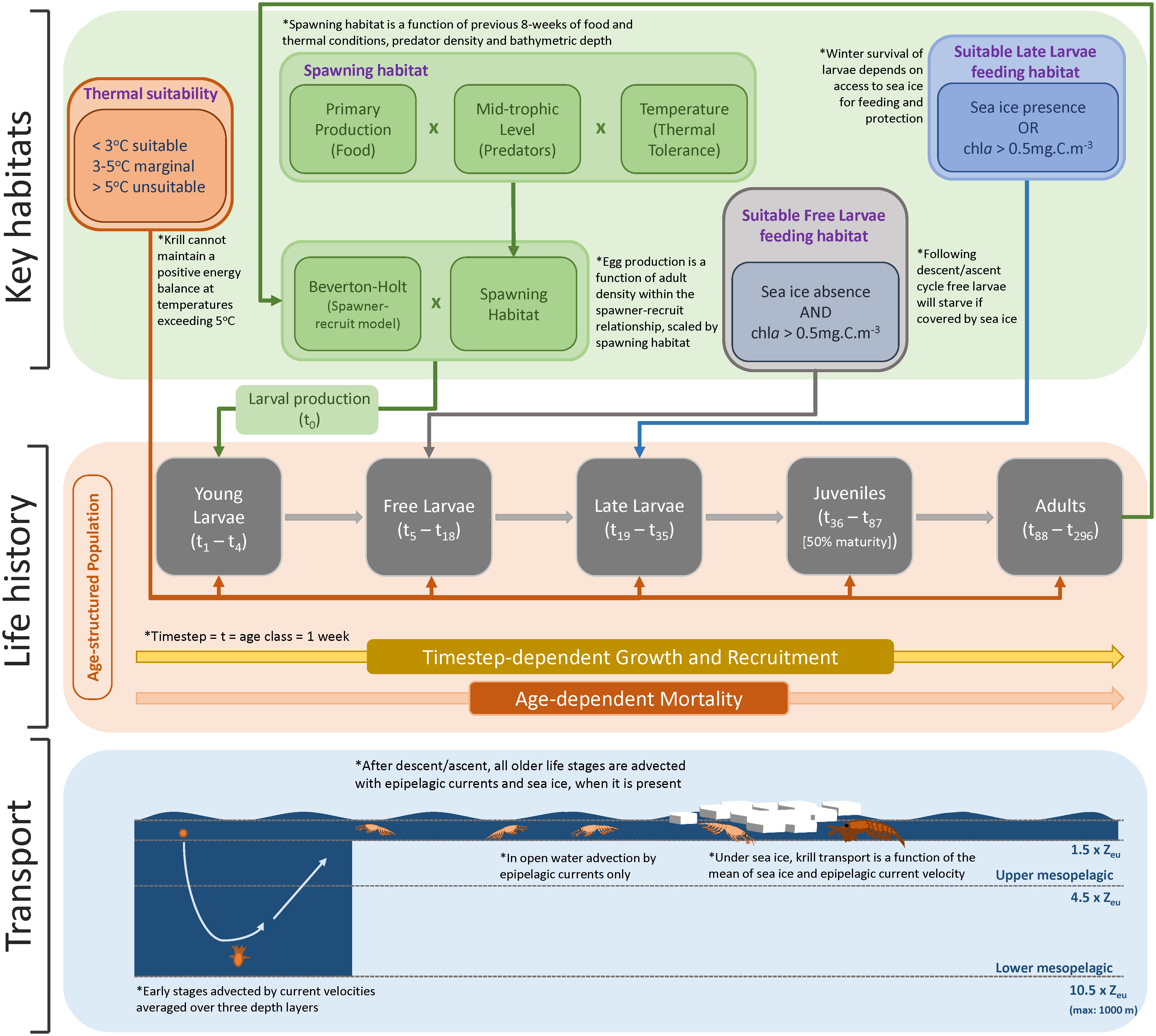
Figure 1 Conceptualisation of KRILLPODYM highlighting the three major structural components within the model, namely: 1) age-structured population with distinct life stages, each consisting of multiple age classes lasting the time step of the model (1 week); 2) key habitat requirements, including thermal requirements across all life stages, spawning habitat which, together with a stock-recruit model, modulates the number of larvae introduced into the system by mature adults, open water requirements for free larvae, and sea ice presence for late larvae that must survive winter in order to recruit; and 3) transport of krill based on associated life stage, including transport with average current velocities across the full mesopelagic water column for young larvae undergoing the descent/ascent cycle, and current or current and ice driven transport, based on the presence of sea ice for all older life stages.

Model stage 2 – Upon reaching the surface, larvae transition into the next life stage (stage 2 – free larvae; Figure 1). Free larvae (calyptopes) have generally exhausted their yolk reserves, and have limited fasting capacity, so must begin feeding immediately (Ross and Quetin, 1989). Feeding during this stage requires access to ice-free waters and phytoplankton as these krill lack thoracic appendages necessary for feeding on ice algae (Jia et al., 2014).

Model stage 3 – After approximately three months (Ikeda, 1984; Hofmann et al., 1992), coinciding with the autumn advance of sea ice, summer-spawned krill transition into furcilia IV or higher larval stages (stage 3 – late larvae; Figure 1), which, like post-larval krill, are able to swarm and have fully developed feeding baskets for grazing on ice algae (Jia et al., 2014). Larval krill that successfully recruit into the juvenile population likely overwinter at this developmental stage (Daly, 2004), during which they are thought to feed on sea ice algae as a dominant food source.

Model stage 4 – Recruitment into the juvenile (stage 4; Figure 1) population occurs in the spring a year after spawning.

Model stage 5 – Half of the juvenile population later mature as adult (stage 5; Figure 1) female krill (age at 50% maturity) at the end of their second winter (Siegel and Loeb, 1994), while the remaining juveniles recruit as adult males a year later. For female krill spawned in January – the prevalent month of spawning (Hosie et al., 1988; Spiridonov, 1995; Siegel, 2012; Kawaguchi, 2016) – this would coincide with an age of approximately 88 weeks. Male krill subsequently mature after the third winter (Siegel and Loeb, 1994)

Following the same structural approach as SEAPODYM, we formalise these generalised life history requirements into an age-structured population that comprises a total of 291 age classes, each lasting one week, and covering the full life span (~ 6 years) (Table 1). Age classes are allocated amongst the five broad life stages described above and each has its own unique length, weight, and survival (as determined by age; see below Age-dependent growth and Age-dependent mortality for details) (Figure 1). The last age class (week 291) also contains any remaining krill that are older than this (Table 1). At any time, each age class has a given density of individuals allocated to it, the magnitude of which depends on recruitment from the previous (younger) age class.

TABLE 1

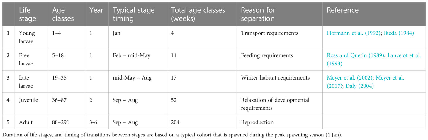
Table 1 Key life stages and their duration as defined by age classes, each lasting a week.

2.1.1.2 Age-dependent growth

Based on the age-structured population outlined above, growth between age classes is predetermined and dependent on time (Lehodey et al., 2008). To assign lengths to individual age classes we use a seasonal, stepwise von Bertalanffy growth curve (Figure 2) following methods used in Rosenberg et al. (1986), and which assumes an asymptotic maximum length of 60 mm, such that:

FIGURE 2

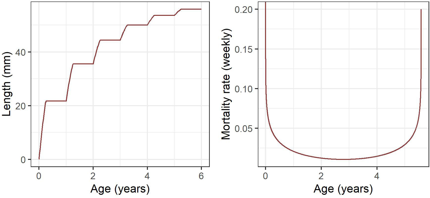
Figure 2 Seasonal, stepwise von Bertalanffy growth curve following Rosenberg et al. (1986) (left) and weekly age-dependent mortality following Pakhomov (1995a) (right) represented as a modified quadratic function with high mortality rates in early life and as krill approach 6 years old.

$\begin{array}{ll}\{\begin{array}{ll}{I}_t=L_{inf}(1-e^{-k(t-n(1-g))})\hfill & n<t\le n+g\hfill \\ I_t=I_{t+g}\hfill & n+g<t<n+1\hfill \end{array}& (1)\end{array}$

Where $I_t$ is length at time $t$ And $L_{inf}$ is asymptotic maximum length (mm). Seasonal growth is determined by a growth constant ($k$), proportion of the year when krill grow ($g$) and the number of winters survived ($n$).

While this model does not explicitly consider shrinkage (Candy and Kawaguchi, 2006; Constable and Kawaguchi, 2018), it provides a simple approximation of length-at-age by allowing for rapid growth in spring and summer, and zero growth over winter. Cohorts older than 6 years are all assigned to an adult+ age/size class which represents the maximum size and age of individual krill. Thereafter, we then assign a basic estimate of mass for each age-class based on its exponential relationship with length, following methods outlined in Ju and Harvey (2004), such that:

$\begin{array}{ll}WW=(0.1·{10}^{-6})·T{L}^{3.478}& (2)\end{array}$

Where $WW$ is wet weight ($g$) and TL denotes total length (length from anterior margin of the eye to the tip of the telson; mm).

2.1.1.3 Age-dependent mortality

Krill mortality is highly variable depending on age. Both empirical and model-based studies indicate that mortality is highest for the first and last years, declining at intermediate ages towards a minimum in adult krill of approximately three years age (Pakhomov, 1995b). High mortality in early life is likely driven by predation and starvation (Ryabov et al., 2017), with senescence playing a larger role in older individuals. We represent age-dependent mortality using the following equation (Figure 2) with parameter values taken from Pakhomov (1995a) such that:

$\begin{array}{ll}m(t)=\frac{(-1·log(1-(a·t^2+b·t+c)))}{52}& (3)\end{array}$

Where $t$ is age, while $a$ and $b$ denote the quadratic slope coefficients and $c$ the intercept of the estimated annual extinction rate respectively. The quadratic slope function is parameterised such that the extinction rate remains $\le$ 1, to ensure that the log in equation 3 remains defined for all age classes. The numerator represents annual mortality rates (Pakhomov, 1995b), and has been divided by 52 to give mortality rates at the weekly time step of this model.

2.1.2 Component 2: representing key habitat requirements modulating spawning and survival of different life stages

Numerous environmental variables control krill populations through their effects on spawning (Schmidt et al., 2012), growth (Murphy et al., 2017), and survival (Perry et al., 2020; Tarling, 2020). For example, studies addressing winter survival of larvae, make use of a combination of sea-ice variables (e.g. sea ice concentration, thickness and ridging rate) to provide better estimates of the 3-dimensional structure of under ice habitat (Melbourne-Thomas et al., 2016; Veytia et al., 2021) than simple metrics of areal ice coverage. However, for the whole-of-life-cycle approach adopted by this study, we follow a similar approach to Thorpe et al. (2019) and make use of relatively simple habitat rules based on variables known to have the strongest influence on krill throughout their life. In particular, ocean temperature, primary production, and the presence or absence of sea ice (see ESM Table S1 for specific variables used in habitat calculation, along with associated sources).

To do so, we define two habitat categories: one that considers the suitability of habitat for spawning, which scales the production of larvae, while a second modulates survival of the five life stages based on their specific physiological requirements.

2.1.2.1 Habitat category 1: spawning habitat and larval production

The magnitude of larval production is strongly influenced by the quality of the underlying environment (Marrari et al., 2008; Conroy et al., 2020), as well as the density of adult krill (Ryabov et al., 2017). We compute larval production as the product of spawning habitat quality and a stock-recruitment model representing the density ratio between adults and larvae. Spawning habitat quality is calculated as the product of biological suitability functions considering adult thermal and feeding conditions over the 8 weeks before spawning, as well as the density of micronekton (predators) at the time of spawning. Here, we provide an overview how spawning habitat is calculated, but the detailed implementation of this model can be found in Green et al. (2021).

We represent habitat quality as the product of suitability scores (scaled 0-1) for key biophysical variables that affect egg production and survival. This approach uses three key variables: (i) temperature; (ii) net primary productivity (PP); and (iii) predator density. Spawning habitat quality (Hs) can be defined as:

$\begin{array}{ll}{H}_s=f_1(T)·f_2(PP)·f_3(Pred)& (4)\end{array}$

where $f_1(T)$ denotes a sigmoid function (Eq.5.) representing metabolic tolerance of adult krill to variations in temperature, $f_2(PP)$ gives a Holling type III functional response (Eq.6.) representing the suitability of the feeding environment ($PP$) for egg production, and $f_3(Pred)$ is a modified lognormal function (Eq.7.) representing survival of eggs and larvae under predation.

$\begin{array}{ll}{f}_1(T)=\frac{1}{1+ ex{p}^{\lambda (T-\theta )}}& (5)\end{array}$

$\begin{array}{ll}{f}_2(PP)=\frac{P{P}^2}{\alpha + P{P}^2}& (6)\end{array}$

$\begin{array}{ll}{f}_3(Pred)=\frac{e^{\mu -0.5·{\sigma }^2-\frac{{(log(Pred+1)-\mu )}^2}{2·{\sigma }^2}}}{Pred+1}& (7)\end{array}$

Estimated spawning habitat quality is computed for each timestep and is combined with a Beverton-Holt model (Figure 3), to modify the stock-recruit relationship between adult density at a given location and the number of young larvae produced in the following timestep. The Beverton-Holt model is represented by equation 8 below, where Adults denotes adult krill density R represents the maximum reproductive rate, H_s inputs spawning habitat quality as calculated in eq. 4, and β is a slope coefficient that modulates density dependence (see also Figure 4. Initial parameter 201 values are given in Table 2. Krill spawn predominantly over austral summer (Kawaguchi, 2016). To represent this, we constrain krill spawning activity to occur only between 1 Dec and 28 Feb.

FIGURE 3

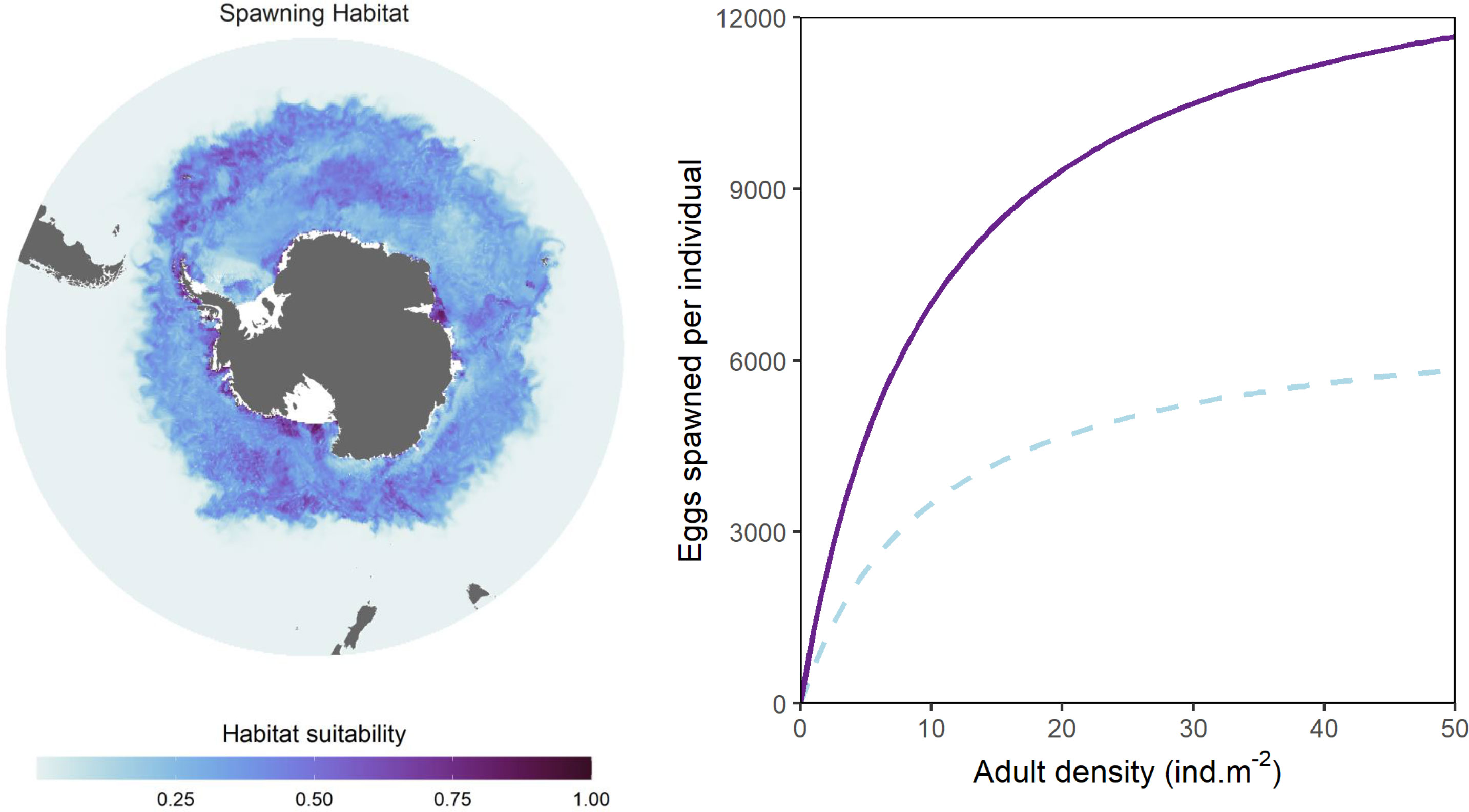
Figure 3 Illustration of modelled spawning habitat quality (left) and the Beverton-Holt stock-recruitment function used to modulate larval production (right). Spawning habitat quality is given for the first week of January (i.e. during peak spawning season) and follows Green et al. (2021). The two curves representing the Beverton-Holt function (right) denote the relationship between adult density and number of spawned eggs for spawning habitat values of 1 (high quality; solid purple line) and 0.5 (moderate quality; dashed blue line).

FIGURE 4

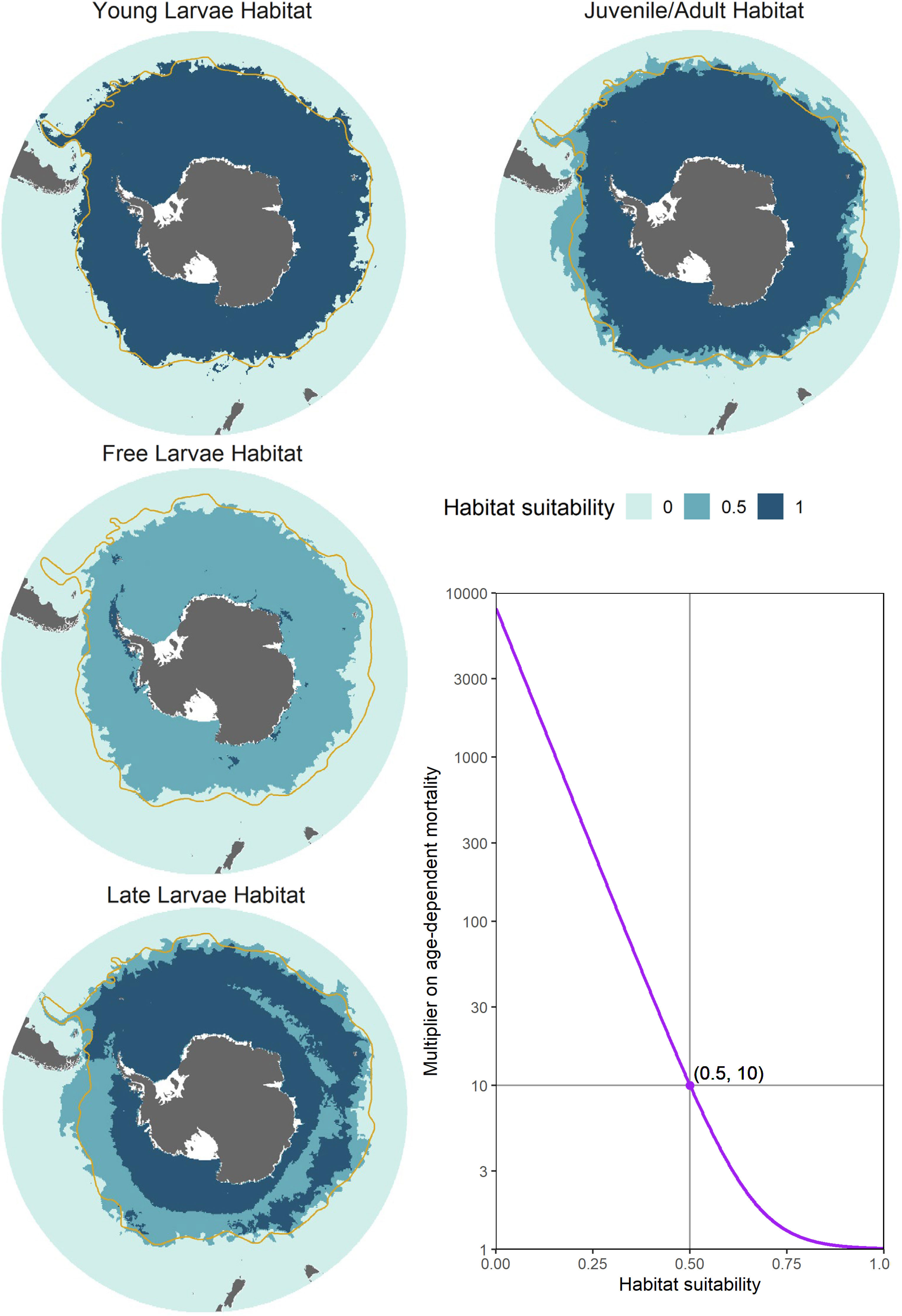
Figure 4 Illustration of computed habitat suitabilities for the five different life stages (left and top panels), along with the exponential function used to scale habitat-dependent mortality (bottom right panel). Each plotted habitat shows input for a single model timestep, representative of the period in which each life stage is in high relative abundance. In order of life stage, these habitats represent the first week of January, April, July and October. In the figure denoting the exponential mortality function (bottom right), habitat values of 1, 0.5, and 0 generate, respectively, mortality rate multipliers of 1, 10, and a value approaching 10000, which effectively enforces complete mortality. The orange line denotes the approximate climatological location of the Subantarctic Front (Orsi et al., 1995).

TABLE 2

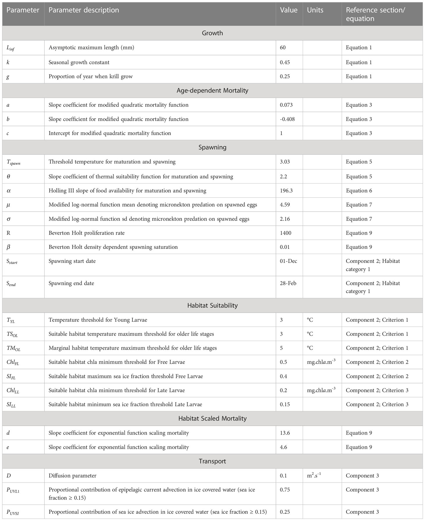
Table 2 Descriptions and initial values for parameters used in each KRILLPODYM model component.

$\begin{array}{ll}f(Adults)=\frac{R·Adults·H_s}{1.0+\beta ·Adults}& (8)\end{array}$

2.1.2.2 Habitat category 2: habitats modifying survival of life stages

Biophysical conditions are known to have a strong influence on krill survival. Furthermore, as krill transition through different developmental stages, each with unique morphological and physiological characteristics, their specific environmental requirements for survival change. This is particularly true for larval krill, which have limited capacity for dealing with reduced food availability (Ross and Quetin, 1989). To represent these specific requirements, we compute five separate habitats to modify survival of each life stage (i.e. habitats for young larvae, free larvae, late larvae, juveniles, and adults; Figure 4).

These habitats incorporate three key criteria, namely: thermal suitability (affecting survival of all life stages of krill), and sea ice conditions affecting free larvae survival, and late larvae survival. For each of these criteria we classify suitability as one of three scores: suitable (1), marginal (0.5) or unsuitable (0).

Criterion 1: Thermal suitability – Throughout their life cycle, krill remain highly stenothermic (survival restricted to a narrow temperature range), growing best in temperature < 2°C (Atkinson et al., 2006). At higher temperatures, heightened aerobic activity (Tarling, 2020) and a shortened inter-moult period (Kawaguchi et al., 2007) place stress on the capacity for individuals to maintain a positive energy balance. At temperatures > 5°C, metabolic constraints likely exceed capabilities for ingesting and assimilating sufficient food supplies to maintain energy balance (Atkinson et al., 2006; Tarling, 2020). Similarly, reduced hatching success and increased deformity rates in Young Larvae are associated with temperatures exceeding 3°C (Perry et al., 2020). We represent these requirements by using the 3°C isotherm as a threshold between suitable and unsuitable thermal conditions for Young Larvae, and in older life stages define thermal habitat as suitable up to 3°C, marginal from 3-5°C, and unsuitable in waters warmer than 5°C (see Figure 4).

In calculating thermal habitat for Young Larvae we consider average temperature across the three depth layers represented by SEAPODYM (epipelagic, upper mesopelagic and lower mesopelagic). These layers define the vertical distribution of young larvae during the descent/ascent cycle. For older life stages, which generally occur closer to the surface, we use epipelagic temperatures to calculate thermal habitat. Here, thermal suitability alone encompasses habitat conditions for young larvae, juveniles, and adults, but is combined with additional habitats for the free larvae and late larvae stages, which require specific feeding conditions to survive (detailed below).

Criterion 2: Feeding conditions affecting free larvae survival – Following the descent/ascent cycle, larval krill (calyptopes) transition into the free larvae stage and must immediately begin feeding (Ross and Quetin, 1989). However, unlike older life stages (Furcilia IV-) they lack fully developed thoracic appendages for grazing on sea ice algae (Jia et al., 2014). Survival of free larvae krill is therefore restricted to regions where there is sufficient available food in the water column (predominantly phytoplankton). Based on literature, we define suitable Free Larvae feeding habitat as the co-occurrence of chlorophyll a concentrations $\ge 0.5$ mg.chla.m^-3 (Ross and Quetin, 1989; Piñones and Fedorov, 2016; Trebilco et al., 2019) and sea ice concentrations < 40% (Thorpe et al., 2019).

Realised Free Larvae habitat (values of 1) is then computed as the combination of thermal habitat and feeding conditions. Suitable habitat coincides with the co-occurrence of suitable thermal and feedings conditions, marginal habitat occurs in association with suitable or marginal thermal conditions (< 5°C) but poor feeding conditions, and unsuitable habitat occurs where temperatures are > 5°C, irrespective of feeding conditions (Figure 4).

Criterion 3: Feeding conditions affecting late larvae survival – During winter, primary production across much of the Southern Ocean is greatly reduced. Larval krill (late larvae) do not have sufficient energy reserves to fast over extended periods (Meyer and Oettl, 2005). Where sea ice is present, late larvae (furcilia IV-) can increase food intake through grazing on sea ice communities (Frazer, 2002). Recent work has also shown that overwintering larvae can survive in ice-free waters provided there is sufficient primary production (Walsh et al., 2020; Veytia et al., 2022). In some cases, small size classes are capable of maintaining positive growth in chla concentrations as low as 0.2 mg.C.m^-3 (Tarling et al., 2006).

Consequently, we assume that suitable Late Larvae habitat (values of 1) occurs under sea ice (sea ice fraction of $\ge 15$ %; e.g. Worby, 2004), or in open waters < 3°C with chl a concentrations of $\ge 0.2$ mg.C.m^-3. Marginal habitat (values of 0.5) consists of waters of 3-5°C, or waters < 3°C and chl a concentrations < 0.2 mg.C.m^-3. As with the other life stages, waters > 5°C are considered unsuitable for survival (values of 0).

2.1.2.3 Enforcing habitat driven mortality

Habitat suitability scores, as computed above, are then used to scale age-dependent mortality such that suitable habitat has no effect on baseline (Eq. 3.) mortality rates, but forces an exponential decrease in survival as habitat suitability approaches zero. We implement this by incorporating our habitat suitability within the following exponential function (Eq. 9),

$\begin{array}{ll}f(H)=1+e^{(d·(1-H)-e)}& (9)\end{array}$

where H represents habitat suitability, while coefficients $d$ and $e$ modulate the slope of the function. In this first implementation, we have parameterised this function such that age-dependent mortality increases by an order of magnitude in marginal habitat (values of 0.5), and approaches total mortality in unsuitable habitat (values of 0; see Figure 4).

2.1.3 Component 3: enacting transport across life stages

Spatial redistribution of biomass for each age class and timestep is calculated based on the prevailing circulation of ocean currents and seasonal sea ice. To enact these spatial dynamics, implementation of this model will use methods already implemented and published in SEAPODYM. Age classes are redistributed by the underlying circulation using advection-diffusion-reaction equations, which are numerically solved across a regular grid and timestep (Lehodey et al., 2008; Senina et al., 2020), to generate spatially dynamic density fields. This approach considers both directed advection by currents (and sea ice) as well as random animal movements related to density within a given cell (diffusion). This method is well suited to describing dynamics over large spatial and temporal scales. Variables, and associated sources, used to represent these circulation patterns are detailed in ESM Table S1.

In this model, we compute two separate forms of transport, which are related to the vertical distribution and behaviour of krill at different developmental stages. The first form considers transport of young larvae (model stage 1), while the second encompasses transport of all older life stages.

Transport of young larvae (model stage 1) – Following spawning, eggs and nauplii undergo a descent/ascent cycle lasting approximately one month (Hofmann et al., 1992). During this time, they cover a range of depths spanning 0 and ~ 1000 m (Hofmann et al., 1992), and their transport is a function of currents occurring throughout this depth range. To apply this, we assume young larvae are redistributed by the average current velocities across all three depth layers (epipelagic, upper mesopelagic and lower mesopelagic; Figure 1) represented in SEAPODYM. In doing so, we compute eastward and northward current velocity fields across all three depth layers represented within SEAPODYM, with values weighted by the relative thickness of each layer. It is worth noting that while this simple metric would likely produce low advection rates, it may still over represent time spent within the upper 200m of the water column (Hofmann et al., 1992), where advection rates are highest.

Transport of free larvae, late larvae, juveniles, and adults (model stages 2 – 5) – Once krill return to surface waters as free larvae, they generally occur within the upper 200 m of the water column (e.g. Godlewska and Klusek, 1987; Bestley et al., 2018). From this point, we consider their movement to be driven by epipelagic currents in ice-free regions and by a combination of epipelagic currents and sea-ice dynamics when associated with ice (Thorpe et al., 2007; Veytia et al., 2021). To represent this, for cells within the sea ice zone (> 15% sea ice concentration) we compute a weighted mean such that epipelagic current contribute 75% and sea-ice velocities 25% to the composite advection field (equivalent to 18h in water column and 6h with ice). We note here that previous work has used a 12h split between ocean current and sea ice advection (e.g. Meyer et al., 2017; Veytia et al., 2021). However, we found here that a higher weighting (e.g. 12h/12h) of sea ice advection led to krill being advected further northwards, beyond their observed distribution (see ESM Figure S2).

2.2 KRILLPODYM simulation spin up

In this first implementation of KRILLPODYM we initialise the model using a 12-year spin up (approximately two full krill generation cycles), repeating forcings for the year 2010. The spatial domain of this implementation covers the circumpolar Southern Ocean and extends northwards from the Antarctic coast to 40° S at a horizontal grid resolution of 0.25°x 0.25°. As initial conditions we assume a uniform density (1 ind.m^-2 per age class; Figure S1) across the full spatial domain. The model advances with a weekly time step, and at each step generates spatially resolved density fields for all age classes, which are subsequently aggregated by life stage (as in Table 1).

3 Results

3.1 Spatial patterns in computed habitats

3.1.1 Habitat category 1: spawning Habitat

The spatial distribution of high quality spawning habitat was the same as that outlined in Green et al., 2021 for austral summer. Briefly, the highest quality spawning habitat in Dec-Feb, occurred along the Antarctic continent, particularly around Prydz Bay, and the region from the Ross Sea eastwards to the northern Antarctic Peninsula, extending offshore past South Georgia to the Scotia Arc (as shown in Figure 3 and also described in Green et al., 2021, Figure 2). Moderate quality spawning habitat was supported by oceanic waters further north.

3.1.2 Habitat category 2: habitats modifying survival of life stages

This initial model utilised relatively simple habitat rules for classifying suitability and modulating age-dependent survival of cohorts. Thermal constraints were the most important driver of mortality, rendering habitats north of the Subantarctic Front (~ 5°C) largely unsuitable for all krill life stages (Figure 4). Within the suitable thermal range, habitats had fairly uniform suitability for Young Larvae, Juveniles, and Adults. The strictest controls on habitat-influenced survival and distribution occurred during the Free Larvae stage, where suitable feeding conditions were primarily restricted to the Antarctic coast, as well as waters around South Georgia (as shown in Figure 4). At the Late Larvae stage, slightly more relaxed controls on survival and distribution effectively only limited survival in low productivity waters north of the Antarctic convergence spanning the Indian and Pacific Sectors of the Southern Ocean.

3.2 Model spin-up and evolution of krill spatial distribution and dynamics

3.2.1 Modelled krill distribution

During model spin-up, it took approximately 2-6 iterations for the distribution and dynamics of all life stages to stabilise, linked with the timing of adult recruitment (2 years) and maximum lifespan (6 years) (see spin up animation in ESM). Initially, uniform krill density was assumed across the entire spatial domain; however, high temperature-linked mortality rates in the north rapidly constrained the latitudinal distribution of all life stages to waters south of the Subantarctic Front (Figure 5). Spatial patterns in krill biomass developed mainly from areas of cold water and high primary production, supporting both large summer pulses of spawning activity and subsequent survival of Free Larvae. Transport by ocean currents and sea ice advection served to progressively broaden cohort distributions as they aged through later life stages. High biomasses of juveniles and younger life stages were largely contained within the maximum winter ice extent, with high densities also occurring around South Georgia. Adult krill exhibited the broadest distribution, extending well downstream of South Georgia, into the Indian Sector of the Southern Ocean (Figure 5). The model predicted the highest biomasses of krill along the Antarctic coastal band stretching eastwards from the eastern edge of the Ross Sea to South Georgia across all life stages. Approximately 65% of all post-larval krill biomass (juveniles and adults combined) occurred within the Atlantic sector stretching between CCAMLR Subareas 88.3 and 48.6 (Table 3). However, high post-larval krill abundances were also evident for other locations along the Antarctic coast; particularly the Amundsen and western Ross seas, as well as moderate biomasses across coastal East Antarctica and the Cosmonauts Sea (Figure 5).

FIGURE 5

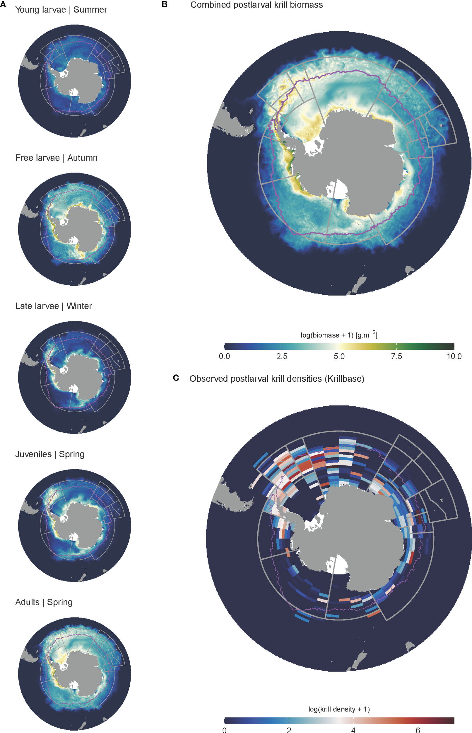
Figure 5 Modelled and observed distributions of krill. (A) denotes the biomass distributions of the different life stages in the final iteration of the model spin up. Each represents a mean biomass associated with the season in which each life stage is in highest relative abundance. (B) denotes the biomass distribution of all post-larval krill, representing the combined biomass of juveniles and adults. (C) gives observed post-larval krill densities obtained from KRILLBASE Atkinson et al. (2017). Maximum sea ice extent is given by the pink line.

TABLE 3

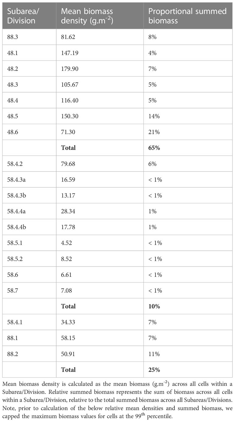
Table 3 Mean biomass density and relative summed biomass of post-larval krill for CCAMLR Subarea/Division.

3.2.2 Spatial dynamics of krill biomass

Particularly noticeable from the model spin up was the significant influence of ocean currents and sea ice advection on krill biomass redistribution. Krill biomass downstream of South Georgia was advected progressively eastward with increasing age, while there was a contrasting westward and, in some cases, northward propagation of biomass from areas of high larval production along the Antarctic coast stretching from the Weddell Sea to East Antarctica. For instance, high larval biomasses spawned in Prydz Bay were transported westwards, reaching the margin between the Cooperation and Cosmonauts Seas as Late Larvae, whereafter some were advected further west, while others were entrained in the northward sea ice advance (see spin up animation in ESM). Ultimately these larvae recruited into the juvenile population across a band stretching from the Cosmonauts Seas to the southern Kerguelen Plateau (Figure 5).

Spatial mismatches between spawned larvae and recruitment into the post larval population were not evident everywhere. Most notably, the distribution of life stages was relatively uniform in the high biomass region between the eastern edge of the Ross Sea and northern Antarctic Peninsula, with a high proportion of spawned larvae seemingly retained within these systems as they aged.

3.3 Modelled versus observed krill distributions

The modelled distribution of post-larval krill (juveniles and adults combined) showed broad similarities with observed krill distributions estimated from KRILLBASE (the most comprehensive observation database available; Atkinson et al., 2017). Both modelled and observed distributions indicated that the bulk of biomass was located within the southwest Atlantic, particularly around the Antarctic Peninsula and Scotia Sea (Figures 5, 6), and that moderate to low krill densities occurred within Indian and western Pacific sectors. Differences in modelled and observed densities were however apparent in the eastern Pacific sector, where our model predicted high krill densities in coastal Antarctic waters of the Ross, Amundsen and Bellingshausen Seas, whereas observations suggest that krill are largely absent from these areas (Figure 5).

FIGURE 6

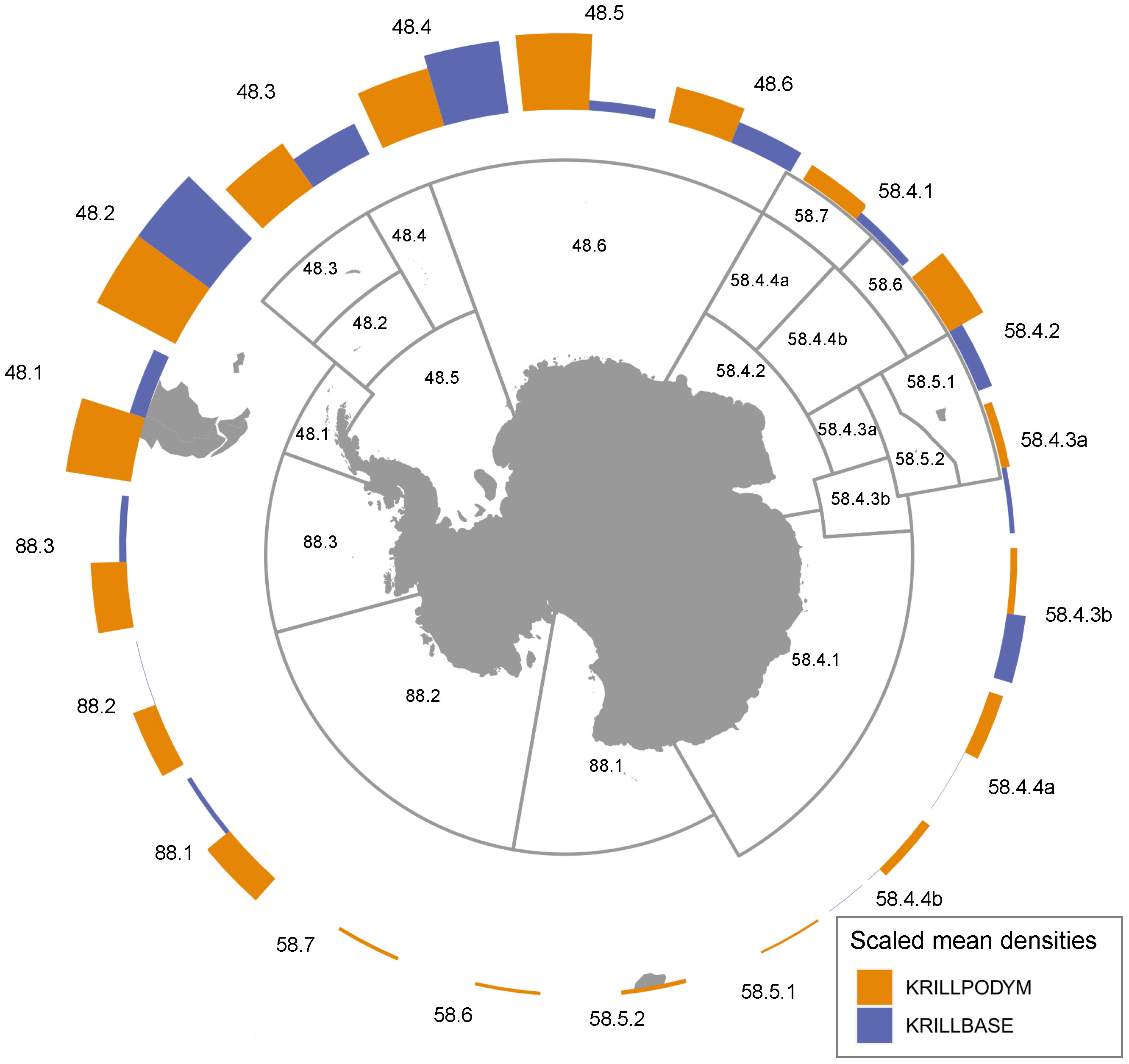
Figure 6 Modelled and observed relative (scaled 0-1) mean densities of krill, aggregated by CCAMLR Subarea/Division. Observed post-larval krill densities are derived from KRILLBASE Atkinson et al. (2017). Relative krill densities are computed by first computing mean densities at a 50km resolution, and subsequently taking the mean of all 50km cells occurring within each Subarea/Division. Relative densities are then computed by dividing each by the maximum mean density across all Subareas/Divisions. Note, prior to calculation of the below relative mean densities and summed biomass, we capped the maximum biomass values for cells at the 99^th percentile.

4 Discussion

Our key aim here was to provide a “proof-of-concept” for our novel krill model configuration, KRILLPODYM, that allows joint consideration of life history, habitat, and transport processes. Seeded with a uniform initial density, and using only a basic parameterisation based predominantly on simple thresholds, we have illustrated the model’s capacity to reproduce Antarctic krill’s circumpolar distribution and spatial dynamics. This represents a foundational step in generating highly resolved distribution and abundance estimates for a relatively data poor species (outside of the south Atlantic). The model framework also provides flexibility for future work to develop simulation experiments testing key biological processes including population processes such as growth, mortality, and reproduction, and environmental influences through exploring specific habitat requirements and advective processes.

4.1 Contrasting modelled vs observed circumpolar krill distribution

Output from this implementation indicated that the model could reasonably represent krill distribution, and regional abundances as they are currently understood. Particularly noticeable was the dominance (65%; Table 3) of modelled biomass in the south Atlantic, which aligns well with previous work that found 70% of krill biomass was concentrated between 0-90°W (Atkinson et al., 2009). Also interesting were regions that our model predicted to support high biomasses of krill, but for which observations indicate much lower densities. In the south Atlantic, such discrepancies may partly be explained by fisheries (e.g. Subarea 48.1 where much of the fishery is concentrated; see Figure 6 and Meyer et al., 2020) and consumption by predators (e.g. mesopelagics, baleen whales, seals and penguins; Saunders et al., 2019; Savoca et al., 2021; Hoffman et al., 2022; Warwick-Evans et al., 2022) remaining unaccounted for in our current model setup. Future work should consider the role of fishery catch and consumption by predators in shaping the dynamics of krill within the region. Beyond the south Atlantic, many regions of the Southern Ocean remain relatively poorly sampled for krill. As such, the discrepancy in abundance within these regions could highlight regions of relatively low sampling effort, where krill have gone largely undetected. For example, there are few KRILLBASE observations for the western Ross Sea, where our model predicts moderate to high densities of krill, which matches with independent surveys of the region (Davis et al., 2017). Further, while there is a regional paucity of directed krill sampling, it is known that the Ross Sea region has historically been an important foraging area for krill-eating whales (Branch et al., 2007). Over the course of the 1920s several thousand blue whales (Balaenoptera musculus) were taken from continental slope waters of the Ross Sea, indicating an abundant population of this species, until its extirpation in the 1930s (Branch et al., 2007; Ainley, 2010). Such large numbers of blue whales would almost certainly have required a much greater regional biomass of krill than apparent in the observed krill densities denoted in Figure 5. Indeed, the aggregations of whales along the Ross Sea continental slope suggest that our model may in fact be underestimating krill biomass here (Branch et al., 2007; Murase et al., 2013). Such findings highlight the potential value in considering indicator species distributions during model parameterisation and evaluation, particularly within regions that have received relatively little directed sampling.

In other regions, such as the Amundsen and Weddell Seas, it is unclear whether the high simulated krill biomasses here are a true reflection of the environment. Indeed, while both seas remain relatively poorly observed, the few dedicated sampling efforts within these regions have indicated that their zooplankton communities are dominated by ice krill (La et al., 2015; E. crystallorophias), rather than Antarctic krill (Wilson et al., 2015). One reason for this might be that there are competition effects between the two species, which are not accounted for within the model. Alternatively, our model habitats may not have adequately captured underlying environmental conditions modifying krill survival. Both the Amundsen and Weddell Seas are known to maintain exceptionally thick and persistent sea ice (Kurtz and Markus, 2012; Stammerjohn et al., 2015). These ice regimes could limit primary production both in the water column and within the sea ice itself, restricting feeding opportunities for krill, particularly during the Free and Late Larvae stages (Meyer et al., 2017). While the current model implementation does consider sea ice presence, it does not yet consider how sea ice characteristics, such as thickness or rugosity (Veytia et al., 2021), could modify the suitability of under ice habitat for krill survival. The role of sea ice characteristics in influencing krill survival, growth and recruitment has been highlighted as a key knowledge gap, and is one that the KRILLPODYM framework is well placed to address in future iterations.

Also notable was the broader northward distribution of modelled vs observed krill in the Atlantic and Indian sectors, particularly for the adult life stage. This highlights the role advective processes play in shaping krill’s distribution. Most obvious, was the progressive ACC-driven eastward transport of krill spawned in the southwest Atlantic as they age. However, our findings during model initialisation also indicated that sea ice advection had an important, but counter-intuitive influence on northward krill transport. Along coastal Antarctica, spawned krill appeared to be entrained in the advancing sea ice, and advected northwards, but were thereafter released into the open waters as sea ice retreated. This effectively served to push krill northward beyond ice-dominated systems, increasing its relative densities in open ocean habitats outside the maximum ice extent. Indeed, early model initialisations indicated that transport schemes of 12h/12h epipelagic currents and sea ice transport (following previous work; e.g. Meyer et al., 2017; Veytia et al., 2021) led to a much more northerly distribution of krill, while a transport regime driven entirely by epipelagic currents served to aggregate krill biomass over the Antarctic shelf, leading to much higher densities in Antarctic waters (especially the western Ross Sea; see ESM Figures S2, S3). These initial results emphasise the sensitivity of krill’s distribution to different transport mechanisms.

A notable feature of krill’s known distribution is that high biomasses are supported in the vicinity of South Georgia (Atkinson et al., 2008), but not at similar latitudes in the Indian sector, despite similar temperature regimes (see Figure 4). In this implementation, we have only considered the role of temperature in shaping suitable habitat for post-larval krill. However, previous work modelling krill growth rates has demonstrated a strong link between temperature-linked metabolism and food requirements in krill (Atkinson et al., 2006; Murphy et al., 2017; Veytia et al., 2020). For example, under temperature stress krill must feed at higher rates to maintain a positive energy balance (Atkinson et al., 2006; Hill et al., 2013). Indeed, while post-larval krill within suitable thermal habitat are able to maintain positive energy balances during periods of low food availability, at higher temperatures increased metabolic demands means that this is less feasible (Constable and Kawaguchi, 2018). Persistence of the South Georgia krill stock at its thermal limits (Tarling, 2020) is therefore likely because of the persistence of elevated primary production for much of the year (Atkinson et al., 2001). Eastwards of this, between the Scotia Arc and the Kerguelen Plateau, annual primary production within this latitudinal band is much lower (Arrigo et al., 2008). This suggests a potentially reduced capacity of these waters to maintain post-larval krill survival. Another mechanism which could be explored further is the role of heterotrophy (feeding on zooplankton such as copepods; Atkinson et al., 2002) in shaping feeding habitat quality for overwintering post-larval krill. The interplay between food availability and temperature on post-larval krill survival and subsequent distribution could be explored directly through modifying modelled juvenile and adult habitat suitability within future model iterations.

4.2 Future experiments addressing knowledge gaps in krill spatial ecology

As a first model implementation we have used published deterministic functions to represent krill life history, together with relatively simple habitat requirements and advection regimes. However, the model framework is highly flexible, allowing for parameter testing and interchangeability of the growth, mortality, and stock-recruitment functions. Likewise, because the habitats and advection fields are input as forcings, these can be recomputed offline to reflect more sophisticated relationships between krill life stages and their ocean-ice environment. This provides exciting scope for targeted experiments with the biological parameterisation, as well as testing theorised mechanisms dictating krill population processes and interactions with the biophysical environment. Future studies should use sensitivity analyses to identify how different configurations of key habitat forcings (including temperature as well as primary and secondary production) and ocean-ice advection mechanisms, influence the abundance, distribution and dynamics of krill.

Considering our model components, sensitivity analyses could focus on the following three priority areas:

1. Sensitive population parameters - Our model represents krill growth, mortality, and reproduction using deterministic functions and, wherever possible, parameter values derived from literature. While these functions and parameters are based on empirical data, most values are derived at a regional population level (e.g. Pakhomov, 1995b), and may not be fully generalisable across the full spatial domain. Sensitivity analyses considering a range of biologically feasible parameter values (and functions), would generate important understanding on how different representations of these key population processes could influence krill’s spatio-temporal population dynamics and age structure. Foremost of these should be exploring population responses to changes in the stock-recruit relationship modulating larval production.

2. Habitat suitability – Habitat suitability plays an important role in shaping krill population processes and subsequent distribution. Indeed, changes in the distribution of suitable habitat can have profound effects on overall krill abundance and distribution. This is especially true for changes in larval krill habitat suitability (e.g. Free Larvae), which have the strictest requirements. However, these suitability scores are likely also important for post-larval krill given the interacting roles of temperature and food availability on growth, as discussed above. Future model experiments could consider the sensitivity of krill spatio-temporal dynamics to different habitat scores across life stages with the aim of identifying which habitats have the greatest impact on distribution and abundance. Key experiments should explore model sensitivity to increase resolution of: 1) under ice habitat suitability, and 2) thermal – feeding habitat suitability (including the role of heterotrophy) for all krill life stages older than Young Larvae.

3. Transport processes – The role of advective processes in shaping krill distribution and metapopulation dynamics continues to be an important knowledge gap. Here we have shown that applying different relative influences of ocean currents and sea ice transport can lead to very different krill distributions across the circumpolar Southern Ocean (Figure 4 and ESM Figures 2, 3). We have assumed that krill are partly advected by sea ice in waters of > 15% cover. However, krill’s association with sea ice, and subsequent transport dynamics is certainly more complex than this. Following work on under-ice characteristics (above), future experiments should explore model sensitivity to the relative contribution of ocean currents and ice advection to krill transport.

4.3 KRILLPODYM potential applications

Here we have presented a model framework and implementation that reasonably captures the circumpolar distribution of Antarctic krill, while concurrently demonstrating the sensitivity of krill dynamics to different forcing mechanisms (e.g. transport). In so doing, we have highlighted the model’s potential for testing key assumptions on krill biology and guiding formulation of new hypotheses for improved ecosystem understanding (Cury et al., 2008; Seidl, 2017). Additionally, KRILLPODYM’s capacity to match observed spatial patterns in sampled regions suggests that it could provide a promising avenue for extending our understanding to systems sampled less frequently. Once fully parameterised, KRILLPODYM should provide a powerful operational tool for studies exploring sustainable krill fishery management, as well as broader ecological questions on ecosystem functioning. Given the flexible model framework, future KRILLPODYM iterations could also incorporate forcings computed from climate projection models (e.g. CMIP; Eyring et al., 2016), to generate projections of krill population dynamics over the upcoming decades.

4.3.1 Source-sink dynamics and krill harvest scenarios

A key challenge in sustainable management of the krill fishery is characterising metapopulation dynamics and the sources of different regional krill populations. Through its highly resolved spatial processes the model could expand capacity for identifying source-sink dynamics between different krill stocks which could subsequently be applied to harvest scenarios to investigate consequences of krill harvesting (i.e. removal of biomass from selected grid cells) on local and downstream abundance. This would be an important step towards improving understanding of how krill harvesting could impact dependent ecosystem components, including krill-eating predators (Hinke et al., 2017; Lowther et al., 2020).

4.3.2 Evaluating predator foraging habitat in a changing Southern Ocean

Our capacity to represent bottom-up trophic linkages spanning environment – predators is central to understanding Southern Ocean ecosystem responses to a changing climate. Models representing highly resolved spatial estimates of mid-trophic levels are important tools for providing synoptic forage information for higher predators (e.g. Green et al., 2020; Romagosa et al., 2021; Green et al., 2023). As an operational product, KRILLPODYM would open opportunities for investigating the foraging habitat of krill-dependent marine predators (e.g. baleen whales, crabeater seals, Adelie and chinstrap penguins) based on direct spatio-temporal estimates of their prey. Using an implementation forced by climate projection models, established links between krill and predator foraging could then be projected into upcoming decades, generating valuable insights into potential future ecosystem structure. Furthermore, by reconciling model representations of krill with knowledge derived from both direct (active sampling, e.g. KRILLBASE; Atkinson et al., 2017) and indirect observations (e.g. through indicator species such as baleen whales; Alvarez and Orgeira, 2022), we can arrive at a more integrated representation of these remote and inaccessible ecosystems (Santora et al., 2013; Santora et al., 2021).

Data availability statement

The datasets presented in this study can be found in online repositories. Output from this first model initialisation can be found on the Institute for Marine and Antarctic Studies (IMAS) Data Portal (https://doi.org/10.25959/895K-K978).

Author contributions

All authors contributed towards model conceptualisation. DG coordinated the project, model initialisation, and wrote the initial manuscript, while OT adapted SEAPODYM model programming and structure for KRILLPODYM. All authors contributed biological and technical expertise, reviewed and commented on the manuscript. All authors contributed to the article and approved the submitted version.

Funding

This research was supported by the Australian Research Council Special Research Initiative, Australian Centre for Excellence in Antarctic Science (Project Number SR200100008). DG received funding through a Tasmania Graduate Research Scholarship. SB was supported by the Australian Research Council under DECRA award DE180100828. Further funding was provided through the European H2020 International Cooperation project Mesopelagic Southern Ocean Prey and Predators No 692173.

Acknowledgments

The authors thank Bettina Fach and Stephanie Brodie for useful comments on a previous version of this manuscript.

Conflict of interest

The authors declare that the research was conducted in the absence of any commercial or financial relationships that could be construed as a potential conflict of interest.

Publisher’s note

All claims expressed in this article are solely those of the authors and do not necessarily represent those of their affiliated organizations, or those of the publisher, the editors and the reviewers. Any product that may be evaluated in this article, or claim that may be made by its manufacturer, is not guaranteed or endorsed by the publisher.

Supplementary material

The Supplementary Material for this article can be found online at: https://www.frontiersin.org/articles/10.3389/fmars.2023.1218003/full#supplementary-material

References

Abecassis M., Lehodey P., Senina I., Polovina J. J., Calmettes B., Williams P. (2011). Application of the SEAPODYM model to swordfish in the pacific ocean (Pacific Islands Fisheries Science Center: US Department of Commerce, National Oceanic and Atmospheric Administration, National Marine Fisheries Service).

Google Scholar

Ainley D. G. (2010). A history of the exploitation of the ross sea, antarctica. Polar Rec. 46, 233–243. doi: 10.1017/S003224740999009X

CrossRef Full Text | Google Scholar

Alvarez F., Orgeira J. (2022). Krill finder: spatial distribution of sympatric fin (Balaenoptera physalus) and humpback (Megaptera novaeangliae) whales in the southern ocean. Polar Biol. 45, 1427–1440. doi: 10.1007/s00300-022-03080-x

CrossRef Full Text | Google Scholar

Arrigo K. R., Van Dijken G. L., Bushinsky S. (2008). Primary production in the southern ocean, 1997–2006 J. Geophys. Res 113, C08004. doi: 10.1029/2007jc004551

CrossRef Full Text | Google Scholar

Atkinson A., Hill S. L., Pakhomov E. A., Siegel V., Anadon R., Chiba S., et al. (2017). KRILLBASE: a circumpolar database of Antarctic krill and salp numerical densities 1926–2016. Earth System Sci. Data 9, 193–210. doi: 10.5194/essd-9-193-2017

CrossRef Full Text | Google Scholar

Atkinson A., Hill S. L., Pakhomov E. A., Siegel V., Reiss C. S., Loeb V. J., et al. (2019). Krill (Euphausia superba) distribution contracts southward during rapid regional warming. Nat. Climate Change 9, 142–147. doi: 10.1038/s41558-018-0370-z

CrossRef Full Text | Google Scholar

Atkinson A., Meyer B., Stuϋbing D., Hagen W., Schmidt K., Bathmann U. V. (2002). Feeding and energy budgets of Antarctic krill Euphausia superba at the onset of winter-II. juveniles and adults. Limnology Oceanography 47, 953–966. doi: 10.4319/lo.2002.47.4.0953

CrossRef Full Text | Google Scholar

Atkinson A., Shreeve R. S., Hirst A. G., Rothery P., Tarling G. A., Pond D. W., et al. (2006). Natural growth rates in Antarctic krill (Euphausia superba): II. predictive models based on food, temperature, body length, sex, and maturity stage. Limnology Oceanography 51, 973–987. doi: 10.4319/lo.2006.51.2.0973

CrossRef Full Text | Google Scholar

Atkinson A., Siegel V., Pakhomov E., Jessopp M., Loeb V. (2009). A re-appraisal of the total biomass and annual production of antarctic krill. Deep Sea Res. Part I: Oceanographic Res. Papers 56, 727–740. doi: 10.1016/j.dsr.2008.12.007

CrossRef Full Text | Google Scholar

Atkinson A., Siegel V., Pakhomov E. A., Rothery P., Loeb V., Ross R. M., et al. (2008). Oceanic circumpolar habitats of Antarctic krill. Mar. Ecol. Prog. Ser. 362, 1–23. doi: 10.3354/meps07498

CrossRef Full Text | Google Scholar

Atkinson A., Whitehouse M., Priddle J., Cripps G., Ward P., Brandon M. (2001). South georgia, antarctica: a productive, cold water, pelagic ecosystem. Mar. Ecol. Prog. Ser. 216, 279–308. doi: 10.3354/meps216279

CrossRef Full Text | Google Scholar

Bestley S., Raymond B., Gales N. J., Harcourt R. G., Hindell M. A., Jonsen I. D., et al. (2018). Predicting krill swarm characteristics important for marine predators foraging off East Antarctica. Ecography 41, 996–1012. doi: 10.1111/ecog.03080

CrossRef Full Text | Google Scholar

Branch T. A., Stafford K., Palacios D., Allison C., Bannister J., Burton C., et al. (2007). Past and present distribution, densities and movements of blue whales balaenoptera musculus in the southern hemisphere and northern indian ocean. Mammal Rev. 37, 116–175. doi: 10.1111/j.1365-2907.2007.00106.x

CrossRef Full Text | Google Scholar

Candy S. G. (2021). Long-term trend in mean density of Antarctic krill (Euphausia superba) uncertain. Annu. Res. Rev. Biol. 36, 27–43. doi: 10.9734/arrb/2021

CrossRef Full Text | Google Scholar

Candy S. G., Kawaguchi S. (2006). Modelling growth of Antarctic krill. II. novel approach to describing the growth trajectory. Mar. Ecol. Prog. Ser. 306, 17–30. doi: 10.3354/meps306017

CrossRef Full Text | Google Scholar

Carr M. H., Robinson S. P., Wahle C., Davis G., Kroll S., Murray S., et al. (2017). The central importance of ecological spatial connectivity to effective coastal marine protected areas and to meeting the challenges of climate change in the marine environment. Aquat. Conservation: Mar. Freshw. Ecosyst. 27, 6–29. doi: 10.1002/aqc.2800

CrossRef Full Text | Google Scholar

Conroy J. A., Reiss C. S., Gleiber M. R., Steinberg D. K. (2020). Linking Antarctic krill larval supply and recruitment along the Antarctic peninsula. Integr. Comp. Biol. 60, 1386. doi: 10.1093/icb/icaa111

PubMed Abstract | CrossRef Full Text | Google Scholar

Constable A. J., Kawaguchi S. (2018). Modelling growth and reproduction of Antarctic krill, Euphausia superba, based on temperature, food and resource allocation amongst life history functions. ICES J. Mar. Sci. 75, 738–750. doi: 10.1093/icesjms/fsx190

CrossRef Full Text | Google Scholar

Constable A., Nicol S. (2002). Defining smaller-scale management units to further develop the ecosystem approach in managing large-scale pelagic krill fisheries in antarctica. Ccamlr Sci. 9, 117–131.

Google Scholar

Cox M. J., Candy S., de la Mare W. K., Nicol S., Kawaguchi S., Gales N. (2018). No evidence for a decline in the density of Antarctic krill Euphausia superba Dana 1850, in the southwest Atlantic sector between 1976 and 2016. J. Crustacean Biol. 38, 656–661. doi: 10.1093/jcbiol/ruy072

CrossRef Full Text | Google Scholar

Cury P. M., Shin Y.-J., Planque B., Durant J. M., Fromentin J.-M., Kramer-Schadt S., et al. (2008). Ecosystem oceanography for global change in fisheries. Trends Ecol. Evol. 23, 338–346. doi: 10.1016/j.tree.2008.02.005

PubMed Abstract | CrossRef Full Text | Google Scholar

Daly K. L. (2004). Overwintering growth and development of larval Euphausia superba: an interannual comparison under varying environmental conditions west of the Antarctic peninsula. Deep Sea Res. Part II: Topical Stud. Oceanography 51, 2139–2168. doi: 10.1016/j.dsr2.2004.07.010

CrossRef Full Text | Google Scholar

Davis L. B., Hofmann E. E., Klinck J. M., Piñones A., Dinniman M. S. (2017). Distributions of krill and antarctic silverfish and correlations with environmental variables in the western ross sea, antarctica. Mar. Ecol. Prog. Ser. 584, 45–65. doi: 10.3354/meps12347

CrossRef Full Text | Google Scholar

Dragon A.-C., Senina I., Hintzen N., Lehodey P. (2018). Modelling south pacific jack mackerel spatial population dynamics and fisheries. Fisheries Oceanography 27, 97–113. doi: 10.1111/fog.12234

CrossRef Full Text | Google Scholar

Eyring V., Bony S., Meehl G. A., Senior C. A., Stevens B., Stouffer R. J., et al. (2016). Overview of the coupled model intercomparison project phase 6 (cmip6) experimental design and organization. Geoscientific Model. Dev. 9, 1937–1958. doi: 10.5194/gmd-9-1937-2016

CrossRef Full Text | Google Scholar

Fach B. A., Klinck J. M. (2006). Transport of Antarctic krill (Euphausia superba) across the Scotia sea. part I: circulation and particle tracking simulations. Deep Sea Res. Part I: Oceanographic Res. Papers 53, 987–1010. doi: 10.1016/j.dsr.2006.03.006

CrossRef Full Text | Google Scholar

Frazer T. K. (2002). Abundance, sizes and developmental stages of larval krill, Euphausia superba, during winter in ice-covered seas west of the Antarctic peninsula. J. Plankton Res. 24, 1067–1077. doi: 10.1093/plankt/24.10.1067

CrossRef Full Text | Google Scholar

Godlewska M., Klusek Z. (1987). Vertical distribution and diurnal migrations of krill ? Euphausia superba Dana ? from hydroacoustical observations, SIBEX, December 1983/January 1984. Polar Biol. 8, 17–22. doi: 10.1007/bf00297159

CrossRef Full Text | Google Scholar

Green D. B., Bestley S., Corney S. P., Trebilco R., Lehodey P., Hindell M. A. (2021). Modeling Antarctic krill circumpolar spawning habitat quality to identify regions with potential to support high larval production. Geophysical Res. Lett. 48, e2020GL091206. doi: 10.1029/2020GL091206

CrossRef Full Text | Google Scholar

Green D. B., Bestley S., Corney S. P., Trebilco R., Makhado A. B., Lehodey P., et al. (2023). Modelled prey fields predict marine predator foraging success. Ecol. Indic. 147, 109943. doi: 10.1016/j.ecolind.2023.109943

CrossRef Full Text | Google Scholar

Green D. B., Bestley S., Trebilco R., Corney S. P., Lehodey P., McMahon C. R., et al. (2020). Modelled mid-trophic pelagic prey fields improve understanding of marine predator foraging behaviour. Ecography 43, 1014–1026. doi: 10.1111/ecog.04939

CrossRef Full Text | Google Scholar

Hagen W., Auel H. (2001). Seasonal adaptations and the role of lipids in oceanic zooplankton. presented at the 94th annual meeting of the deutsche zoologische gesellschaft in osnabrück, June 4–8, 2001. Zoology 104, 313–326. doi: 10.1078/0944-2006-00037

PubMed Abstract | CrossRef Full Text | Google Scholar

Hernandez O., Lehodey P., Senina I., Echevin V., Ayón P., Bertrand A., et al. (2014). Understanding mechanisms that control fish spawning and larval recruitment: parameter optimization of an eulerian model (SEAPODYM-SP) with Peruvian anchovy and sardine eggs and larvae data. Prog. Oceanogr. 123, 105–122. doi: 10.1016/j.pocean.2014.03.001

CrossRef Full Text | Google Scholar

Hill S. L., Phillips T., Atkinson A. (2013). Potential climate change effects on the habitat of Antarctic krill in the weddell quadrant of the southern ocean. PloS One 8, e72246. doi: 10.1371/journal.pone.0072246

PubMed Abstract | CrossRef Full Text | Google Scholar

Hinke J. T., Cossio A. M., Goebel M. E., Reiss C. S., Trivelpiece W. Z., Watters G. M. (2017). Identifying risk: concurrent overlap of the Antarctic krill fishery with krill-dependent predators in the Scotia Sea. PloS One 12, e0170132. doi: 10.1371/journal.pone.0170132

PubMed Abstract | CrossRef Full Text | Google Scholar

Hoffman J. I., Chen R. S., Vendrami D. L., Paijmans A. J., Dasmahapatra K. K., Forcada J. (2022). Demographic reconstruction of antarctic fur seals supports the krill surplus hypothesis. Genes 13, 541. doi: 10.3390/genes13030541

PubMed Abstract | CrossRef Full Text | Google Scholar

Hofmann E. E., Capella J. E., Ross R. M., Quetin L. B. (1992). Models of the early life history of Euphausia superba–part i. time and temperature dependence during the descent-ascent cycle. Deep Sea Res. Part I. Oceanographic Res. Papers 39, 1177–1200. doi: 10.1016/0198-0149(92)90063-Y

CrossRef Full Text | Google Scholar

Hofmann E. E., Hüsrevoğlu Y. S. (2003). A circumpolar modeling study of habitat control of Antarctic krill (Euphausia superba) reproductive success. Deep Sea Res. Part II: Topical Stud. Oceanography 50, 3121–3142. doi: 10.1016/j.dsr2.2003.07.012

CrossRef Full Text | Google Scholar

Hosie G. W., Ikeda T., Stolp M. (1988). Distribution, abundance and population structure of the Antarctic krill (Euphausia superba Dana) in the prydz bay region, Antarctica. Polar Biol. 8, 213–224. doi: 10.1007/bf00443453

CrossRef Full Text | Google Scholar

Ikeda T. (1984). Development of the larvae of the Antarctic krill (Euphausia superba Dana) observed in the laboratory. J. Exp. Mar. Biol. Ecol. 75, 107–117. doi: 10.1016/0022-0981(84)90175-8

CrossRef Full Text | Google Scholar

Jia Z., Virtue P., Swadling K. M., Kawaguchi S. (2014). A photographic documentation of the development of Antarctic krill (Euphausia superba) from egg to early juvenile. Polar Biol. 37, 165–179. doi: 10.1007/s00300-013-1420-7

CrossRef Full Text | Google Scholar

Jones B. T., Solow A., Ji R. (2016). Resource allocation for lagrangian tracking. J. Atmospheric Oceanic Technol. 33, 1225–1235. doi: 10.1175/jtech-d-15-0115.1

CrossRef Full Text | Google Scholar

Ju S.-J., Harvey H. R. (2004). Lipids as markers of nutritional condition and diet in the Antarctic krill Euphausia superba and Euphausia crystallorophias during austral winter. Deep Sea Res. Part II: Topical Stud. Oceanography 51, 2199–2214. doi: 10.1016/j.dsr2.2004.08.004

CrossRef Full Text | Google Scholar

Kawaguchi S. (2016). “Reproduction and larval development in Antarctic krill (Euphausia superba),” in Biology and ecology of Antarctic krill. Ed. Siegel V. (Basel, Switzerland: Springer), 225–246. doi: 10.1007/978-3-319-29279-3_6

CrossRef Full Text | Google Scholar

Kawaguchi S., Satake M. (1994). Relationship between recruitment of the Antarctic krill and the degree of ice cover near the south Shetland islands. Fisheries Sci. 60, 123–124. doi: 10.2331/fishsci.60.123

CrossRef Full Text | Google Scholar

Kawaguchi S., Yoshida T., Finley L., Cramp P., Nicol S. (2007). The krill maturity cycle: a conceptual model of the seasonal cycle in Antarctic krill. Polar Biol. 30, 689–698. doi: 10.1007/s00300-006-0226-2

CrossRef Full Text | Google Scholar

Krüger L., Huerta M. F., Santa Cruz F., Cárdenas C. A. (2021). Antarctic Krill fishery effects over penguin populations under adverse climate conditions: implications for the management of fishing practices. Ambio 50, 560–571. doi: 10.1007/s13280-020-01386-w

PubMed Abstract | CrossRef Full Text | Google Scholar

Kurtz N. T., Markus T. (2012). Satellite observations of antarctic sea ice thickness and volume. J. Geophysical Research: Oceans 117. doi: 10.1029/2012JC008141

CrossRef Full Text | Google Scholar

La H. S., Lee H., Fielding S., Kang D., Ha H. K., Atkinson A., et al. (2015). High density of ice krill (euphausia crystallorophias) in the amundsen sea coastal polynya, antarctica. Deep Sea Res. Part I: Oceanographic Res. Papers 95, 75–84. doi: 10.1016/j.dsr.2014.09.002

CrossRef Full Text | Google Scholar

Lancelot C., Mathot S., Veth C., de Baar H. (1993). Factors controlling phytoplankton ice-edge blooms in the marginal ice-zone of the northwestern Weddell Sea during sea ice retreat 1988: field observations and mathematical modelling. Polar Biol. 13, 377−387.

Google Scholar

Lehodey P. (2004). A spatial ecosystem and populations dynamics model (SEAPODYM) for tuna and associated oceanic top-predator species: part I – lower and intermediate trophic components (Noumea, New Caledonia: Oceanic Fisheries Programme, Secretariat of the Pacific Community).

Google Scholar

Lehodey P., Conchon A., Senina I., Domokos R., Calmettes B., Jouanno J., et al. (2015). Optimization of a micronekton model with acoustic data. ICES J. Mar. Sci. 72, 1399–1412. doi: 10.1093/icesjms/fsu233

CrossRef Full Text | Google Scholar

Lehodey P., Murtugudde R., Senina I. (2010). Bridging the gap from ocean models to population dynamics of large marine predators: a model of mid-trophic functional groups. Prog. Oceanogr. 84, 69–84. doi: 10.1016/j.pocean.2009.09.008

CrossRef Full Text | Google Scholar

Lehodey P., Senina I., Murtugudde R. (2008). A spatial ecosystem and populations dynamics model (SEAPODYM)–modeling of tuna and tuna-like populations. Prog. Oceanogr. 78, 304–318. doi: 10.1016/j.pocean.2008.06.004

CrossRef Full Text | Google Scholar

Levin S. A. (1992). The problem of pattern and scale in ecology: the Robert h. MacArthur award lecture. Ecology 73, 1943–1967. doi: 10.2307/1941447

CrossRef Full Text | Google Scholar

Loeb V. J., Hofmann E. E., Klinck J. M., Holm-Hansen O., White W. B. (2009). ENSO and variability of the Antarctic peninsula pelagic marine ecosystem. Antarctic Sci. 21, 135–148. doi: 10.1017/s0954102008001636

CrossRef Full Text | Google Scholar

Lowther A. D., Staniland I., Lydersen C., Kovacs K. M. (2020). Male Antarctic Fur seals: neglected food competitors of bioindicator species in the context of an increasing Antarctic krill fishery. Sci. Rep. 10, 1–12. doi: 10.1038/s41598-020-75148-9

PubMed Abstract | CrossRef Full Text | Google Scholar

Marrari M., Daly K. L., Hu C. (2008). Spatial and temporal variability of SeaWiFS chlorophyll a distributions west of the Antarctic peninsula: implications for krill production. Deep Sea Res. Part II: Topical Stud. Oceanography 55, 377–392. doi: 10.1016/j.dsr2.2007.11.011

CrossRef Full Text | Google Scholar

Maury O. (2010). An overview of APECOSM, a spatialized mass balanced “Apex predators ECOSystem model” to study physiologically structured tuna population dynamics in their ecosystem. Prog. Oceanogr. 84, 113–117. doi: 10.1016/j.pocean.2009.09.013

CrossRef Full Text | Google Scholar

McCormack S. A., Melbourne-Thomas J., Trebilco R., Blanchard J. L., Constable A. (2020). Alternative energy pathways in southern ocean food webs: insights from a balanced model of prydz bay, antarctica. Deep Sea Res. Part II: Topical Stud. Oceanography 174, 104613. doi: 10.1016/j.dsr2.2019.07.001

CrossRef Full Text | Google Scholar

Melbourne-Thomas J., Corney S. P., Trebilco R., Meiners K. M., Stevens R. P., Kawaguchi S., et al. (2016). Under ice habitats for Antarctic krill larvae: could less mean more under climate warming? Geophys. Res. Lett. 43, 10322–10327. doi: 10.1002/2016gl070846

CrossRef Full Text | Google Scholar

Meyer B., Atkinson A., Bernard K. S., Brierley A. S., Driscoll R., Hill S. L., et al. (2020). Successful ecosystem-based management of Antarctic krill should address uncertainties in krill recruitment, behaviour and ecological adaptation. Commun. Earth Environ. 1, 1–12. doi: 10.1038/s43247-020-00026-1

CrossRef Full Text | Google Scholar

Meyer B., Atkinson A., Stöbing D., Oettl B., Hagen W., Bathmann U. V. (2002). Feeding and energy budgets of Ant arctic krill Euphausia superba at the onset of winter. I.Furcilia III larvae. Limnol. Oceanogr.47, 943−952.

Google Scholar

Meyer B., Freier U., Grimm V., Groeneveld J., Hunt B. P. V., Kerwath S., et al. (2017). The winter pack-ice zone provides a sheltered but food-poor habitat for larval Antarctic krill. Nat. Ecol. Evol. 1, 1853–1861. doi: 10.1038/s41559-017-0368-3

PubMed Abstract | CrossRef Full Text | Google Scholar

Meyer B., Oettl B. (2005). Effects of short-term starvation on composition and metabolism of larval Antarctic krill euphausia superba. Mar. Ecol. Prog. Ser. 292, 263–270. doi: 10.3354/meps292263

CrossRef Full Text | Google Scholar

Mori M., Corney S. P., Melbourne-Thomas J., Klocker A., Kawaguchi S., Constable A., et al. (2019). Modelling dispersal of juvenile krill released from the Antarctic ice edge: ecosystem implications of ocean movement. J. Mar. Syst. 189, 50–61. doi: 10.1016/j.jmarsys.2018.09.005

CrossRef Full Text | Google Scholar

Murase H., Kitakado T., Hakamada T., Matsuoka K., Nishiwaki S., Naganobu M. (2013). Spatial distribution of antarctic minke whales (b alaenoptera bonaerensis) in relation to spatial distributions of krill in the ross sea, antarctica. Fisheries Oceanography 22, 154–173. doi: 10.1111/fog.12011

CrossRef Full Text | Google Scholar

Murphy E. J., Thorpe S. E., Tarling G. A., Watkins J. L., Fielding S., Underwood P. (2017). Restricted regions of enhanced growth of Antarctic krill in the circumpolar southern ocean. Sci. Rep. 7, 6963. doi: 10.1038/s41598-017-07205-9

PubMed Abstract | CrossRef Full Text | Google Scholar

Murphy E. J., Watkins J. L., Trathan P. N., Reid K., Meredith M. P., Thorpe S. E., et al. (2007). Spatial and temporal operation of the Scotia Sea ecosystem: a review of large-scale links in a krill centred food web. Philos. Trans. R. Soc. B: Biol. Sci. 362, 113–148. doi: 10.1098/rstb.2006.1957

CrossRef Full Text | Google Scholar

Nicol S., Foster J., Kawaguchi S. (2012). The fishery for Antarctic krill - recent developments. Fish Fisheries 13, 30–40. doi: 10.1111/j.1467-2979.2011.00406.x

CrossRef Full Text | Google Scholar

Orsi A. H., Whitworth T., Nowlin W. D. (1995). On the meridional extent and fronts of the Antarctic circumpolar current. Deep Sea Res. Part I: Oceanographic Res. Papers 42, 641–673. doi: 10.1016/0967-0637(95)00021-w

CrossRef Full Text | Google Scholar

Pakhomov E. A. (1995a). Demographic studies of Antarctic krill Euphausia superba in the cooperation and cosmonaut seas (Indian sector of the southern ocean). Mar. Ecol. Prog. Ser. 119, 45–61. doi: 10.3354/meps119045

CrossRef Full Text | Google Scholar

Pakhomov E. A. (1995b). Natural age-dependent mortality rates of Antarctic krill Euphausia superba Dana in the Indian sector of the southern ocean. Polar Biol. 15, 69–71. doi: 10.1007/BF00236127

CrossRef Full Text | Google Scholar

Perry F. A., Kawaguchi S., Atkinson A., Sailley S. F., Tarling G. A., Mayor D. J., et al. (2020). Temperature–induced hatch failure and nauplii malformation in Antarctic krill. Front. Mar. Sci. 7. doi: 10.3389/fmars.2020.00501

CrossRef Full Text | Google Scholar

Piñones A., Fedorov A. V. (2016). Projected changes of Antarctic krill habitat by the end of the 21st century. Geophys. Res. Lett. 43, 8580–8589. doi: 10.1002/2016GL069656

CrossRef Full Text | Google Scholar

Rassweiler A., Ojea E., Costello C. (2020). Strategically designed marine reserve networks are robust to climate change driven shifts in population connectivity. Environ. Res. Lett. 15, 34030. doi: 10.1088/1748-9326/ab6a25

CrossRef Full Text | Google Scholar

Romagosa M., Pérez-Jorge S., Cascão I., Mouriño H., Lehodey P., Pereira A., et al. (2021). Food talk: 40-Hz fin whale calls are associated with prey biomass. Proc. R. Soc. B: Biol. Sci. 288, 20211156. doi: 10.1098/rspb.2021.1156

CrossRef Full Text | Google Scholar

Rosenberg A. A., Beddington J. R., Basson M. (1986). Growth and longevity of krill during the first decade of pelagic whaling. Nature 324, 152–154. doi: 10.1038/324152a0

CrossRef Full Text | Google Scholar

Ross R. M., Quetin L. B. (1989). Energetic cost to develop to the first feeding stage of Euphausia superba Dana and the effect of delays in food availability. J. Exp. Mar. Biol. Ecol. 133, 103–127. doi: 10.1016/0022-0981(89)90161-5

CrossRef Full Text | Google Scholar

Ryabov A. B., De Roos A. M., Meyer B., Kawaguchi S., Blasius B. (2017). Competition-induced starvation drives large-scale population cycles in Antarctic krill. Nat. Ecol. Evol. 1, 1–8. doi: 10.1038/s41559-017-0177

PubMed Abstract | CrossRef Full Text | Google Scholar

Santora J. A., Rogers T. L., Cimino M. A., Sakuma K. M., Hanson K. D., Dick E., et al. (2021). Diverse integrated ecosystem approach overcomes pandemic-related fisheries monitoring challenges. Nat. Commun. 12, 6492. doi: 10.1038/s41467-021-26484-5

PubMed Abstract | CrossRef Full Text | Google Scholar

Santora J. A., Sydeman W. J., Messié M., Chai F., Chao Y., Thompson S. A., et al. (2013). Triple check: observations verify structural realism of an ocean ecosystem model. Geophysical Res. Lett. 40, 1367–1372. doi: 10.1002/grl.50312

CrossRef Full Text | Google Scholar

Saunders R. A., Hill S. L., Tarling G. A., Murphy E. J. (2019). Myctophid fish (family myctophidae) are central consumers in the food web of the Scotia Sea (Southern ocean). Front. Mar. Sci. 6. doi: 10.3389/fmars.2019.00530

CrossRef Full Text | Google Scholar

Savoca M. S., Czapanskiy M. F., Kahane-Rapport S. R., Gough W. T., Fahlbusch J. A., Bierlich K., et al. (2021). Baleen whale prey consumption based on high-resolution foraging measurements. Nature 599, 85–90. doi: 10.1038/s41586-021-03991-5

PubMed Abstract | CrossRef Full Text | Google Scholar

Schmidt K., Atkinson A., Venables H. J., Pond D. W. (2012). Early spawning of Antarctic krill in the Scotia Sea is fuelled by “superfluous” feeding on non-ice associated phytoplankton blooms. Deep Sea Res. Part II: Topical Stud. Oceanography 59, 159–172. doi: 10.1016/j.dsr2.2011.05.002

CrossRef Full Text | Google Scholar

Seidl R. (2017). To model or not to model, that is no longer the question for ecologists. Ecosystems 20, 222–228. doi: 10.1007/s10021-016-0068-x

PubMed Abstract | CrossRef Full Text | Google Scholar

Senina I. N., Lehodey P., Sibert J., Hampton J. (2020). Integrating tagging and fisheries data into a spatial population dynamics model to improve its predictive skills. Can. J. Fisheries Aquat. Sci. 77 (3), 576–593. doi: 10.1139/cjfas-2018-0470

CrossRef Full Text | Google Scholar

Senina I. N., Sibert J., Lehodey P. (2008). Parameter estimation for basin-scale ecosystem-linked population models of large pelagic predators: application to skipjack tuna. Prog. Oceanogr. 78, 319–335. doi: 10.1016/j.pocean.2008.06.003

CrossRef Full Text | Google Scholar

Siegel V. (2012). Krill stocks in high latitudes of the Antarctic lazarev Sea: seasonal and interannual variation in distribution, abundance and demography. Polar Biol. 35, 1151–1177. doi: 10.1007/s00300-012-1162-y

CrossRef Full Text | Google Scholar

Siegel V., Loeb V. (1994). Length and age at maturity of Antarctic krill. Antarctic Sci. 6, 479–482. doi: 10.1017/s0954102094000726

CrossRef Full Text | Google Scholar

Siegel V., Watkins J. L. (2016). “Distribution biomass and demography of Antarctic krill euphausia superba,” in Biology and ecology of Antarctic krill. Ed. Siegel V. (Basel, Switzerland: Springer), 21–100.

Google Scholar

Spiridonov V. (1995). Spatial and temporal variability in reproductive timing of Antarctic krill (Euphausia superba Dana). Polar Biol. 15, 161–174. doi: 10.1007/bf00239056

CrossRef Full Text | Google Scholar

Stammerjohn S., Maksym T., Massom R., Lowry K., Arrigo K., Yuan X., et al. (2015). Seasonal sea ice changes in the amundsen sea, antarctica, over the period of 1979–2014 seasonal sea ice changes in the amundsen sea. Elementa: Sci. Anthropocene 3. doi: 10.12952/journal.elementa.000055

CrossRef Full Text | Google Scholar

Tarling G. A. (2020). Routine metabolism of Antarctic krill (Euphausia superba) in south Georgia waters: absence of metabolic compensation at its range edge. Mar. Biol. 167, 1–15. doi: 10.1007/s00227-020-03714-w

CrossRef Full Text | Google Scholar

Tarling G. A., Shreeve R. S., Hirst A. G., Atkinson A., Pond D. W., Murphy E. J., et al. (2006). Natural growth rates in Antarctic krill (Euphausia superba): i. improving methodology and predicting intermolt period. Limnol. Oceanogr. 51, 959–972. doi: 10.4319/lo.2006.51.2.0959

CrossRef Full Text | Google Scholar

Thorpe S. E., Murphy E. J., Watkins J. L. (2007). Circumpolar connections between Antarctic krill (Euphausia superba Dana) populations: investigating the roles of ocean and sea ice transport. Deep Sea Res. Part I: Oceanographic Res. Papers 54, 792–810. doi: 10.1016/j.dsr.2007.01.008

CrossRef Full Text | Google Scholar

Thorpe S. E., Tarling G. A., Murphy E. J. (2019). Circumpolar patterns in Antarctic krill larval recruitment: an environmentally driven model. Mar. Ecol. Prog. Ser. 613, 77–96. doi: 10.3354/meps12887

CrossRef Full Text | Google Scholar

Trebilco R., Melbourne-Thomas J., Sumner M., Wotherspoon S., Constable A. (2019). Assessing status and trends of open ocean habitats: a regionally resolved approach and southern ocean application. Ecol. Indic. 107, 105616. doi: 10.1016/j.ecolind.2019.105616

CrossRef Full Text | Google Scholar

Treml E. A., Halpin P. N., Urban D. L., Pratson L. F. (2008). Modeling population connectivity by ocean currents, a graph-theoretic approach for marine conservation. Landscape Ecol. 23, 19–36. doi: 10.1007/s10980-007-9138-y

CrossRef Full Text | Google Scholar

Veytia D., Bestley S., Kawaguchi S., Meiners K. M., Murphy E. J., Fraser A. D., et al. (2021). Overwinter sea-ice characteristics important for Antarctic krill recruitment in the southwest Atlantic. Ecol. Indic. 129, 107934. doi: 10.1016/j.ecolind.2021.107934

CrossRef Full Text | Google Scholar

Veytia D., Bestley S., Meiners K., Kawaguchi S., Murphy E., Kusahara K., et al. (2022). Quality of sea-ice habitat traversed by Antarctic krill larvae influences recruitment success. Res. Square. doi: 10.21203/rs.3.rs-1255733/v1

CrossRef Full Text | Google Scholar

Veytia D., Corney S., Meiners K. M., Kawaguchi S., Murphy E. J., Bestley S. (2020). Circumpolar projections of Antarctic krill growth potential. Nat. Climate Change 10, 568–575. doi: 10.1038/s41558-020-0758-4

CrossRef Full Text | Google Scholar

Walsh J., Reiss C., Watters G. (2020). Flexibility in Antarctic krill Euphausia superba decouples diet and recruitment from overwinter sea-ice conditions in the northern Antarctic peninsula. Mar. Ecol. Prog. Ser. 642, 1–19. doi: 10.3354/meps13325

CrossRef Full Text | Google Scholar

Warwick-Evans V., Kelly N., Dalla Rosa L., Friedlaender A., Hinke J., Kim J., et al. (2022). Using seabird and whale distribution models to estimate spatial consumption of krill to inform fishery management. Ecosphere 13, e4083. doi: 10.1002/ecs2.4083

CrossRef Full Text | Google Scholar

Wiedenmann J., Cresswell K. A., Mangel M. (2009). Connecting recruitment of Antarctic krill and sea ice. Limnol. Oceanogr. 54, 799–811. doi: 10.4319/lo.2009.54.3.0799

CrossRef Full Text | Google Scholar

Wilson S. E., Swalethorp R., Kjellerup S., Wolverton M. A., Ducklow H. W., Yager P. L. (2015). Meso-and macro-zooplankton community structure of the amundsen sea polynya, antarctica (summer 2010–2011) zooplankton community structure of the amundsen sea polynya, antarctica. Elementa: Sci. Anthropocene 3. doi: 10.12952/journal.elementa.000033

CrossRef Full Text | Google Scholar

Worby A. (2004). Studies of the Antarctic sea ice edge and ice extent from satellite and ship observations. Remote Sens. Environ. 92, 98–111. doi: 10.1016/j.rse.2004.05.007

CrossRef Full Text | Google Scholar