Reconstruction of subsurface ocean state variables using Convolutional Neural Networks with combined satellite and in situ data

1 Introduction

Accurate monitoring of regional and global ocean state is crucial for a full understanding of Earth system dynamics and for the detailed assessment of critical impacts of anthropogenic pressures on climate and marine ecosystems (Stewart, 2009; Bindoff et al., 2019). Central to this is the distributions of essential ocean variables (EOVs), such as temperature and salinity, as well as their interactions over a wide range of spatial and temporal scales both in horizontal and vertical dimensions (Moltmann et al., 2019).

To improve our observing capability and to enable process-based modelling efforts, ocean observing systems based on both in situ and remote sensing platforms have been continuously improving, focusing on the collection of EOVs data at the highest possible resolution (Stewart, 2009). Various remote sensing platforms and sensors are used today for ocean monitoring, and the number of satellites dedicated to Earth Observation has increased substantially over the last 40 years (Amani et al., 2022). Satellite data have rather uniform spatial and temporal coverage, but they are limited to the surface of the ocean and can be inherently noisy and error-prone, requiring different levels of postprocessing (Yueh et al., 2001; Castro et al., 2008). Similarly, a growing number of oceanographic cruises and automated systems (mooring, buoys, etc.) have provided in situ hydrographic measurements for decades. The collection of high-quality in situ observations has increased considerably since the introduction of the Argo program in 1999 (Roemmich et al., 2001; Wong et al., 2020) which has been able to deliver accurate temperature and salinity profiles down to a depth of 2000 m. Still, all in situ measurements, including Argo, are inherently sparse both in time and space when compared to satellite measurements. Hence it is of fundamental importance to develop methods capable of leveraging on the advantages of both observing systems to optimize the effort required in ocean data collection.

Different methods have been proposed for estimating subsurface ocean variables, such as temperature and salinity, including process-based numerical models and statistical data assimilation techniques. Some of these methods are based on a combination of ocean circulation model analyses, dynamics data, hydrographic data, and remotely-sensed data (Wunsch and Gaposchkin, 1980; Kao, 1987), while other methods are strictly data-driven and use advanced statistical models of surface and subsurface observations. Early studies (Cheney, 1982; Khedouri et al., 1983) demonstrated the value of statistical approaches in combining satellite and in situ data obtaining a high correlation between measurements of the ocean surface topography and the subsurface thermal structure. Single Empirical Orthogonal Function (EOF) reconstructions also have been found useful to couple surface values with subsurface properties using historical data (Carnes et al., 1990; Carnes et al., 1994; Buongiorno Nardelli and Santoleri, 2005). This latter framework was further developed using multivariate features (mEOF-r) achieving better results for reconstructed anomalies of temperature, salinity, and steric height (Nardelli and Santoleri, 2005; Buongiorno Nardelli et al., 2006; Nardelli et al., 2017). Various methods for subsurface variable reconstruction were reviewed by Fox et al. (2002); Guinehut et al. (2012); Jeong et al. (2019), where single and multi-coupled linear regression models were used to estimate relationships between sea surface fields, e.g., temperature and altimetry data, and profiles of ocean temperature.

Recently, deep learning approaches have been used to estimate the subsurface thermal structure for large ocean regions, demonstrating that they are effective in representing nonlinear relations between surface and subsurface variables (Ali et al., 2004; Su et al., 2020). In particular, simple feed-forward Neural Networks (NNs) have been used to reconstruct temperature profiles using sea surface variables such as temperature (SST), height (SSH), wind (SSW), net surface heat flux, net incoming shortwave and outgoing long wave radiation (Ali et al., 2004). Reconstructions from mEOF-r have been compared with those derived from NN architectures, including Long-Short-Term-Memory (LSTM) algorithms, trained on North Atlantic in situ vertical data from Argo profiles and using satellite surface measurements (temperature, salinity, and absolute dynamic topography) (Buongiorno Nardelli, 2020). Starting from quite different approaches, namely training on pre-gridded 3D fields, various LSTM and Convolutional Neural Networks (CNN) architectures have been proposed to infer the vertical ocean structure from surface data alone (Han et al., 2019; Su et al., 2021a; Su et al., 2021b).

Deep learning methods have consistently shown superior performance compared to other statistical approaches in reconstructing subsurface EOVs based on surface observations. Numerous studies have examined and demonstrated the capabilities of neural network-based frameworks in reconstructing EOVs across various environmental ocean conditions and dynamics. These studies have been conducted at regional scales such as in the Atlantic and Pacific Ocean regions (Wu et al., 2012; Zhang et al., 2020; Meng and Yan, 2022), as well as at the global scale (Lu et al., 2019; Su et al., 2020). However, most of these analyses have primarily relied on spatially gridded in situ data sets, which provide spatially consistent representations of the ocean state but restrict the reconstruction resolution and limit the use of additional information in areas with high observational density. Using direct vertical measurements on the other hand provide precise and localized information but leads to a data set with varying observation densities across different regions.

Here we build upon previous findings and propose a CNN framework for the direct reconstruction of salinity and temperature profiles, using satellite-based surface measurements across the entire Atlantic Ocean in the period 2005-2020. The present study extends previous results on the North Atlantic (Buongiorno Nardelli, 2020) by including the South Atlantic hence including regions with a relatively lower density of in situ profiles. The new CNN architecture presented here is used to cover an extensive geographical region including temperate, tropical and equatorial regimes in the Atlantic Ocean. The analysis and systematic evaluation of different inputs has been expanded considerably compared to previous studies and a sensitivity analysis of the model is included to assess performances in the reconstructions against the appropriateness and quality of the input data.

In summary, the contributions of this paper include:

● A comparison of different deep learning models for reconstructing salinity and temperature, using CNN as a central deep learning architecture.

● A sensitivity analysis of various combinations of physical variables to assess performances in reconstruction (ablation study, feature importance and random input perturbations).

● An assessment of the impact of the training set size and geographical distribution on the reconstructed variables.

In Section 2, the data are introduced followed by a description of the CNN model and several baseline models for comparison. In Section 3, we present the results, compare them to several other models and show that our model can effectively reconstruct ocean state variables in the entire Atlantic Ocean. Section 4 contains a discussion of our results and in Section 5 we highlight the key findings. The Appendix, Section 6, contains Supplementary Material.

2 Materials and methods

2.1 Surface and in situ measurements

Salinity and temperature profiles are reconstructed using a CNN model trained on remotely-sensed surface data and in situ observations, including geospatial information, i.e., location and time of the sample acquisition. Satellite measurements and in situ temperature and salinity profiles in the Atlantic Ocean over the period 2005-2020 were obtained through the Copernicus Marine Environment Monitoring Service (CMEMS¹). Information about the specific products is contained in Table 1.

TABLE 1

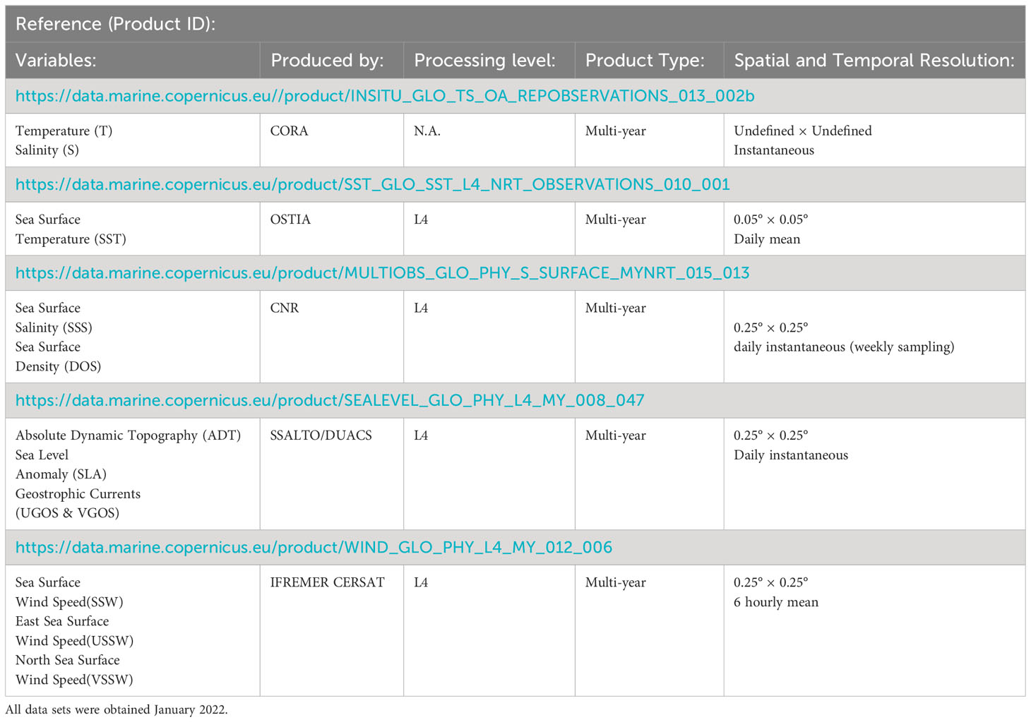
Table 1 Data set properties, origin, processing level, type, spatial and temporal resolution.

The vertical profiles included quality-controlled conductivity, temperature, and depth (CTD) produced by the Coriolis In Situ Analysis System (ISAS) (Szekely et al., 2019). These values were interpolated onto a regularly spaced vertical grid using 10 m intervals down to a depth of 1500m. Similarly, steric heights (SH), densities (D), and thermal expansion coefficients (TC) are computed on the regular grid taking 1500m as reference level. Profiles that do not extend to a depth of 1500m or with data gaps ranging more than two depth steps were discarded in the analyses, while single missing data points were estimated by linear interpolation. Accordingly, the profiles in the data set have 151 values for the depth range 0 - 1500 m with a vertical resolution of 10 m. About 50% of the available profiles in the Atlantic were removed since they did not meet these criteria.

Surface observations were acquired from several satellite platforms and obtained from four different data sets. We used and examined combinations of multi-year reprocessed L4 surface measurements of Sea Surface Temperature (SST), Salinity (SSS), Density (DOS), Absolute Dynamic Topography (ADT), Sea Level Anomaly (SLA), and geostrophic currents (UGOS & VGOS) as well as wind speeds (SSW, USSW, VSSW). The variables are on a gap-free, regular grid, but the temporal and spatial resolution of these vary (see Table 1). The UK-Metoffice OSTIA product and CNR product provide error estimates for SST and SSS, denoted here as SST_errorand SSS_error, respectively. The main source of error is from the sampling capability of the constellation of the various satellites used to create the data sets and includes factors such as data coverage, variations in biases from multiple sensors, and the statistical interpolation technique employed. Generally, they are computed using a combination of uncertainty estimates from satellite instruments and the standard deviations of the differences between measurements obtained from Argo floats and satellite observations [see details in McLaren et al. (2016); Buongiorno Nardelli et al. (2022)].

2.2 Climatological data

Climatological average fields of salinity and temperature were obtained from World Ocean Atlas 18 (WOA-18) (Locarnini et al., 2019; Zweng et al., 2019). These are objectively computed monthly profile averages on a 0.25° × 0.25° grid and using observation from the period 1981-2010, with depth up to 1500 m using 57 vertical levels. As with the in situ profiles, these data have been interpolated onto a regularly spaced vertical grid with 10 m intervals. In this work, Climatological averages have been linearly interpolated both temporally and spatially to match the day and locations of the in situ measurements, denoted interpolated climatological average (iCLIM).

Subtraction of iCLIM from measured profiles preserves only the nonseasonal, anomalous signals, allowing for the extraction and isolation of patterns, trends and variation that may be obscured by long-term averages. Climatological average profiles were subtracted from each variable to produce anomaly values of subsurface temperature (TA), salinity (SA), steric height (SHA), density (DA), and thermal expansion coefficient (TCA). Moreover, following the same procedure surface anomaly fields of each variable were produced: sea surface temperature (SSTA), salinity (SSSA), density (DOSA), and absolute dynamic topography (ADTA).

Much of the variability of global wind patterns are governed by seasonal changes and geographic location. In this work, we produce a one-year baseline data set for wind speed comprised of weekly averages over the period of 1993-2020. These baselines of weekly values were distributed with a spatial resolution of 0.25° × 0.25°. The averages were temporally and spatially smoothed using a Gaussian filter to remove high-frequency noise and isolate the underlying signal (Bourassa et al., 2005). Specifically, the Gaussian filter was applied with a standard deviation (std) of 4 in time and [2,2] in space. The values of std were determined through a series of tests and by inspecting the patterns of the weekly averages in various regions. Equivalently, to the construction of other anomaly values, the baseline values were subtracted from surface wind speed measurements to produce sea surface wind speed anomalies (SSWA).

2.3 Study area and processing of the input data

2.3.1 Study region

Data acquired from the Atlantic Ocean were used for model training and overall assessments of the models. However, to assess reconstruction on a regional level, smaller spatial regions were analyzed. These regions were selected to include highly dynamic and stable regions as well as regions of high and low observation densities. Regions were regarded as dynamic if they exhibited high anomalies with respect to the iCLIM (Figure 1B). The presence of strong mesoscale dynamics may in particular drive deviations from the climatological averages. The average std of the temperature anomaly distributions are relatively small across the entire Atlantic with an overall average std of 0.38°C, but reach values of 1.2°C in smaller local regions. It should be noted, that the deviations displayed in the figure are the average stds over full profiles, i.e., the figure does not indicate the depth at which high anomalies occur, which may vary with depth depending on the geographical location. However, the purpose of this study is to generate reliable reconstructions of full profiles, and therefore, the selection of study regions was based on std averages.

FIGURE 1

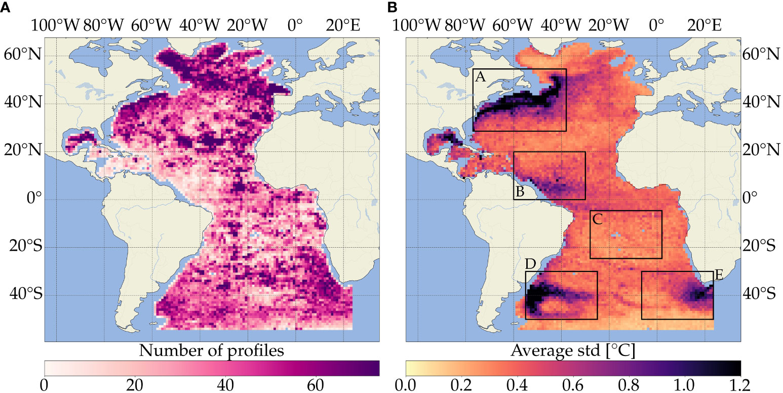
Figure 1 (A) Spatial distribution of the data points obtained in the period 2005-2020, and (B) Standard deviations (stds) of temperature anomaly profiles averaged over a 1°x 1° grid and over the full profiles for the same period (for a figure showing salinity, see in Appendix 6.1, Figure S1). Regions of dark purple colors indicate a large number of measurements deviating from the Climatology, whereas the light yellow colors indicate high consistency between WOA-18 and observed profiles. The regions (A–E) represent specific study regions.

Five areas have been selected (Figure 1B: regions A-E) to compare the reconstructions in contrasting ocean regions. The regions A, B, D, E display moderate to high stds of the anomalies. The origin of these anomalies is driven by different dynamics. Much of the dynamics in Region A are caused by variations in the Gulf

Stream, while outflow from the Amazon River has a notable effect on Region B. Region C illustrates a region that on average corresponds well with the climatological mean.

2.3.2 Data preprocessing

The total number of profiles in the period 2005-2020 within the Atlantic Ocean is slightly above 270,000. The spatial density of the profiles shows a relatively uniform distribution across the Atlantic Ocean, where the median number of observations per pixel on a 1°x 1° grid is 40, and 64% of pixels have between 20-50 observations. Certain areas appear as under sampled with 10% of pixels having less than 10 observations, and conversely, some regions include more than 70 observations per pixel cf. Figure 1A. There are several factors that may contribute to these under sampled regions, most notably the oceanic circulation as the distribution of Argo floats is strongly influenced by the surface ocean currents. Other contributing factors include the depth of the area, as profiles shallower than 1500m have been excluded, as well as the deployment distribution of Argo floats, particularly during the early stages of the program.

Surface satellite data were co-located to in situ measurements using the geographical location (latitude and longitude) of the profiles and the Julian day, and applying bilinear interpolation on the surface values. For the vast majority of data points, the surface measurements of the two platforms were consistent. The differences between satellite and in situ observations were approximately Gaussian distributed with mean −0.007°C and standard deviation (std) 0.48°C for temperature measurements, and a mean −0.017g/kg and std 0.22g/kg for salinity. Although these distributions were narrow, the ranges of the two variables are substantially different. The surface measurements of temperature were ranging from −1.7°C to 32.0°C, whereas the salinity measurements range from 30g/kg to 37.8g/kg with most measurements being above 33.5g/kg. Thus, the differences between the two types of salinity measurements were larger relative to their range than those of the temperature. These differences can be attributed to several factors, including the coarser spatial and temporal resolution of the satellite salinity data set, which may result in missed short-term and/or small-scale fluctuations detected by in situ measurements but not captured by satellites. Furthermore, notable discrepancies in salinity were observed near river outlets and estuaries, particularly associated with the Río de la Plata Estuary, as well as the Amazon, Mississippi, and Congo River outlets (See Appendix 6.2, Figure S2). Although, SSS estimates based on satellite microwave radiometer measurements in cold waters, i.e., at high latitudes, are subject to higher uncertainty (Boutin et al., 2021), no notable changes were observed in the spatial distribution of the discrepancies in these regions except for a slight increase in the Davis Strait. This may be ascribed to the calibration process carried out by CNR to generate the data set, by employing a multi-dimensional optimal interpolation algorithm using SSS data from multiple satellite sources, as well as in situ salinity measurements and satellite SST information. Additionally, it is worth noting that platform discrepancies for both salinity and particularly temperature were more pronounced in dynamic regions, something which can be attributed primarily to inconsistencies in the sampling time between observations.

Wind speed strongly influences the vertical mixing and stratification of the water column, and the response is lagged and accumulated. Therefore, the wind conditions at the point of an in situ recording may not be particularly informative. For that reason, we introduce a new variable, SSW_sumwhich represents the sum of wind speeds over the preceding 3 days. The choice of this value was based on the depth of the water column and was selected as a compromise to account for both strongly and weakly stratified regions, which can impact the mixing caused by wind.

Spatial and temporal information are used as input for the models. Latitudes (lat) and longitudes (lon) of the observations are used as inputs for the models, as well as temporal information provided as day of the year (DOY). In order to enable a neural network to learn the cyclic nature of a year, the DOY is projected onto a circle with center at (1,1) as $da{y}_1=\cos (\frac{2\pi }{365}\text{DOY})+1,\text{\hspace{0.17em}}da{y}_2=\cos (\frac{2\pi }{365}\text{DOY})+1$. Accordingly, available physical variables for model input are comprised of SST, SSS, ADT, SSW, SSWS, SSW_sum, and corresponding anomalies. The available outputs are full profiles of temperature, salinity, steric height (SH), density (D), thermal coefficient (TC), and corresponding anomalies. Each of the physical quantities is min-max normalized between [0,1] to prepare the data for a deep learning framework. To ensure model evaluations of high quality, 20% of the total size of the data set is allocated as a test set. From the remaining 80%, an additional 20% is reserved for a validation set and 80% for a training set. These are both used in the training process of the network.

2.4 Model architecture

The salinity and temperature depth profiles were reconstructed using the CNN model schematically represented in Figure 2 with hyperparameters shown in Table 2. The hyperparameters refer both to the choices of the structure of the network and other parameter values that govern parts of the learning process of a network, and they have been chosen after optimization over multiple tests. To mitigate the potential issue of the learning process becoming trapped in a local minimum, we incorporate cosine annealing into the Adam optimizer during training (Loshchilov and Hutter, 2017; Sørensen et al., 2022). This technique involves changing the learning rate at each epoch according to a cosine function with a period of E_iand a range of [η_min, η_max]. The maximum value for each cycle is decayed by η_decay. The model uses an input vector of N elements, comprising surface measurements and geospatial metadata. It produces vertical profiles of M variables, such as temperature (T), salinity (S), steric height (SH), density (D), thermal expansion coefficient (TC) and/or their respective anomalies (TA, SA, SHA, DA, and TCA). These profiles consist of 151 depth estimates with a regular spacing of 10m (total 1500m depth reconstructions). However, the present model structure enable to customize the input size N and output size M to accommodate different numbers of input and output variables.

FIGURE 2

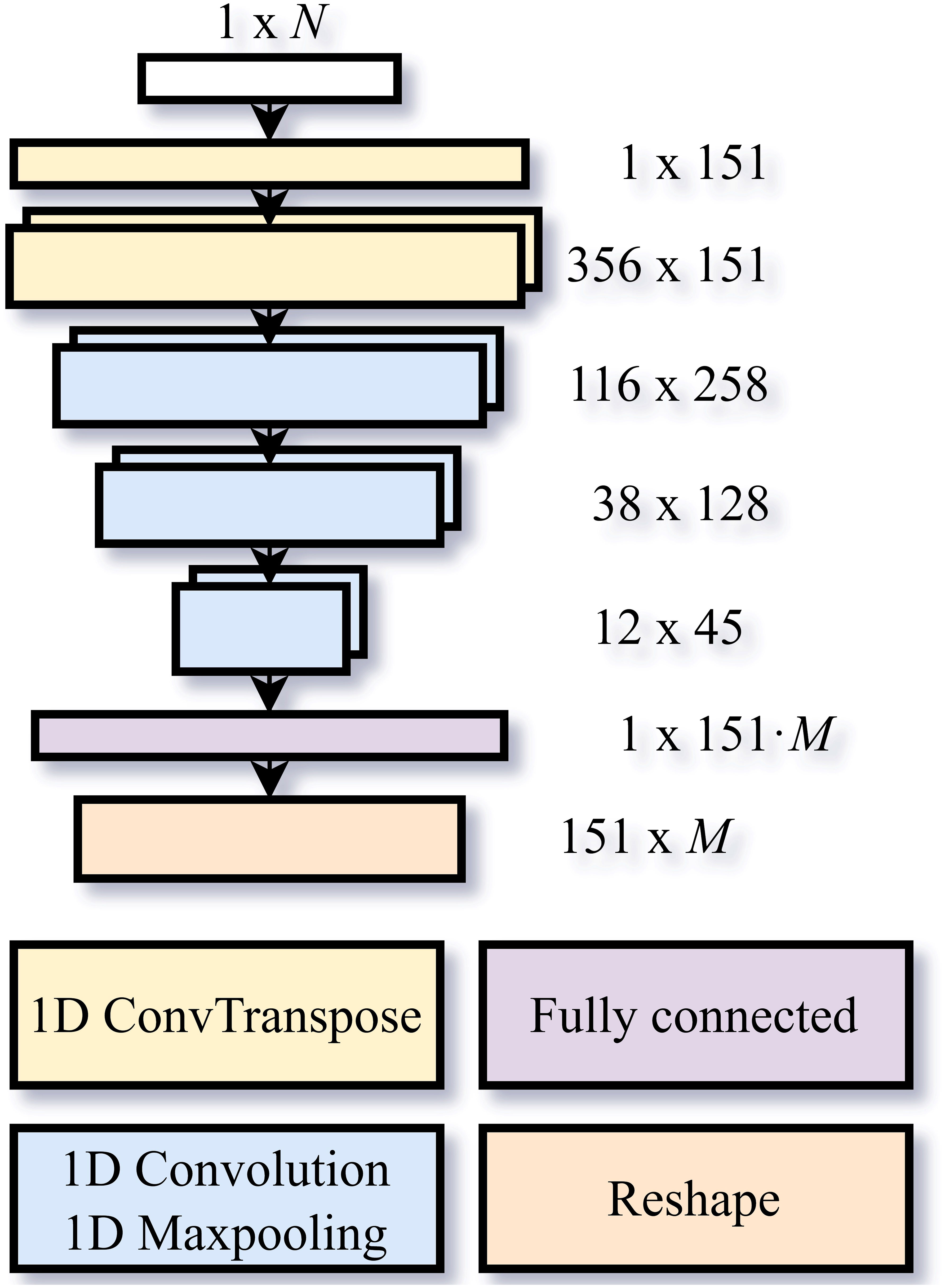
Figure 2 Diagram of the convolution neural network architecture (CNN) with N surface inputs shown on the top. The network processes information through a series of operations, each denoted by a different color, with the size of the output for each layer displayed to the right. The convolutional layers are designed with a kernel size of 3 and stride 1, and the max pooling layers are configured with a pool size of 3 and stride size of 3. The final output is estimates of M vertical profiles.

TABLE 2

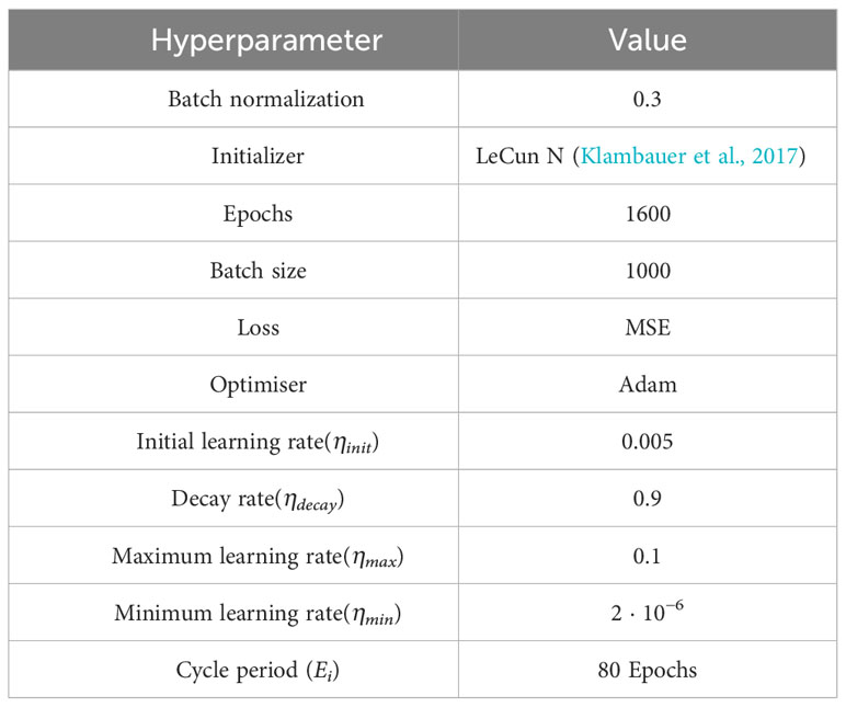
Table 2 Hyperparameters of the CNN model.

We first used one-dimensional transpose convolution layers, which act as reverse operations of a convolutional layer, to establish weights for upsampling. This process increases the size of an input matrix, while simultaneously finding weights such that important features are highlighted. Subsequently, 1D convolutional layers are used to find patterns in the upsampled input needed to infer the output, and to identify increasingly more complex patterns in the hidden layers of the network. The 1D convolutional layers are used instead of standard 2D convolutional layers to address the objective of reconstructing different 1D profiles (Kiranyaz et al., 2021). The design of the network has been decided based on extensive manual search, while other hyperparameters have been selected through a grid search.

2.5 Analyses of the results

In order to evaluate the performance of our proposed CNN model (called OCNN, see Figure 2), we compared the results of this framework with four other approaches: interpolated climatological averages (iCLIM), a long short-term memory network (LSTM), a bidirectional LSTM (BLSTM), a baseline CNN (bCNN). In stable regions, the iCLIM is a good approximation of the subsurface ocean structure. Therefore, we compared profile anomalies, generated with respect to Climatology, to the difference between model predictions and in situ observations. In addition, we implemented the state-of-the-art LSTM structure proposed in (Buongiorno Nardelli, 2020) and an advanced version [called bidirectional LSTM, i.e., BLSTM (Graves and Schmidhuber, 2005)] for further comparisons. Finally, a simple baseline CNN architecture (bCNN), is used to compare the results to demonstrate the importance of a careful design of CNN architecture for the problem at hand. Note that in addition to a simpler architecture, the hyperparameters of the bCNN have not been optimized, differently from the OCNN.

The four approaches for comparison and the OCNN are summarized as:

● Interpolated climatological averages (iCLIM): Climatological averages from WOA-18 were used as a reference.

● LSTM(35): The Long-Short-Term-Memory (LSTM) model² from (Buongiorno Nardelli, 2020), our initial benchmark for the reconstruction of ocean hydrographic structure.

● BLSTM(35): The Bidirectional-LSTM is a more advanced version of the LSTM model. This network consist of two LSTM layers in series with 35 memory cells in each layer. The architecture is identical the LSTM(35) but uses bidirectional LSTM layers.

● bCNN: A baseline CNN model with a simple architecture and without a hyperparameter optimization. It contains one fewer transpose convolutions and convolution/max-pooling block than the OCNN architecture.

● OCNN: The final CNN model, shown in Figure 2, which has been constructed by carrying hyperparameter tuning based on a grid-search.

To facilitate comparison, all neural network-based models were initially trained with the same variables as in (Buongiorno Nardelli, 2020). Here, the inputs are anomalies of sea surface temperature (SSTA), sea surface salinity (SSSA), absolute dynamic topography (ADTA) as well as latitudes, longitudes, and day of the year. The outputs of the networks are vertical anomaly profiles of temperature (TA), salinity (SA), and steric height (SHA). In this study, we used unaltered ADT values, which include both effects of steric changes (temperature and salinity variations) and eustatic variations, e.g., as those due to barotropic adjustments in response to atmospheric pressure field changes or large scale dynamical balances (e.g. in the presence of intense barotropic flows). The impact of explicitly including these different signals is unclear within the framework of neural network models, and while there are potential benefits to incorporating them in a model, their estimate can also be affected by the limited in situ data available to define an accurate steric adjustment procedure. Other studies have isolated the steric component within the ADT values (Buongiorno Nardelli, 2020), and further work may be conducted to systematically evaluate potential impacts of the decomposition of the ADT values.

The models were trained on an Nvidia A100 60 GB GPU, with an automatic termination scheme after 100 epochs with no improvement in the validation loss. All models were optimized using the Adam optimiser (Kingma and Ba, 2014) with the same parameters as in Table 2.

Variations in the importance of the inputs may indicate or highlight physical relations between the sea surface and subsurface properties and conditions, although the relations do not represent causality. One approach to obtain estimates of the relative importance of inputs uses the concept of Shapley values. In game theory, Shapley values are used to assess the contribution of each agent to the outcome of a cooperative game (Winter, 2002). Using the algorithm SHAP (SHapley Additive exPlanations)(Lundberg and Lee, 2017), we estimate the marginal contribution of each individual input feature to the final prediction of a model. Shapley values are computed for all depths to assess the change in the importance of the inputs for the model predictions at various depths.

Additionally, we implement a method for evaluating the importance based on the sensitivity, of the model to noise in the relevant input variables. Here, sensitivity is defined as the relative change in model output resulting from a relative change in input variables. Instead of finding the marginal contributions of the inputs, we here assess the direct impact of variations in the inputs on the results. By adding small random perturbations to each input of the network, the corresponding impact on the overall reconstruction performance may be approximated. Features will have relatively high importance if small changes of an input value lead to large increases in the errors of the reconstructions, and conversely. By analyzing these effects, it is possible to estimate the impacts of measurement noise on the accuracy of the reconstructions.

3 Results

3.1 Accuracy of the reconstructions

To compare the performances of the different reconstruction models, we computed the root mean squared error (RMSE) between the test set and the respective reconstruction (Table 3). Specifically, for all analyzed reconstruction methods, RMSE values are computed at each of the 151 depth levels using the entire test set, thus generating vertical RMSE profiles for every method across the whole Atlantic Ocean. The mean values represent the domain scale averages of these vertical RMSE profiles, while the maximum (Max) values are the largest RMSE values among these 151 depth levels of each method. Consistent with previous studies, the reconstructions obtained using neural network-based approaches displayed notably lower RMSE values compared to iCLIM, with OCNN showing the lowest RMSE among all analyzed methods. However, RMSE values are not constant over the water column but vary with depth (Figure 3) with generally higher values at the surface, while lower and close to zero RMSEs in the deeper layers (> 500 m). The iCLIM had the poorest performance in reconstruction at all depths, and indeed neural network models outperformed iCLIM over the entire water column for both temperature and salinity values. Specifically, RMSE values ranged from 0.17°C to 1.12°C for temperature and from 0.3 g/kg to 0.033 g/kg for salinity for all neural network methods while maximum RMSE for iCLIM is 1.4°C in temperature and 0.32 g/kg in salinity. At all depths, the OCNN outperformed all the other models in the reconstruction of both variables. The errors obtained with the OCNN are comparable to other neural network models over most of the water column. However, both CNN approaches (bCNN, OCNN) showed greater reconstruction accuracy than the LSTM models in the upper layer of the ocean. The OCNN exhibited average reconstruction errors that were 19% and 17% lower than the LSTM for temperature and salinity, respectively, in the upper 200m of the water column. Moreover, when compared to the iCLIM in this region, the OCNN showed significant improvements, with average reconstruction errors that were 39% and 30% lower for temperature and salinity, respectively. For the full water column, the average reconstruction errors of the OCNN when compared to the iCLIM were 41% and 26% lower for temperature and salinity, respectively.

TABLE 3

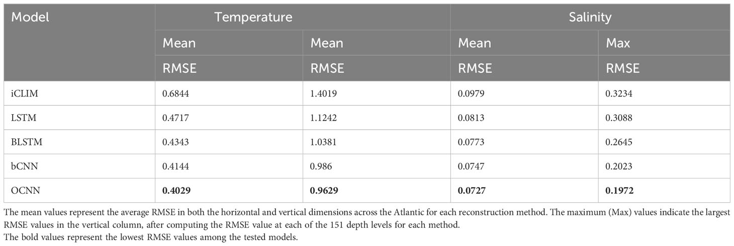
Table 3 Test score for all models for temperature and salinity measured in °C and [g/kg], respectively.

FIGURE 3

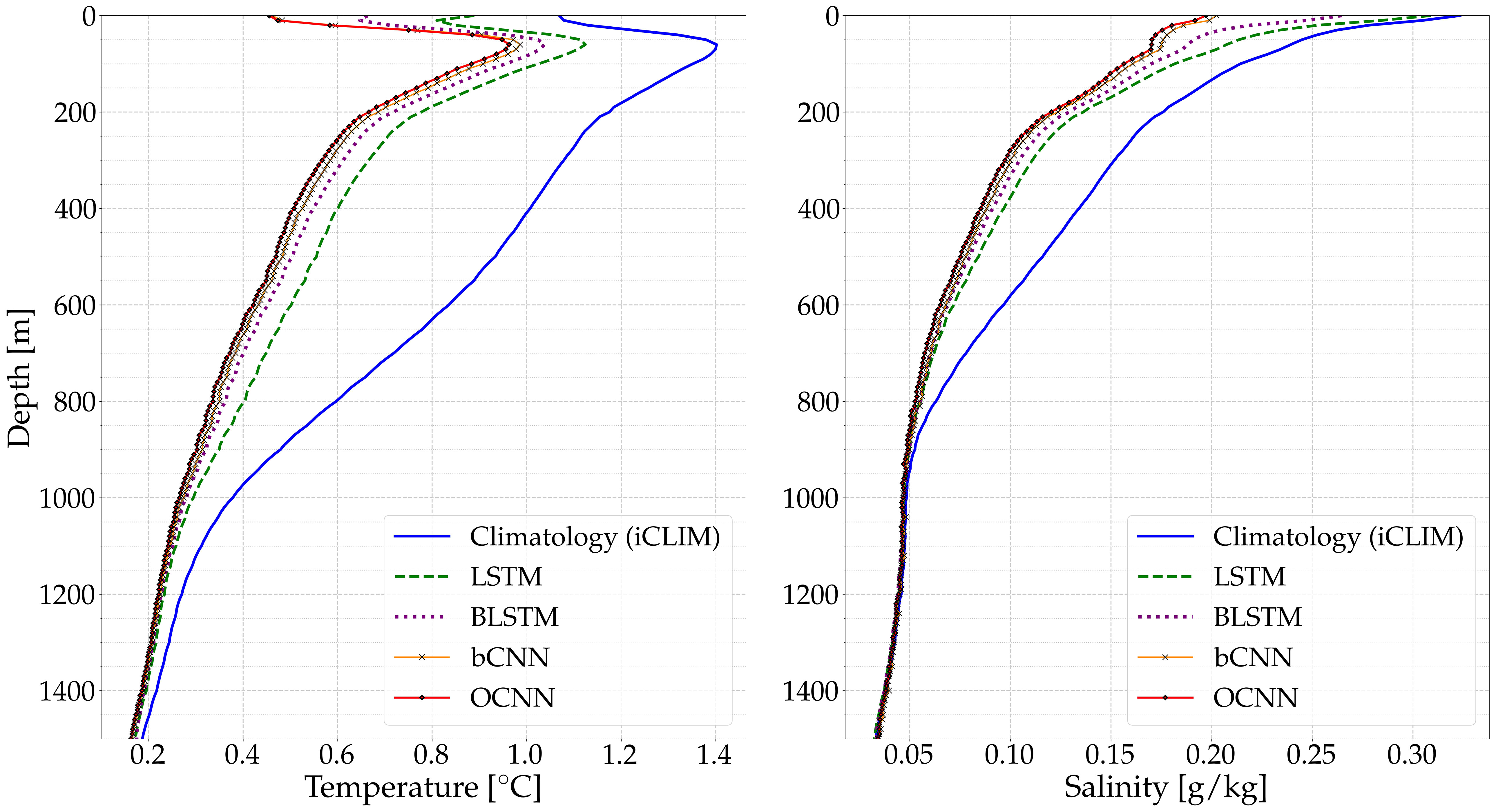
Figure 3 Vertical RMSE profiles for each model from the surface down to 1500 m at 10 m intervals of temperature (left) and salinity (right).

In all evaluated models, the most significant temperature errors were observed at depths of 60-90m, while salinity errors were primarily near the surface. The highest error in temperature appears to be located at the generally accepted mixed layer depth for the study area. Since temperature and salinity gradients are stronger in this part of the water column, even small displacements in the depth used for reconstruction may yield large errors. A mechanism that supports the hypothesis that regions with high variability are those with larger RMSE. The relatively larger RMSE values for salinity estimates at the surface may to some extent have been a consequence of the discrepancies between satellite and in situ salinity measurements. As previously outlined, these discrepancies can be attributed to the interpolation of the coarse-resolution satellite product and the influence of short-term or small-scale in situ fluctuations. Therefore, the effects of the mixed layer depth are less conspicuous in the RMSE values for salinity.

At low variability depth regions (approx. 900 m depth) there were no differences between the models, and for salinity, the iCLIM demonstrates similar levels of error to the neural network models. This suggests that salinity values in this region are not strongly influenced by surface variables, and that the similar estimates are provided by the iCLIM.

An assessment of the spatial distribution of the errors was obtained by calculating the average RMSE in the first 200m for the entire test set (Figure 4). The largest errors were associated mostly with highly dynamic regions in the western boundary currents (Gulf Stream, Brazil Current) and the eddy dynamics driven by the Agulhas Current. Equatorial regions also showed relatively large errors, likely linked to the intensity of the ocean currents and mixed layer dynamics in the area. For salinity, the areas with the largest errors roughly coincided with regions of highest variability in data ((Figure 1B).

FIGURE 4

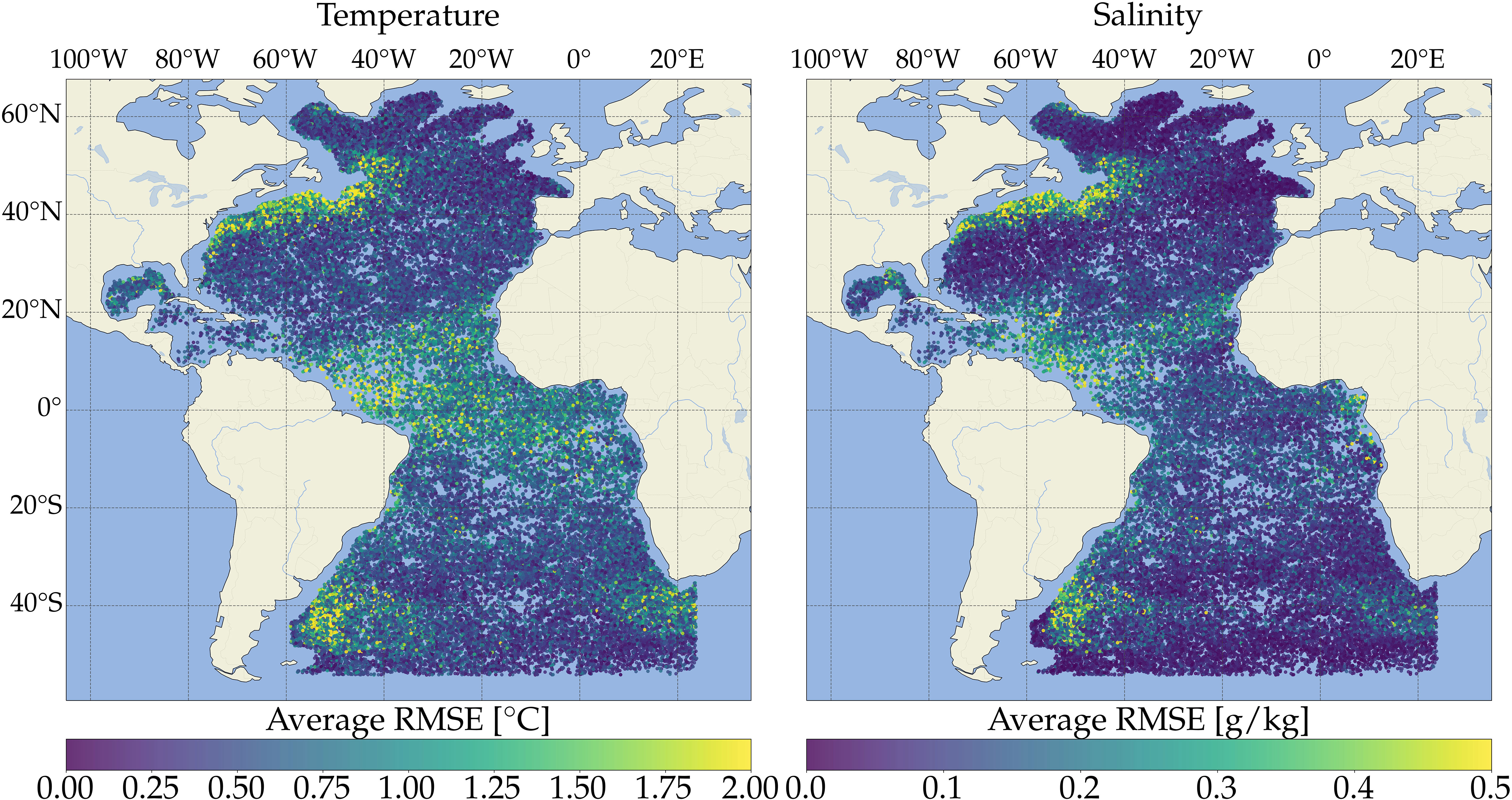
Figure 4 Spatial map of RMSE values in the top 200m between the OCNN predictions and observed test data.

3.2 Feature importance and model sensitivity

The OCNN model was tested under different configurations with various input and output variables (See Appendix 6.4, Table S1). From several tests, we found that the optimal input combination for temperature and salinity profile reconstruction consists of: sea surface temperature, salinity, density, sum of wind speeds, and absolute dynamic topography (SST, SSS, DOS, SSW_sum, ADT), the corresponding anomalies SSTA, SSSA, ADTA, DOSA, SSWA_sum, error estimates of SST and SSS (SST_error, SSS_error), and finally lat, lon and day of year (DOY). It should be noted that the deviations from the climatological mean are included in original measurements as well as in the corresponding anomalies, but the original measurements were considered useful as they provided contextual reference points for different regions. The use of error estimates of other input variables such as ADT and SSW were considered but appeared to have little to no significance on the reconstruction capabilities.

For the reconstruction of temperature, also modelling several outputs of full profiles of temperature, salinity, steric height (SH), density (D), thermal expansion coefficient (TC), and their respective anomalies yielded better results. Although the above inputs improved also the reconstructions of salinity, the best results for the reconstruction of this variable were obtained by modeling a singular output, the subsurface salinity anomalies (SA). For that reason, two separate models were used for temperature and salinity reconstructions. Using these combinations of inputs and outputs, the average reconstruction errors of temperature and salinity were reduced by 5.3% and 5.5% respectively.

An analysis of the relative importance of those inputs using Shapley values demonstrated that sea surface temperature, SST, and surface density, DOS, are on average the most important for the reconstruction of the profiles of temperature and salinity (Figure 5). However, the relative Shapley values indicate relative importance of inputs rather than reconstruction accuracy, which as seen in Figure 3 resembles the climatological averages for all models at depth greater than 1000m. Thus, this method does not necessarily suggest causation between surface and subsurface properties, but a network may use secondary information such as leveraging the inputs as geographical reference points. Predictions of temperature in the first 200m depended rather strongly on the values of surface temperature anomaly, SSTA. Similarly, the surface salinity anomaly (SSTA) had high relative importance for the prediction of salinity in the surface layers. Between depths of 100-600m, the absolute dynamic topography and corresponding anomaly (ADT and ADTA, respectively) exhibited a considerable increase in relative importance for both salinity and, notably, temperature reconstructions. This is not surprising as ADT values are commonly linked to the density structure of the water column. Within the same vertical range, geographical position (mainly latitudes, and to a lesser extent longitudes) had a significant impact on model performances for both temperature and salinity.

FIGURE 5

Figure 5 The mean magnitude of Shapley values computed using SHAP of each input in the CNN model as a function of depth. The relative importance is scaled between 0-1.

Random white noise was introduced on each variable to test sensitivity of the reconstructed profiles to input. By randomly selecting a ±5% deviation from a uniform distribution, RMSE values were then calculated and compared with the unperturbed case. The averaged (over the depth) error increased significantly for certain variables (SST, SSS, ADT, and associated anomalies) and generally reconstruction in salinity appeared to be the most sensitive to changes (Figure 6). We noted that errors in reconstructions were considerably larger when altering only the variable but not the corresponding anomaly. In these scenarios, the increase in error propagated with the entire depth range, with the highest values at maximum depths. This is in particular the case for salinity and density, and it indicates that the model is highly dependent on the coherence between the original and anomaly values of a variable. An exception is the ADT where varying the original and anomaly values together has a larger effect than separately. One reason for this may be that the anomaly fields for ADT are defined with respect to steric height computed from values of temperature and salinity, and not direct in situ measurements of the topography. Similarly, as indicated by the Shapley values, latitudes and longitudes have some effects on the model performance for both temperature and salinity. In particular, latitude is important for temperature reconstructions within a specific depth range, i.e., 50-300 m.

FIGURE 6

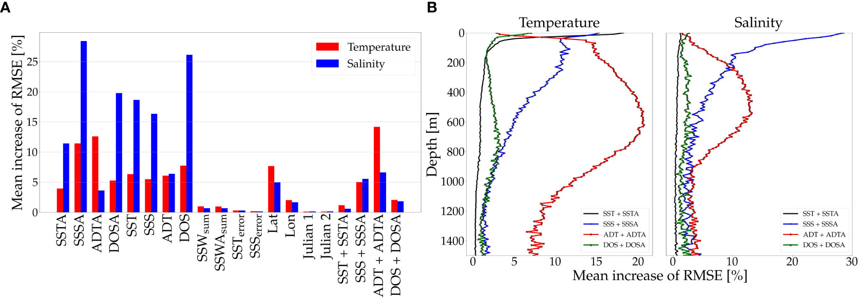
Figure 6 A random noise was repetitively added to each input individually, generating a series of new RMSE depth profiles. The mean percentage decrease of these RMSE profiles is here compared to the original test scores (A). The mean percentage decrease of RMSE in depth for the four last columns of the histogram (B). The noises were randomly selected from uniform distributions with ±5% of the signal variance of each variable.

The mean percentage decrease of the RMSE at various depths for input variations of SST, SSS, ADT, and DOS and their respective anomalies simultaneously are displayed in Figure 6. It is apparent that perturbations in the SST and the SSS have the largest impact in the uppermost layers for the reconstruction of their respective subsurface variables ST and SS. Changes of SST by 0 − 5% correspond to an average decrease in reconstruction performance of temperature at the surface by almost 20%, and changes of SSS impact the surface reconstructions of salinity by 30%. Perturbations in the input of SST and SSS lead to significant amplifications of errors in the upper ocean layers, while changes in ADT result in error propagation to larger depths as also indicated by the Shapley values. In particular, these effects are noticeable at depths ranging from 200m to 1000m, where the average decrease in performance is 10-20%. As previously mentioned, this can be understood as the surface topography being governed by a summation of steric changes, due to variations in temperature and salinity that occur throughout the entire vertical profile, see (Jones et al., 1998; Guinehut et al., 2012; Zhang et al., 2012).

3.3 Improvements compared to climatological data

To assess the advantages of convolution neural network relative to traditional methods, we compared the results from the OCNN using the input and output combination from the previous section with iCLIM values in different regions. Generally, the OCNN had greater accuracy of iCLIM across the entire water column when averaged over the model domain, with the difference being minimal at greater depths where conditions are mostly stable. While the OCNN performances generally were better closer to the surface and especially around the base of the surface mixed layer (cf. Figure 3).

These results are confirmed when performances across different regions in the Atlantic Ocean (Figure 4) were analyzed. Reconstructions of both temperature and salinity using the OCNN had higher accuracy than iCLIM in regions at higher latitudes, while in tropical and equatorial regions the difference in performance between the two models was reduced (Figure 7). This is because temperate and polar regions have larger variability in the ocean conditions than tropical regions, hence, as expected, the simple interpolation of climatological profiles did not provide good reconstruction values when compared to the OCNN. The improvement in reconstruction accuracy is similar for temperature and salinity across the different regions, although for temperature the OCNN showed better performances. On the contrary, in Equatorial regions, the OCNN can occasionally have poorer performances than iCLIM (Figure 7). It should be noted, however, that in these regions only limited training and testing data were available, so that accurate comparisons should are dubious.

FIGURE 7

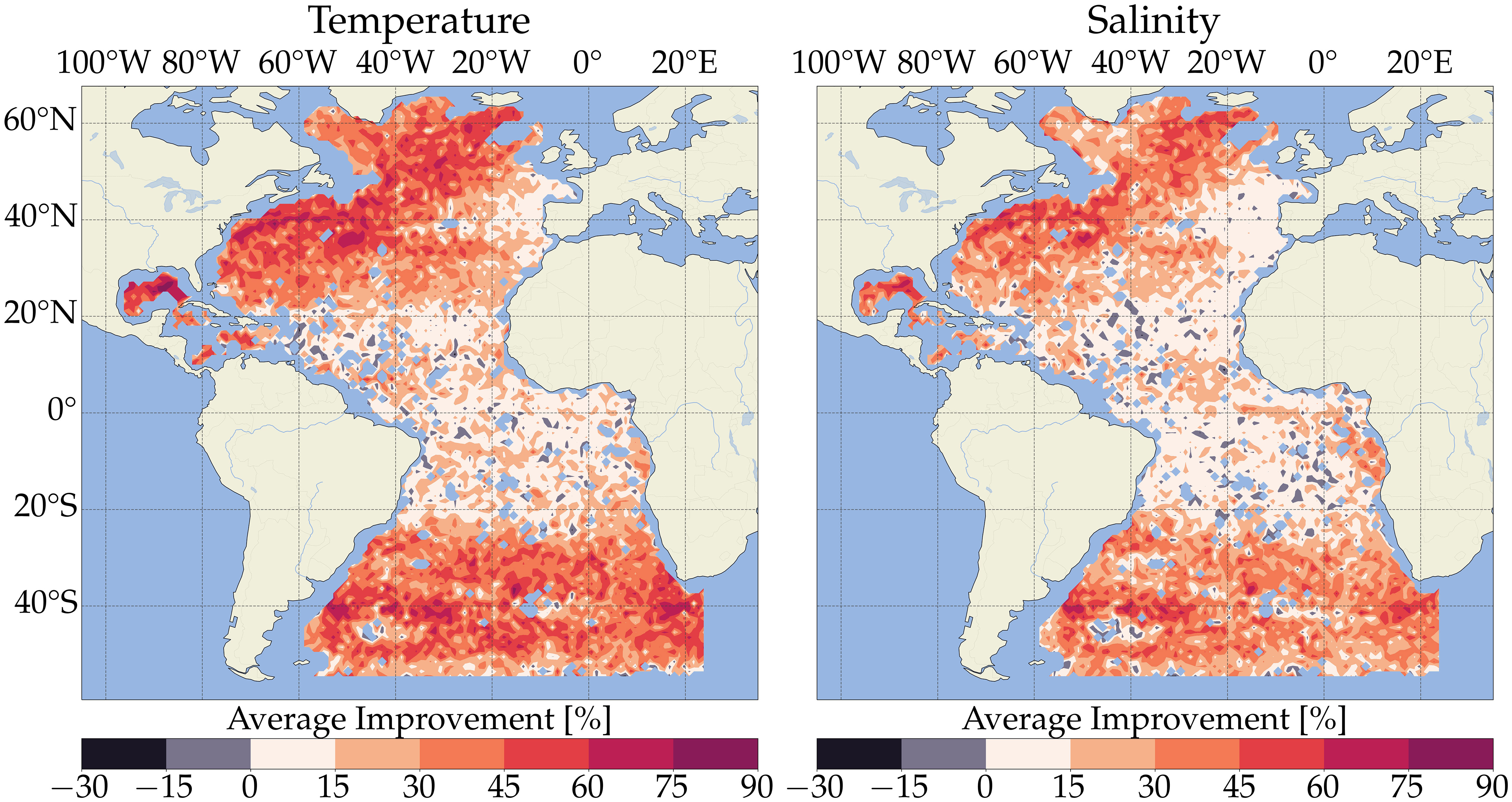
Figure 7 Test scores improvements comparing iCLIM to the OCNN estimates.

With regard to specific regions (see Figure 1B) there were substantial differences in the accuracy of the OCNN respect to iCLIM (see Table 4). The OCNN had >50% improvement in reconstructions for temperature, and approximately 40% for salinity, in regions A, D, and E which are the most dynamic among those selected. While in region C a smaller improvement in temperature and no improvement in salinity were observed. The comparison with the mean RMSE values from Table 3 indicates a notable reduction in the overall mean RMSE values across the Atlantic for the OCNN. This improvement is as a result of using the model with the optimal input-output combination. The high RMSE values for surface salinity seen in Figure 3 were not observed uniformly across the Atlantic. They were particularly high and frequent in dynamic areas such as the Gulf Stream and near river outlets, thereby increasing the overall RMSE. The vertical RMSE profiles varied considerably for both temperature and salinity across different study regions (A–E), and only in Region B, corresponding to the Amazon River outlet, were the salinity RMSE values largest at the surface (See Appendix 6.3, Figure S3).

TABLE 4

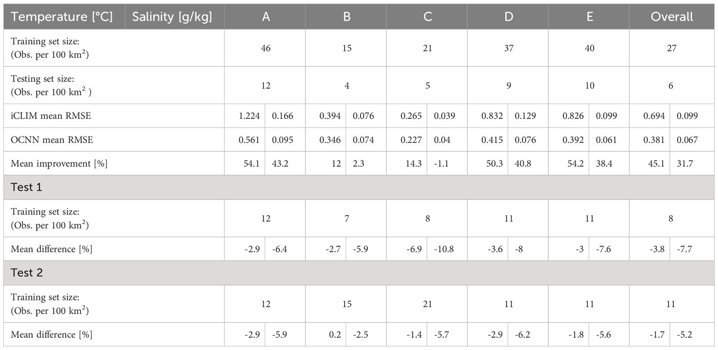
Table 4 Reconstruction results in selected regions defined in section 2.3.

By removing observed profiles from those regions we tested the effects of training on the accuracy of the model. Specifically, we tested two cases (Test 1 and Test 2 in Table 4). In the first case profiles were removed randomly to obtain a more uniform distribution of observations in all regions across the whole Atlantic. In the second case (Test 2) observations were not removed from regions with few observations (i.e., B, C, 100% retain of the original data). In Test 1 the training set was reduced by 68% with a maximum of 12 profiles per 100 km² across all regions. Similar reduction was used in Test 2 but no observations were removed from regions B and C, which had then respectively, 15 and 21 observations per 100 km².

The mean improvement is measured with respect to the interpolated climatological averages (iCLIM). Temperature and salinity are measured in °C and [g/kg] respectively. Two tests were performed reducing the size of the training set by about 70%, in Test 1 across all regions while in Test 2 no profiles were removed from regions B and C. The calculated mean difference is relative to the same model trained on the full data set.

For both temperature and salinity profiles, the reconstruction accuracy decreased proportionally to the reduction of training data (see Table 4). Calculating the mean difference across the entire Atlantic with respect to a model trained on the full data set, we obtain that reconstructions of salinity deteriorate more than those for temperature (overall mean difference -7.7% and -3.8, respectively, Test 1).

When training profiles are preserved in some regions (Test 2), the reconstruction accuracy of temperature in Region B remained relatively stable, while slightly decreasing in Region C. However, there was still a considerable decline in the performance of salinity reconstructions, particularly in Region B. This indicates that the use of training information of a non-local character, coming from regions other than B, may be useful for improving salinity reconstruction. This notion is further supported when comparing the two tests, as improvements were observed not only in Region B and C but also in other regions (i.e., A, D, E).

4 Discussion

Prior work reconstructed the subsurface ocean structure using LSTMs by considering profiles as time series (Buongiorno Nardelli, 2020; Su et al., 2021b). In this study we implement different LSTM and CNN architectures, and illustrate that CNNs have lower reconstruction error than that of LSTMs for all depths. Furthermore, we show the importance of tuning the structure and parameters of a CNN to obtain improved reconstruction estimates and evaluate the importance of different parameters (type of variables and training size) in improving the performances.

Previous studies have shown that sea surface height and temperature as input features combined with additional variables, such as wind stress, can improve the reconstruction of ocean state variables (Ali et al., 2004; Jeong et al., 2019; Lu et al., 2019). However, a systematic analysis of the impact of different input-output feature combinations on reconstruction performance was lacking. This paper presents such systematic analysis performing different tests of input-output variations with the same CNN model. Our findings demonstrate that incorporating variables such as surface density (DOS) and sum of wind speeds (SSW_sum) improved the reconstruction performance. Moreover, inclusion of both the measured values and their anomalies as input variables further improved reconstructions for both temperature and salinity. For temperature reconstructions, constructing a model that includes additional outputs, such as the measured profiles, their respective anomalies, and profiles of density and steric height, showed even better results. Conversely, for salinity reconstructions, using only profiles of salinity anomalies (SA) yields better results.

Globally, the addition of all input features presented in Section 3.2 provides on average 5% improvements in reconstructions, i.e., reduces reconstruction RMSE for both temperature and salinity. However, at local scales the impact of additional input features is greater, particularly for salinity and in regions with highly variable conditions. In regions such as the Gulf Stream and Agulhas Current, wind plays an important role, and adding SSW_sumalong with the other additional inputs leads to almost a 10% decrease in mean RMSE for salinity reconstructions. In our study, we find that the incorporation of certain input features can increase RMSE. For instance, introducing geostrophic currents (UGOS/VGOS) and of wind speed components (USSW/VSSW) has a negative impact on the reconstruction performance. The cause of this could be attributed to errors in spatial or temporal interpolation, lag effects from surface changes to changes in the deeper ocean, or a lack of physical coupling between surface input and subsurface output features.

Many studies have focused on exploring different model designs and deep learning architectures, while an in-depth analyses of the importance of different input-output variables has only recently received attention (Pauthenet et al., 2022). In this study, we have demonstrated that analyzing feature importance and input sensitivity can enhance our understanding of how neural networks reconstruct oceanographic features. Furthermore, this approach can inform the design of observational networks by identifying variables that require more accurate information to improve reconstruction performance. The analysis using Shapley values revealed that sea surface temperature and salinity, as well as their anomalies, played a crucial role in estimating the respective subsurface variables. For deeper layers, the surface topography (ADT) and, to some extent, latitude had relatively higher importance in reconstructing both variables. Links between these physical variables have been demonstrated in previous studies (Jones et al., 1998; Guinehut et al., 2012; Liu et al., 2017). However, the surface values of SST and SSD appeared to have disproportionate importance for the OCNN, particularly at deeper layers. This may be an indication that the network is using these variables as locational proxies in its reconstructions, rather than as indicators of deeper ocean physical variables. While the feature importance analyses provides a clear overview about the relative weight of different inputs in profiles reconstruction, it is important to underline that those relationships do not necessarily indicate causation in the physical relations between sea surface and subsurface properties and conditions. However, several studies (Lapeyre and Klein, 2006; Liu et al., 2017; Chen et al., 2020) indicate, that some dynamics down to depths of 1000m may be captured by reconstruction based on that surface temperature, height, and density fields. This suggests that the high relative importance may indeed reflect links between sea surface and subsurface conditions and properties to depths of 1000m. Reconstructions for deeper ocean layers appear to deteriorate rapidly, which is consistent with the findings of this study, and one should view the high relative importance with caution.

The accuracy of OCNN is influenced by both regional and profile-based variability. Errors in temperature reconstruction were higher at the base of the mixed-layer, while for salinity the worst performance is at surface. This is partially because small perturbations on SSS had large impacts on the reconstructions of salinity profiles (Section 3.2). A systematic perturbation of SSS inputs within 0 − 5% range, showed drops in model accuracy by an average 30% for the surface values, and an average of 6% for the entire profile. Hence, since discrepancies between in situ and satellite surface measurements frequently exceed ±5%, the low accuracy of OCNN at the surface could be expected. Indeed by substituting surface satellite inputs of salinity directly with in situ measurements (data not shown) we obtained major improvements in the accuracy of OCNN not only for surface estimates, but for reconstructions in the first 70m. This result is consistent with previous findings that employed spatial upsampling of salinity data using satellite SST differences to shape and constrain surface patterns (Buongiorno Nardelli, 2020).

In general, RMSE values indicate that salinity estimates using neural network-based models are less accurate than temperature estimates and show smaller improvements (45% for temperature and 32% for salinity) when compared to profiles obtained using iCLIM. A potential reason for this may be that relationships between surface and subsurface conditions, such as the connection between altimeter measurements and steric contributions to surface height, are only able to explain a limited portion of the variability in the salinity signal, as observed in earlier studies [e.g., (Guinehut et al., 2012)]. Specifically, in the ocean depths beyond 1000 meters, all models yielded identical RMSE results. One possible explanation for this might be the complete disconnection between surface variables and the deep ocean dynamics. This notion is further supported by the negligible impact of introducing random white noise to the inputs on salinity predictions below 900 meters, see Section 3.2.

The size of the training set has a considerable impact on the performance of the OCNN reconstructions. When the training set size is reduced by about 70%, the overall RMSE scores display a decrease of 3.8% and 7.7% for temperature and salinity, respectively. These impacts seem to have both local and non-local implications, as retaining training examples in specific regions affects the RMSE outcomes throughout the Atlantic, even though the impacts are more noticeable in those regions. Despite the non-uniform spatial reduction in training data and the preservation of more data in regions with lower observation density, the most substantial effects on salinity reconstructions are observed in these regions, with some experiencing RMSE reductions of approximately 11%. This has consequences for the sampling strategies of in situ measurements, since a minimum number of samples across various Atlantic regions is necessary for robust reconstructions. However, this research suggests that neural network-based models also learn patterns and dynamics that can be utilized for reconstructions in other regions. Further research could identify regions that provide relatively more information, both local and non-local, compared to regions where only a few training observations are sufficient to generate robust estimates. Strategies for future deployments of Argo profiles may benefit greatly from such analysis.

As a result of the criteria for in situ measurements in this study, about 50% of the available profiles in the Atlantic were discarded. A large portion of these samples could be suitable for similar studies focusing on reconstructing hydrographic profiles in shallower waters. Using these profiles would considerably increase the number of training examples, offering both local and non-local information. Specifically for salinity reconstruction, having more training examples greatly influenced the results. Furthermore, since the reconstruction of salinity did not outperform iCLIM in regions deeper than 900 meters, it would be beneficial to include additional shallower profiles.

Using the optimal input-output variable combination from the current study, future research could explore local spatial and temporal dependencies. One potential approach would be to construct a 3D matrix for each input feature, utilizing a 2D time series of spatial maps. The height and width of the matrix would correspond to the spatial signature of the adjacent surface values, while the depth of the matrix would represent the temporal change. The CNN model and its architecture should be adapted accordingly to this input, i.e., changing from one-dimensional to two- or three-dimensional convolutional layers. Prior studies (Su et al., 2021b; Su et al., 2022; Sun et al., 2022) have used spatial and temporal dimensions in a more explicit manner than in this study. However, much research is still required to fully evaluate and understand the dominant patterns and modes within the surface data.

We found that reconstruction errors are reduced when more profiles are used for training, but we did not analyze the epistemic vs the aleatoric uncertainty. For this purpose, the CNN should be made fully Bayesian so that it becomes possible to estimate both the expected values, corresponding to the deterministic reconstructions and their data and model uncertainty. Equipped with a measure of data uncertainty, the model would make it easier to determine the need for additional Argo floats in specific regions.

5 Conclusion

In this study, we reconstruct the salinity and temperature vertical profiles of the Atlantic Ocean down to a depth of 1500 m using a one-dimensional convolution neural network. We demonstrate that the effectiveness of neural network-based methods for combining accurate but sparse in situ profiles with remotely-sensed surface measurements can vary significantly depending on the specific algorithm employed. Our study resulted in the development of an optimized convolutional neural network (OCNN), which showed superior performance compared to other neural network approaches such as LSTM, a simpler version of the CNN (bCNN), and reconstructions based on climatological values.

The non-uniform spatial distribution of errors showed lower accuracy associated mostly with highly dynamic regions in the western boundary currents (Gulf Stream, Brazil Current) and in the Agulhas Current. The central challenge in reconstructing temperature residuals lies in accurately estimating values within the 60-90 meter depth range at the base of the upper mixed layer. For salinity reconstructions, discrepancies between satellite surface measurements and in situ observations appeared to have greater influence on the performance, surpassing the influence of near-surface variability.

Our research revealed that incorporating additional and specific combinations of inputs and outputs into the networks resulted in even greater improvement in reconstruction performance. The distribution of

relative importance between the inputs varied with depth, where some inputs were central to the upper and mixed layer depth (0-200m) such as surface anomalies of temperature and salinity (SSTA, SSSA), and to some extent the wind speed. Other variables such as the measured values of surface temperature and salinity (SST, SSS), and values of ADT had greater importance at depths of range 200-1000m.

We demonstrate that a decrease in the spatial density of in situ profiles across the Atlantic results in a reduced reconstruction performance in high variability regions, such as the Gulf Stream, and an even greater decline in low variability regions. However, preserving training observations in specific regions, not only leads to local reconstruction improvements in those regions, but also enhances overall performance across the Atlantic. This suggests that a minimum number of training examples is necessary across various Atlantic regions, while much local information can be extrapolated to other locations. The effects of reduced training data are particularly noticeable for salinity reconstructions. With the original number of in situ observations in low variability regions, the areas remain sparsely sampled, and the predictions show improvements although minimal compared to climatological averages. Additional observations in these regions could further increase the gap from estimates based on climatological averages.

This research demonstrates that convolutional neural network-based architectures such as the OCNN for reconstruction of subsurface ocean structure yield promising outcomes. By utilizing and further advancing this framework, more precise insights into ocean structure can be acquired, leading to a better comprehension of the Earth System and shifts in its dynamics.

Data availability statement

The raw data supporting the conclusions of this article will be made available by the authors, without undue reservation.

Author contributions

All authors contributed to the development of the concepts and methods presented in this paper, which ultimately shaped the problem statement and results. PS was responsible for curating the data and applying statistical and computational techniques for the analysis. Additionally, PS implemented supplementary algorithms, visualized the data, and wrote the initial draft. KS contributed valuable ideas for the model setup and the execution of the algorithms. BN offered expertise and insights in the scientific domain and introduced the team to widely-used frameworks within the field. PM, FR, AsC, AnC, and MS contributed by supplying study materials and data resources, validating and verifying the results, and offering ideas during the implementation process. PM served as the primary supervisor and actively participated in overseeing the project administration. All authors contributed to the article and approved the submitted version.

Funding

This article is delivered under the MISSION ATLANTIC project funded by the European Union’s Horizon 2020 Research and Innovation Program under grant agreement No. 639 862428. The work of PS and PM was partially supported by BRIDGE-BS project funded by the European Union’s Horizon 2020 Research and Innovation Program under grant agreement No. 101000240.

Conflict of interest

The authors declare that the research was conducted in the absence of any commercial or financial relationships that could be construed as a potential conflict of interest.

Publisher’s note

All claims expressed in this article are solely those of the authors and do not necessarily represent those of their affiliated organizations, or those of the publisher, the editors and the reviewers. Any product that may be evaluated in this article, or claim that may be made by its manufacturer, is not guaranteed or endorsed by the publisher.

Supplementary material

The Supplementary Material for this article can be found online at: https://www.frontiersin.org/articles/10.3389/fmars.2023.1218514/full#supplementary-material

Footnotes

1. ^ https://marine.copernicus.eu/.
2. ^ https://github.com/bbuong/3Drec.

References

Ali M., Swain D., Weller R. (2004). Estimation of ocean subsurface thermal structure from surface parameters: A neural network approach. Geophys. Res. Lett. 31, L20308. doi: 10.1029/2004GL021192

CrossRef Full Text | Google Scholar

Amani M., Ghorbanian A., Asgarimehr M., Yekkehkhany B., Moghimi A., Jin S., et al. (2022). Remote sensing systems for ocean: A review (part 1: Passive systems). IEEE J. Selected Topics Appl. Earth Observations Remote Sens. 15, 210–234. doi: 10.1109/JSTARS.2021.3130789

CrossRef Full Text | Google Scholar

Bindoff N., Cheung W., Arístegui J., Guinder V., Hallberg R., Hilmi N., et al. (2019). Changing Ocean, Marine Ecosystems, and Dependent Communities. In: IPCC Special Report on the Ocean and Cryosphere in a Changing Climate [Pörtner H.-O., Roberts D. C., Masson-Delmotte V., Zhai P., Tignor M., Poloczanska E., et al (eds.)]. Cambridge University Press, Cambridge, UK and New York, NY, USA, pp. 447–587. doi: 10.1017/9781009157964.007

CrossRef Full Text | Google Scholar

Bourassa M. A., Romero R., Smith S. R., O’Brien J. J. (2005). A new fsu winds climatology. J. Climate 18, 3686–3698. doi: 10.1175/JCLI3487.1

CrossRef Full Text | Google Scholar

Boutin J., Reul N., Köhler J., Martin A., Catany R., Guimbard S., et al. (2021). Satellite-based sea surface salinity designed for ocean and climate studies. J. Geophysical Research: Oceans 126, e2021JC017676. doi: 10.1029/2021JC017676

CrossRef Full Text | Google Scholar

Buongiorno Nardelli B. (2020). A deep learning network to retrieve ocean hydrographic profiles from combined satellite and in situ measurements. Remote Sens. 12. doi: 10.3390/RS12193151

CrossRef Full Text | Google Scholar

Buongiorno Nardelli B., Cavalieri O., Rio M.-H., Santoleri R. (2006). Subsurface geostrophic velocities inference from altimeter data: Application to the sicily channel (mediterranean sea). J. Geophysical Research: Oceans 111. doi: 10.1029/2005JC003191

CrossRef Full Text | Google Scholar

Buongiorno Nardelli B., Pisano A., Sammartino M. (2022). Quality information document: For multi observation global ocean sea surface salinity and sea surface density product MULTIOBS_GLO_PHY_ S_SURFACE_MYNRT_015_013. Copernicus Marine Service, ref. CMEMS-MOB-QUID-015-013, August 2022, v1.2, pp.24. Available at: https://catalogue.marine.copernicus.eu/documents/QUID/CMEMS-MOB-QUID-015-013.pdf.

Google Scholar

Carnes M. R., Mitchell J. L., de Witt P. W. (1990). Synthetic temperature profiles derived from geosat altimetry: Comparison with air-dropped expendable bathythermograph profiles. J. Geophysical Research: Oceans 95, 17979–17992. doi: 10.1029/JC095iC10p17979

CrossRef Full Text | Google Scholar

Carnes M. R., Teague W. J., Mitchell J. L. (1994). Inference of subsurface thermohaline structure from fields measurable by satellite. J. Atmos. Ocean Technol. 11, 551–566. doi: 10.1175/1520-0426(1994)011⟨0551:IOSTSF⟩2.0.CO;2

CrossRef Full Text | Google Scholar

Castro S. L., Wick G. A., Jackson D. L., Emery W. J. (2008). Error characterization of infrared and microwave satellite sea surface temperature products for merging and analysis. J. Geophysical Research: Oceans 113, C03010. doi: 10.1029/2006JC003829

CrossRef Full Text | Google Scholar

Chen Z., Wang X., Liu L. (2020). Reconstruction of three-dimensional ocean structure from sea surface data: An application of isqg method in the southwest Indian ocean. J. Geophysical Research: Oceans 125, e2020JC016351. doi: 10.1029/2020JC016351

CrossRef Full Text | Google Scholar

Cheney R. E. (1982). Comparison data for seasat altimetry in the western north atlantic. J. Geophysical Research: Oceans 87, 3247–3253. doi: 10.1029/JC087iC05p03247

CrossRef Full Text | Google Scholar

Fox D., Barron C., Carnes M., Lee C. (2002). The modular ocean data assimilation system (modas). J. Atmospheric Oceanic Technol. - J. ATMOS OCEAN Technol. 19, 240–252. doi: 10.1175/1520-0426(2002)019⟨0240:TMODAS⟩2.0.CO;2

CrossRef Full Text | Google Scholar

Graves A., Schmidhuber J. (2005). Framewise phoneme classification with bidirectional lstm and other neural network architectures. Neural Networks 18, 602–610. doi: 10.1016/j.neunet.2005.06.042

PubMed Abstract | CrossRef Full Text | Google Scholar

Guinehut S., Dhomps A.-L., Le Traon P. Y., Gilles L. (2012). High resolution 3-d temperature and salinity fields derived from in situ and satellite observations. Ocean Sci. 8, 845–857. doi: 10.5194/os-8-845-2012

CrossRef Full Text | Google Scholar

Han M., Feng Y., Zhao X., Sun C., Hong F., Liu C. (2019). A convolutional neural network using surface data to predict subsurface temperatures in the pacific ocean. IEEE Access 7, 172816–172829. doi: 10.1109/ACCESS.2019.2955957

CrossRef Full Text | Google Scholar

Jeong Y., Hwang J., Park J., Jang C., Jo Y.-H. (2019). Reconstructed 3-d ocean temperature derived from remotely sensed sea surface measurements for mixed layer depth analysis. Remote Sens. 11, 3018. doi: 10.3390/rs11243018

CrossRef Full Text | Google Scholar

Jones M. S., Allen M., Guymer T., Saunders M. (1998). Correlations between altimetric sea surface height and radiometric sea surface temperature in the south atlantic. J. Geophysical Research: Oceans 103, 8073–8087. doi: 10.1029/97JC02177

CrossRef Full Text | Google Scholar

Kao T. W. (1987). The gulf stream and its frontal structure: a quantitative representation. J. Phys. Oceanogr. 17, 123–133.

Google Scholar

Khedouri E., Szczechowski C., Cheney R. (1983). “Potential oceanographic applications of satellite altimetry for inferring subsurface thermal structure,” in Proceedings OCEANS ’83. (San Francisco, CA, USA: IEEE) 274–280. doi: 10.1109/OCEANS.1983.1152138

CrossRef Full Text | Google Scholar

Kingma D. P., Ba J. (2014). Adam: A method for stochastic optimization. arXiv preprint arXiv, 1412.6980. doi: 10.48550/ARXIV.1412.6980

CrossRef Full Text | Google Scholar

Kiranyaz S., Avci O., Abdeljaber O., Ince T., Gabbouj M., Inman D. J. (2021). 1d convolutional neural networks and applications: A survey. Mech. Syst. Signal Process. 151, 107398. doi: 10.1016/j.ymssp.2020.107398

CrossRef Full Text | Google Scholar

Klambauer G., Unterthiner T., Mayr A., Hochreiter S. (2017). “Self-norMalizing neural networks,” in Advances in neural information processing systems, vol. 30 . Eds. Guyon I., Luxburg U. V., Bengio S., Wallach H., Fergus R., Vishwanathan S., Garnett R. (Long Beach, CA: Curran Associates, Inc), 971–980.

Google Scholar

Lapeyre G., Klein P. (2006). Dynamics of the upper oceanic layers in terms of surface quasigeostrophy theory. J. Phys. Oceanogr. 36, 165–176. doi: 10.1175/JPO2840.1

CrossRef Full Text | Google Scholar

Liu L., Peng S., Huang R. X. (2017). Reconstruction of ocean’s interior from observed sea surface information. J. Geophysical Research: Oceans 122, 1042–1056. doi: 10.1002/2016JC011927

CrossRef Full Text | Google Scholar

Locarnini R., Mishonov A., Baranova O., Boyer T., Zweng M., Garcia H., et al. (2019). World ocean atlas 2018, Volume 1: Temperature. A. Mishonov, Technical Editor. In Observing the Oceans in the 21st Century (C.J. Koblinsky and N.R. Smith).(NOAA Atlas NESDIS 81), 52pp.

Google Scholar

Loshchilov I., Hutter F. (2017). SGDR: Stochastic Gradient Descent with Warm Restarts. Preprint. arXiv:1608.03983 Cs Math.

Google Scholar

Lu W., Su H., Yang X., Yan X.-H. (2019). Subsurface temperature estimation from remote sensing data using a clustering-neural network method. Remote Sens. Environ. 229, 213–222. doi: 10.1016/j.rse.2019.04.009

CrossRef Full Text | Google Scholar

Lundberg S. M., Lee S.-I. (2017). A unified approach to interpreting model predictions. Proceedings of the 31st International Conference on Neural Information Processing Systems, Long Beach, CA, December 2017, NIPS’17. NY, USA: Red Hook Curran Associates Inc., 4765–4774. doi: 10.48550/ARXIV.1705.07874

CrossRef Full Text | Google Scholar

McLaren E., Roberts-Jones J., Martin M., Mao C., Good S. (2016). Global ocean ostia near real time level 4 sea surface temperature product. SST-GLO-SST-L4-NRT-OBSERVATIONS-010-001, EU Copernicus Marine Service. 2016. Available online: https://catalogue.marine.copernicus.eu/documents/QUID/CMEMS-SST-QUID-010-001.pdf.

PubMed Abstract | Google Scholar

Meng L., Yan X.-H. (2022). Remote sensing for subsurface and deeper oceans: An overview and a future outlook. IEEE Geosci. Remote Sens. Magazine. 10, 72–92. doi: 10.1109/MGRS.2022.3184951

CrossRef Full Text | Google Scholar

Moltmann T., Turton J., Zhang H.-M., Nolan G., Gouldman C., Griesbauer L., et al. (2019). A global ocean observing system (goos), delivered through enhanced collaboration across regions, communities, and new technologies. Front. Mar. Sci. 6, 291. doi: 10.3389/fmars.2019.00291

CrossRef Full Text | Google Scholar

Nardelli B., Guinehut S., Verbrugge N., Cotroneo Y., Zambianchi E., Iudicone D. (2017). Southern ocean mixed-layer seasonal and interannual variations from combined satellite and in situ data. J. Geophysical Research: Oceans 122, 10042–10060. doi: 10.1002/2017JC013314

CrossRef Full Text | Google Scholar

Nardelli B., Santoleri R. (2005). Methods for the reconstruction of vertical profiles from surface data: Multivariate analyses, residual gem, and variable temporal signals in the north pacific ocean. J. Atmos. Ocean Technol. 22, 1762–1781. doi: 10.1175/JTECH1792.1

CrossRef Full Text | Google Scholar

Pauthenet E., Bachelot L., Balem K., Maze G., Tréguier A.-M., Roquet F., et al. (2022). Fourdimensional temperature, salinity and mixed-layer depth in the gulf stream, reconstructed from remotesensing and in situ observations with neural networks. Ocean Sci. 18, 1221–1244. doi: 10.5194/os-18-1221-2022

CrossRef Full Text | Google Scholar

Roemmich D., Boebel O., Desaubies Y., Freeland H., Kim K., King B., et al. (2001). “Argo: The global array of profiling floats,” in Observing the oceans in the 21st century.

Google Scholar

Sørensen K. A., Heiselberg P., Heiselberg H. (2022). Probabilistic maritime trajectory prediction in complex scenarios using deep learning. Sensors 22, 2058. doi: 10.3390/s22052058

PubMed Abstract | CrossRef Full Text | Google Scholar

Stewart R. (2009). Introduction to physical oceanography (Texas, TX: Texas A & M University).

Google Scholar

Su H., Jiang J., Wang A., Zhuang W., Yan X.-H. (2022). Subsurface temperature reconstruction for the global ocean from 1993 to 2020 using satellite observations and deep learning. Remote Sens. 14, 3198. doi: 10.3390/rs14133198

CrossRef Full Text | Google Scholar

Su H., Wang A., Zhang T., Qin T., Du X., Yan X.-H. (2021a). Super-resolution of subsurface temperature field from remote sensing observations based on machine learning. Int. J. Appl. Earth Obs. Geoinf. 102, 102440. doi: 10.1016/j.jag.2021.102440

CrossRef Full Text | Google Scholar

Su H., Zhang H., Geng X., Qin T., Lu W., Yan X. (2020). Open: A new estimation of global ocean heat content for upper 2000 meters from remote sensing data. Remote Sens. 12, 2294. doi: 10.3390/rs12142294

CrossRef Full Text | Google Scholar

Su H., Zhang T., Lin M., Lu W., Yan X.-H. (2021b). Predicting subsurface thermohaline structure from remote sensing data based on long short-term memory neural networks. Remote Sens. Environ. 260, 112465. doi: 10.1016/j.rse.2021.112465

CrossRef Full Text | Google Scholar

Sun N., Zhou Z., Li Q., Zhou X. (2022). Spatiotemporal prediction of monthly sea subsurface temperature fields using a 3d u-net-based model. Remote Sens. 14, 4890. doi: 10.3390/rs14194890

CrossRef Full Text | Google Scholar

Szekely T., Gourrion J., Pouliquen S., Reverdin G. (2019). The cora 5.2 dataset for global in situ temperature and salinity measurements: data description and validation. Ocean Sci. 15, 1601–1614. doi: 10.5194/os-15-1601-2019

CrossRef Full Text | Google Scholar

Winter E. (2002). “Chapter 53 the shapley value,” in Handbook of game theory with economic applications, vol. 3. (Amsterdam: Elsevier), 2025–2054. doi: 10.1016/S1574-0005(02)03016-3

CrossRef Full Text | Google Scholar

Wong A. P. S., Wijffels S. E., Riser S. C., Pouliquen S., Hosoda S., Roemmich D., et al. (2020). Argo data 1999–2019: Two million temperature-salinity profiles and subsurface velocity observations from a global array of profiling floats. Front. Mar. Sci. 7. doi: 10.3389/fmars.2020.00700

CrossRef Full Text | Google Scholar

Wu X., Yan X.-H., Jo Y.-H., Liu W. T. (2012). Estimation of subsurface temperature anomaly in the north atlantic using a self-organizing map neural network. J. Atmos. Ocean Technol. 29, 1675–1688. doi: 10.1175/JTECH-D-12-00013.1

CrossRef Full Text | Google Scholar

Wunsch C., Gaposchkin E. M. (1980). On using satellite altimetry to determine the general circulation of the oceans with application to geoid improvement. Rev. Geophysics 18, 725–745. doi: 10.1029/RG018i004p00725

CrossRef Full Text | Google Scholar

Yueh S., West R., Wilson W., Li F., Njoku E., Rahmat-Samii Y. (2001). Error sources and feasibility for microwave remote sensing of ocean surface salinity. IEEE Trans. Geosci. Remote Sens. 39, 1049–1060. doi: 10.1109/36.921423

CrossRef Full Text | Google Scholar

Zhang K., Geng X., Yan X.-H. (2020). Prediction of 3-d ocean temperature by multilayer convolutional lstm. IEEE Geosci. Remote Sens. Lett. 17, 1303–1307. doi: 10.1109/LGRS.2019.2947170

CrossRef Full Text | Google Scholar

Zhang L., Sun C., Hu D. (2012). Relationship between oceanic heat content and sea surface height on interannual time scale. Chin. J. Oceanol. Limnol. 30, 1026–1032. doi: 10.1007/s00343-012-1247-z

CrossRef Full Text | Google Scholar

Zweng M., Reagan J., Seidov D., Boyer T., Locarnini R., Garcia H., et al. (2019). World Ocean Atlas 2018, Volume 2, Mishonov S. A., Technical Editor, NOAA Atlas NESDIS 82, 50pp.

Google Scholar