Fully convolutional neural networks applied to large-scale marine morphology mapping

1 Introduction

In the fast-expanding field of marine habitat and geomorphological mapping, with an increasing influx of data at high spatial resolution being gathered by geophysical and remote sensing surveys (“Big Data”), rapid, machine-based and cost-effective methods that capture the nuances of the highly varying seabed environments have become essential. Thus, computer-based supervised and unsupervised mapping methods have become progressively more popular, demonstrating equivalence or superiority to traditional manual mapping (Micallef et al., 2012; Diesing et al., 2014; Ismail et al., 2015). Presently, the leading supervised mapping approach is a combination of object-based image analysis (OBIA) (Blaschke et al., 2014) and conventional machine learning models (e.g. Decision Trees, Support Vector Machines, Random Forests etc.). In this approach, OBIA first segments raw data, for example imagery, into a suitable internal representation of descriptive objects, then a machine learning sub-system detects statistical patterns in extracted descriptive features in order to distinguish different class domains. When the raw data are digital surface models (e.g. from multibeam echosounders or Lidar data), as it happens for most marine-based habitat mapping studies, the segmentation and statistics are largely based on morphological and substrate attributes (e.g. relative depth, roughness, backscatter etc.), and habitat prediction is strictly linked to morphology. Recent applications range between identification and analysis of coral mounds (Diesing and Thorsnes, 2018; Conti et al., 2019; de Oliveira et al., 2021), sediment wave characterisation (Summers et al., 2021) to general marine mapping (Ierodiaconou et al., 2018; Linklater et al., 2019). However, the OBIA method still requires careful engineering and considerable domain expertise and manual intervention, which increases processing time and effectiveness.

In the last decade, Deep Learning (DL), and in particular Convolutional Neural Networks (CNNs) have supported more traditional approaches, and have shown state of the art results on a wide range of imaging problems (Long et al., 2014; He et al., 2017; Krizhevsky et al., 2017). Fully Convolutional Neural Networks (FCNNs) are a variant of CNNs that can perform per-pixel classification. Contrarily to traditional machine learning, FCNNs allow for hierarchical feature learning, which in effect combines learning features and training a classifier in one optimisation (LeCun et al., 2015). Furthermore, FCNNs can leverage semi-supervised strategies whereby subsets of labelled data are used for optimisation; this approach can be beneficial for practical applications of FCNNs for marine geomorphology and ecology mapping where the quantity and distribution of labelled data may be limited due to associated costs of in situ surveying (Leitão et al., 2018; Hobley et al., 2021). While interest in DL has been shown early on by the marine community for ecological and habitat mapping (Gazis et al., 2018; Yasir et al., 2021), only a few studies have been focused on automated identification with DL of seabed geomorphological features or textures (McClinton et al., 2012; Valentine et al., 2013; Juliani, 2019; Keohane and White, 2022; Lundine et al., 2023), even though the significance of geomorphology for habitat distribution is widely acknowledged (Brown et al., 2011; Lecours et al., 2016; Harris and Baker, 2020). Deep Learning in geomorphology has found instead a more fertile ground in coastal and geohazard studies (Ma and Mei, 2021; Buscombe et al., 2023), and in outer space, in particular for Martian or Lunar geology, where several studies have taken advantage of the high resolution optical imagery available and attempted to separate specific landforms from a background (Foroutan and Zimbelman, 2017; Palafox et al., 2017; Wang et al., 2017; Rubanenko et al., 2021), or more generally characterise the ground surface to identify optimal landing spots or assess rover traversability (Wilhelm et al., 2020; Barrett et al., 2022). Barrett et al. (2022) in particular have demonstrated the potential of large-scale exploratory morphological mapping, where machine learning assists the geomorphologist to isolate sections of interest in the dataset, sifting through an enormous dataset.

Following on this latter example, and transposing it to the marine realm, in this study we explore the potential of FCNNs to map distinctive morphologies on the seabed, generate the prospective to create an automated, streamlined method to greatly increase the efficiency of many seabed mapping workflows including data exploration of the main morphological signatures, preliminary domain segmentation for ground-truthing campaigns and the identification of areas of interest or generalised habitat predictions. We align the exercise to recurrent situations and practices in seabed mapping, and we test the capability of the FCNNs to their limits, feeding the bare minimum usually available to researchers:

1) we furnish only bathymetry and bathymetry-derived surface functions as input layers (contrarily to the optical imagery used for the planetary studies) and do not include multibeam backscatter data as it is sometimes unreliable. Elevation as main input in itself poses challenges as DL methods are designed for optical imagery.

2) we provide only a very limited amount of labelled data, as the creation of large amount of labels would defeat the purpose of automation and time saving. This constitutes a second challenge, as in spite of CNNs success, these models perform best with very large, labelled training datasets (Tarvainen and Valpola, 2017). Labels are a pivotal concern in many real-world scenarios as CNNs are optimised based on an objective error metric between model outcomes and known outcomes.

In the next sections of the paper, firstly we describe the dataset utilised and the classification systems adopted, which include two different classifications and label sets. Secondly, we concatenate various combinations of bathymetry and derivative layer inputs to create pseudo-images and assess the value of the different derivatives in the predictions. In parallel, we trial two FCNN encoders and semi-supervision techniques to gauge their effectiveness with the non-standard input data (i.e. bathymetry). Finally, we discuss the results from the point of view of applicability to marine seabed or habitat mapping studies, including challenges behind finding the optimal set of semantic morphological classes, the impact of mapping landforms with diverging dimensions and the importance of selecting appropriate derivatives for modelling neural networks on bathymetry-derived data.

2 Materials and methods

2.1 Input layers: bathymetry and derivatives

The multibeam echosounder (MBES) bathymetry utilised in this study was obtained from the INFOMAR hydrographic dataset, which is freely accessible on the INFOMAR website (https://www.infomar.ie) (Figure 1). Bathymetric data at 10 m resolution were downloaded and processed using ESRI ArcMap v 10.6. Firstly, fine holes in the dataset were filled with the mean of the surrounding 5x5 pixel neighbours. A general median filter (5x5 rectangle) was applied to remove ‘salt-and-pepper’ imperfections and fine artefacts before re-gridding using a nearest neighbour algorithm. For the purpose of this large-scale mapping, a resolution of 25 m/pixel was deemed a good compromise between morphological detail, partial suppression of acquisition artefacts in the INFOMAR dataset (especially at the outer beam) and computing speed. Bathymetry derivatives were calculated using ArcMap built-in algorithms or with the help of the Benthic Terrain Modeller (BTM) toolbox version 3.0 (Walbridge et al., 2018). The derivatives created include three bathymetric position indexes, a vector ruggedness measurement, two aspect functions (eastness and northness) and three types of hillshades (Table 1). The aspect functions rasters were smoothed using a Gaussian filter (5x5 rectangle) to simplify the signal and reduce salt-and-pepper effects.

FIGURE 1

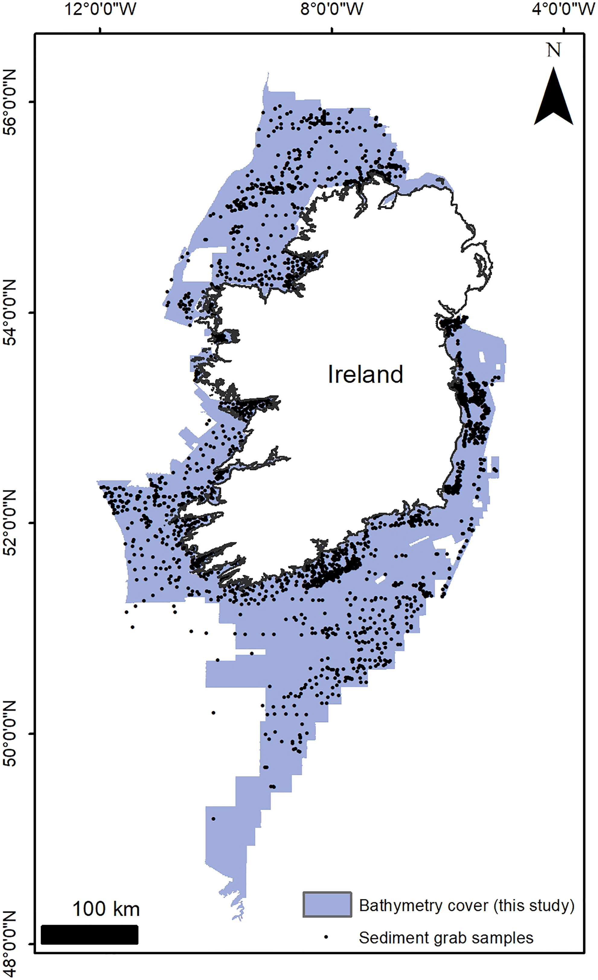
Figure 1 Areal extent of the INFOMAR bathymetric data used in this study, with the location and density of ground-truthing sediment samples consulted at the labelling stage.

TABLE 1

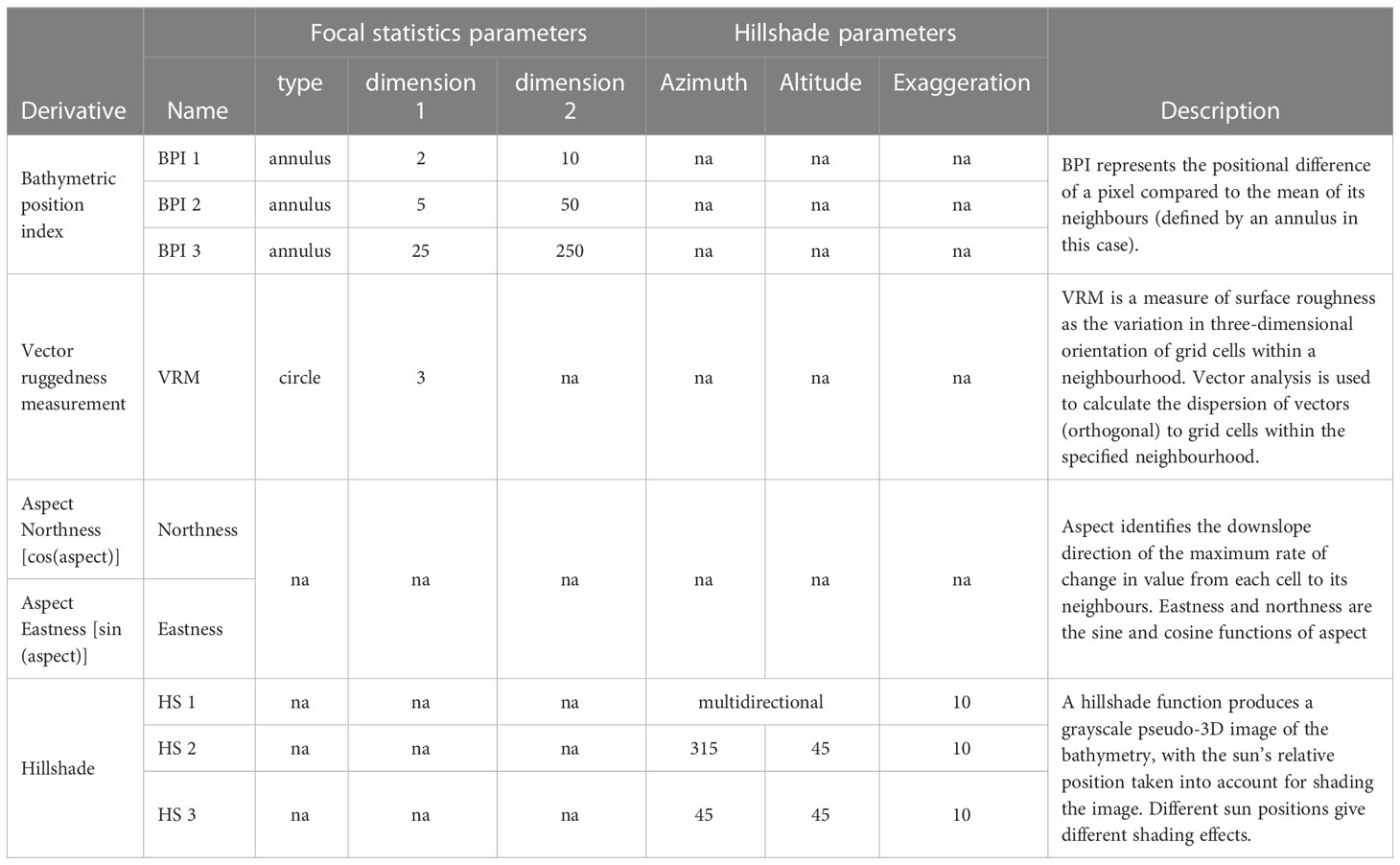
Table 1 List of derivatives and production parameters utilised in this study.

For the purposes of FCNN model training, the bathymetry and derivatives were normalised to a double precision value between 0 and 1 based on the minimum and maximum value recorded or calculated in the case for derivative layers.

2.2 Classification system and labelling

To train the weakly supervised convolutional neural network, we had to define a dataset from which the model could learn the relationship between bathymetry and derivative data and the landforms present. So firstly, a suitable classification system had to be chosen. The classification system adopted is derived from the Mareano-INFOMAR-Maremap-Geoscience Australia (MIM-GA) two-part marine geomorphology scheme, a standardised seabed mapping glossary aimed to enable more consistent seabed classifications (Dove et al., 2016; Dove et al., 2020). This framework independently describes seabed features according to their observed physical structure (Morphology), and the more subjective interpretation of their origin and evolution (Geomorphology). The separation between physical structure and genesis aligned well with the scope of the machine learning-based mapping of this study, where classes were defined based upon the textural characteristics of the surface rather than apparent geological nature or proper geomorphological definitions. This mapping approach was chosen both because of the general lack of geological ground-truthing for novel marine datasets, and for the exploratory nature of the exercise. In general, defined classes describe archetypal seabed textures which, in various combinations, form seabed landforms. The basic distinction between sediment and rock landforms was nonetheless retained (see Table 2), and the INFOMAR sediment grab dataset (https://www.infomar.ie/maps/interactive-maps/seabed-and-sediment) was consulted at the labelling stage (Figure 1). Three principles for classification were adopted (following the advice in Barrett et al., 2022): (a) classes had to be representative of the diversity of seabed morphologies encountered on the Irish continental shelf. This is a “completeness” rule; FCNNs classify pixels in maximum-likelihood fashion, therefore it is essential to fully capture the problem domain as the FCNNs cannot create a new class, or leave a space blank, if an unknown type of seabed is encountered. (b) The classification sets were kept simple and short, as a comprehensive, lengthy list of classes would potentially create difficulties in the training process and especially create more subjective inconsistencies during the labelling work carried out by the expert, and (c) last, but most importantly, classes had to be distinct so that their differences could be confidently isolated visually by the human mapper. This step is critical as the labelling stage may introduce subjectivity and inconsistencies in class delineation that can affect the capabilities of the networks. Therefore, care was taken to semantically define each class, making sure that delineation could be performed with a high level of confidence notwithstanding the limited geological knowledge.

TABLE 2

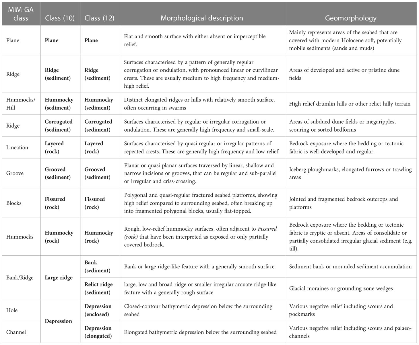
Table 2 Classifications adopted in this study with either 10 or 12 classes and their correspondence to the MIM-GA classification system (Dove et al., 2020).

2.2.1 Terrain and landform classes

A list of 10 classes (Table 2, Figure 2) was considered sufficient to capture the morphological domain of the study area. These classes include three types (or textures) of hard substrate – Fissured, Hummocky and Layered (rock), which comprise bedrock outcrops of meta-/sedimentary and igneous nature but can also include rough or rubbly glacial surfaces which are often hardly distinguishable from bedrock. Corrugated and Ridge (sediment) capture the extensive current-induced bedform fields, respectively the short wavelength megaripples, sediment ribbons or dunes and the larger dunes of different type (transverse, linear, trochoidal etc.) which occur especially in the Irish and Celtic seas (Van Landeghem et al., 2009; Creane et al., 2022). The Irish shelf glacial vestiges, which include prevalently moraines (Ó Cofaigh et al., 2012) and drumlin fields (Benetti et al., 2010) are captured in the Large Ridge and Hummocky (sediment) classes respectively, although we included the Celtic “megaridges” (Lockhart et al., 2018) and sediment banks in the Large Ridge class. The Depression class includes the bathymetric lows on the shelf, which are prevalently channel-like features including scouring, palaeofluvial channels/tunnel valleys (Giglio et al., 2022) and some isolated cases of large pockmarks. Finally, finer scale, elongated depressions or incisions as iceberg ploughmarks and furrowing are represented by the Grooved (sediment) class. The Plane class act as filler for the areas of smooth and featureless terrain. A second list of 12 classes (Table 2, Figure 2) was created to test the performance of the FCNNs with a slightly more complex problem. The second classification set was established increasing the detail for Large Ridge and Depression, splitting them respectively into Bank (sediment) and Relict Ridge (thus dividing the sediment banks from the glacial ridges), and Depression (enclosed) and Depression (elongated) (thus separating circular or quasi circular scouring and pockmarks from channels and elongated scours).

FIGURE 2

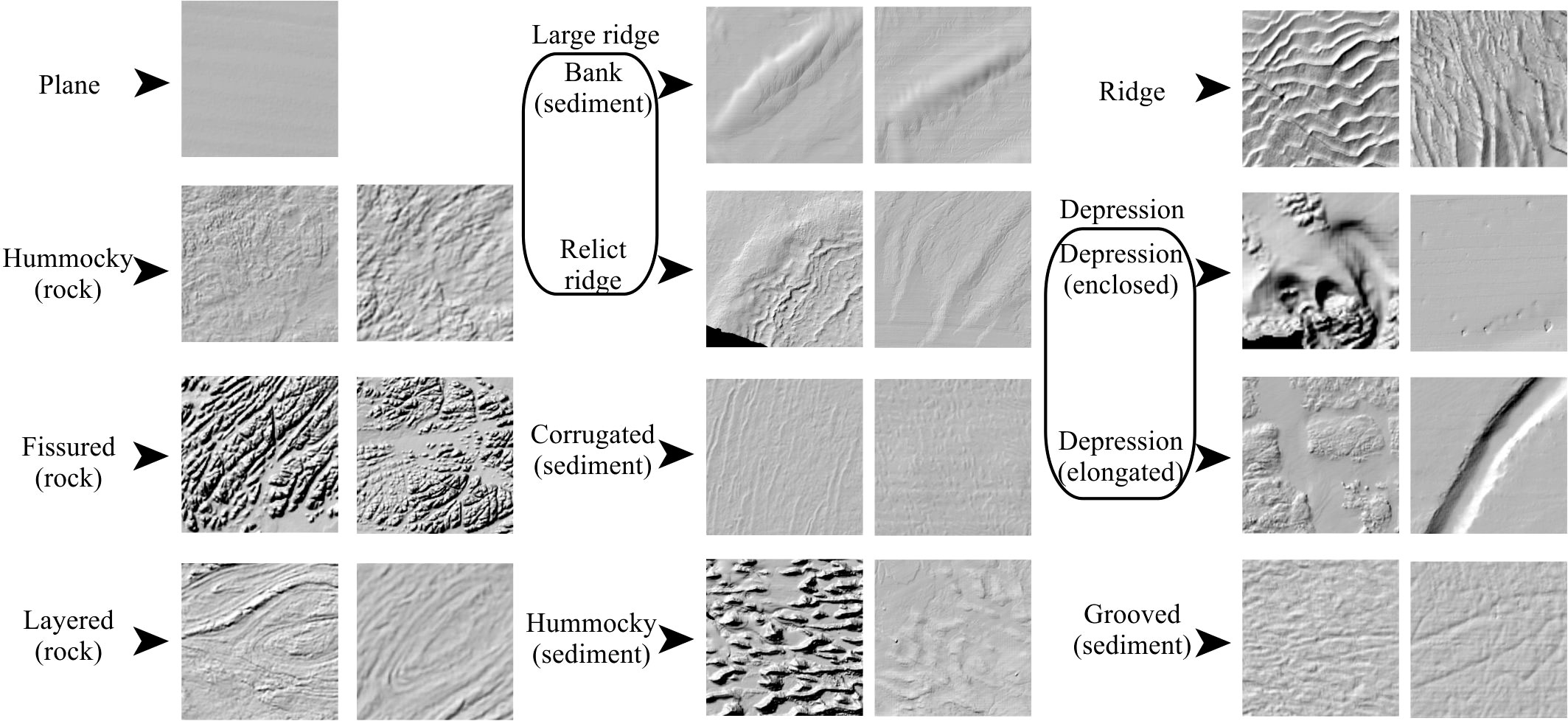
Figure 2 General overview of the textures and geometries of the classes.

2.2.2 Labelling procedures

The labelling of seabed classes was carried out by a single human annotator (the first author) utilising expert judgement with the support of published studies and sediment grain size data for ground-truthing (GT samples in Figure 1) available from the INFOMAR website. Classes were labelled by manually digitising polygons on ArcGIS 10.6 and making sure they contained only the landforms or terrain textures of interest, partially or completely, regardless of their dimensions. Therefore, naturally larger landforms (e.g. the class Large Ridge) are defined by larger labels. Two sets of labels were created, one containing 50 labels per class, and a second with 100 labels per class. The labelled areas constitute only a very small proportion of the total study area (97,526 km²), with the 100-label set covering only 3.2% of the total, the 50 label (12 classes) 2.8% and the 50 labels (10 classes) 2.57%.

Each digitised polygon contains a unique semantic value associated to the landform or terrain texture class. FCNNs were trained with rasterised labels that contain one-to-one mappings of pixels from input layers (Long et al., 2014). The rasterised labels employed to train FCNNs were created using the geographic coordinates stored in each digitised polygon label and converting real-world coordinates for each vertex to image-coordinates. Training pseudo-images were created by centre-cropping 256 x 256 pixel (Figure 3) blocks containing multi-layered raster (bathymetry and derivatives) data. By centre-cropping digitised label polygons, the edges of each pseudo-image may possess a number of unlabelled pixels, which in turn allows for semi-supervised approaches to be leveraged (see Section 2.3). Two factors are behind the specific dimension of the pseudo-images. Firstly, the power of two (256 = 2⁸) grants numerical ease in image resizing (i.e., the blocks are divided/multiplied by 2) with sequential pooling operations and up-sample. Secondly, the image size is appropriate for GPU memory constraints and mini-batch optimisation. For instance, 256x256 may allow 8 images per batch which was found to be optimal for neural network optimisation, whereas an image of 512x512 allows only 1 to 2 images per batch and converges the neural network incorrectly. In the case digitised polygons covered a region that extended past the 256 x 256 area, centre-crops were split into several 256 x 256 blocks. This process generated 553 training images for the 50 label 12-class, 543 training images for the 50 label 10-class and 1134 training images for the 100 label 10-class. For each dataset, the training imagery was randomly subdivided into mutually exclusive training (90%) and validation (10%) sets.

FIGURE 3

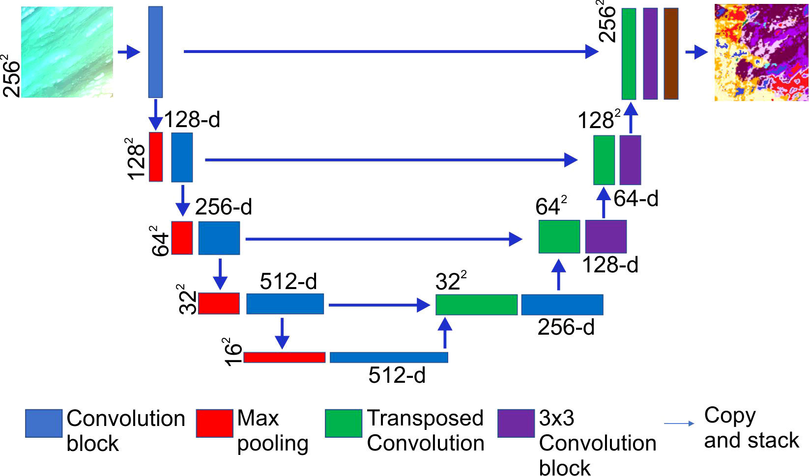
Figure 3 Example of the overall architecture of the FCNN used in this study, showing a VGG13 encoder network. The decoder network applies a transposed 2 by 2 convolution and concatenates feature maps from the encoding network at appropriate resolutions followed by a final 3 by 3 convolution. The final 1 by 1 convolution condenses feature maps to have the same number of channels as the total number of classes in the dataset.

2.3 Fully Convolutional Neural Networks

Fully Convolutional Neural Networks (Long et al., 2014) are an extension of traditional CNN architectures (Krizhevsky et al., 2017) adapted for semantic segmentation. CNNs comprise a series of layers that process lower layer inputs through repeating convolution and pooling operations followed by a final classification layer. Each convolution and pooling layer transform the input image, or in this case bathymetric data, into higher level abstracted representations. FCNNs can be broken down into two networks: an encoder and a decoder network. The encoder network is identical to a CNN, except the final classification layer is removed. The decoder network applies transposed convolutions in order to up-sample feature maps back to the original input size, and each decoding stage combines corresponding feature maps created by the encoder network. The final classification layer utilizes 1 by 1 convolution kernels (Lin et al., 2014) to transform the original bathymetric data and derivatives source into a set of dense probabilities using a softmax transfer function. Network weights and biases are adjusted through gradient descent by minimizing the loss function between network outputs and the ground truth pixel labels.

The overall architecture of the FCNN used in this study (Figure 3) is based on a U-Net (Ronneberger et al., 2015) and the encoder networks are VGG-13 and ResNet50 (Simonyan and Zisserman, 2015; He et al., 2017). Residual learning using ResNet encoders has proven to surpass very deep neural networks such as VGG, but for completeness in results we experimented with both encoder networks. The decoder network applies a transposed 2 by 2 convolution for a learnt up-sample track and concatenates feature maps from the encoding network at appropriate resolutions followed by a final 3 by 3 convolution. The final 1 by 1 convolution condenses feature maps to have the same number of channels as the total number of classes in the dataset (Figure 3).

Semi-supervision is the process of incorporating unlabelled image samples for the optimisation of deep neural networks. This branch of deep learning methods is more applicable when unlabelled data are readily available, while labelled instances are often hard, expensive, and time-consuming to collect. Semi-supervised methods can be capable of building better classifiers that compensate for the lack of labelled training data and therefore present a cost-effective solution to label acquisition. In this study, where semantic segmentation was achieved with a pixel classifier, the masks that were used to label pixels did not cover entire 256x256 pseudo-images and therefore every pseudo-image had pixels that were left unlabelled. This condition allowed for unsupervised loss terms to be added into the optimisation process and thus for semi-supervision to be implemented. The supervised loss term is calculated by processing a mini batch of images $X\in {ℝ}^{B\times C\times H\times W}$ and corresponding segmentation maps $Y\in {ℝ}^{B\times C\times H\times W}$, where B, C, H and W are batch size, number of input channels, height and width. The network produces per-pixel logits $\overline{Y}\in {ℝ}^{B\times K\times H\times W}$- where K is the number of target classes. The softmax transfer function (1) converts network scores into probabilities by normalizing all K scores for each pixel to sum to one:

$$\begin{array}{c}{P}_k(x)=\frac{e^{\overline{Y_k}(x)}}{{\Sigma }_{k^{\prime }=1}^K{e}^{\overline{Y_{k^{\prime }}}(x)}}(1)\end{array}$$

Where, $x\in \text{Ω};\text{Ω}\subseteq {\mathbb{Z}}^2$ is a pixel location and $P_k(x)$ is the probability for the $k^{th}$ channel at pixel location x. The negative log-likelihood loss is calculated between segmentation maps and network probabilities:

$$\begin{array}{c}L=-{\displaystyle \sum _{\text{k}=1}^{\text{K}}{Y}_k(x) \log (P_k(x)) (2)}\end{array}$$

For each image, the supervised loss is the sum of all losses for each pixel using Equation (2) and averaged according to the number of labelled pixels in Y. Full details on the use of semi-supervision can be found in Hobley et al. (2021). The training parameters and convergence of FCNNs was analysed by testing multiple settings for learning rate and batch size, and assessing computed confusion matrices over several consecutive runs of the algorithm. This ensured that a fair range of different convergence approaches was evaluated. Furthermore, for the semi-supervised approach, several different loss weights were experimented to tune for the unsupervised loss term. The best performing networks were trained for 300 epochs with a batch-size of 12 using AdamW optimiser with a learning rate set to 0.001. With regards to the semi-supervised approach, the unsupervised loss was scaled down by a factor of 10 and the confidence threshold for teacher prediction was set to 0.97. All FCNNs were implemented and trained using Pytorch version 10.2, the code is freely available on our GitHub repository: https://github.com/BrandonHobley/geomorph_deep.

2.4 Quality assessment

The quantitative metrics of interest to evaluate a classification algorithm are precision and recall (Equations (3) and (4)). These metrics are adequate to test classification algorithms over different datasets as well as their capability to detect false positives and false negatives. Precision and recall are metrics that can show how a classifier performs for each specific class, where precision measures the ability of the model to identify only the relevant instances, while recall measures the ability to detect correctly the occurrence of a class of interest. For instance, in a dataset with 17 confirmed landforms and 121 false landforms, an algorithm that detects every case as false would have an accuracy of 87%, but at the same time it would have an extremely poor recall of 13%. The F1-score (Equation (5)) is the harmonic mean of recall and precision, giving a suitable generalised single figure of merit to convey the performance of a classifier.

$$\begin{array}{c}precision=\frac{true positive}{true positive+false positive} (3)\end{array}$$

$$\begin{array}{c}recall=\frac{true positive}{true positive+false negative}(4)\end{array}$$

$$\begin{array}{c}F1 score=2 \times \frac{recall \times precision}{recall+precision}(5)\end{array}$$

The quantitative evaluation metrics listed above are valid if the dataset is labelled, which in our study covers a small subset of the total surface mapped. Therefore, these results can give an indication of a particular classifier performance, but visual inspection is still required to fully grasp the capabilities of FCNNs for bathymetric data.

3 Results

3.1 Model performance

For this study, 40 different FCNN model runs were carried out, and total mean of their performances are presented in Table 3. Precision, recall and F1 scores for each class and model are instead given in the Supplementary Material.

TABLE 3

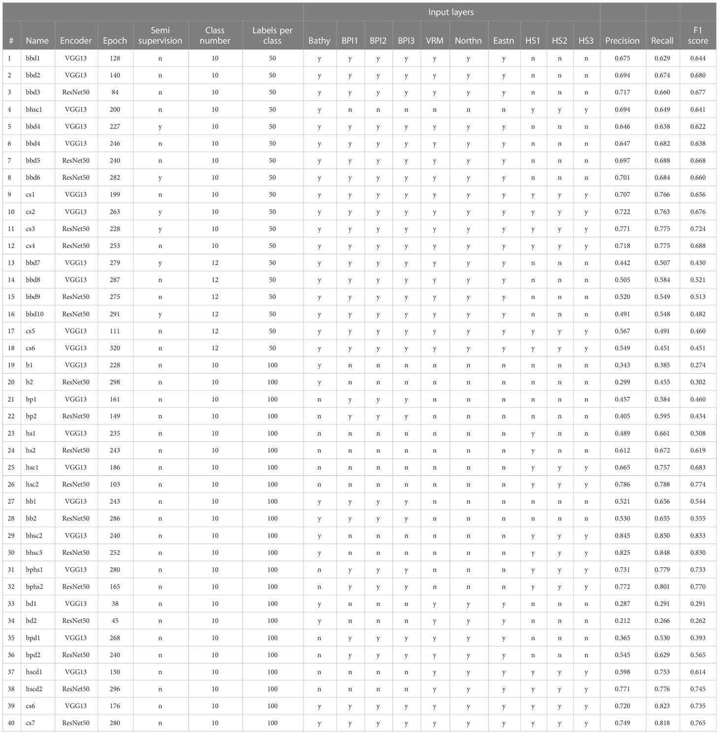
Table 3 Complete list of model results from this study.

The first set of results (models #1 to #12) shows the initial tests carried out on the two different encoders (VGG13 and ResNet50) comparing their efficacy and assessing the utility of semi-supervision and some preliminary combinations of input layers. Overall, the scores show that neither VGG13 nor ResNet50 outperforms the other, although ResNet50 produces slightly better scores at the second decimal point, with increases between 0.01 and 0.05 (e.g. compare models #6 and #7 or #10 and #11).

The use of semi supervision does not improve significantly nor consistently the results, contributing to positive or negative fluctuations. For example, ResNet50 model #11 acquires 0.053 points in Precision compared to non-supervised #12 (Figure 4), with no change in Recall. ResNet50 model #8 gains only 0.004 points in Precision and loses 0.004 points in Recall compared to unsupervised model #7. VGG13 models seem instead to suffer more the application of semi-supervision, leading to higher loss in scores (e.g. compare model outputs #5 and #6).

FIGURE 4

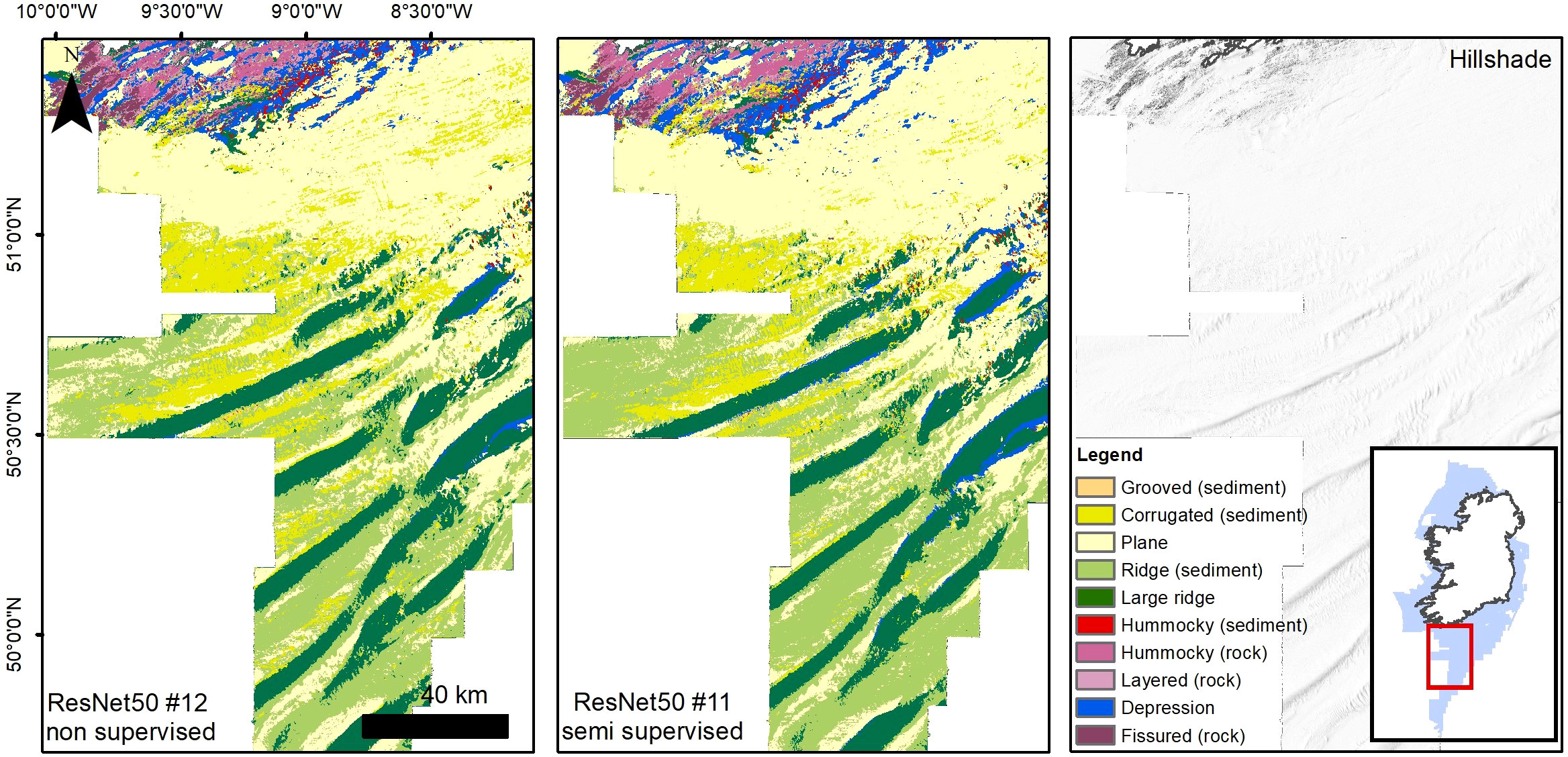
Figure 4 Comparison between non-supervised and supervised ResNet50 model runs #11 and #12. A visual inspection reveals only minor differences in the overall classification.

The best model results were achieved using the complete set of input layers, with ResNet50 models #11 and #12 giving F1 scores of 0.724 and 0.688 respectively. Evaluation metrics are supported by the visual assessment of the resulting thematic maps, where models #11 and #12 show the most visually pleasing results (Figure 4). Nonetheless, high scores were also obtained limiting the input to a combination of bathymetry, BPIs, VRM and Aspect functions (models #3 and #8, with F1 scores of 0.677 and 0.660) or bathymetry and hillshades (model #4, F1 score of 0.641). In order to test the contribution of the input layers to the model predictions, a series of additional model runs were carried out using both encoders but without implementing the semi-supervision -which the previous results reveal to be relatively erratic, and increasing the number of labels to 100 per class, to gauge the effect of boosting label number to model performance.

The results of this series of tests are presented in Table 3, model numbers #19 to #40. As expected, the scores show an overall improvement caused by the increase in the number of labels from 50 to 100. While the time effort required to create labels for the classes is doubled (from 500 to 1000 labels in total), the improvements are significant, up to ~0.19 points, i.e., from 0.641 to 0.833 when comparing the F1 scores of the best VGG13 bathymetry and hillshade results (#4 vs #29).

Once again ResNet50 runs are slightly more successful in evaluation metrics compared to VGG13, with ResNet50 scoring higher in F1 8 times out of 11 model runs.

The exploration of the usefulness of each input layer in model performance provides strong indications that the hillshades are the most valuable set of layers for a correct prediction of morphological classes. Models that utilise hillshades have consistently higher scores than those that do not (cf. for example models #21 with #31 or #33 with #37, Table 3). The use of hillshades alone provides very good results (model #26 F1 score: 0.774), although the combination of layers with different azimuths is essential and a single hillshade is insufficient to produce an accurate map. Overall, the combination of the other derivatives alone or with bathymetry leads to substantially inferior predictions, with Precision scores consistently under 0.59 and Recall scores only slightly better. Aspect functions and VRM do not seem to provide useful information to the models, on the contrary their addition is detrimental to their performance. For example, bathymetry as input layer alone (#19 and #20) contributes to a better score than bathymetry combined with aspect functions and VRM (#33 and #34). While the bathymetric position indexes improve the predictions of the bathymetry baseline, they do not seem to enhance significantly the performance of the hillshade layers, with oscillating results when comparing the “HS full” baselines (models #25 and 26) and the “BPI + all HS” (models #31 and 32). The only layer that does improve the predictions of the hillshades alone is the bathymetry, with model runs #29 and 30 presenting the highest scores obtained in this study (VGG13, Precision 0.845, Recall 0.850). Visually comparing the map outputs of hillshades alone against bathymetry-supported hillshades shows improvement in score metrics obtained by the latter as reflected in the outlook of the map (Figure 5), although the crispness of the boundaries is somewhat diminished, creating more “padded” class interfaces and generalisations.

FIGURE 5

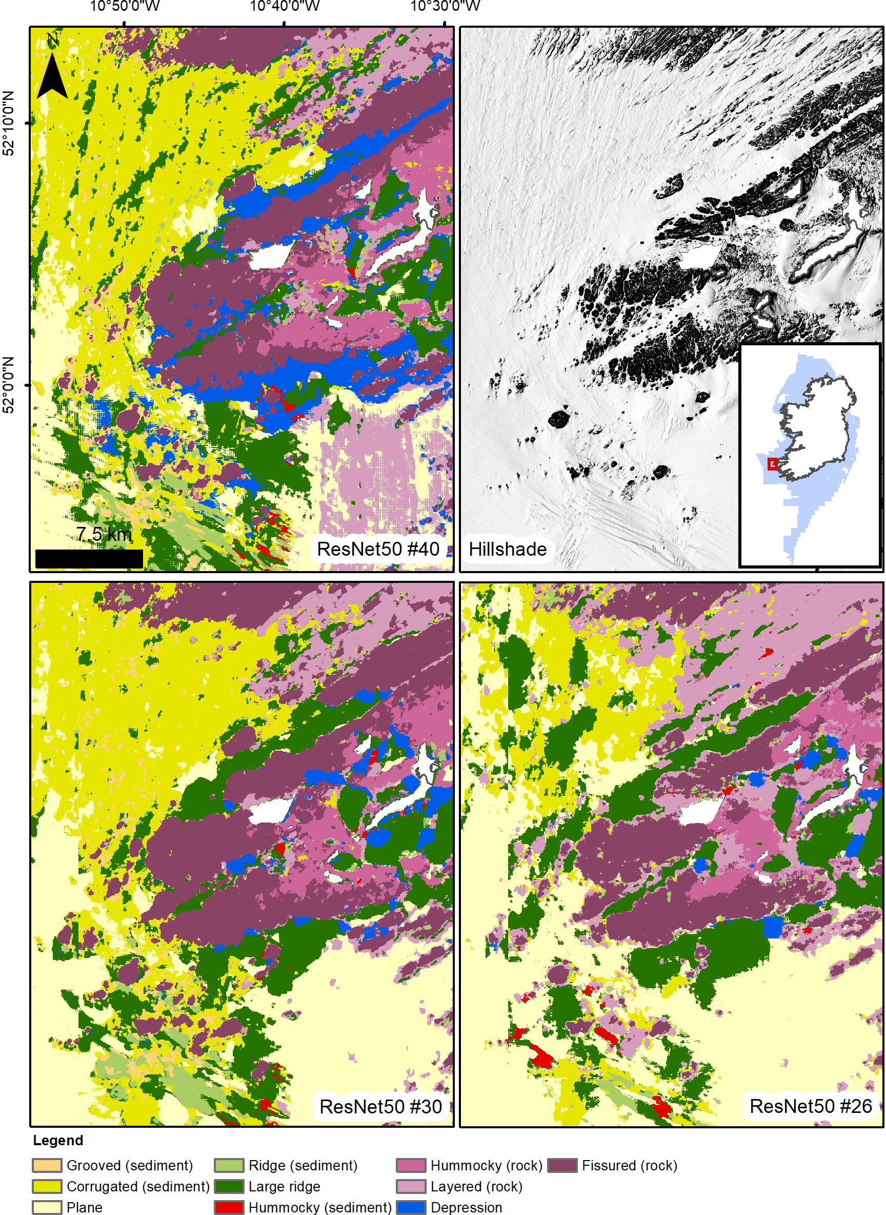
Figure 5 Comparison between the results of ResNet model #40 (complete set of layers), #30 (bathymetry and hillshades) and #26 (only hillshades); visual inspection supports the better accuracy metrics obtained by ResNet50 model #30.

The effect of the combination of all the input layers is given in runs #39 and 40, where the scores are only slightly superior to the model runs of the hillshades, but inferior to the bathymetry and hillshades runs. Overall, Large Ridge, Plane and Fissured (rock) are the three most successfully identified classes by all 10-class models, with an average F1 score of 0.884, 0.772 and 0.716 respectively. Corrugated (sediment), Hummocky (sediment) and Layered (rock) score instead the lowest across all models, with average F1 scores of 0.471, 0.466 and 0.423. The confusion matrices (see the Supplementary Material) show that the prevalent misinterpretation is related to Type II errors (false negatives) where Layered (rock) is classified as Plane, Hummocky (sediment) as Depression and Corrugated (sediment) as Large Ridge. Probable causes for these misinterpretations are treated in the discussion.

Finally, models #13 to #18 (Table 3) show the results of separate tests carried out to investigate the performance of the FCNNs with an increased number of labels. All the results show a substantial decrease in all the scores when moving from the 10 class to the 12 class problem, with Precision and Recall ranging between 0.442-0.567 and 0.451-0.584. Confusion matrices show a decline in accuracy in all classes, and not only those that were split. Depression (enclosed) and Bank (sediment) scored the lowest amongst the classes, showing that the separation from the original and more general Depression and Large Ridge classes (10 class division) weakens the training.

3.2 Modal voting and combined map

The use of several permutations and combinations of different input layers allows for an ensemble learning scenario to be leveraged. We have tested this hypothesis with a simple modal voting of FCNN pixel classifications for the 10 best performing models (both in terms of scores and visual quality), which produced an excellent map with an overall F1 score of 0.96 and class precisions and recalls superior to 0.87. The results and full map are presented in Table S1 and Figure S1 in the Supplementary Material.

4 Discussion

Scores and qualitative assessment of the results have shown that both ResNet50 and VGG13 encoders can achieve good accuracy, with performances driven mostly by the nature of the input layers and the quantity and precision of the labelling. The unsuccessful attempt with 12 classes is most likely caused by a fallacy in the semantic definition of these classes more than weakness of the networks, and it shows that FCNNs can be very susceptible to deceptive labelling. In the first set of tests the best score result was given by ResNet50 model #11, that included all input layers; however, our subsequent analysis of layer contribution shows that the best results are achieved with hillshades and bathymetry only. It must be said that this discrepancy relies on the comparison with a single observation in the first set (i.e. model #4 vs models #9 to 12), and if we take the worst performing model with all input layers (model #9), its scores are not too different from those of hillshade-based model #4 (only Recall being significantly higher in #9). The limitation in sample comparison coupled with the consistent observation that non-hillshade derivatives do not enhance the performance even in the best of cases, support the conclusion that either model #4 is an underperforming outlier or that the doubling of labels has substantially improved the prediction performance based on hillshades. The evaluation metrics improvement generated by the addition of the bathymetry layer to the hillshades input is possibly partly due to the nature of the offshore physiography, where some classes are preferentially found at specific bathymetric ranges. For example, bedrock outcrops are focussed close to the coastline, and unusually high F1 scores for Fissured (rock) and Hummocky (rock) in the bathymetry-based models (#19, #20, see Table S1 in Supplementary Material) strengthen the suspicion of a regional bias. Therefore, the utility of the bathymetry input is potentially lower in different datasets.

Figures 6–8 give an overview of the results provided by the best performing model (#30) and the combined modal vote map. A qualitative assessment of the maps shows that slightly better performances are sometimes achieved to the detriment, in places, of boundary crispness and detail. The evaluation metrics, calculated on a pixel basis, give a good approximation of the effectiveness of a model, however in order to fully assess the models’ performance and potential for seabed mapping studies, we need to consider the results in term of boundary position, nature of misclassifications, type of class misclassified and general distribution of errors.

FIGURE 6

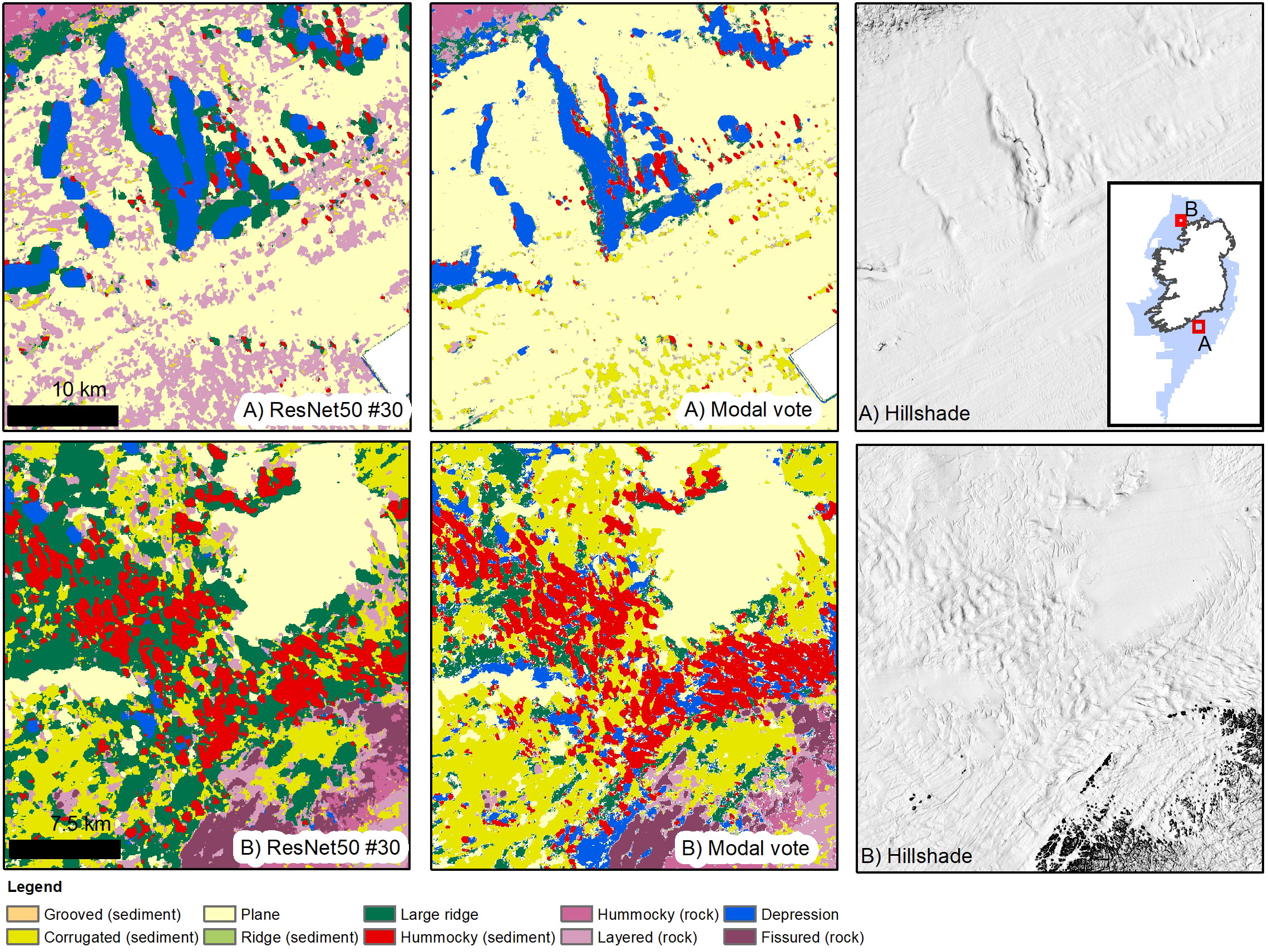
Figure 6 Results from best performing ResNet50 model (#30 – bathymetry and hillshades only) and the modal vote map. While producing overall the best precision and recall scores amongst the model runs, model #30 has underperformed in the detection of the Layered (rock) class (F1 score 0.584), completely misinterpreting the sorted bedforms in the Celtic Sea as rock (A). The modal vote map is instead effective in recognising the bedforms, having better efficacy in identifying Layered (rock) (F1 score 0.90). The glacial streamlined terrain in (B) is well captured by model #30, with only minor mixing between Large Ridge and Hummocky (sediment) where Rogen moraines become larger and are intertwined with larger underlying morainic ridges. While the modal vote map gives also a fair depiction of the area, it overestimates the presence of Depressions, probably due to the interference of the BPI layers.

FIGURE 7

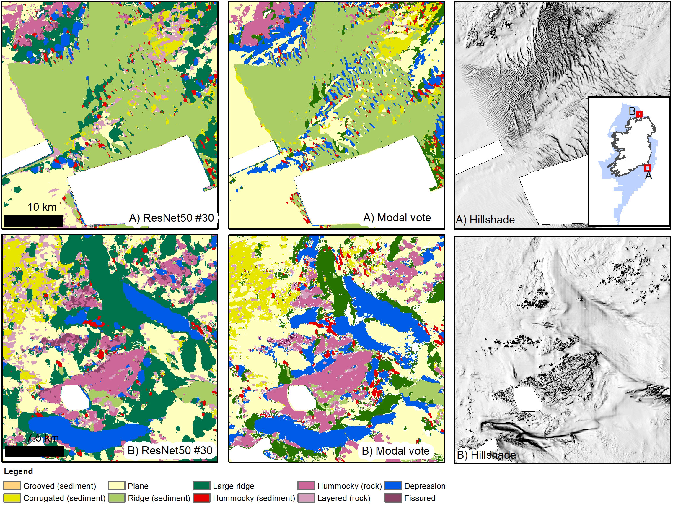
Figure 7 Results from best performing ResNet50 model (#30 – bathymetry and hillshades only) and the modal vote map. (A) Model #30 classifies correctly the extent of the large dune field, although once again the Layered (rock) class is erroneously predicted in liminal places. Both (A) and (B) show well the higher detail provided by the modal vote map, for example in (A) singular dune ridges are mapped correctly at the centre of the field, while for model #30 they are generalised with the surrounding flat or depressed terrain.

FIGURE 8

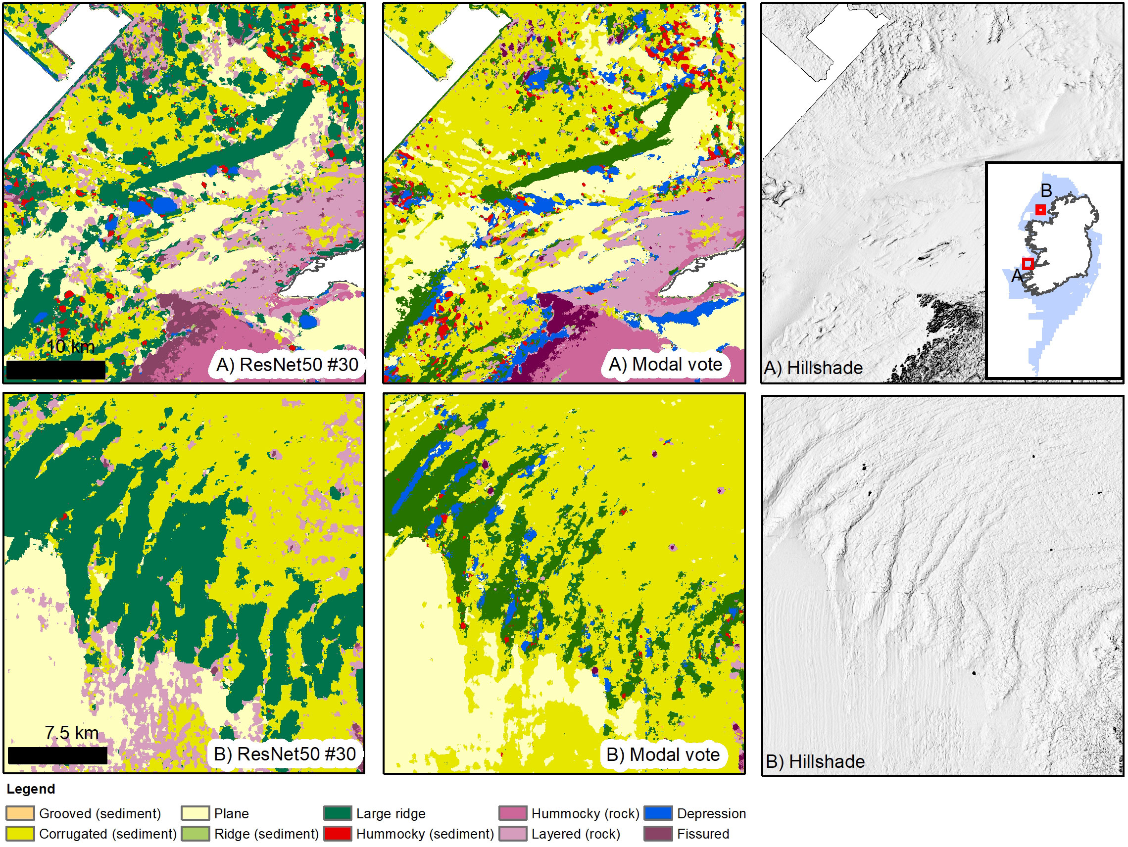
Figure 8 Results from best performing ResNet50 model (#30 – bathymetry and hillshades only) and the modal vote map. (A) this inset shows the overinterpreted Depressions for the modal vote map adjacent to the rocky outcrops, possibly caused by the BPI layers and totally absent for model #30. (B) model #30 correctly identifies the series of moraines in Donegal Bay, while the modal vote map produces a result which is a mixture of textural interpretation (corrugated seabed over the moraines) and larger features interpretation. The bathymetry artefacts that cover the otherwise featureless seabed in the southern portion of the inset have caused misinterpretations in both models; in particular model #30 shows again the confusion in predicting the location of Layered (rock), assigning the artefacts that value.

4.1 Sources of error and uncertainty

In the breakdown of evaluation metrics for each class (Table S1 in Supplementary Material) the three most recurring weakest predictions are linked to the classes Corrugated (sediment), Hummocky (sediment) and Layered (rock). Coupling the observations of class type misinterpretation (see Results) and the qualitative assessment of the map outputs has led to the identification of three main types of errors or uncertainty.

Misclassifications linked to liminal spaces between classes is the first type of ambiguities we discuss (Figures 9A, B). This misclassification is reflected in the significant confusion between Layered (rock) and Plane or Hummocky (sediment) and Depression. Stratified, gently dipping bedrock possesses significant extents of planar features within them (bedding planes), that transition into fine elongated and often isolated ridges. This texture is sometimes misidentified as Plane, but in unlabelled data can also be observed as Layered (rock) in areas of sorted bedforms, that possess similar geometry. A similar case is provided by the Hummocky (sediment) class, which includes the occurrences of drumlins (oval shaped, glacial-flow aligned, moraine hills formed beneath fast-moving ablating ice flows). The drumlins are surrounded by depressed areas, the “connecting surface” between the high relief landforms. Models tended to confuse the proximal interconnecting surface as Depression instead of “drumlin”, leading to the lower score. In defence of the networks, it is often very difficult even for a geomorphologist to find the “correct” place to draw a boundary to define a landform (Smith and Mark, 2003). One major reason that labelling was carried out by a single expert, was to try to achieve maximum consistency in delineation, as another geomorphologist might introduce subjective bias and training conflicts for the networks. Moreover, complex terrains or where class assignment felt ambiguous were deliberately not labelled, leaving effectively the model to decide. We have stressed in the Methods section that good care was taken in the definition of distinctive semantic classes, however these errors indicate that morphological textures form part of a spectrum that is fundamentally difficult to compartmentalise (e.g., at what scale and configuration does a corrugation become a hummock or vice-versa)?, and the shortcomings of the FCNNs are at least partly by-products of natural variability and the inability of a set of classes to fully capture it. Without using a more complex set of classes and fuzzy classifiers it is not possible to treat any existing terrain variation.

FIGURE 9

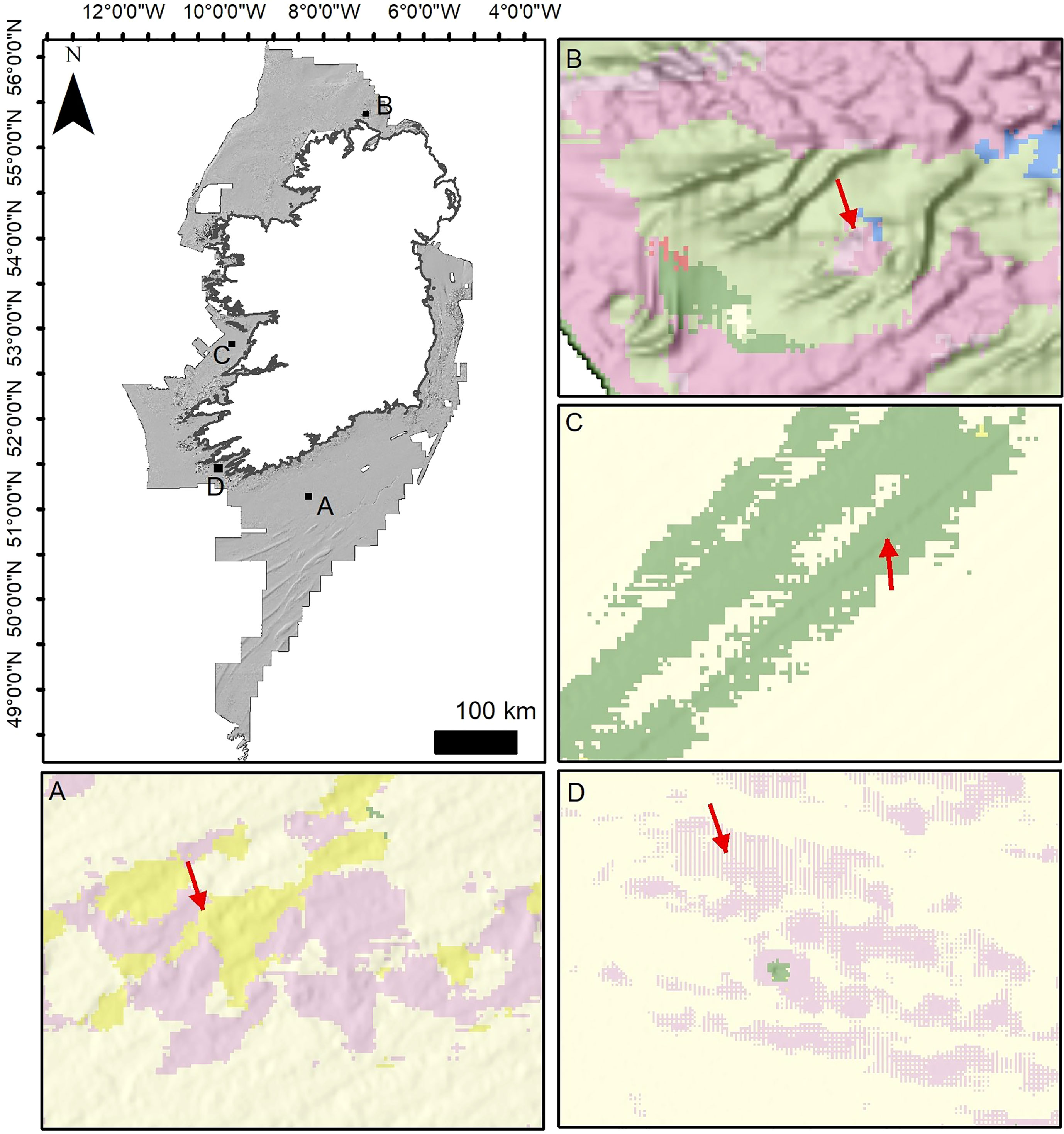
Figure 9 Types of error and ambiguities encountered in the maps. (A, B) sharp class transitions/interfaces and misclassification due to the ambiguous nature of the terrain. This is especially evident in (B), where the dunes cross a rugged bedrock terrain with a similar signature. (C) bathymetry artefacts caused by MBES swath merging and correction that leads to a striping effect (misclassified as Large Ridge). (D) bathymetry artefacts and pixelation produced by low quality older MBES data.

The second type of ambiguity is related to scale (Figures 7, 8, 10). Our classifications included the class Large Ridge (or Bank (sediment) and Relict ridge), which can be significantly bigger than other terrain or landform classes. This factor of scale ambiguity was introduced wittingly into the models, as we wanted to explore the “style” and ability of the networks to disentangle the problem of multiscale classification, which is very common in geomorphology and habitat mapping. If restricted to create a single map layer with a small number of classes, the human mind would prioritise the assignation of a class depending on what they think is the most important attribute to classify. So, for example, a large moraine which is covered by a boulder field might be preferentially mapped as “moraine”, even though both classes identify a correct characteristic of the ground. The hierarchical nature of BTM (Walbridge et al., 2018; Goes et al., 2019; de Oliveira et al., 2020) perpetuates this problem. In our results, this multiscale ambiguity is well reflected in the misclassification of Corrugated (sediment) as Large Ridge; corrugated surfaces such as smaller dunes or sorted bedforms occur extensively on the shelf and can overprint larger features, such as sediment banks or large moraines. The networks preferentially choosing the classification as Large Ridge might reduce the scores in the evaluation metrics but do not technically produce a wrong interpretation, rather a partial one. In some instances (e.g. the on shelf edge, see Figure 10), model predictions have dissected longer wavelength dunes (i.e. large underlying landforms) interpreting them partially as Large Ridges and partially as Corrugated (sediment), where the superficial sorted bedforms are more pronounced. Class prioritisation seems to be dependent on the way the model has learned the classes and boundaries, which in turn depends on adjusted weights and biases the model has learned during model training. However, understanding the individual activations and the internal workings of the neural network would require a study of class activation maps or the visualisation of deconvolutional layers (Noh et al., 2015).

FIGURE 10

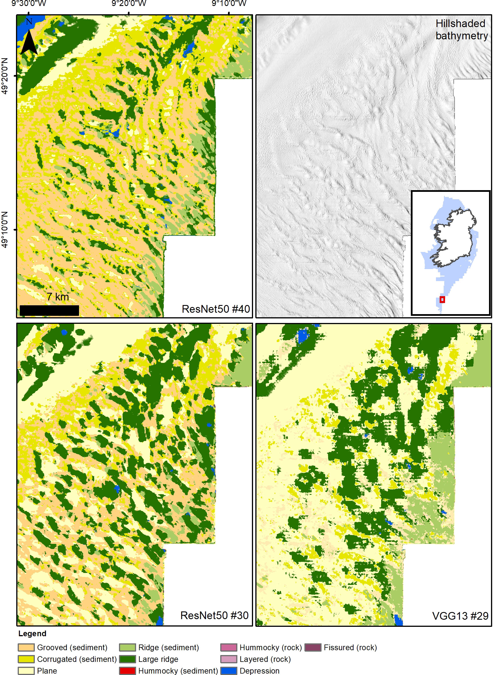
Figure 10 Representation of the different classification styles adopted by the networks when dealing with “nested” bedforms with different dimensions (large dunes, finer megaripples and sorted bedforms) using discrete and non-overlapping classes. All models map the most visible class in an area, reaching different competing results. Models #30 and #40 produce good alternative representations, while model #29 fails to reach a proper depiction of the area.

Finally, a third type of recurring errors is connected to an inherent problem of the input layers: namely artefacts. MBES data can present many type of artefacts mostly caused by the limits of the instrument, the motions of the survey vessel (dynamic systematic errors), poor tidal or water sound velocity control causing vertical shifts and sound refraction. These artefacts are difficult to eliminate completely and a common obstacle in automated marine mapping (Lecours et al., 2017). Artefacts are recurrent in the extensive INFOMAR MBES bathymetry dataset, which is a combination of data from hundreds of different surveys with an array of vessels and survey operators, acquired with different (improving) instrumentation, in the space of about 25 years. The topographic variability introduced may consist in pixelation (salt-and-pepper effects), undulation along the swath, striping effects and cliff-like edges, and the vertical difference is often comparable with real features at seabed (e.g. megaripples or furrowing) (Figures 9C, D). Additionally, our hillshades are particularly susceptible to this kind of “topographic noise”, as they are vertically exaggerated to enhance the visibility of faint terrain patterns, which diminishes considerably their effectiveness. While a study of the effect of artefacts was outside the scope of this paper, it is reasonable to affirm that much stronger predictions can be achieved with a “cleaner” dataset.

4.2 Habitat mapping applications

Morphological maps provide the backbone for seabed habitat mapping studies, with classifications commonly obtained using semi-automated techniques as OBIA, BTM or other GIS tools (Harris et al., 2014; Goes et al., 2019; Linklater et al., 2019; Arosio et al., 2021) that segment the seabed in discrete parcels subsequently classified on the basis of pixel group statistics or geometrical characteristics. While grounded on mathematical rules and granting replicability, these techniques lack flexibility (e.g. how to treat morphological exceptions or near-isomorphisms) and require a good measure of engineering. Moreover, rules applied in one seabed region do not necessarily work elsewhere, so each dataset might need to be treated differently. On the contrary, FCNNs can provide the flexibility needed to capture any instance of discrete landforms or terrain textures without requiring ad hoc segmentation protocols (OBIA) or formulation of classification rulesets (BTM).

A semi-quantitative assessment of the effectiveness of the FCNN predictions for habitat mapping can be made comparing bedrock or sediment texture substrates to existing maps. We compared the predicted FCNN “bedrock” classes (Fissured, Layered and Hummocky (rock)), with the bedrock substrate layer produced by INFOMAR and available on the INFOMAR portal (INFOMAR, 2022). In Figure 11 we take the models with best scores in “bedrock” prediction (model #29 and the modal vote map) and overlap the INFOMAR layer. We limit the comparison area to a subsection of the entire dataset (indicated in Figure 11C), as parts of the INFOMAR layer are mapped at very low resolution (e.g. the areas in Figure 11C pointed by the red arrows), introducing further deviations, and in other zones the Hummocky (rock) class includes also rough glacial till substrate. The best comparison is provided by the modal vote map, with a total bedrock area of 2721 km² (INFOMAR = 2336 km²) and an overlap of 77%. Model #29 has a slightly better overlap (~78%), but has also a larger area mapped as rock (3276 km²). Most of this excess bedrock is caused by misinterpretation of Layered (rock) (Figure 11D), which is over-represented in the model (F1 score 0.58). These numbers have to be taken with a pinch of salt, the mapping approaches are different (e.g. in the INFOMAR dataset the fissures in the bedrock outcrops are given another class), at a slightly different resolution and using different input layers (the INFOMAR map relies abundantly on backscatter data). Nonetheless, there is a broad agreement between the two, and the FCNNs consistently predict bedrock where it has been effectively mapped (see Figure 11). Moreover they give further information on the texture of the bedrock, which can be useful for habitat predictions (Novaczek et al., 2017). A similar comparison can be made with submarine dune fields. In Figure 12 we compare the general location of submarine dune ridges extracted using semi-automated techniques and checked manually (Arosio et al., 2023) with the class Ridge (sediment) in the best performing models (#12 and the modal vote map). Once more the results show an overall agreement, with Ridge (sediment) predictions corresponding with dune field areas (Figures 12A, B). In some places the FCNN is more efficient in identifying subtler ridges (e.g. Figure 12F), however in parts the related classes Large Ridge and Corrugation (sediment) were preferentially selected (e.g. Figures 12E, F). The models show higher levels of confusion in the presence of trochoidal dunes (Figure 12D) that are often misclassified as Fissured (rock) indicating that the labelling is not effective enough to train for this particular morphological distinction.

FIGURE 11

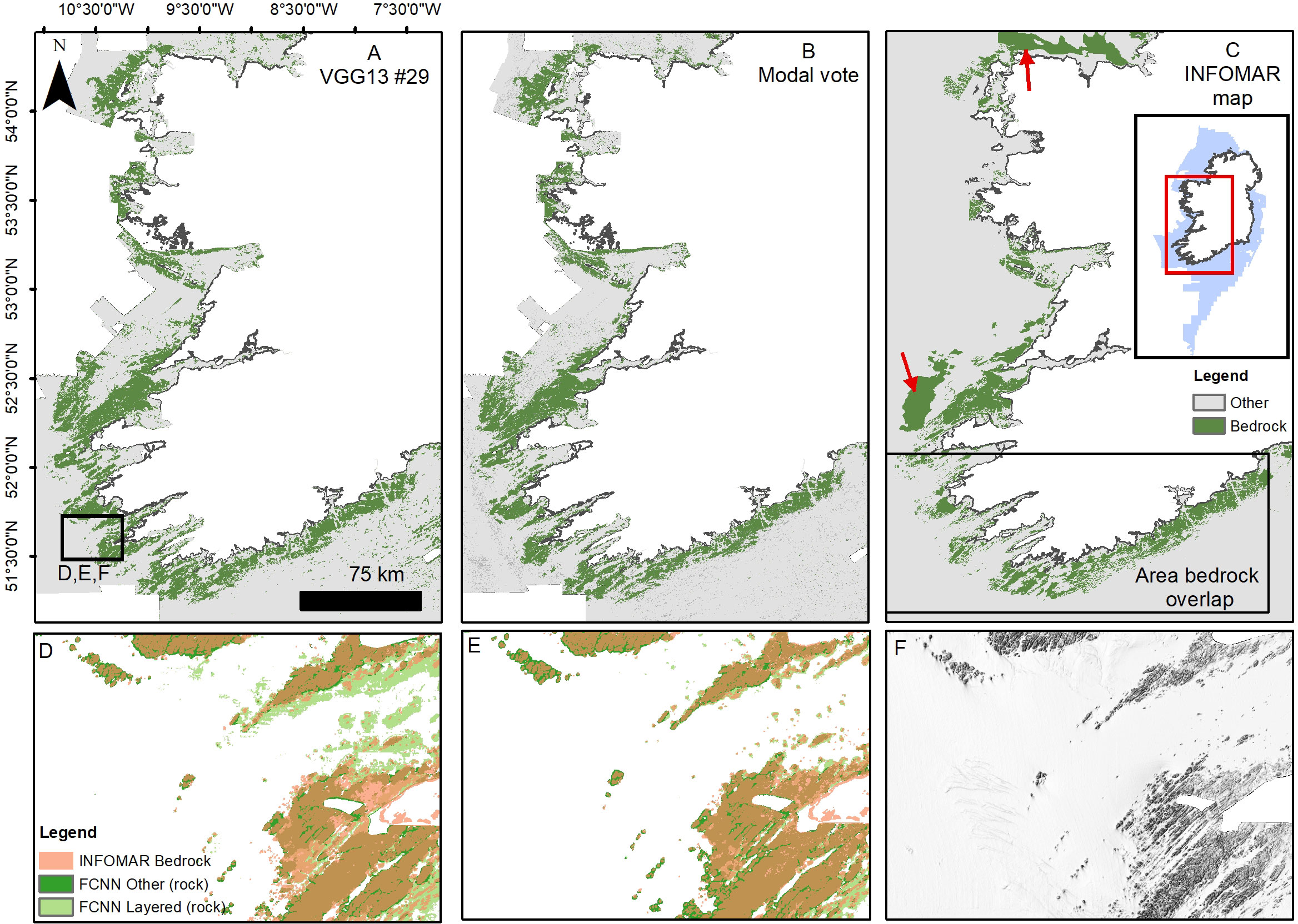
Figure 11 Bedrock mapping results for the best achieving models (in rock-related classes) and comparison with INFOMAR substrate map (A–C). Insets (D, E) show a zoom-in for the results of models #29 and the modal vote map respectively, and the amount of correspondence to the INFOMAR shapefile. The INFOMAR bedrock vector shapefile (in light red) is overlaid on the FCNN green shapefile. Inset (F) shows the hillshaded bathymetry of the same area.

FIGURE 12

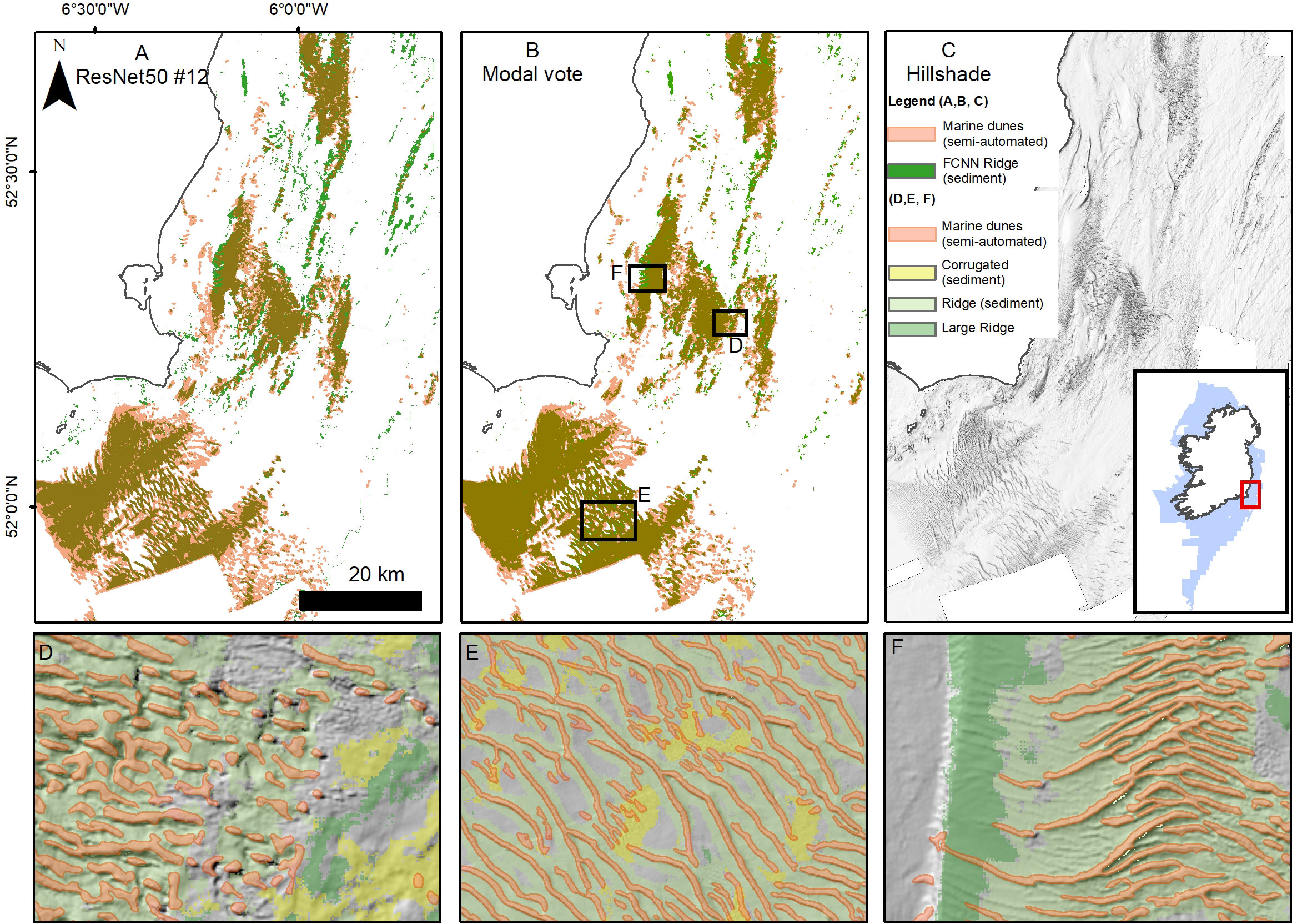
Figure 12 Submarine dune fields (Ridge, sediment) mapping results for the best achieving models and comparison with unpublished semi-automated mapping performed by the authors (A–C). The semi-automated dune vector shapefile (in light red) is overlaid on the FCNN green shapefile. Insets (D–F) show zoom-ins of the modal vote map.

4.3 Final considerations

This exploratory study has shown that FCNNs have considerable potential for the creation of large scale seabed landforms and terrain textures map, and that even with relatively modest human input the results can be satisfactory. A clear semantic class definition and label delineation (including numerous boundary cases) will improve the accuracy of the classification, while a more rigorous consistency in mapping scale will most likely reduce ambiguity. Our results show that the optimisation of derivative selection helps the model outputs, and a combination of hillshaded layers contribute substantially to prediction improvements. Further insights on the contribution of each layer could be obtained using techniques based on feature importance, as saliency maps (e.g. Simonyan et al., 2014). The ensemble voting map, which constituted the best outcome of these experiments, clearly shows the utility of using learnt biases on different subsets of input data, and that assembling predictions from several ‘weak’ learners outperforms a single ‘expert’ network, which is the premise of ensemble learning (Ganaie et al., 2022). For further work, several FCNNs could be trained concurrently on different subsets of input data, and a loss could be calculated based on the confidence of individual networks (Goyal et al., 2020; Zhou et al., 2021). The latter is akin to several Decision trees in a Random Forest in classical machine learning (Cutler et al., 2012).

From a habitat mapper’s perspective, the use of FCNNs can be successfully applied to seabed maps for morphological characterisation, and very good results and flexibility can be achieved provided the model is well trained and furnished with clean data. Very large scale mapping endeavours, as that presented in Harris et al. (2014), could be easily replicated and improved upon using FCNNs. Moreover previously trained models could be applied on the new datasets that are being collected and gathered for Seabed 2030. If a sufficient volume of labelled classes is cooperatively assembled in a “dictionary” and made publicly available, it could be used by the community to predict morphological classes across different datasets, improving upon map objectivity and inter-comparison. The time invested in creating such a dictionary would be considerable but worthwhile, as the FCNN method will be eventually better, quicker and easily repeatable compared to semi-automated or manual digitisations. We shared our labelled dataset on GitHub (https://github.com/BrandonHobley/geomorph_deep) as a starting point. While discrete computer power it is necessary, the code is open source and requires a relatively basic level of coding expertise to be run, allowing for a widespread adoption.

FCNNs have also their significant drawbacks. Firstly, they are essentially a blackbox whose internal workings are not fully understood. Secondly, labelling and training at one determinate pixel resolution is most likely not transferable to a different one. So having mapped at 25m/pixel our dataset is probably ineffective to map at 2m/pixel, and more ad hoc labelling will be required. Finally, at this stage of sophistication, FCNNs fail to recognize complex geomorphological processes, especially in cases of isomorphism, so human intervention is still required. This limitation is also caused by the input types themselves, as bathymetry-derived raster data alone are often insufficient (for human geomorphologists too!) to unequivocally identify seabed landforms. Only when different types of datasets (seismic lines, ground-truthing etc.) can be included in the predictions, will machine learning be useful for more complex seabed geological interpretations.

Data availability statement

The raw data supporting the conclusions of this article will be made available by the authors, without undue reservation.

Author contributions

RA conceived the original idea, performed the labelling and analysed the results. BH wrote the neural networks and run the models. RA and BH developed the approach and wrote the manuscript. AL and AW obtained the funding and reviewed the manuscript. FS, LC, and TF reviewed the manuscript. All authors provided useful feedback and helped shape the research. All authors contributed to the article and approved the submitted version.

Funding

RA received funding from the Irish Marine Institute’s research grant PDOC 19/08/03. LC and TF were funded by the European Union’s Horizon 2020 research and innovation programme under Grant Agreement No 862428 (MISSION ATLANTIC).

Acknowledgments

Firstly, we would like to thank the hard work of the captains and crews of the Irish research vessels that assisted in the collection of the INFOMAR dataset. The map contains Irish Public Sector Data (Marine Institute & Geological Survey Ireland) licensed under a Creative Commons Attribution 4.0 International (CC BY 4.0) licence.

Conflict of interest

The authors declare that the research was conducted in the absence of any commercial or financial relationships that could be construed as a potential conflict of interest.

Publisher’s note

All claims expressed in this article are solely those of the authors and do not necessarily represent those of their affiliated organizations, or those of the publisher, the editors and the reviewers. Any product that may be evaluated in this article, or claim that may be made by its manufacturer, is not guaranteed or endorsed by the publisher.

Supplementary material

The Supplementary Material for this article can be found online at: https://www.frontiersin.org/articles/10.3389/fmars.2023.1228867/full#supplementary-material

References

Arosio R., Mitchell P., Hawes J., Bolam S., Benson L., Sperry J. (2021). Small island developing states (SIDS) and the sea: creating high resolution habitat maps to support effective marine management in St. Lucia (Vienna: Presented at the EGU). doi: 10.5194/egusphere-egu21-102

CrossRef Full Text | Google Scholar

Arosio R., Wheeler A. J., Sacchetti F., Guinan J., Conti L. A., Furey T., et al. (2023). The NOMANS_TIF map: ireland’s first complete shallow seabed geomorphology map (Saint-Gilles-Les-Bains: Presented at the GeoHab 2023, La Réunion). doi: 10.5281/zenodo.7890332

CrossRef Full Text | Google Scholar

Barrett A. M., Balme M. R., Woods M., Karachalios S., Petrocelli D., Joudrier L., et al. (2022). NOAH-h, a deep-learning, terrain classification system for Mars: results for the ExoMars rover candidate landing sites. Icarus 371, 114701. doi: 10.1016/j.icarus.2021.114701

CrossRef Full Text | Google Scholar

Benetti S., Dunlop P., Cofaigh C.Ó. (2010). Glacial and glacially-related features on the continental margin of northwest Ireland mapped from marine geophysical data. J. Maps 6, 14–29. doi: 10.4113/jom.2010.1092

CrossRef Full Text | Google Scholar

Blaschke T., Hay G. J., Kelly M., Lang S., Hofmann P., Addink E., et al. (2014). Geographic object-based image analysis – towards a new paradigm. ISPRS J. Photogrammetry Remote Sens. 87, 180–191. doi: 10.1016/j.isprsjprs.2013.09.014

CrossRef Full Text | Google Scholar

Brown C. J., Smith S. J., Lawton P., Anderson J. T. (2011). Benthic habitat mapping: a review of progress towards improved understanding of the spatial ecology of the seafloor using acoustic techniques. Estuarine Coast. Shelf Sci. 92, 502–520. doi: 10.1016/j.ecss.2011.02.007

CrossRef Full Text | Google Scholar

Buscombe D., Wernette P., Fitzpatrick S., Favela J., Goldstein E. B., Enwright N. M. (2023). A 1.2 billion pixel human-labeled dataset for data-driven classification of coastal environments. Sci. Data 10, 46. doi: 10.1038/s41597-023-01929-2

PubMed Abstract | CrossRef Full Text | Google Scholar

Conti L. A., Lim A., Wheeler A. J. (2019). High resolution mapping of a cold water coral mound. Sci. Rep. 9, 1016. doi: 10.1038/s41598-018-37725-x

PubMed Abstract | CrossRef Full Text | Google Scholar

Creane S., Coughlan M., O’Shea M., Murphy J. (2022). Development and dynamics of sediment waves in a complex morphological and tidal dominant system: southern Irish Sea. Geosciences 12, 431. doi: 10.3390/geosciences12120431

CrossRef Full Text | Google Scholar

Cutler A., Cutler D. R., Stevens J. R. (2012). “Random forests,” in Ensemble machine learning. Eds. Zhang C., Ma Y. (New York, NY: Springer New York), 157–175. doi: 10.1007/978-1-4419-9326-7_5

CrossRef Full Text | Google Scholar

de Oliveira N., Bastos A. C., da Silva Quaresma V., Vieira F. V. (2020). The use of benthic terrain modeler (BTM) in the characterization of continental shelf habitats. Geo-Mar Lett. 40, 1087–1097. doi: 10.1007/s00367-020-00642-y

CrossRef Full Text | Google Scholar

de Oliveira L. M. C., Lim A., Conti L. A., Wheeler A. J. (2021). 3D classification of cold-water coral reefs: a comparison of classification techniques for 3D reconstructions of cold-water coral reefs and seabed. Front. Mar. Sci. 8. doi: 10.3389/fmars.2021.640713

CrossRef Full Text | Google Scholar

Diesing M., Green S. L., Stephens D., Lark R. M., Stewart H. A., Dove D. (2014). Mapping seabed sediments: comparison of manual, geostatistical, object-based image analysis and machine learning approaches. Continental Shelf Res. 84, 107–119. doi: 10.1016/j.csr.2014.05.004

CrossRef Full Text | Google Scholar

Diesing M., Thorsnes T. (2018). Mapping of cold-water coral carbonate mounds based on geomorphometric features: an object-based approach. Geosciences 8, 34. doi: 10.3390/geosciences8020034

CrossRef Full Text | Google Scholar

Dove D., Bradwell T., Carter G., Cotteril C., Gafeira J., Green S., et al. (2016). Seabed geomorphology: a two-part classification system (Marine geosciences programme open report no. OR/16/001) (Edinburgh: British Geological Survey).

Google Scholar

Dove D., Nanson R., Bjarnadóttir L. R., Guinan J., Gafeira J., Post A., et al. (2020). A two-part seabed geomorphology classification scheme (v.2); part 1: morphology features glossary (Zenodo). doi: 10.5281/ZENODO.4075248

CrossRef Full Text | Google Scholar

Foroutan M., Zimbelman J. R. (2017). Semi-automatic mapping of linear-trending bedforms using ‘Self-organizing maps’ algorithm. Geomorphology 293, 156–166. doi: 10.1016/j.geomorph.2017.05.016

CrossRef Full Text | Google Scholar

Ganaie M. A., Hu M., Malik A. K., Tanveer M., Suganthan P. N. (2022). Ensemble deep learning: a review. Eng. Appl. Artif. Intell. 115, 105151. doi: 10.1016/j.engappai.2022.105151

CrossRef Full Text | Google Scholar

Gazis I. Z., Schoening T., Alevizos E., Greinert J. (2018). Quantitative mapping and predictive modeling of Mn nodules’ distribution from hydroacoustic and optical AUV data linked by random forests machine learning. Biogeosciences 15, 7347–7377. doi: 10.5194/bg-15-7347-2018

CrossRef Full Text | Google Scholar

Giglio C., Benetti S., Sacchetti F., Lockhart E., Hughes Clarke J., Plets R., et al. (2022). A Late Pleistocene channelized subglacial meltwater system on the Atlantic continental shelf south of Ireland. Boreas, 51, 118–135. doi: 10.1111/bor.12536

CrossRef Full Text | Google Scholar

Goes E. R., Brown C. J., Araújo T. C. (2019). Geomorphological classification of the benthic structures on a tropical continental shelf. Front. Mar. Sci. 6. doi: 10.3389/fmars.2019.00047

CrossRef Full Text | Google Scholar

Goyal M., Oakley A., Bansal P., Dancey D., Yap M. H. (2020). Skin lesion segmentation in dermoscopic images with ensemble deep learning methods. IEEE Access 8, 4171–4181. doi: 10.1109/ACCESS.2019.2960504

CrossRef Full Text | Google Scholar

Harris P. T., Baker E. (2020). Seafloor geomorphology as benthic habitat (Elsevier). doi: 10.1016/C2017-0-02139-0

CrossRef Full Text | Google Scholar

Harris P. T., Macmillan-Lawler M., Rupp J., Baker E. K. (2014). Geomorphology of the oceans. Mar. Geology 352, 4–24. doi: 10.1016/j.margeo.2014.01.011

CrossRef Full Text | Google Scholar

He K., Gkioxari G., Dollar P., Girshick R. (2017). “Mask R-CNN,” 2017 IEEE International Conference on Computer Vision (ICCV). (Venice, Italy) 2980–2988. doi: 10.1109/ICCV.2017.322

CrossRef Full Text | Google Scholar

Hobley B., Arosio R., French G., Bremner J., Dolphin T., Mackiewicz M. (2021). Semi-supervised segmentation for coastal monitoring seagrass using RPA imagery. Remote Sens. 13, 1741. doi: 10.3390/rs13091741

CrossRef Full Text | Google Scholar

Ierodiaconou D., Schimel A. C. G., Kennedy D., Monk J., Gaylard G., Young M., et al. (2018). Combining pixel and object based image analysis of ultra-high resolution multibeam bathymetry and backscatter for habitat mapping in shallow marine waters. Mar. Geophys Res. 39, 271–288. doi: 10.1007/s11001-017-9338-z

CrossRef Full Text | Google Scholar

INFOMAR (2022). Seabed sediment classification Irish waters WGS84 shapefile.

Google Scholar

Ismail K., Huvenne V. A. I., Masson D. G. (2015). Objective automated classification technique for marine landscape mapping in submarine canyons. Mar. Geology 362, 17–32. doi: 10.1016/j.margeo.2015.01.006

CrossRef Full Text | Google Scholar

Juliani C. (2019). Automated discrimination of fault scarps along an Arctic mid-ocean ridge using neural networks. Comput. Geosciences 124, 27–36. doi: 10.1016/j.cageo.2018.12.010

CrossRef Full Text | Google Scholar

Keohane I., White S. (2022). Chimney identification tool for automated detection of hydrothermal chimneys from high-resolution bathymetry using machine learning. Geosciences 12, 176. doi: 10.3390/geosciences12040176

CrossRef Full Text | Google Scholar

Krizhevsky A., Sutskever I., Hinton G. E. (2017). ImageNet classification with deep convolutional neural networks. Commun. ACM 60, 84–90. doi: 10.1145/3065386

CrossRef Full Text | Google Scholar

Lecours V., Devillers R., Edinger E. N., Brown C. J., Lucieer V. L. (2017). Influence of artefacts in marine digital terrain models on habitat maps and species distribution models: a multiscale assessment. Remote Sens. Ecol. Conserv. 3, 232–246. doi: 10.1002/rse2.49

CrossRef Full Text | Google Scholar

Lecours V., Dolan M. F. J., Micallef A., Lucieer V. L. (2016). A review of marine geomorphometry, the quantitative study of the seafloor. Hydrol. Earth Syst. Sci. 20, 3207–3244. doi: 10.5194/hess-20-3207-2016

CrossRef Full Text | Google Scholar

LeCun Y., Bengio Y., Hinton G. (2015). Deep learning. Nature 521, 436–444. doi: 10.1038/nature14539

PubMed Abstract | CrossRef Full Text | Google Scholar

Leitão P. J., Schwieder M., Pötzschner F., Pinto J. R. R., Teixeira A. M. C., Pedroni F., et al. (2018). From sample to pixel: multi-scale remote sensing data for upscaling aboveground carbon data in heterogeneous landscapes. Ecosphere 9, e02298. doi: 10.1002/ecs2.2298

CrossRef Full Text | Google Scholar

Lin M., Chen Q., Yan S. (2014). Network in network. International Conference on Learning Representations (ICLR) (Banff). Available at: http://arxiv.org/abs/1312.4400.

Google Scholar

Linklater M., Ingleton T. C., Kinsela M. A., Morris B. D., Allen K. M., Sutherland M. D., et al. (2019). Techniques for classifying seabed morphology and composition on a subtropical-temperate continental shelf. Geosciences 9, 141. doi: 10.3390/geosciences9030141

CrossRef Full Text | Google Scholar

Lockhart E. A., Scourse J. D., Praeg D., Van Landeghem K. J. J., Mellett C., Saher M., et al. (2018). A stratigraphic investigation of the celtic Sea megaridges based on seismic and core data from the Irish-UK sectors. Quaternary Sci. Rev. 198, 156–170. doi: 10.1016/j.quascirev.2018.08.029

CrossRef Full Text | Google Scholar

Long J., Shelhamer E., Darrell T. (2014). Fully convolutional networks for semantic segmentation (Boston, MA, USA: IEEE Conference on Computer Vision and Pattern Recognition (CVPR)), 3431–3440. doi: 10.1109/CVPR.2015.7298965

CrossRef Full Text | Google Scholar

Lundine M. A., Brothers L. L., Trembanis A. C. (2023). Deep learning for pockmark detection: implications for quantitative seafloor characterization. Geomorphology 421, 108524. doi: 10.1016/j.geomorph.2022.108524

CrossRef Full Text | Google Scholar

Ma Z., Mei G. (2021). Deep learning for geological hazards analysis: data, models, applications, and opportunities. Earth-Science Rev. 223, 103858. doi: 10.1016/j.earscirev.2021.103858

CrossRef Full Text | Google Scholar

McClinton T. J., White S. M., Sinton J. M. (2012). Neuro-fuzzy classification of submarine lava flow morphology. Photogrammetric Eng. Remote Sens. 78, 605–616. doi: 10.14358/PERS.78.6.605

CrossRef Full Text | Google Scholar

Micallef A., Le Bas T. P., Huvenne V. A. I., Blondel P., Hühnerbach V., Deidun A. (2012). A multi-method approach for benthic habitat mapping of shallow coastal areas with high-resolution multibeam data. Continental Shelf Res. 39–40, 14–26. doi: 10.1016/j.csr.2012.03.008

CrossRef Full Text | Google Scholar

Noh H., Hong S., Han B. (2015). Learning deconvolution network for semantic segmentation (Santiago, Chile: IEEE International Conference on Computer Vision (ICCV)), 1520–1528. doi: 10.1109/ICCV.2015.178

CrossRef Full Text | Google Scholar

Novaczek E., Devillers R., Edinger E., Mello L. (2017). High-resolution seafloor mapping to describe coastal denning habitat of a Canadian species at risk: Atlantic wolffish (Anarhichas lupus). Can. J. Fish. Aquat. Sci. 74, 2073–2084. doi: 10.1139/cjfas-2016-0414

CrossRef Full Text | Google Scholar

Ó Cofaigh C., Dunlop P., Benetti S. (2012). Marine geophysical evidence for late pleistocene ice sheet extent and recession off northwest Ireland. Quaternary Sci. Rev. 44, 147–159. doi: 10.1016/j.quascirev.2010.02.005

CrossRef Full Text | Google Scholar

Palafox L. F., Hamilton C. W., Scheidt S. P., Alvarez A. M. (2017). Automated detection of geological landforms on Mars using convolutional neural networks. Comput. Geosciences 101, 48–56. doi: 10.1016/j.cageo.2016.12.015

CrossRef Full Text | Google Scholar

Ronneberger O., Fischer P., Brox T. (2015). “U-Net: convolutional networks for biomedical image segmentation,” in Medical image computing and computer-assisted intervention – MICCAI 2015, lecture notes in computer science. Eds. Navab N., Hornegger J., Wells W. M., Frangi A. F. (Springer International Publishing, Cham), 234–241. doi: 10.1007/978-3-319-24574-4_28

CrossRef Full Text | Google Scholar

Rubanenko L., Perez-Lopez S., Schull J., Lapotre M. G. A. (2021). Automatic detection and Segmentation of barchan dunes on Mars and earth using a convolutional neural network. IEEE J. Sel. Top. Appl. Earth Observations Remote Sens. 14, 9364–9371. doi: 10.1109/JSTARS.2021.3109900

CrossRef Full Text | Google Scholar

Simonyan K., Vedaldi A., Zisserman A. (2014). Deep inside convolutional networks: visualising image classification models and saliency maps. Workshop at International Conference on Learning Representations. doi: 10.48550/arXiv.1312.6034

CrossRef Full Text | Google Scholar

Simonyan K., Zisserman A. (2015). Very deep convolutional networks for Large-scale image recognition (San Diego: International Conference on Learning Representations (ICLR)). Available at: https://arxiv.org/abs/1409.1556.

Google Scholar

Smith B., Mark D. M. (2003). Do mountains exist? towards an ontology of landforms. Environ. Plann B Plann Des. 30, 411–427. doi: 10.1068/b12821

CrossRef Full Text | Google Scholar

Summers G., Lim A., Wheeler A. J. (2021). A scalable, supervised classification of seabed sediment waves using an object-based image analysis approach. Remote Sens. 13, 2317. doi: 10.3390/rs13122317

CrossRef Full Text | Google Scholar

Tarvainen A., Valpola H. (2017). “Mean teachers are better role models: weight-averaged consistency targets improve semi-supervised deep learning results,” in 31st Conference on Neural Information Processing System. Presented at the NIPS, Long Beach, USA.

Google Scholar

Valentine A. P., Kalnins L. M., Trampert J. (2013). Discovery and analysis of topographic features using learning algorithms: a seamount case study. Geophysical Res. Lett. 40, 3048–3054. doi: 10.1002/grl.50615

CrossRef Full Text | Google Scholar

Van Landeghem K. J. J., Uehara K., Wheeler A. J., Mitchell N. C., Scourse J. D. (2009). Post-glacial sediment dynamics in the Irish Sea and sediment wave morphology: data–model comparisons. Continental Shelf Res. 29, 1723–1736. doi: 10.1016/j.csr.2009.05.014

CrossRef Full Text | Google Scholar

Walbridge S., Slocum N., Pobuda M., Wright D. J. (2018). Unified geomorphological analysis workflows with benthic terrain modeler. Geosciences 8, 94. doi: 10.3390/geosciences8030094

CrossRef Full Text | Google Scholar

Wang Y., Di K., Xin X., Wan W. (2017). Automatic detection of Martian dark slope streaks by machine learning using HiRISE images. ISPRS J. Photogrammetry Remote Sens. 129, 12–20. doi: 10.1016/j.isprsjprs.2017.04.014

CrossRef Full Text | Google Scholar

Wilhelm T., Geis M., Püttschneider J., Sievernich T., Weber T., Wohlfarth K., et al. (2020). DoMars16k: a diverse dataset for weakly supervised geomorphologic analysis on Mars. Remote Sens. 12, 3981. doi: 10.3390/rs12233981

CrossRef Full Text | Google Scholar

Yasir M., Rahman A. U., Gohar M. (2021). Habitat mapping using deep neural networks. Multimedia Syst. 27, 679–690. doi: 10.1007/s00530-020-00695-0

CrossRef Full Text | Google Scholar

Zhou T., Lu H., Yang Z., Qiu S., Huo B., Dong Y. (2021). The ensemble deep learning model for novel COVID-19 on CT images. Appl. Soft Computing 98, 106885. doi: 10.1016/j.asoc.2020.106885

CrossRef Full Text | Google Scholar