 Victoria Marja Sofia Ollus1,2*‡
 Martin Biuw3
 Andrew Lowther4‡
 Per Fauchald2‡
 John Elling Deehr Johannessen4‡
 Lucía Martina Martín López5Kalliopi C. Gkikopoulou6†‡W. Chris Oosthuizen7‡
 Ulf Lindstrøm1,3
- 1UiT The Arctic University of Norway, Department of Arctic and Marine Biology, Tromsø, Norway
- 2Department of Arctic Ecology, Norwegian Institute for Nature Research, Tromsø, Norway
- 3Norwegian Institute of Marine Research, Marine Mammal Research Group, Norwegian Institute of Marine Research, Tromsø, Norway
- 4Norwegian Polar Institute, Research Department, Norwegian Polar Institute, Tromsø, Norway
- 5Asociación Ipar Perspective, Sopela, Spain
- 6Sea Mammal Research Unit, Scottish Ocean Institute, University of St Andrews, St Andrews, United Kingdom
- 7Center for Statistics in Ecology, Environment and Conservation, Department of Statistical Sciences, University of Cape Town, Cape Town, South Africa
Introduction: The Scotia Sea and Antarctic Peninsula are warming rapidly and changes in species distribution are expected. In predicting habitat shifts and considering appropriate management strategies for marine predators, a community-level understanding of how these predators are distributed is desirable. Acquiring such data, particularly in remote areas, is often problematic given the cost associated with the operation of research vessels. Here we use cruise vessels as sampling platforms to explore seabird distribution relative to habitat characteristics.
Methods: Data on seabird at-sea distribution were collected using strip-transect counts throughout the Antarctic Peninsula and Scotia Sea in the austral summer of 2019-2020. Constrained correspondence analysis (CCA) and generalized additive models (GAM) were used to relate seabird community composition, density, and species richness to environmental covariates.
Results: Species assemblages differed between oceanographic areas, with sea surface temperature and distance to coast being the most important predictors of seabird distribution. Our results further revealed a geographic separation of distinct communities rather than hotspot regions in the study area in summer.
Discussion: These findings highlight the importance of large-scale environmental characteristics in shaping seabird community structure, presumably through underlying prey distribution and interspecific interactions. The present study contributes to the knowledge of seabird distribution and habitat use as well as the baseline for assessing the response of Antarctic seabird communities to climate warming. We argue that cruise vessels, when combined with structured research surveys, can provide a cost-effective additional tool for the monitoring of community and ecosystem level changes.
1 Introduction
Marine ecosystems are under pressure from climate change and increasing human activities, causing habitat degradation, biodiversity loss and consequent changes in species distributions and food webs (Myers & Worm, 2003; Scheffer et al., 2005; Hoegh-Guldberg & Bruno, 2010; Bindoff et al., 2019). In the Southern Ocean, pressures include warming, sea ice reduction, acidification, and commercial fisheries (Barbraud et al., 2012; Chown & Brooks, 2019; Meredith et al., 2019; Bestley et al., 2020). A warming climate is predicted to cause physical and biogeochemical changes in the Southern Ocean, affecting prey distribution and biomass, with knock-on effects on predator distribution (Meredith et al., 2019; Hindell et al., 2020). Temperature-related effects on seabird distribution have already been detected in the southern Indian Ocean (Péron et al., 2010) while ecosystem changes are also predicted to intensify in the Scotia Sea and the Antarctic Peninsula (Meredith et al., 2019). Considering this, a necessary precursor to appropriate marine stewardship is to understand factors affecting the spatial distribution of marine predators such as seabirds (González-Solís & Shaffer, 2009).
The association between seabird communities and biophysical characteristics of the marine environment has been studied extensively (Pocklington, 1979; Abrams, 1985; Hunt et al., 1990; Amorim et al., 2009) and the heterogeneity of environmental features is known to be reflected in species distribution (Nelson, 1980; Hunt et al., 1999; Fauchald et al., 2011b). Seabird communities typically associate with specific habitats, reflecting species’ life history traits and adaptations, and the distribution of their prey (Griffiths et al., 1982; Wahl et al., 1989; Ainley et al., 1994; Fauchald et al., 2000). On a meso-scale (>100 km), upwelling at continental edges and oceanic fronts creates nutrient rich areas where prey, and therefore predators, tend to concentrate (Nelson, 1980; Bost et al., 2009; Bestley et al., 2020).
The Scotia Sea (SS) in the Southern Ocean is an important area for seabirds, showing high diversity and abundance (Shirihai, 2007; Hindell et al., 2020). Due to their differing geographical location and climate, the ocean areas around the northern Antarctic Peninsula (AP), South Georgia and Falkland Islands host different seabird communities. In summer, these are important feeding habitats for both local breeders, and other species migrating from afar, such as Arctic terns (Sterna paradisaea; Egevang et al., 2010; McKnight et al., 2013). Hence the summer seabird assemblages in the SS and AP consist of both visitors and year-round residents, some of which are nonbreeders, spending their time foraging at sea, while others are breeders and consequently central-place foragers, spatially constrained by their nesting sites (Gaston, 2004) and with elevated energetic demands (Markones et al., 2010). There is inter- and intraspecific variation in foraging range among both breeders and nonbreeders (Phillips et al., 2017).
On a meso-scale, the strongest predictors of all seabird distribution patterns tend to relate to prey distribution (Ballance, 2007). In the short-chained food web of the SS and the AP, Antarctic krill (Euphausia superba; hereafter krill) is a keystone species at the mid-trophic level (McCormack et al., 2021) though other crustaceans, fish and cephalopods are also important prey for several seabird species, such as albatrosses and terns (Griffiths, 1982; Barrera-Oro, 2002; Alvito et al., 2015; Moreno et al., 2016). Large swarms of krill attract a variety of seabirds (Shirihai, 2007; Bost et al., 2009; Joiris & Dochy, 2013), as well as fish that in turn serve as food for seabirds looking for larger prey (Barrera-Oro, 2002). Fish and cephalopods are the dominant prey groups for seabirds in northern SS and lower latitude Southern Ocean in general (Griffiths et al., 1982; Xavier et al., 2003; Shirihai, 2007; Cherel et al., 2010). Krill is abundant in the AP and southern SS area (CCAMLR, 2019; Krafft et al., 2019; Perry et al., 2019), where its fishery focuses (Nicol et al., 2012) and coincides with important areas for krill dependent predators (Hinke et al., 2017; Hindell et al., 2020). A growing krill fishery has the potential of posing an indirect threat to seabird populations in the area by enhancing intra and inter-species competition (Trites et al., 2006; Bertrand et al., 2012; Bestley et al., 2020, but see also Ratcliffe et al., 2015). Competition for food resources is assumed to further increase as populations of great whales recover from earlier exploitation, consuming a growing share of the krill stock (Reilly et al., 2004; Tulloch et al., 2019; Zerbini et al., 2019; Baines et al., 2021), though interactions with whales may also have positive effects on seabirds (Enticott, 1986; Veit & Harrison, 2017). Thus, with the additional pressures from rapid climate change (Meredith & King, 2005; Kawaguchi et al., 2013; Meredith et al., 2019), and with the changes that have been proposed to already have taken place (Reid & Croxall, 2001; Atkinson et al., 2004; Atkinson et al., 2019, but see also Meredith et al., 2019), the AP and SS are consequently in need of effective ecosystem-based management (Hinke et al., 2017). Despite the considerable attention given to marine top predators, substantial information gaps on their distribution and habitat use remain and need to be filled to better inform management of the area (reviewed by Chown & Brooks, 2019, and Bestley et al., 2020).
At-sea counts of seabirds are ideally conducted along systematic transects that provide coverage across the area of interest (Tasker et al., 1984; Spear et al., 2004; Goyert et al., 2016; Bolduc & Fifield, 2017). The operation of dedicated research vessels is costly however, particularly in remote areas, which limits the spatial and temporal extent and repetition of systematic surveys. To complement such dedicated research surveys, opportunistic observation platforms such as fishing vessels and scientific vessels supplying research stations are often used for data collection (Péron et al., 2010; Jiménez et al., 2011, European Seabirds at Sea, 2022). Cruise vessels also operate on repeated routes throughout specific seasons and may serve as low-cost observation platforms that allow frequent repetition of surveys (Henderson et al., 2023). This is a considerable advantage particularly in areas that are difficult to access and hence sparsely sampled, and in areas of rapid environmental change for which there is an urgent need for monitoring and ecological knowledge to base management decisions on. However, the predetermined routes of opportunistic sampling platforms, including cruise vessels, often go in straight lines between sites of interest and do not allow for a systematic or stratified sampling design. A systematic sampling design, where transects are laid out to cover a pre-defined study area and relevant environmental gradients, requires dedicated research cruises. Cruise vessels nevertheless allow repeated sampling along straight lines making it possible to study large scale community patterns along environmental gradients at relatively low costs. We therefore argue that cruise vessels represent an underused sampling opportunity that has large potential to add to our knowledge of seabird at-sea distribution when combined with data collected on research cruises or with telemetry data.
We conducted at-sea surveys of seabirds from platforms of opportunity (cruise vessels) transiting the SS and AP several times during the 2019-2020 austral summer. Our study sets out to quantify variation in space use and community composition of seabirds and to link these to habitat-describing physical variables. We hypothesize (1) that spatial variability in seabird community composition is explained primarily by biogeography, i.e., species are associated with specific habitat characteristics that reflect the distribution of preferred prey, breeding sites, and environmental conditions suited for the species’ physiological adaptations, and (2) that seabird diversity and abundance correlate with physical features that enhance prey availability on a meso-scale, consequently varying synchronously between latitudes. We also discuss the utility of cruise vessels as observation platforms for capturing spatial variability in seabird at-sea distribution.
2 Methods
2.1 Study area
The Scotia Sea (SS) in the Atlantic sector of the Southern Ocean (Figure 1, inset) is characterized by the eastward flowing Antarctic Circumpolar Current (ACC), and four associated frontal systems (from north to south: the Subantarctic Front, the Polar front, the southern Antarctic Circumpolar Current front (sACCf), and the southern boundary of the Antarctic Circumpolar Current (sbACC); Orsi et al., 1995). The SS and greater Southwest Atlantic region is a particularly productive part of the Southern Ocean (Prézelin et al., 2000; Atkinson et al., 2001; Kahru et al., 2007). Our study area is located between longitudes 35 and 68°W, and latitudes 51 and 66°S. It consists of coastal areas, shelf waters and deep sea, crosses all fronts of the ACC, and stretches over different climate regimes (Figure 1).
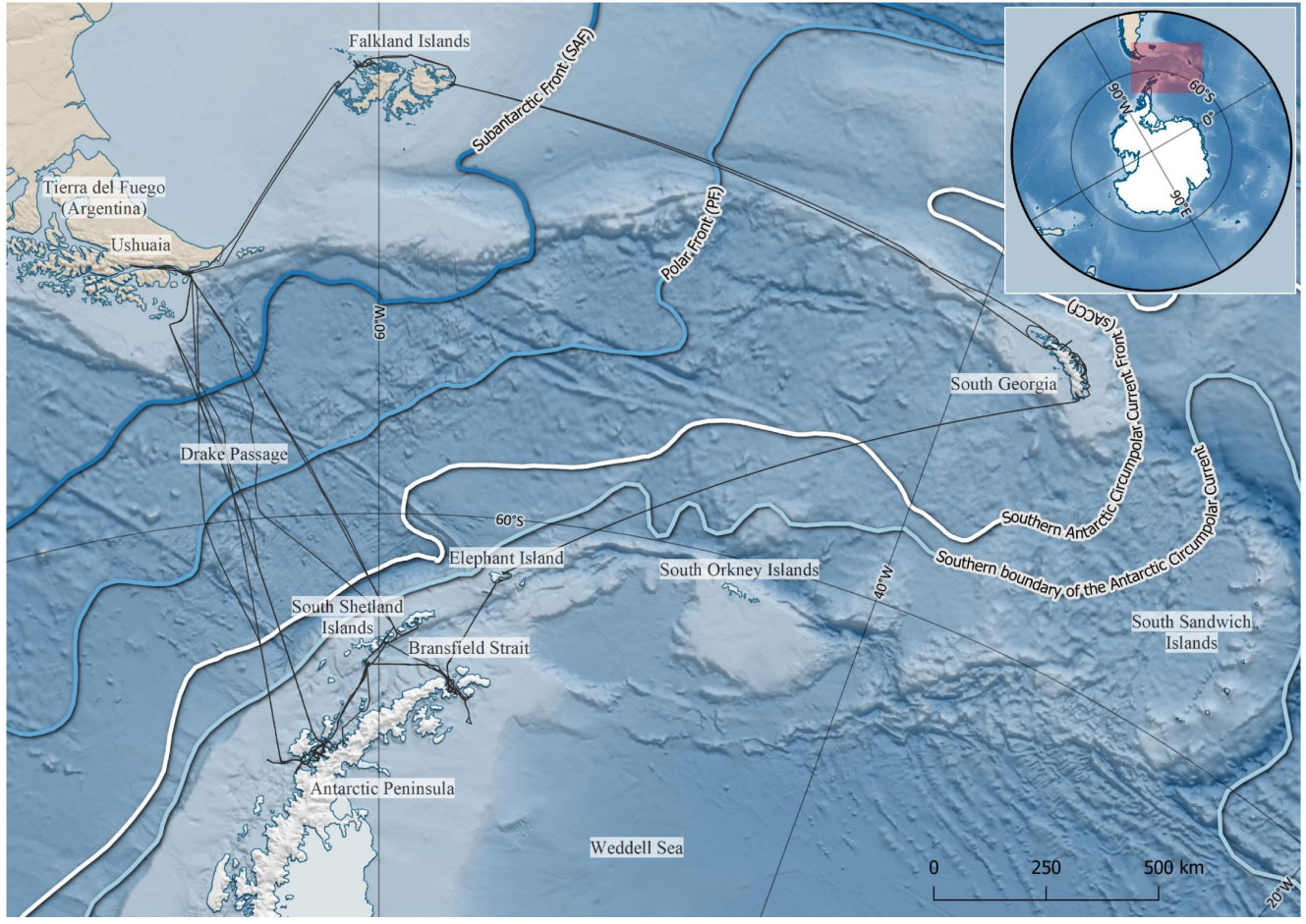
Figure 1 Study area with mean positions of the main oceanographic fronts shown and track lines of the vessels indicated as black lines. Map produced using Quantarctica (Matsuoka et al., 2021) and datasets therein (Orsi et al., 1995; Amante & Eakins, 2009; NOAA National Geophysical Data Center, 2009; Arndt et al., 2013; Liu et al., 2015, SCAR Antarctic Digital Database) in QGIS (QGIS.org, 2019).
2.2 Seabird surveys
At-sea surveys were conducted from two cruise ships (MS Fram and MS Midnatsol, Hurtigruten AS) which ran multiple trips throughout the SS and northern AP during the austral summer of 2019-2020. Observations on MS Midnatsol were made during three consecutive trips from Ushuaia to the AP and back, from 23 November to 28 December 2019. On MS Fram, observations were made during two consecutive trips from Ushuaia, via the Falkland Islands and South Georgia, to the AP and back to Ushuaia, from 10 December 2019 to 19 January 2020. The vessels’ track lines are presented in Figure 1.
Surveys were conducted using a continuous strip-transect count methodology (Tasker et al., 1984). On each ship, a team of two to three observers took turns identifying and counting seabirds from the bridge, approximately 15 m above sea surface. Strip-transect counts were made along transects of 300 m width (distance was estimated by eye after joint training at sea), in time intervals of 10 minutes sampling once every hour, when the ship was in transit and under satisfying weather conditions (visibility > 300 m). A strip width of 300 m has previously been identified as optimal for bird counts at sea when visibility is good (Ballance, 2007; Bolduc & Fifield, 2017). The strip-transect extended from the bow in a 90° arc to the side with better visibility (least glare), either the starboard (0° - 90°) or to the port side (270° - 360°). Observations of seabirds were done by eye, and binoculars were used for species identification when needed.
Some species-specific biases in seabird counts were expected due to size differences, species-specific behavior and methodology. The most obvious potential bias is related to inflated counts of ship-attracted species and multiple counting of individuals that follow the ship (Spear et al., 1992; Hyrenbach, 2001). Further, flying birds moving faster than the vessel or perpendicular to the strip-transect are more likely to enter the strip-transect than swimming birds or birds resting on the sea surface. This leads to flux of birds inside the strip-transect and a positive bias in flying birds in absolute density estimations, if not accounted for with methods described by Tasker et al. (1984); Spear et al. (1992), or van Franeker (1994). Typically, the snap-shot method is used, where the observer conducts instantaneous counts of all flying birds present in the observed field (Tasker et al., 1984). In this study we used a continuous counting method, and a positive bias is expected for some species.
The start time (UTC) for each strip-transect count and the observation data on species and respective abundances were recorded using the Logger 2010 software (Gillespie et al., 2010). The position of the vessel was logged continuously (on a temporal resolution of 1 minute) together with time and speed data using a Globalsat USB GPS receiver, so that observation data could be related to geographical position. Not all birds could be reliably identified to the species level, and the taxonomic groups used for data analysis are presented in Supplementary Table S1.
2.3 Environmental predictors of seabird distribution
We relate seabird distribution to habitat-describing environmental variables that reflect meso-scale (>100 km) processes and are generally considered as cues for biological production. These are 1) distance to coast (km), 2) bathymetric slope (degrees of inclination), 3) sea surface temperature (SST, °C) and 4) the SST gradient over space, defining meso-scale oceanographic fronts (detailed hereafter).
2.3.1 Distance to coast
Distance to coast was calculated as the shortest distance (km) from the start point of a strip-transect to the nearest land mass (island or mainland). Distance to coast was calculated using the coordinates for the start points of the strip-transects and the coordinates for the coastline using the function ‘dist2Line’ in package ‘geosphere’ (Hijmans, 2019) and the SCAR Antarctic Digital Database.
2.3.2 Bathymetric slope
A high bathymetric slope indicates potential areas of upwelling. A raster layer for seabed slope was created based on bathymetric data from an elevation raster of 2000 m resolution (ETOPO1; Amante & Eakins, 2009; NOAA National Geophysical Data Center, 2009) using the ‘slope’ function in QGIS (v 3.10.1; QGIS.org, 2019). Values of seabed slope as degrees of inclination to the horizontal were then derived for the starting position of each strip-transect from the created raster.
2.3.3 Sea surface temperature and its gradient across space
Daily SST data were downloaded from the Physical Oceanography Distributed Active Archive Center (UK Met Office, 2012) with values on a 0.054-degree grid (spatial resolution 0.05 degrees Latitude * 0.05 degrees Longitude), from which SST values were extracted for each strip-transect based on date and coordinates. The sea surface temperature gradient was calculated as the spatial change in SST, using the ‘terrain’ function in the package ‘raster’ (Hijmans, 2020). High values of SST gradient are indicative of oceanographic fronts between water masses of different temperatures. Such frontal areas are usually associated with physical processes such as water mixing, eddy formation and upwelling, which are known to stimulate and/or retain high levels of primary production (Hunt et al., 1999; Kahru et al., 2007).
2.4 Statistical analyses
Data were processed and analyzed using QGIS (QGIS.org, 2019) and R (R Core Team, 2020). The ‘LoggeR’ package (Biuw, 2019) was used to import and pre-process data from the Logger Access database to R.
Vessel speed affects the flux of birds in strip-transects and only strip-transects conducted at a speed of 10-17 knots were included in data analyses. In addition, two strip-transects near South Georgia had extreme abundance of prions (>1000 individuals counted) and were excluded from the statistical analyses. Because we were interested in meso-scale patterns that act on a scale of hundreds of km, observation periods (strip-transects) were binned at a scale of 100 km for the analyses of seabird community composition and seabird density and diversity. Data aggregation on a smaller scale would result in noise from sub-mesoscale processes, while aggregation on a larger scale could cover meso-scale patterns (Fauchald et al., 2000). Binning observations every 100 km along the vessel tracks resulted in 140 groups of observations (six strip-transects at the end of vessel transects fell outside 100-km bins and were omitted) (Figure 2). These groups were used as sample units in the statistical analyses. Values of total seabird density and predictor variables were calculated as means of the values in binned observations. Species richness was calculated as the total number of species observed in 100-km bins and is hence affected by the number of strip-transects within each bin.
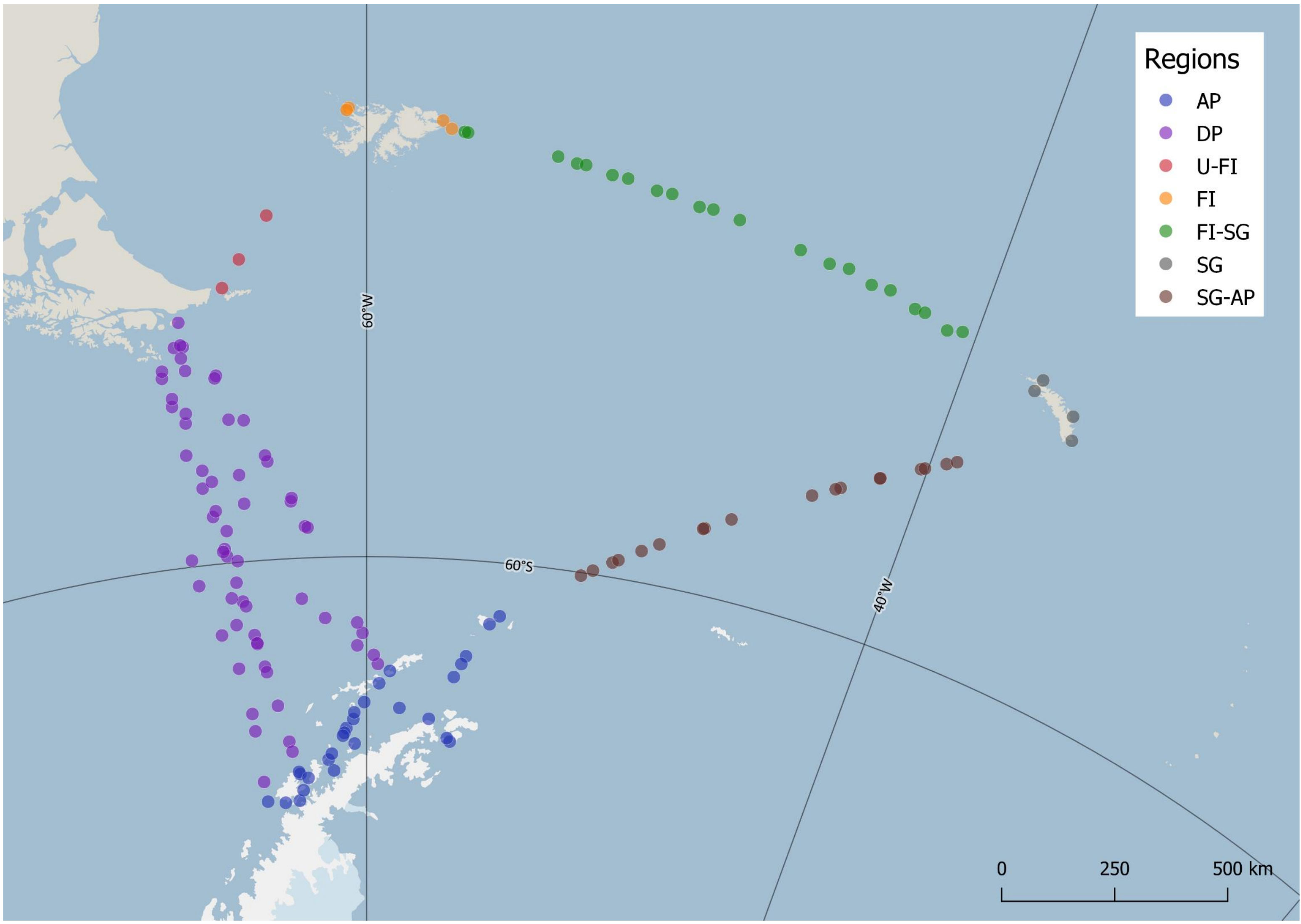
Figure 2 Study area with dots representing mean latitude and mean longitude of observations binned in 100 km intervals along the vessel tracks. Colours indicate regional division of sample units for improved visualization in Constrained Correspondence Analysis. The separated regions are the Antarctic Peninsula (AP), the Drake Passage (DP), the Falkland Islands (FI), South Georgia (SG), and the ocean areas between Ushuaia and FI (U-FI), FI and SG (FI-SG), and SG and AP (SG-AP). Limits between coastal and pelagic regions were drawn arbitrarily at 20 km from the coast, but exceptions were made around the tip of South America where three observations <20 km from land were included in DP and one in U-FI, and in the Bransfield Strait where all observations were included in AP. Map produced using Quantarctica (Matsuoka et al., 2021) and datasets therein (SCAR Antarctic Digital Database) in QGIS (QGIS.org, 2019).
Collinearity between predictors was explored through pairwise correlations with Pearson’s and Spearman’s correlation factors (Supplementary Figures S1, S2). Collinearity of |r| < 0.7 between predictors in the same model was considered acceptable (Dormann et al., 2013), and collinearity above this threshold did not occur between our predictors. Significance was assessed at α = 0.05.
2.4.1 Seabird community composition
Community composition and environmental drivers of species assemblages were explored through Constrained Correspondence Analysis (CCA) which reduces the high dimensionality in community data in the space constrained by chosen predictors to a two-dimensional approximation (Quinn & Keough, 2002; Greenacre & Primicerio, 2013). The ‘vegan’ package (v2.5-6; Oksanen et al., 2019) was used for the CCA, which was performed on square root transformed species densities to homogenize variation in abundance between species.
Because the strip-transects were irregular in both space and time, traditional tests of autocorrelation would not be effective. Hence, a restricted permutation design in the form of sequential randomization was incorporated in the analysis of variance (ANOVA) of the CCA to account for autocorrelation between consecutive sample units (Fortin & Jacquez, 2000; Anderson, 2001). Model selection was done through forward selection and backward elimination (Borcard, 2006), and VIFs (Variance Inflation Factors) were used to check for multicollinearity in model predictors.
2.4.2 Seabird species richness and density
Seabird habitat use and aggregations were explored by calculating the species richness and total seabird density observed. To minimize potential bias towards ship-associated species, we used absolute species richness (number of taxonomic groups detected, Supplementary Table S1) instead of diversity indices. The true species richness might have been higher however, as some taxonomic groups include two or more species.
Generalized Additive Models (GAM) were used to explore non-linear relationships between environmental predictors and species richness, and between environmental predictors and seabird density (total number of birds km-2). GAMs are well-suited for analysis of at-sea counts of seabirds (Clarke et al., 2003) and were used here to examine the degree to which selected environmental characteristics may influence seabird species richness and density. However, species-specific behaviors, such as ship attraction or avoidance, cause species-specific biases that all affect total density. Some caution should therefore be applied when using total density as a measure of abundance, as it is affected by the species composition within an area.
The GAMs were fitted with untransformed response data using thin plate splines. The distribution family used in the GAM for species richness was Gaussian, while negative binomial was used in the GAM for total density. Restricted Maximum Likelihood (REML) estimation was used in both models (Wood, 2011; Simpson, 2018) and covariate selection was done through null-space penalization (Wood, 2003; Wood, 2011; Wood et al., 2016). The full model for species richness was specified as
and the full model for seabird density was specified as
where s1(.) – s5(.) are smooth functions to be estimated. The model predictors are SST, the SST gradient (TG), the bathymetric slope, distance to coast (dist), and number of observation periods (strip-transects) within 100-km bins (n). Package ‘mgcv’ (v1.8-31; Wood, 2011; Wood et al., 2016) was used for fitting GAMs.
Further, latitudinal changes in species richness and seabird density were examined in relation to latitudinal variation in distance to coast, SST, and the SST gradient, by plotting the data and fitting GAM smooth curves to them. This was done separately for the eastern (Falkland Islands - Drake Passage - Antarctic Peninsula) and western (Falkland Islands - South Georgia - Antarctic Peninsula) sides of the study area (Figure 3).
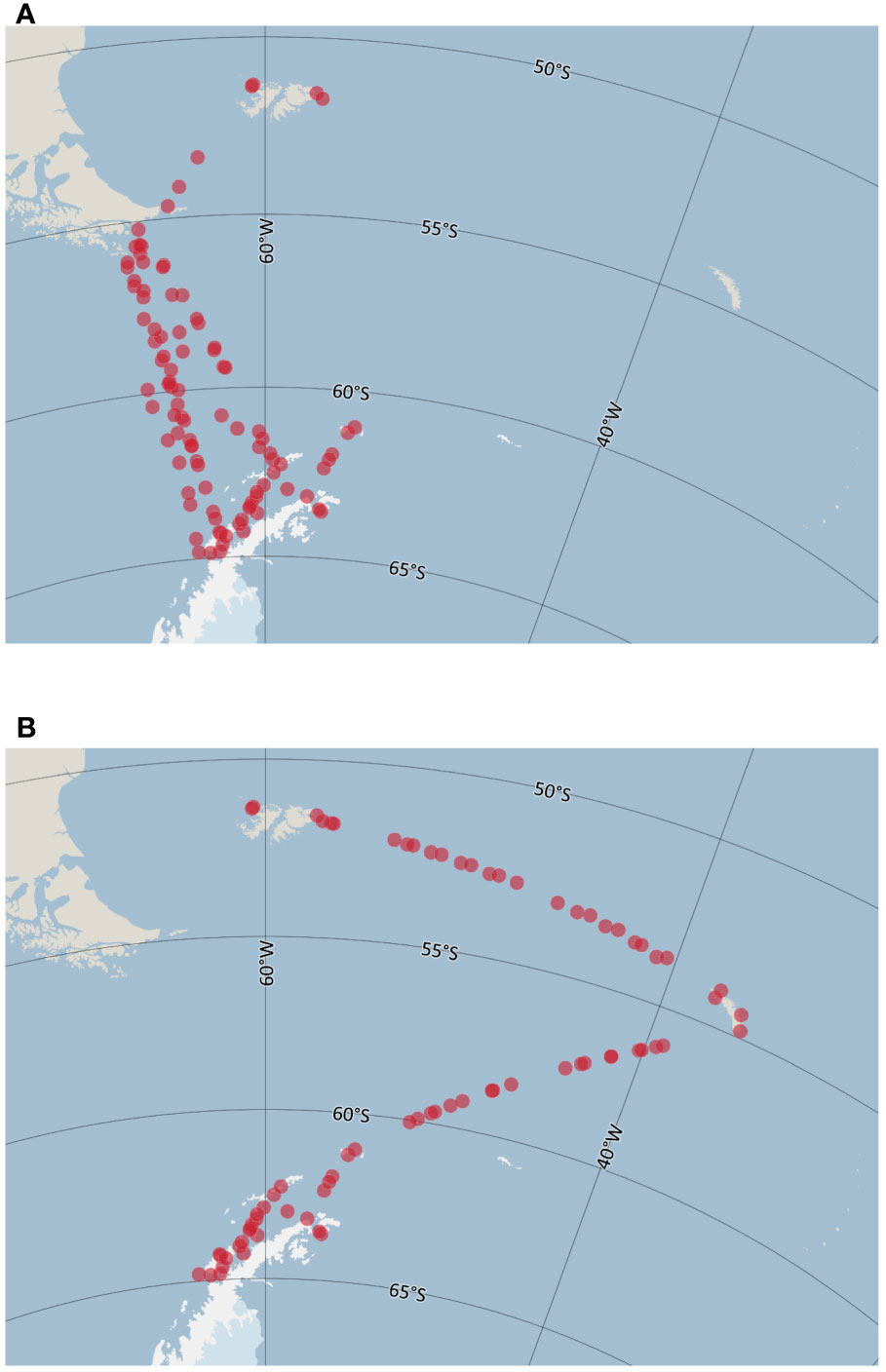
Figure 3 Sample units divided into western Scotia Sea (A) and eastern Scotia Sea (B). Maps produced using Quantarctica (Matsuoka et al., 2021) and datasets therein (SCAR Antarctic Digital Database) in QGIS (QGIS.org, 2019).
3 Results
A total of 636 strip-transects (294 on MS Midnatsol and 342 on MS Fram) covering an area of 690 km² were surveyed. Twenty-eight taxonomic groups were observed (Supplementary Table S1), of which nineteen were identified at species level. Observed species richness and total seabird density are shown for individual observations (strip-transects) in Supplementary Figures S3, S4, respectively. After removing the strip-transects counted at low and high speeds, and two observations close to South Georgia with extreme abundance of prions, 399 strip-transects were aggregated into 140 100-km bins that were included in our statistical analyses.
3.1 Seabird community composition
In the model fitted through CCA, the predictors of different species assemblages were SST (p=0.001) and distance to coast (p=0.001). Together they explained 13.8% of the variation in data (Figure 4). Both forward selection and backward elimination resulted in the same model, and the VIFs for both model predictors were ∼1.0. The horizontal CCA1 axis mainly represents changing SST and thus a latitudinal gradient in community composition, while the vertical CCA2 axis largely represents a coastal-oceanic gradient, separating breeding coastal species from breeding oceanic species that can travel farther in search for food. Seabird communities appear in regional groups in the CCA plot, highlighting the spatial segregation of seabird species assemblages. In particular, communities in the AP and Falkland Islands stood out as substantially different from the others. The AP in the south end of the study area was characterized by ice-associated species, while the Falkland Islands which are situated north of the Subantarctic Front formed a distinct group. For the open ocean seabird communities, there was a latitudinal change in species assemblages between the northern and southern SS.
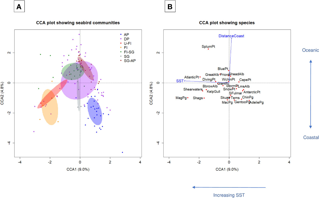
Figure 4 Constrained Correspondence Analysis (CCA) ordination biplot of axes 1 and 2 of seabird communities. Panel (A) shows seabird communities (binned strip-transect observations) as dots with colour indicating region: Antarctic Peninsula (AP), the Drake Passage (DP), the Falkland Islands (FI), South Georgia (SG), and the ocean areas between Ushuaia and FI (U-FI), FI and SG (FI-SG), and SG and AP (SG-AP). Ellipses represent standard deviations of sample units inside each region. Panel (B) shows species (red dots) and significant predictors (blue arrows). The significant predictors (sea surface temperature (SST) and distance to coast (DistanceCoast)) explained 13.8% of the total variation in community composition.
Seabird communities over temperate and Subantarctic waters north of the Polar Front were dominated by black-browed (Thalassarche melanophrys) and great albatrosses (Diomedea spp.), shearwaters (Puffinus spp.), Atlantic petrel (Pterodroma incerta), shags (Phalocrocorax spp.), and magellanic penguin (Spheniscus magellanicus), whose diet consists mainly of cephalopods and fish (Supplementary Table S1). Communities over Antarctic waters south of the Polar Front, where krill is abundant, were characterized by planktivores such as Adélie (Pygoscelis adeliae) and chinstrap penguins (P. antarcticus), storm petrels (Oceanites oceanicus and Fregetta spp.), blue petrel (Halobaena caerulea), and prions (Pachyptila spp.). Snow (Pagodroma nivea) and Antarctic petrels (Thalassoica antarctica) are mixed feeders that are adapted to foraging in pack ice where they find less competition (Griffiths et al., 1982; Ainley et al., 1993; Ainley et al., 1994) and were primarily observed in the AP region. Skuas (Catharacta spp.) were observed close to penguin colonies, where they feed on penguin eggs and chicks in the austral summer (Shirihai, 2007).
3.2 Seabird species richness
The best supported GAM of species richness included the predictors SST (p=0.019), SST gradient (p<0.001), distance to coast (p=0.031), and number of observation periods within 100-km bins (p<0.001), and this model explained 43.9% of the total variation in the data (Figure 5). The residual plots of the model look satisfactory (Supplementary Figure S5), and residual autocorrelation was low and consequently not considered a problem (Supplementary Figure S6). Generally, seabird species richness peaked at surface water temperatures around 3°C and decreased slightly with distance from coast (Figure 5). The number of species observed increased with observation effort (number of observation periods within 100-km bins), as expected. The effect of the SST gradient on species richness did not show a general trend, but low and high values were associated with relatively higher species richness while medium values were associated with lower species richness (Figure 5).
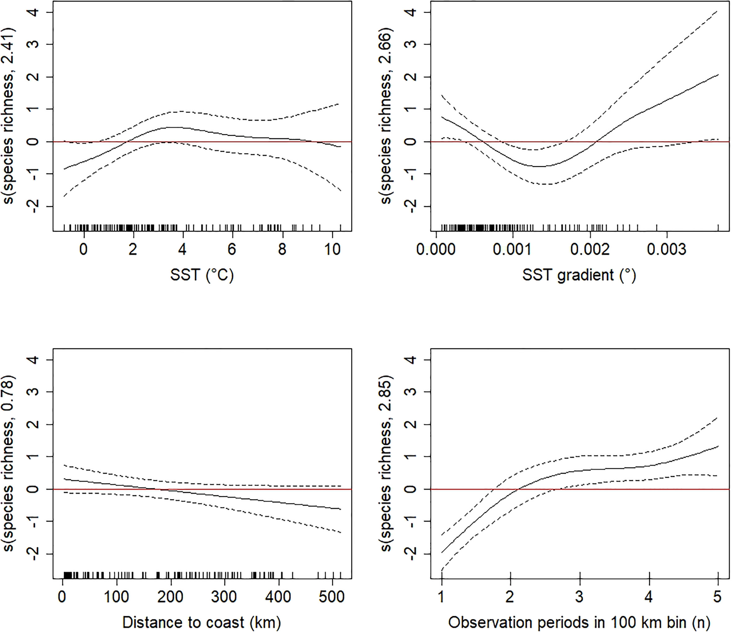
Figure 5 Generalized Additive Model smooth terms (s, linear predictor scale) of species richness as a function of significant explanatory variables (sea surface temperature (SST), SST gradient, distance to coast, and number of observation periods) with null space penalization. The dotted lines represent the 95% confidence intervals. Estimated degrees of freedom (edf) are given in the y-axis label.
Latitudinal variation in species richness on the western and eastern sides of the Scotia Sea are shown in Figures 6, 7, respectively, together with variation in distance to coast, SST, the SST gradient, and seabird density. Except for a peak north of South Georgia, species richness did not vary considerably with latitude on the western nor the eastern side of the Scotia Sea. An elevated SST gradient was found close to land masses and at the Polar Front in the Drake Passage.
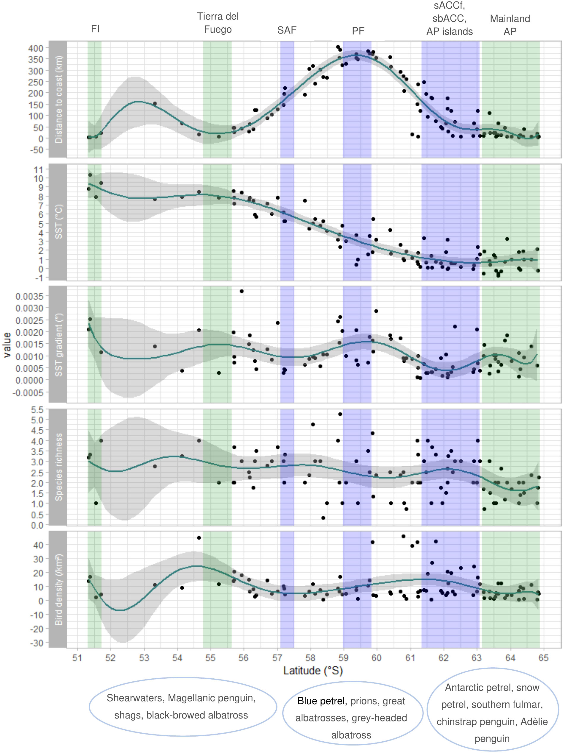
Figure 6 Latitudinal change in distance to coast, SST, SST gradient, species richness, and seabird density for sample units in the western Scotia Sea between the Falkland Islands and Antarctic Peninsula. GAM smoothed curves were fitted to data and are shown together with 95% confidence intervals. Coloured columns mark regions characterised by land (green) or/and the mean positions of oceanographic fronts (blue) named above the plot. These are the Falkland Islands (FI), Tierra del Fuego at the southern tip of South America, the Subantarctic front (SAF), Polar front (PF), southern Antarctic Circumpolar Current front (sACCf) and the southern boundary of the Antarctic Circumpolar Current (sbACC) together with islands north of the Antarctic Peninsula (AP), and mainland AP. Characteristic species of regional communities are named under the latitudes corresponding to their spatial distribution in western Scotia Sea. Figure produced using R package ‘ggplot2’ (Wickham, 2016).
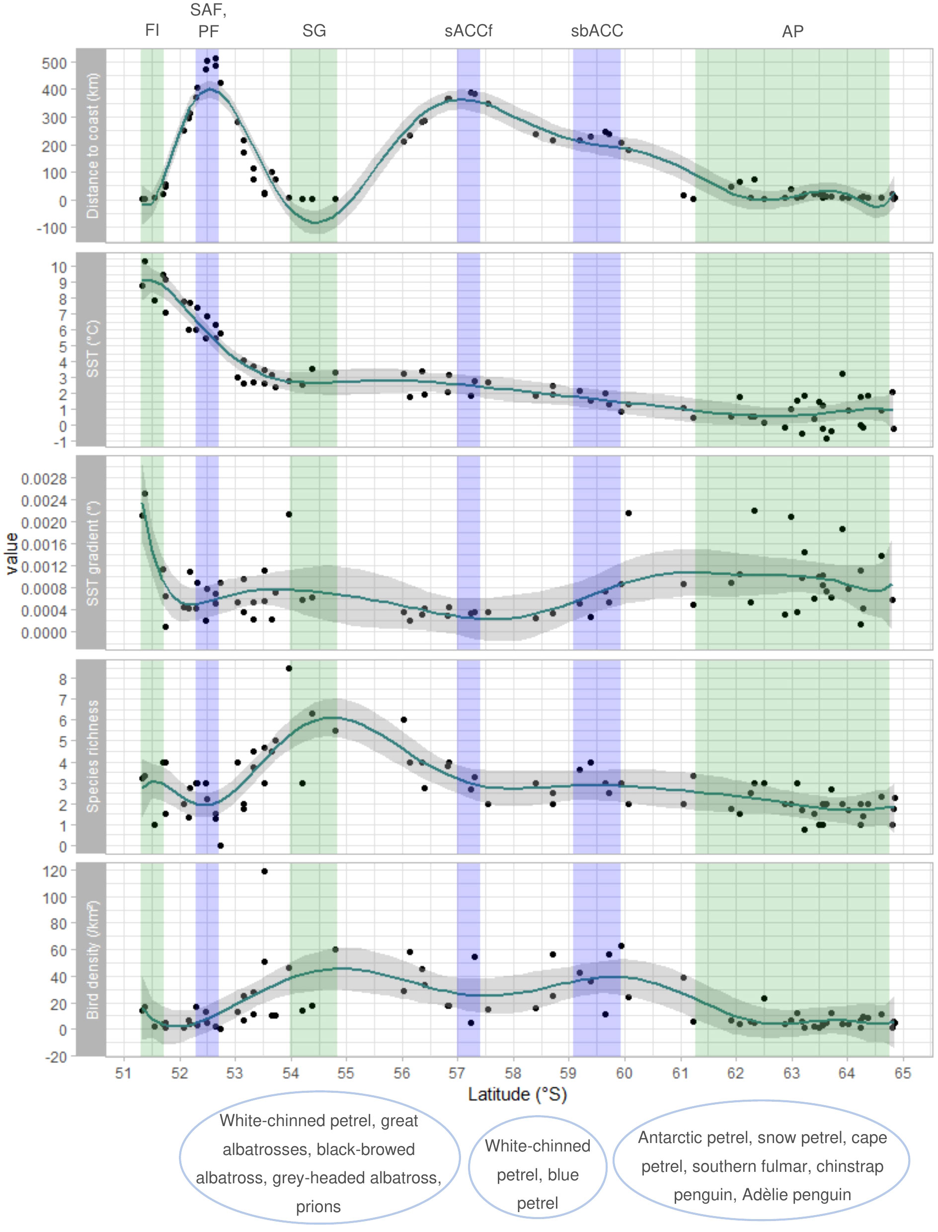
Figure 7 Latitudinal change in distance to coast, SST, SST gradient, species richness, and seabird density for sample units in the eastern Scotia Sea between the Falkland Islands, South Georgia, and Antarctic Peninsula. GAM smoothed curves were fitted to data and are shown together with 95% confidence intervals. Coloured columns mark regions characterised by land (green) or the mean positions of oceanographic fronts (blue) named above the plot. These are the Falkland Islands (FI), Subantarctic Front (SAF) and Polar front (PF), South Georgia (SG), southern Antarctic Circumpolar Current front (sACCf), the southern boundary of the Antarctic Circumpolar Current (sbACC), and the Antarctic Peninsula (AP; mainland and islands). Characteristic species of regional communities are named under the latitudes corresponding to their spatial distribution in the eastern Scotia Sea. Figure produced using R package ‘ggplot2’ (Wickham, 2016).
3.3 Seabird density
The best supported GAM of seabird density included the predictors SST (p<0.001) and bathymetric slope (p<0.001), and this model explained 21.1% of the total variation in the data (Figure 8). The residual plots of the model look satisfactory (Supplementary Figure S7), but there was slight autocorrelation in the residuals (Supplementary Figure S8). Generally, seabird density peaked at surface water temperatures around 2-3°C, and lower seabird densities were associated with a higher bathymetric slope.
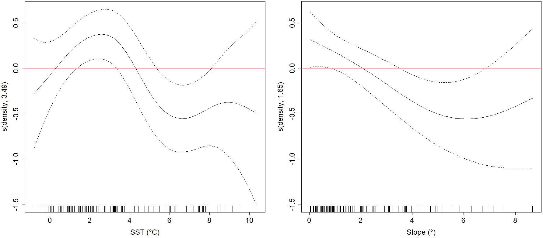
Figure 8 Generalized Additive Model smooth terms (s, linear predictor scale) of total densities as a function of significant explanatory variables (sea surface temperature (SST) and bathymetric slope (slope)) with null space penalization. The dotted lines represent the 95% confidence intervals. Estimated degrees of freedom (edf) are given in the y-axis label.
Latitudinal variation in seabird density on the western and eastern sides of the Scotia Sea are shown in Figures 6, 7, respectively, together with variation in distance to coast, SST, the SST gradient, and species richness. Highest seabird densities were found close to South Georgia and at the sbACC on the eastern side of the study area.
4 Discussion
Our study suggests that the Scotia Sea (SS) and Antarctic Peninsula (AP) system is characterized more clearly by oceanographic separation of seabird communities (Figure 4) than by seabird aggregations in space, supporting the findings of Ribic et al. (2011). Similar results have been described by Abrams (1985) in the African sector of the Southern Ocean. South Georgia provides an exception to this pattern, standing out with relatively higher seabird abundance and species richness compared to the rest of the area in the breeding season. Species assemblages differed between the AP, South Georgia, and Falkland Islands, while the different ocean areas (e.g., Drake Passage, Falklands to South Georgia [Figure 2]) had varying degrees of overlap generally characterized with a gradual north-south cline in species assemblages. Coastal communities in South Georgia resembled those in open-ocean areas, presumably because of the many oceanic species that breed there (Shirihai, 2007). Seabird communities and species distributions were structured along geographical gradients, supposedly reflecting the distribution of prey species, breeding sites and species-specific biogeographical history and physiological and behavioral adaptations (Pocklington, 1979; Wahl et al., 1989; Ainley et al., 1994). SST and distance to coast were the most important predictors of species assemblages, reflecting species-specific biogeography and life history traits. The results from this study are consistent with results from the AP (Warwick-Evans et al., 2021), where SST and depth accounted for most variation in seabird distribution, as well as results from other locations such as the Southeast Pacific (Serratosa et al., 2020), where SST and an oceanic-coastal gradient were important predictors of seabird community composition. Areas of high variability in sea surface temperature or bathymetry, indicative of oceanographic fronts and continental slopes respectively, were not predictive of elevated seabird abundance.
4.1 Different water masses, different communities
Predator communities are associated with specific ranges of geographical gradients through their diets and physiological and behavioral adaptations, and predator-habitat relationships generally reflect predator-prey relationships (Griffiths et al., 1982; Ainley et al., 1993; Ballance, 2007; Fauchald et al., 2011a). Sea surface temperature (SST) has been described as the most important predictor of marine biodiversity on a global scale (Tittensor et al., 2010) and was a strong overall predictor of seabird distribution in this study. Ocean surface temperature typically varies between water masses and gradients arise where water masses converge, creating oceanic habitats with physical characteristics occupied by different assemblages of prey species (Pocklington, 1979; Wahl et al., 1989; Jungblut et al., 2017; Chapman et al., 2020). Water characteristics such as temperature, salinity, and nutrient concentrations in the Southern Ocean show large latitudinal gradients, dividing the ocean into biogeographical zones (Grant et al., 2006). Our results show how different seabird communities inhabit waters that lie within specific ranges of a temperature gradient, corresponding to different water masses in the Scotia Sea. Seabird abundance and species richness also vary between water masses, presumably because of differences in productivity between oceanographic regions. Seabird communities over temperate and Subantarctic waters north of the Polar Front were dominated by seabirds feeding mainly on cephalopods and fish, while communities over Antarctic waters south of the Polar Front were dominated by planktivores and species adapted to foraging in pack ice. These results support earlier studies that found an association between seabird communities consisting of species with similar dietary preferences and water masses inhabited by preferred prey (Abrams, 1985; Abrams & Miller, 1986; Hunt et al., 1990; Joiris, 1991), as well as studies underlining the importance of niche segregation for the spatial distribution of seabirds. Interspecific interactions, such as competition and facilitation, and species-specific energetic constraints are factors that cause different seabird species to respond differently to the distribution of their prey (Ballance et al., 1997; Ballance, 2007; Fauchald et al., 2011a; Veit & Harrison, 2017). Interspecific competition and energetic constraints structure seabird communities along a productivity gradient (Ballance et al., 1997), while local enhancement and facilitation associate surface feeding species that have a relatively low energetic cost of flight (and therefore low cost of search behavior) with diving species that drive prey up to the surface (Veit & Harrison, 2017). Seabird species are consequently found in niches formed by the interaction between dietary preferences and interspecific interactions such as competition and facilitation. For instance, the white-chinned petrel (Procellaria aequinoctialis), and black-browed, grey-headed (T. chrysostoma), and wandering albatrosses (Diomedea exulans), have been suggested to outcompete the light-mantled sooty albatross (Phoebetria palpebrata) on foraging grounds close to breeding colonies in SG, thereby forcing it to utilize more distant areas for foraging (Phillips et al., 2005). We indeed observed light-mantled sooty albatrosses generally in more Antarctic environments and further from the breeding colonies in SG than other albatross species, possibly as a consequence of spatial segregation in foraging areas between sympatric species in the same foraging guild.
4.2 The coastal-oceanic gradient
The coastal-oceanic gradient is another important factor affecting prey species present through gradients in productivity, bathymetry, and water characteristics (Doty & Oguri, 1956; Abrams & Miller, 1986), contributing to the differences in seabird assemblages between the oceanic and coastal habitats described in this study. Our survey was conducted during the early and mid-austral summer, when many seabird species breed. Breeding poses a spatial constraint on seabirds (Gaston, 2004; Amorim et al., 2009); the need to return to land to take turns with the partner for brooding duties at the nest constrains how far and for how long adult birds can forage at sea. These restrictions lead to higher densities of some bird species in coastal waters (Abrams & Miller, 1986), a pattern detected in this study as a negative relationship between seabird species richness and distance from coast, as well as a negative but not statistically significant relationship between seabird density and distance from coast. For example, large numbers of oceanic species like grey-headed albatross and white-chinned petrel were observed in the coastal waters off South Georgia.
4.3 Oceanographic fronts
In the open ocean, strong gradients in SST are generally indicative of oceanographic fronts, which might act in two ways in shaping seabird distribution. First, as productive areas they can be associated with an elevated abundance of seabirds and other higher-level predators (Wahl et al., 1989; Bost et al., 2009) and second, they can act as avifaunal boundaries, separating different species assemblages (Pocklington, 1979; Wahl et al., 1989), as has been described for the Polar Front and the southern boundary of the Antarctic Circumpolar Current (sbACC) (Ribic et al., 2011). Ribic et al. (2011) found increased abundances of a few species, including diving petrels and blue petrel, at the Polar Front and the sbACC, but the fronts’ effect as boundaries for differing species assemblages was more pronounced. Seabirds breeding in the South Shetland Islands have been shown to use the sbACC as an important feeding ground (Santora & Veit, 2013), pointing towards both a possible aggregating effect of the sbACC, and its possible role as a boundary for AP species in the breeding season. The role of fronts as boundaries could explain the high importance of SST for community composition and the low effect of temperature gradient in our analyses. The SST gradient did not manage to capture an effect of fronts on oceanic communities, and the effect of the SST gradient on seabird abundance did not show a general trend contrary to results from for example Serratosa et al. (2020). Instead, relatively higher densities were associated with low and high temperature gradients, while medium gradient values were associated with relatively lower seabird density. While there was no statistical support for seabird species richness increasing with an increasing temperature gradient, and its effect on seabird density was unclear, there was a general peak in density and species richness around SSTs of 3°C. These temperatures are usually associated with waters around the Polar Front and around South Georgia. A possible explanation for the lack of effect of the SST gradient is that a frontal temperature gradient might not always be detectable at the surface (Chapman et al., 2020). The role of fronts as areas of increased productivity might also be less important in summer when food is abundant in the SS (Ribic et al., 2011), or because breeding birds experience stronger constraints on their foraging range and might not be able to reach fronts. The effect of restricted foraging range likely explains the lack of effect of fronts lying far from land, notably the Polar front.
4.4 Upwelling areas
Other studies have shown a positive association of seabird abundance with areas of coastal upwelling, such as in the Eastern South Pacific Ocean (Serratosa et al., 2020). Interestingly, the density of seabirds in this study appeared to decline in relation to higher bathymetric slopes which are typically associated with coastal upwelling. Potentially, this trend may be related to the overall lower species richness in the topographically complex AP compared to the sub-Antarctic areas (Hindell et al., 2020). Seabird communities in the coastal AP region were associated with a variable bathymetry (Figure 4), which likely reflects the deep basins of Bransfield Strait and the deep fjords around coasts of the AP. The highest seabird densities were found in waters around South Georgia, which lies on a large plateau. Further, a smaller number of flying seabird species in the AP might reduce the flux of birds within strip-transects compared to other areas, biasing total bird counts towards sub-Antarctic areas. Also, penguins are a dominant group in the AP and have been suggested to dive as a response to ships (Jehl, 1974, as cited in Tasker et al., 1984). On the ship transects between land masses, strip-transects situated at continental slopes were few, which may have reduced our ability to detect any effect of slope on seabird abundance in the oceanic environment.
4.5 Limitations
Some biases in our data were expected due to the methodology used. Species counts are potentially inflated or deflated due to species-specific responses to the ship, mainly ship attraction or avoidance (e.g., Hyrenbach, 2001). Species such as giant petrels, cape petrel and black-browed albatross are ship-followers, and their abundances are therefore easily overestimated. The fact that many flying birds travel faster than the ship increases their chance of entering the strip-transect relative to birds sitting on the sea surface (Spear et al., 1992; van Franeker, 1994). The flux of flying birds in the strip-transect is hence a function of their speed relative to the speed of the vessel. Flux can be corrected for using a snapshot method (Tasker et al., 1984), where all flying birds are counted regularly in instantaneous counts. Here, we counted all birds, including flying birds, using a continuous method. This likely introduces bias from ship attraction and bird flux in our results. Using cruise vessels as observation platforms, we were not able to control vessel speed. This might cause variation in flux between strip-transects and we excluded strip-transects counted in low and high speeds from the analyses in order to reduce potential bias caused by vessel speed. It is also worth noting that species richness in some of our strip-transects might have been underestimated as species that were hard to identify at sea were grouped together. For example, sympatric species of storm petrels are found in the AP and sympatric species of prions are found in South Georgia and the Falkland Islands (Shirihai, 2007; Clarke et al., 2012). We recommend including snapshot counts to control for the flux of flying birds in strip-transects. To reduce variance associated with the different number of observation periods in each 100 km segment, and to increase the precision of mean counts used for data analysis, we further recommend more frequent observation periods on future surveys.
4.6 Cruise vessels as opportunistic sampling platforms
Ships of opportunity give the possibility to cover large areas and large-scale environmental gradients. This is of paramount importance for detecting seabird communities’ responses to environmental change. In the case of our study, the routes allowed a representative dataset of the Scotia Sea and northern Antarctic Peninsula to be collected by crossing all biogeographical regions in the study area (Grant et al., 2006) and covering both oceanic and coastal areas (though not the coasts of South Orkney and South Sandwich Islands). Nature-based tourist cruises usually ensure coverage of biodiversity hotspots. Coastal and hotspot areas are of particular interest for tourist cruises, and our effort was hence concentrated towards these areas. This increases data precision in coastal areas and areas with high biodiversity, which is an advantage as these are the most important areas for conservation monitoring. However, the predetermined routes of cruise vessels, strongly concentrated to specific regions, leave vast areas unsampled. Large parts of the Southern Ocean and most coasts of Antarctica are never visited by cruise ships. Areas outside the reach of cruise vessels need to be covered by research surveys with the possibility for a more representative sampling design, or possibly sampled opportunistically by observers onboard supply vessels or fishing ships going to some of these areas. We nevertheless argue that cruise vessels and other opportunistic sampling platforms provide opportunities for the collection of data (e.g., repeated surveys within and between years) that can augment our understanding of seabird ecology and ecosystem change when combined with data collected on dedicated research surveys. Johannessen et al. (2022) and Henderson et al. (2023) provide examples of the use of cruise ships in studies on baleen whales in our study area.
4.7 Implications for ecosystem monitoring and management
Data on seabird distribution are important for ecosystem monitoring, and for conservation efforts like the establishment of MPAs and spatial and temporal management of fisheries. Marine predator distribution studies have seen a shift from an area-centered approach using ship surveys towards a population-centered approach using tracking data (Hindell et al., 2020; Fauchald et al., 2021). However, tracking data typically do not represent all species, populations, demographic groups, and individuals using the studied area, and ship surveys continue to be an important method for validation and completion of tracking data (Fauchald et al., 2021). In the 1980s and 1990s, chinstrap (Pygoscelis antarcticus) and Adélie penguins (P. adeliae) were the most commonly observed penguin species in the Bransfield Strait region (Hunt et al., 1990; Hunt et al., 1994). We noticed a change in the relative abundances of pygoscelid penguins, previously described by Lynch et al. (2012), observing more gentoo penguins (P. papua) than chinstrap or Adélie penguins in the area. Studies like ours provide information on the distribution of seabirds for future comparisons assessing ecosystem change, for which community-level data are particularly useful. Models that incorporate multiple species and predictors can be effective in revealing complex relationships, since they consider multiple responses inside the same community (Reid et al., 2005; Piatt et al., 2007; Hindell et al., 2020). Considering community-level responses is important in making meaningful management decisions and networks of MPAs should be designed in a way that they consider the diversity of communities as well as future change in species distribution (Hindell et al., 2020).
5 Conclusions
Our results show differing species assemblages between distinct oceanographic zones around the Scotia Sea, demonstrating species’ association with specific habitat characteristics. In addition, they underline the importance of distance to colonies on land for seabird space use in the breeding season. The type of data presented here, collected onboard platform of opportunity cruise vessels, can be a valuable addition to research cruises and tracking data. Large data sets are needed to cover the spatial and temporal scales relevant to seabirds and regularly conducted multi-species seabird surveys are paramount in detecting distributional changes. Effective management and conservation rely on knowledge of species distribution and habitat use, and become increasingly relevant with ongoing climate change, krill harvesting, and increasing interactions with recovering populations of marine mammals. The results from this study can serve as a baseline for future studies aiming to assess seasonal and interannual variation and long-term changes in seabird distribution throughout the Antarctic Peninsula and Scotia Sea.
Data availability statement
The datasets generated and analyzed for this study can be found at https://doi.org/10.5281/zenodo.8313941 (Ollus et al., 2023).
Ethics statement
Ethical review and approval was not required for the study on animals in accordance with the local legislation and institutional requirements.
Author contributions
This study was designed by UL, MB, AL, LM, KG, and WO, and supervised by UL, MB and AL. Data was collected by VO, JJ, LM, KG, and WO. Data analysis, interpretation and writing of the original manuscript was led by VO and supported by UL, MB, AL, and PF. All authors contributed to manuscript revision, read, and approved the submitted version.
Funding
This research was funded by UiT The Arctic University of Norway and the Norwegian Polar Institute. Open access publishing was funded by UiT The Arctic University of Norway.
Acknowledgments
The authors thank Dr Verena Meraldi and Tudor Morgan of Hurtigruten Expeditions for providing field and logistical support. Thanks also to the officers, crews, and expedition teams for their hospitality onboard MS Midnatsol and MS Fram. Special thanks to Dr Raul Primicerio for statistical guidance in permutation design for the Constrained Correspondence Analysis, and to Dr Tone Reiertsen for insightful comments on earlier versions of the manuscript. Preliminary results from this study were published in the master’s thesis of Ollus (2021).
Conflict of interest
The authors declare that the research was conducted in the absence of any commercial or financial relationships that could be construed as a potential conflict of interest.
Publisher’s note
All claims expressed in this article are solely those of the authors and do not necessarily represent those of their affiliated organizations, or those of the publisher, the editors and the reviewers. Any product that may be evaluated in this article, or claim that may be made by its manufacturer, is not guaranteed or endorsed by the publisher.
Supplementary material
The Supplementary Material for this article can be found online at: https://www.frontiersin.org/articles/10.3389/fmars.2023.1233820/full#supplementary-material
References
Abrams R. W. (1985). Environmental determinants of pelagic seabird distribution in the African sector of the Southern Ocean. J. Biogeogr. 12, 473–492. doi: 10.2307/2844955
Abrams R. W., Miller D. G. M. (1986). The distribution of pelagic seabirds in relation to the oceanic environment of Gough Island. South Afr. J. Mar. Sci. 4 (1), 125–137. doi: 10.2989/025776186784461666
Ainley D. G., Ribic C. A., Fraser W. R. (1994). Ecological structure among migrant and resident seabirds of the Scotia-Weddell Confluence region. J. Anim. Ecol. 63, 347–364. doi: 10.2307/5553
Ainley D. G., Ribic C. A., Spear L. B. (1993). Species-habitat relationships among antarctic seabirds: A function of physical or biological factors? Condor. 95, 806–816. doi: 10.2307/1369419
Alvito P. M., Rosa R., Phillips R. A., Cherel Y., Ceia F., Guerreiro M., et al. (2015). Cephalopods in the diet of nonbreeding black-browed and grey-headed albatrosses from South Georgia. Polar Biol. 38, 631–641. doi: 10.1007/s00300-014-1626-3
Amante C., Eakins B. W. (2009) ETOPO1 1 Arc-Minute Global Relief Model: Procedures, Data Sources and Analysis. NOAA Technical Memorandum NESDIS NGDC-24 (National Geophysical Data Center, NOAA) (Accessed 30 Sep 2020).
Amorim P., Figueiredo M., Machete M., Morato T., Martins A., Serrão Santos R. (2009). Spatial variability of seabird distribution associated with environmental factors: a case study of marine Important Bird Areas in the Azores. ICES J. Mar. Sci. 66 (1), 29–40. doi: 10.1093/icesjms/fsn175
Anderson M. J. (2001). Permutation tests for univariate or multivariate analysis of variance and regression. Can. J. Fisheries Aquat. Sci. 58 (3), 626–639. doi: 10.1139/f01-004
Arndt J. E., Schenke H. W., Jakobsson M., Nitsche F., Buys G., Goleby B., et al. (2013). The International Bathymetric Chart of the Southern Ocean (IBCSO) Version 1.0 - A new bathymetric compilation covering circum-Antarctic waters. Geophys. Res. Lett. 40, 3111–3117. doi: 10.1002/grl.50413
Atkinson A., Hill S. L., Pakhomov E. A., Siegel V., Reiss C. S., Loeb V. J., et al. (2019). Krill (Euphausia superba) distribution contracts southward during rapid regional warming. Nat. Climate Change 9, 142–147. doi: 10.1038/s41558-018-0370-z
Atkinson A., Siegel V., Pakhomov E., Rothery P. (2004). Long-term decline in krill stock and increase in salps within the Southern Ocean. Nature 432 (7013), 100–103. doi: 10.1038/nature02996
Atkinson A., Whitehouse M. J., Priddle J., Cripps G. C., Ward P., Brandon M. A. (2001). South Georgia, Antarctica: a productive, cold water, pelagic ecosystem. Mar. Ecol. Prog. Ser. 216, 279–308. doi: 10.3354/meps216279
Baines M., Kelly N., Reichelt M., Lacey C., Pinder S., Fielding S., et al. (2021). Population abundance of recovering humpback whales Megaptera novaeangliae and other baleen whales in the Scotia Arc, South Atlantic. Mar. Ecol. Prog. Ser. 676, 77–94. doi: 10.3354/meps13849
Ballance L. T., Pitman R. L., Reilly S. B. (1997). Seabird community structure along a productivity gradient: importance of competition and energetic constraint. Ecology 78, 1502–1518. doi: 10.1890/0012-9658(1997)078[1502:SCSAAP]2.0.CO;2
Barbraud C., Rolland V., Jenouvrier S., Nevoux M., Delord K., Weimerskirch H. (2012). Effects of climate change and fisheries bycatch on Southern Ocean seabirds: a review. Mar. Ecol. Prog. Ser. 454, 285–307. doi: 10.3354/meps09616
Barrera-Oro E. (2002). The role of fish in the Antarctic marine food web: differences between inshore and offshore waters in the southern Scotia Arc and west Antarctic Peninsula. Antarctic Sci. 14 (4), 293–309. doi: 10.1017/S0954102002000111
Bertrand S., Joo R., Arbulu Smet C., Tremblay Y., Barbraud C., Weimerskirch H. (2012). Local depletion by a fishery can affect seabird foraging. J. Appl. Ecol. 49, 1168–1177. doi: 10.1111/j.1365-2664.2012.02190.x
Bestley S., Ropert-Coudert Y., Bengtson Nash S., Brooks C. M., Cotté C., Dewar M., et al. (2020). Marine ecosystem assessment for the Southern ocean: birds and marine mammals in a changing climate. Front. Ecol. Evol. 8, 566936. doi: 10.3389/fevo.2020.566936
Bindoff N. L., Cheung W. W. L., Kairo J. G., Arístegui J., Guinder V. A., Hallberg R., et al. (2019). “Changing ocean, marine ecosystems, and dependent communities,” in IPCC special report on the ocean and cryosphere in a changing climate. Eds. Pörtner H.-O., Roberts D. C., Masson-Delmotte V., Zhai P., Tignor M., Poloczanska E., et al (Cambridge, UK and New York, NY, USA: Cambridge University Press), 447–587.
Bolduc F., Fifield D. A. (2017). Seabirds at-sea surveys: the line-transect method outperforms the point-transect alternative. Open Ornithol. J. 10, 42–52. doi: 10.2174/1874453201710010042
Bost C. A., Cotté C., Bailleul F., Cherel Y., Charrassin J. B., Guinet C., et al. (2009). The importance of oceanic fronts to marine birds and mammals of the southern oceans. J. Mar. Syst. 78, 363–376. doi: 10.1016/j.jmarsys.2008.11.022
CCAMLR (2019). Report of the thirty-eighth meeting of the scientific committee, Hobart, Australia, 21 to 25 October 2019 (Hobart, Australia: CCAMLR).
Chapman C. C., Lea M. A., Meyer A., Sallée J. B., Hindell M. (2020). Defining Southern Ocean fronts and their influence on biological and physical processes in a changing climate. Nat. Climate Change 10 (3), 209–219. doi: 10.1038/s41558-020-0705-4
Cherel Y., Fontaine C., Richard P., Labatc J. P. (2010). Isotopic niches and trophic levels of myctophid fishes and their predators in the Southern Ocean. Limnol. oceanogr. 55 (1), 324–332. doi: 10.4319/lo.2010.55.1.0324
Chown S. L., Brooks C. M. (2019). The state and future of Antarctic environments in a global context. Annu. Rev. Environ. Resour. 44, 1–30. doi: 10.1146/annurev-environ-101718-033236
Clarke A., Croxall J. P., Poncet S., Martin A. R., Burton R. (2012). Important bird areas: South Georgia. Br. Birds 105, 118–144.
Clarke E. D., Spear L. B., McCracken M. L., Marques F. F. C., Borchers D. L., Buckland S. T., et al. (2003). Validating the use of generalized additive models and at-sea surveys to estimate size and temporal trends of seabird populations. J. Appl. Ecol. 40, 278–292. doi: 10.1046/j.1365-2664.2003.00802.x
Dormann C. F., Elith J., Bacher S., Carré G. C. G., García Márquez J. R., Gruber B., et al. (2013). Collinearity: a review of methods to deal with it and a simulation study evaluating their performance. Ecography 36 (1), 27–46. doi: 10.1111/j.1600-0587.2012.07348.x
Doty M. S., Oguri M. (1956). The island mass effect. ICES J. Mar. Sci. 22 (1), 33–37. doi: 10.1093/icesjms/22.1.33
Egevang C., Stenhouse I. J., Phillips R. A., Petersen A., Fox J. W., Silk J. R. (2010). Tracking of Arctic terns Sterna paradisaea reveals longest animal migration. Proc. Natl. Acad. Sci. 107 (5), 2078–2081. doi: 10.1073/pnas.0909493107
Enticott J. W. (1986). Associations between seabirds and cetaceans in the African Sector of the Southern Ocean. South Afr. J. Antarctic Res. 16, 25–28.
European Seabirds At Sea (ESAS) (2022). ICES (Copenhagen, Denmark: ICES). Available at: https://esas.ices.dk.
Fauchald P., Erikstad K. E., Skarsfjord H. (2000). Scale-dependent predator-prey interactions: the hierarchical spatial distribution of seabirds and prey. Ecology 81 (3), 773–783. doi: 10.1890/0012-9658(2000)081[0773:SDPPIT]2.0.CO;2
Fauchald P., Skov H., Skern-Mauritzen M., Hausner V. H., Johns D., Tveraa T. (2011a). Scale-dependent response diversity of seabirds to prey in the North Sea. Ecology 92, 228–239. doi: 10.1890/10-0818.1
Fauchald P., Tarroux A., Amélineau F., Bråthen V. S., Descamps S., Ekker M., et al. (2021). Year-round distribution of Northeast Atlantic seabird populations: applications for population management and marine spatial planning. Mar. Ecol. Prog. Ser. 676, 255–276. doi: 10.3354/meps13854
Fauchald P., Ziryanov S. V., Borkin I. V., Strøm H., Barrett R. T. (2011b). “Seabirds,” in The Barents Sea. Ecosystem, resources, management. Half a century of Russian-Norwegian cooperation. Eds. Jakobsen T., Ozhigin V. K. (Trondheim: Tapir Academic Press), 373–394.
Fortin M. J., Jacquez G. M. (2000). Randomization tests and spatially auto-correlated data. Bull. Ecol. Soc. America 81 (3), 201–205. https://www.jstor.org/stable/20168439
Gaston A. J. (2004). “Breeding, coloniality and its consequences,” in Seabirds: a natural history (Poyser Monographs). Ed. Gaston A. J. (London: Poyser), 142–161.
Gillespie D. M., Leaper R., Gordon J. C. D., Macleod K. (2010). A semi-automated, integrated, data collection system for line transect surveys. J. Cetacean Res. Manage. 11, 217–227. doi: 10.47536/jcrm.v11i3.601
González-Solís J., Shaffer S. A. (2009). Introduction and synthesis: spatial ecology of seabirds at sea. Mar. Ecol. Prog. Ser. 391, 117–120. doi: 10.3354/meps08282
Goyert H., Gardner B., Sollmann R., Veit R., Gilbert A., Connelly E., et al. (2016). Predicting the offshore distribution and abundance of marine birds with a hierarchical community distance sampling model. Ecol. Appl. 26 (6), 1797–1815. doi: 10.1890/15-1955.1
Grant S., Constable A., Raymond B., Doust S. (2006). Bioregionalisation of the Southern ocean: report of experts workshop, Hobart, September 2006 (Hobart, Australia: WWF-Australia and ACE CRC).
Greenacre M., Primicerio R. (2013). Multivariate analysis of ecological data (Bilbao, Spain: Fundación BBVA, Bilbao).
Griffiths A. M. (1982). Observations of pelagic seabirds feeding in the African sector of the Southern Ocean. Cormorant 10, 9–14.
Griffiths A. M., Siegfried W. R., Abrams R. W. (1982). Ecological structure of a pelagic seabird community in the Southern Ocean. Polar Biol. 1 (1), 39–46. doi: 10.1007/BF00568753
Henderson A. F., Hindell M. A., Wotherspoon S., Biuw M., Lea M.-A., Kelly N., et al. (2023). Assessing the viability of estimating baleen whale abundance from tourist vessels. Front. Mar. Sci. 10. doi: 10.3389/fmars.2023.1048869
Hindell M. A., Reisinger R. R., Ropert-Coudert Y., Hückstädt L. A., Trathan P. N., Bornemann H., et al. (2020). Tracking of marine predators to protect Southern Ocean ecosystems. Nature 580 (7801), 87–92. doi: 10.1038/s41586-020-2126-y
Hinke J. T., Cossio A. M., Goebel M. E., Reiss C. S., Trivelpiece W. Z., Watters G. M. (2017). Identifying risk: concurrent overlap of the antarctic krill fishery with krill-dependent predators in the scotia sea. PloS One 12 (1), e0170132. doi: 10.1371/journal.pone.0170132
Hoegh-Guldberg O., Bruno J. F. (2010). The impact of climate change on the world’s marine ecosystems. Science 328 (5985), 1523–1528. doi: 10.1126/science.1189930
Hunt G. L., Croxall J. P., Trathan P. N. (1994). Marine ornithology in the Southern drake passage and bransfield strait during the biomass program. (California, USA: UC Irvine). Available at: https://escholarship.org/uc/item/44c524sp.
Hunt G. L. Jr., Heinemann D., Veit R. R., Heywood R. B., Everson I. (1990). The distribution, abundance and community structure of marine birds in southern Drake Passage and Bransfield Strait, Antarctica. Continental Shelf Res. 10 (3), 243–257. doi: 10.1016/0278-4343(90)90021-D
Hunt G. L., Mehlum F., Russell R. W., Irons D., Decker B., Becker P. H. (1999). “S34 3: Physical processes, prey abundance, and the foraging ecology of seabirds,” in Proceedings of the 22nd International ornithological congress, Durban. Eds. Adams N. J., Slotow R. H. (Johannesburg: BirdLife South Africa).
Hyrenbach K. D. (2001). Albatross response to survey vessels: implications for studies of the distribution, abundance, and prey consumption of seabird populations. Mar. Ecol. Prog. Ser. 212, 283–295. doi: 10.3354/meps212283
Jehl J. R. (1974). The distribution and ecology of marine birds over the Continental Shelf of Argentina in winter. Trans. San Diego Soc. Natural History 17, 217–234. doi: 10.5962/bhl.part.19966
Jiménez S., Domingo A., Abreu M., Brazeiro A. (2011). Structure of the seabird assemblage associated with pelagic longline vessels in the southwestern Atlantic: implications for bycatch. Endang Species Res. 15, 241–254. doi: 10.3354/esr00378
Johannessen J. E. D., Biuw M., Lindstrøm U., Ollus V. M. S., Martín López L. M., Gkikopoulou K. C., et al. (2022). Intra-season variations in distribution and abundance of humpback whales in the West Antarctic Peninsula using cruise vessels as opportunistic platforms. Ecol. Evol. 12 (2), e8571. doi: 10.1002/ece3.8571
Joiris C. R. (1991). Spring distribution and ecological role of seabirds and marine mammals in the Weddell Sea, Antarctica. Polar Biol. 11 (7), 415–424. doi: 10.1007/BF00233076
Joiris C. R., Dochy O. (2013). A major autumn feeding ground for fin whales, southern fulmars and grey-headed albatrosses around the South Shetland Islands, Antarctica. Polar Biol. 36, 1649–1658. doi: 10.1007/s00300-013-1383-8
Jungblut S., Nachtsheim D. A., Boos K., Joiris C. R. (2017). Biogeography of top predators–seabirds and cetaceans–along four latitudinal transects in the Atlantic Ocean. Deep Sea Res. Part II: Topical Stud. Oceanogr. 141, 59–73. doi: 10.1016/j.dsr2.2017.04.005
Kahru M., Mitchell B., Gille S., Hewes C., Holm-Hansen O. (2007). Eddies enhance biological production in the Weddell-Scotia Confluence of the Southern Ocean. Geophys. Res. Lett. 34, L14603. doi: 10.1029/2007GL030430
Kawaguchi S. Y., Ishida A., King R., Raymond B., Waller N., Constable A., et al. (2013). Risk maps for Antarctic krill under projected Southern Ocean acidification. Nat. Climate Change 3 (9), 843–847. doi: 10.1038/nclimate1937
Krafft B. A., Bakkeplass K. G., Berge T., Biuw E. M., Erices J. A., Jones E. M., et al. (2019). Report from a krill focused survey with RV Kronprins Haakon and land-based predator work in Antarctica during 2018/2019 (Bergen: Havforskningsinstituttet).
Liu H., Jezek K. C., Li B., Zhao Z. (2015). Radarsat antarctic mapping project digital elevation model (Boulder, Colorado USA: NASA National Snow and Ice Data Center Distributed Active Archive Center). doi: 10.5067/8JKNEW6BFRVD
Lynch H. J., Naveen R., Trathan P. N., Fagan W. F. (2012). Spatially integrated assessment reveals widespread changes in penguin populations on the Antarctic Peninsula. Ecology 93 (6), 1367–1377. doi: 10.1890/11-1588.1
Markones N., Dierschke V., Garthe S. (2010). Seasonal differences in at-sea activity of seabirds underline high energetic demands during the breeding period. J. Ornithol. 151, 329–336. doi: 10.1007/s10336-009-0459-2
Matsuoka K., Skoglund A., Roth G., de Pomereu J., Griffiths H., Headland R., et al. (2021). QuAntarctica, an integrated mapping environment for Antarctica, the Southern Ocean, and sub-Antarctic islands. Environ. Model. Software 140, 105015. doi: 10.1016/j.envsoft.2021.105015
McCormack S. A., Melbourne-Thomas J., Trebilco R., Blanchard J. L., Raymond B., Constable A. (2021). Decades of dietary data demonstrate regional food web structures in the Southern Ocean. Ecol. Evol. 11 (1), 227–241. doi: 10.1002/ece3.7017
McKnight A., Allyn A. J., Duffy D. C., Irons D. B. (2013). ‘Stepping stone’ pattern in Pacific Arctic tern migration reveals the importance of upwelling areas. Mar. Ecol. Prog. Ser. 491, 253–264. doi: 10.3354/meps10469
Meredith M. P., King J. C. (2005). Rapid climate change in the ocean west of the Antarctic Peninsula during the second half of the 20th century. Geophys. Res. Lett. 32, L19604. doi: 10.1029/2005GL024042
Meredith M., Sommerkorn M., Cassotta S., Derksen C., Ekaykin A., Hollowed A., et al. (2019). “Polar Regions,” in IPCC special report on the ocean and cryosphere in a changing climate. Eds. Pörtner H. O., Roberts D. C., MassonDelmotte V., Zhai P., Tignor M., Poloczanska E., et al (Cambridge, UK and New York, NY, USA: Cambridge University Press), 203–320.
Moreno R., Stowasser G., McGill R. A., Bearhop S., Phillips R. A. (2016). Assessing the structure and temporal dynamics of seabird communities: the challenge of capturing marine ecosystem complexity. J. Anim. Ecol. 85 (1), 199–212. doi: 10.1111/1365-2656.12434
Myers R. A., Worm B. (2003). Rapid worldwide depletion of predatory fish communities. Nature 423 (6937), 280–283. doi: 10.1038/nature01610
Nicol S., Foster J., Kawaguchi S. (2012). The fishery for Antarctic Krill – recent developments. Fish Fisheries 13, 30–40. doi: 10.1111/j.1467-2979.2011.00406.x
NOAA National Geophysical Data Center (2009). ETOPO1 1 arc-minute global relief model (NOAA National Centers for Environmental Information).
Oksanen J., Blanchet F. G., Friendly M., Kindt R., Legendre P., McGlinn D., et al. (2019). vegan: community ecology package (R package version 2.5-6).
Ollus V. M. S. (2021). Seabird guild composition and distribution relative to biophysical cues throughout the Antarctic Peninsula and Scotia Sea [Master's thesis] (Tromsø, Norway: UiT The Arctic University of Norway). Available at: https://hdl.handle.net/10037/22776.
Ollus V. M. S., Biuw M., Lowther A., Fauchald P., Johannessen J. E. D., Martín Lopez L. M., et al. (2023). Large scale seabird community structure along oceanographic gradients in the Scotia Sea and northern Antarctic Peninsula [Data set]. Zenodo. doi: 10.5281/zenodo.8313941
Orsi A. H., Whitworth I. I. I. T., Nowlin W. D. (1995). On the meridional extent and fronts of the Antarctic Circumpolar Current. Deep-Sea Res. Part I: Oceanographic Res. Papers 42 (5), 641–673. doi: 10.1016/0967-0637(95)00021-W
Péron C., Authier M., Barbraud C., Delord K., Besson D., Weimerskirch H. (2010). Interdecadal changes in at-sea distribution and abundance of subantarctic seabirds along a latitudinal gradient in the Southern Indian Ocean. Global Change Biol. 16 (7), 1895–1909. doi: 10.1111/j.1365-2486.2010.02169.x
Perry F. A., Atkinson A., Sailley S. F., Tarling G. A., Hill S. L., Lucas C. H., et al. (2019). Habitat partitioning in Antarctic krill: Spawning hotspots and nursery areas. PloS One 14 (7), e0219325. doi: 10.1371/journal.pone.0219325
Phillips R. A., Lewis S., Gonzalez-Solis J., Daunt F. (2017). Causes and consequences of individual variability and specialization in foraging and migration strategies of seabirds. Mar. Ecol. Prog. Ser. 578, 117–150. doi: 10.3354/meps12217
Phillips R. A., Silk J. R. D., Croxall J. P. (2005). Foraging and provisioning strategies of the light-mantled sooty albatross at South Georgia: competition and co-existence with sympatric pelagic predators. Mar. Ecol. Prog. Ser. 285, 259–270. doi: 10.3354/meps285259
Piatt J. F., Sydeman W. J., Wiese F. (2007). Introduction: a modern role for seabirds as indicators. Mar. Ecol. Prog. Ser. 352, 199–204. doi: 10.3354/meps07070
Pocklington R. (1979). An oceanographic interpretation of seabird distributions in the Indian ocean. Mar. Biol. 51, 9–21. doi: 10.1007/BF00389026
Prézelin B. B., Hofmann E. E., Mengelt C., Klinck J. M. (2000). The linkage between Upper Circumpolar Deep Water (UCDW) and phytoplankton assemblages on the west Antarctic Peninsula continental shelf. J. Mar. Res. 58 (2), 165–202. doi: 10.1357/002224000321511133
QGIS.org (2019). QGIS Geographic Information System (QGIS Association). Available at: www.qgis.org.
Quinn G., Keough M. (2002). Experimental Design and Data Analysis for Biologists (Cambridge: Cambridge University Press).
Ratcliffe N., Hill S. L., Staniland I. J., Brown R., Adlard S., Horswill C., et al. (2015). Do krill fisheries compete with macaroni penguins? Spatial overlap in prey consumption and catches during winter. Diversity Distributions 21 (11), 1339–1348. doi: 10.1111/ddi.12366
R Core Team (2020). R: A language and environment for statistical computing (Vienna, Austria: R Foundation for Statistical Computing). Available at: www.R-project.org.
Reid K., Croxall J. P. (2001). Environmental response of upper trophic-level predators reveals a system change in an Antarctic marine ecosystem. Proc. R. Soc. London B 268, 377–384. doi: 10.1098/rspb.2000.1371
Reid K., Croxall J. P., Briggs D. R., Murphy E. J. (2005). Antarctic ecosystem monitoring: quantifying the response of ecosystem indicators to variability in Antarctic krill. ICES J. Mar. Sci. 62, 366–373. doi: 10.1016/j.icesjms.2004.11.003
Reilly S., Hedley S., Borberg J., Hewitt R., Thiele D., Watkins J., et al. (2004). Biomass and energy transfer to baleen whales in the South Atlantic sector of the Southern Ocean. Deep Sea Res. Part II: Topical Stud. Oceanogr. 51, 1397–1409 doi: 10.1016/j.dsr2.2004.06.008.
Ribic C. A., Ainley D. G., Ford R. G., Fraser W. R., Tynan C. T., Woehler E. J. (2011). Water masses, ocean fronts, and the structure of Antarctic seabird communities: Putting the eastern Bellingshausen Sea in perspective. Deep-Sea Res. Part II: Topical Stud. Oceanogr. 58 (13-16), 1695–1709. doi: 10.1016/j.dsr2.2009.09.017
Santora J. A., Veit R. R. (2013). Spatio-temporal persistence of top predator hotspots near the Antarctic Peninsula. Mar. Ecol. Prog. Ser. 487, 287–304. doi: 10.3354/meps10350
SCAR Antarctic Digital Database (ADD) Version 7.0. Downloaded 2016-2017. Available at: www.add.scar.org.
Scheffer M., Carpenter S., de Young B. (2005). Cascading effects of overfishing marine systems. Trends Ecol. Evol. 20 (11), 579–581. doi: 10.1016/j.tree.2005.08.018
Serratosa J., Hyrenbach K. D., MIranda-Urbina D., Portflitt-Toro M., Luna N., Luna-Jorquera G. (2020). Environmental drivers of seabird at-sea distribution in the Eastern South Pacific Ocean: assemblage composition across a longitudinal productivity gradient. Front. Mar. Sci. 6, 838. doi: 10.3389/fmars.2019.00838
Shirihai H. (2007). A Complete Guide to Antarctic Wildlife: The Birds and Marine Mammals of the Antarctic Continent and the Southern Ocean. 2nd ed. (London: A&C Black Publishers Ltd).
Simpson G. L. (2018). Modelling palaeoecological time series using generalised additive models. Front. Ecol. Evol. 6, 149. doi: 10.3389/fevo.2018.00149
Spear L. B., Ainley D. G., Hardesty B. D., Howell S. N. G., Webb S. W. (2004). Reducing biases affecting at-sea surveys of seabirds: use of multiple observer teams. Mar. Ornithol. 32, 147–157.
Spear L., Nur N., Ainley D. G. (1992). Estimating absolute densities of flying seabirds using analyses of relative movement. Auk 109, 385–389. doi: 10.2307/4088211
Tasker M., Jones P., Dixon T., Blake B. (1984). Counting seabirds at sea from ships: a review of methods employed and a suggestion for a standardized approach. Auk 101, 567–577. doi: 10.1093/auk/101.3.567
Tittensor D. P., Mora C., Jetz W., Lotze H. K., Ricard D., Berghe E. V., et al. (2010). Global patterns and predictors of marine biodiversity across taxa. Nature 466 (7310), 1098–1101. doi: 10.1038/nature09329
Trites A., Christensen V., Pauly D. (2006). “Effects of fisheries on ecosystems: Just another top predator?,” in Top predators in marine ecosystems: their role in monitoring and anagement. Eds. Camphuysen C., Boyd I., Wanless S. (Cambridge: Cambridge University Press), 11–27.
Tulloch V. J. D., Plagányi É. E., Brown C., Richardson A. J., Matear R. (2019). Future recovery of baleen whales is imperiled by climate change. Global Change Biol. 25 (4), 1263–1281. doi: 10.1111/gcb.14573
UK Met Office (2012). OSTIA L4 SST analysis (GDS2) (CA, USA: UK Met Office). doi: 10.5067/GHOST-4FK02
van Franeker J. A. (1994). A comparison of methods for counting seabirds at sea in the Southern Ocean. J. Field Ornithol. 65 (1), 96–108.
Veit R. R., Harrison N. M. (2017). Positive interactions among foraging seabirds, marine mammals and fishes and implications for their conservation. Front. Ecol. Evol. 5, 121. doi: 10.3389/fevo.2017.00121
Wahl T. R., Ainley D. G., Benedict A. H., DeGange A. R. (1989). Associations between seabirds and water-masses in the northern Pacific Ocean in summer. Mar. Biol. 103 (1), 1–11. doi: 10.1007/BF00391059
Warwick-Evans V., Santora J A., Waggitt J. J., Trathan P. N. (2021). Multi-scale assessment of distribution and density of procellariform seabirds within the Northern Antarctic Peninsula marine ecosystem. ICES J. Mar. Sci. 78, 1324–1339. doi: 10.1093/icesjms/fsab020
Wickham H. (2016). ggplot2: Elegant Graphics for Data Analysis (New York: Springer-Verlag). Available at: https://ggplot2.tidyverse.org, ISBN: ISBN 978-3-319-24277-4.
Wood S. N. (2003). Thin-plate regression splines. J. R. Stat. Soc. (B) 65 (1), 95–114. doi: 10.1111/1467-9868.00374
Wood S. N. (2011). Fast stable restricted maximum likelihood and marginal likelihood estimation of semiparametric generalized linear models. J. R. Stat. Soc. (B) 73 (1), 3–36. doi: 10.1111/j.1467-9868.2010.00749.x
Wood S. N., Pya N., Säfken B. (2016). Smoothing parameter and model selection for general smooth models. J. Am. Stat. Assoc. 111, 1548–1575. doi: 10.1080/01621459.2016.1180986
Xavier J. C., Croxall J. P., Trathan P. N., Wood A. G. (2003). Feeding strategies and diets of breeding grey-headed and wandering albatrosses at South Georgia. Mar. Biol. 143, 221–232. doi: 10.1007/s00227-003-1049-0
Keywords: marine predators, seabirds, opportunistic sampling platforms, spatial ecology, biogeography, habitat use, community composition, Southern Ocean
Citation: Ollus VMS, Biuw M, Lowther A, Fauchald P, Deehr Johannessen JE, Martín López LM, Gkikopoulou KC, Oosthuizen WC and Lindstrøm U (2023) Large-scale seabird community structure along oceanographic gradients in the Scotia Sea and northern Antarctic Peninsula. Front. Mar. Sci. 10:1233820. doi: 10.3389/fmars.2023.1233820
Received: 02 June 2023; Accepted: 25 August 2023;
Published: 18 September 2023.
Edited by:
Cesar A. Cardenas, Instituto Antártico Chileno (INACH), ChileReviewed by:
Russell Leaper, International Fund for Animal Welfare, United StatesDavid Ainley, H.T. Harvey & Associates, United States
Copyright © 2023 Ollus, Biuw, Lowther, Fauchald, Deehr Johannessen, Martín López, Gkikopoulou, Oosthuizen and Lindstrøm. This is an open-access article distributed under the terms of the Creative Commons Attribution License (CC BY). The use, distribution or reproduction in other forums is permitted, provided the original author(s) and the copyright owner(s) are credited and that the original publication in this journal is cited, in accordance with accepted academic practice. No use, distribution or reproduction is permitted which does not comply with these terms.
*Correspondence: Victoria Marja Sofia Ollus, dmljdG9yaWEub2xsdXNAdWl0Lm5v">dmljdG9yaWEub2xsdXNAdWl0Lm5v
†Present address: Kalliopi C. Gkikopoulou, Centre for Research into Ecological and Environmental Modelling, The Observatory, University of St Andrews, St Andrews, United Kingdom
‡ORCID: Victoria Marja Sofia Ollus, orcid.org/0000-0002-3633-9079
Andrew Lowther, orcid.org/0000-0003-4294-3157
Per Fauchald, orcid.org/0000-0003-3046-0967
John Elling Deehr Johannessen, orcid.org/0000-0003-3515-5697
Kalliopi C. Gkikopoulou, orcid.org/0000-0002-9232-4138
W. Chris Oosthuizen, orcid.org/0000-0003-2905-6297