Analysis of influencing factors and prediction of China’s Containerized Freight Index

1 Introduction

1.1 Background

On January 30, 2020, the World Health Organization (WHO). declared the outbreak of the novel coronavirus as a Public Health Emergency of International Concern, which was later classified as a pandemic on March 11, 2020. The global impact of COVID-19 has been far-reaching, leading to significant disruptions in various sectors, including international trade. According to data from the World Trade Organization (WTO), global merchandise trade volume declined by 5.3% in 2020 compared to 2019, marking the largest drop since World War II. The shipping industry has also experienced severe disruptions due to the pandemic-induced restrictive measures (Xu et al., 2022), resulting in interruptions in ports, shipping, and supply chains. The United Nations Conference on Trade and Development (UNCTAD). estimated that global maritime freight volume decreased by 4.1% in 2020 compared to 2019. However, as the situation improved and the global economy began to recover, global GDP growth reached 5.7% in 2021(UNCTAD), leading to increased trade demands among countries. Shipping, with its advantages of high throughput, long-distance transportation capabilities, low operating costs, and environmental friendliness, became a preferred mode of transport for companies in cross-border trade to reduce costs. China, with its extensive 18,000-kilometer coastline and several excellent ice-free ports, possesses favorable conditions for maritime development. In container shipping, almost all finished goods, including clothing, pharmaceuticals, and processed food, are transported in containers. The container shipping industry is situated upstream in the maritime economy. When factories shut down and there is a shortage of raw materials, if there is a decrease in shipments, resulting in reduced vessel bookings, declining business volume, and decreased profit margins. The COVID-19 pandemic has greatly disrupted global supply chains. The China Containerized Freight Index (CCFI) reflects the price changes in China’s export container transportation market. Exploring the factors influencing the CCFI can provide insights into their impact on the Chinese container market. Measures can then be taken to control the stability of these factors, enhance risk prevention, stabilize the development of container shipping, and promote global trade.

1.2 Literature review

The CCFI objectively reflects the situation of the Chinese shipping market, and studying the changes in the CCFI plays a significant role in understanding the changes in the Chinese shipping industry. (Jeon et al., 2021) utilized the VECM (Vector Error Correction Model) to analyze and model the CCFI based on factors such as China’s container import volume, new building prices of container ships, and second-hand prices of container ships. (Yin and Shi, 2018) collected data on freight price changes in Chinese containers to reveal the seasonal fluctuation patterns of the CCFI. However, considering the current research progress, it is found that there are still many unresolved issues in the field of studying the factors influencing the CCFI, and there is an urgent need to fill the knowledge gap.

Furthermore, there is limited literature specifically related to predicting the trends of CCFI. However, there are numerous studies that employ various methods to forecast trends in other data. Based on the current relevant literature, there are primarily three methods used: deep learning, machine learning, and econometric models.

Deep neural networks (DNN) belong to a class of models known as representation learning models, which can find the underlying representation of data without manually providing input features. DNN consists of multiple stacked nonlinear layers that transform raw input data into higher-level and more abstract representations through transformations in each stacked layer (LeCun et al., 2015). Currently, many researchers focus on DNN-related techniques. For example, (Khaki and Wang, 2019) used DNN to predict maize hybrid yields based on genotype and environmental data. (Yu and Yan, 2020) designed a prediction model using a deep neural network (DNN) based on the phase space reconstruction (PSR) method and Long Short-Term Memory (LSTM) network to forecast stock prices.

Using machine learning models to model systems is a common approach in scientific research. CatBoost regression, being a decision tree-based algorithm, is well-suited for machine learning tasks involving classification and heterogeneous data (Hancock and Khoshgoftaar, 2020). (Huang et al., 2019) accurately estimated the daily reference evapotranspiration (ET0) in data-limited humid regions of China using CatBoost, which supports categorical features in decision trees. (Zhou et al., 2021) proposed a fire prediction model based on CatBoost to predict fire points effectively. These examples demonstrate the application of CatBoost regression in different domains.

Furthermore, robust regression such as RANSAC (Random Sample Consensus) and its various extensions are widely adopted due to their robustness and simplicity in handling outlier problems (Ni et al., 2009). (Zhou et al., 2013) studied a camera parameter estimation method based on the RANSAC algorithm to detect the unreliability of camera parameters. (Olofsson et al., 2014) used the RANSAC algorithm for tree trunk and crown detection, classification, and measurement, enabling the estimation of tree trunk height. (Ma and Jiang, 2018) proposed an improved RANSAC algorithm aimed at overcoming the interference of background images. These examples highlight the use of RANSAC and its variants in different applications for addressing outliers and improving robustness.

Therefore, considering the complexity of predicting CCFI trends, this study employs three different methods, that is DNN, CatBoost regression, and RANSAC regression, to forecast the CCFI.

1.3 Contribution and organization

This article aims to analyze and predict the China Container Freight Index (CCFI) and reveal its relationships with “CCBFI,” “BDI,” “Yangtze River Container Freight Index,” “Global: Aluminum (minimum purity 99.5%, LME spot price): UK landed price,” “Major Ports: Container Throughput,” and “Coal Price: US Central Appalachian Coal Spot Price Index.” Furthermore, it evaluates and compares the applicability of DNN, CatBoost regression, and robust regression methods in predicting CCFI. Our study contributes to both theory and practice. From a theoretical perspective, some scholars have analyzed and predicted CCFI using mixed decomposition ensemble methods based on EMD, Grey Wave, and ARMA (Chen et al., 2021) and applied system dynamics to forecast and analyze the non-complex nonlinear structure of CCFI (Jeon et al., 2021). However, there is no literature that specifically investigates the relationship between “CCBFI,” “BDI,” “Yangtze River Container Freight Index,” “Global: Aluminum (minimum purity 99.5%, LME spot price): UK landed price,” “Major

Ports: Container Throughput,” and “Coal Price: US Central Appalachian Coal Spot Price Index” with CCFI. Furthermore, research on the analysis and prediction of CCFI using DNN, CatBoost regression, and robust regression methods is still lacking. Therefore, our study provides a direction for further research for scholars to explore the aforementioned relationships and conduct subsequent studies on CCFI. Additionally, we conducted a study on the applicability of the aforementioned three models to CCFI, which can assist businesses of varying sizes in evaluating the models and providing relevant recommendations to develop more accurate supply chain and logistics strategies, thereby enhancing operational efficiency and cost reduction.

The remaining sections of this paper are organized as follows. Section 2 introduced the principles of the three models. In Section 3, based on previous literature and practical considerations, we identified the main influencing factors of CCFI and conduct data collection and descriptive statistical analysis. Section 4 implemented the application of the three models on CCFI and discussed the practical effectiveness of the models. In Section 5, we provided conclusions and offer some suggestions for businesses.

2 Methodology

Due to the complexity and randomness of CCFI trends, predicting CCFI accurately is also more complex. Traditional forecasting methods often struggle to adapt to the changing dynamics of CCFI influenced by various factors. In this study, we employ DNN, CatBoost regression, and RANSAC regression as separate methods to predict CCFI trends. To facilitate understanding of the subsequent sections of this paper, this section provides basic knowledge about these three prediction methods.

2.1 DNN

DNN consists of L +1 layers of neural networks, where each layer is composed of multiple neurons. The layers are structured as follows: the 0 layer is the input layer, the 1 to L −1 layers are hidden layers, and the L layer is the output layer. The input data starts from the first layer and undergoes multiple nonlinear transformations until it reaches the output layer. Each neuron receives the outputs from neurons in the previous layer, multiplies them by weights, adds a bias term, and then applies a non-linear activation function. The layers are fully connected, meaning that any neuron in the i layer is connected to any neuron in the i + 1 layer. The nodes in adjacent layers are linked together by connections, and the weights of all these connections form a feed forward network (Zhu et al., 2019).

Let the input of the k layer be denoted as $Z^{(k)}$, the output as $a^{(k)}$, the activation function as $g()$, the weight matrix as $W^{(k)}$, and the bias vector as $b^{(k)}$. The equations (1)-(2) can be represented as follows. More specifically, the output of the j neuron in the i layer can be expressed as shown in equation (3), where $n_{i-1}$ represents the number of neurons in the $i-1$ layer, $w_{j,k}^{(i)}$ represents the weight connecting the $k$ neuron in the $i-1$ layer to the $j$ neuron in the $i$ layer, $b_j^t$ represents the bias of the $j$ neuron in the $i$ layer, and $f()$ represents the activation function.

$\begin{array}{ll}{z}^{(k)}=W^{(k)}{z}^{(k-1)}+b^{(k)}& (1)\end{array}$

$\begin{array}{ll}{a}^{(k)}=g(z^{(k})& (2)\end{array}$

$\begin{array}{ll}{y}_j^{(i)}=f\left({\displaystyle \sum _{k=1}^{n^{-1}}}{w}_{j,k}^{(i)}{y}_k^{(i-1)}+b_j^{(j)}\right)& (3)\end{array}$

As a feed forward neural network, in DNN, the data flow from the input layer through the intermediate hidden layers and finally reaches the output layer. There are connections between neurons in each layer, and each connection has a weight that represents the strength of the relationship between different neurons. In this study, the network parameters were adjusted through extensive supervised training to obtain relatively optimal values. The DNN model constructed using the Keras framework consists of three Dense layers and one output layer. Each Dense layer contains 64 neurons and uses the relu activation function. The output layer consists of a single neuron without an activation function.

The specific structure of a DNN is shown in Figure 1. Here, $x_i$ represents the input features, $b_i^{(k)}$ is the bias vector of the $k$ layer, $W_{k-1k}^{(k)}$ is the weight matrix from the $k-1$ layer to the $k$ layer, $z_i^{(k)}$ is the input vector of the k layer, $a_i^{(k)}$ is the output vector of the k layer, which also serves as the input vector for the next layer. $g()$ denotes the output activation function, and y represents the final output vector.

FIGURE 1

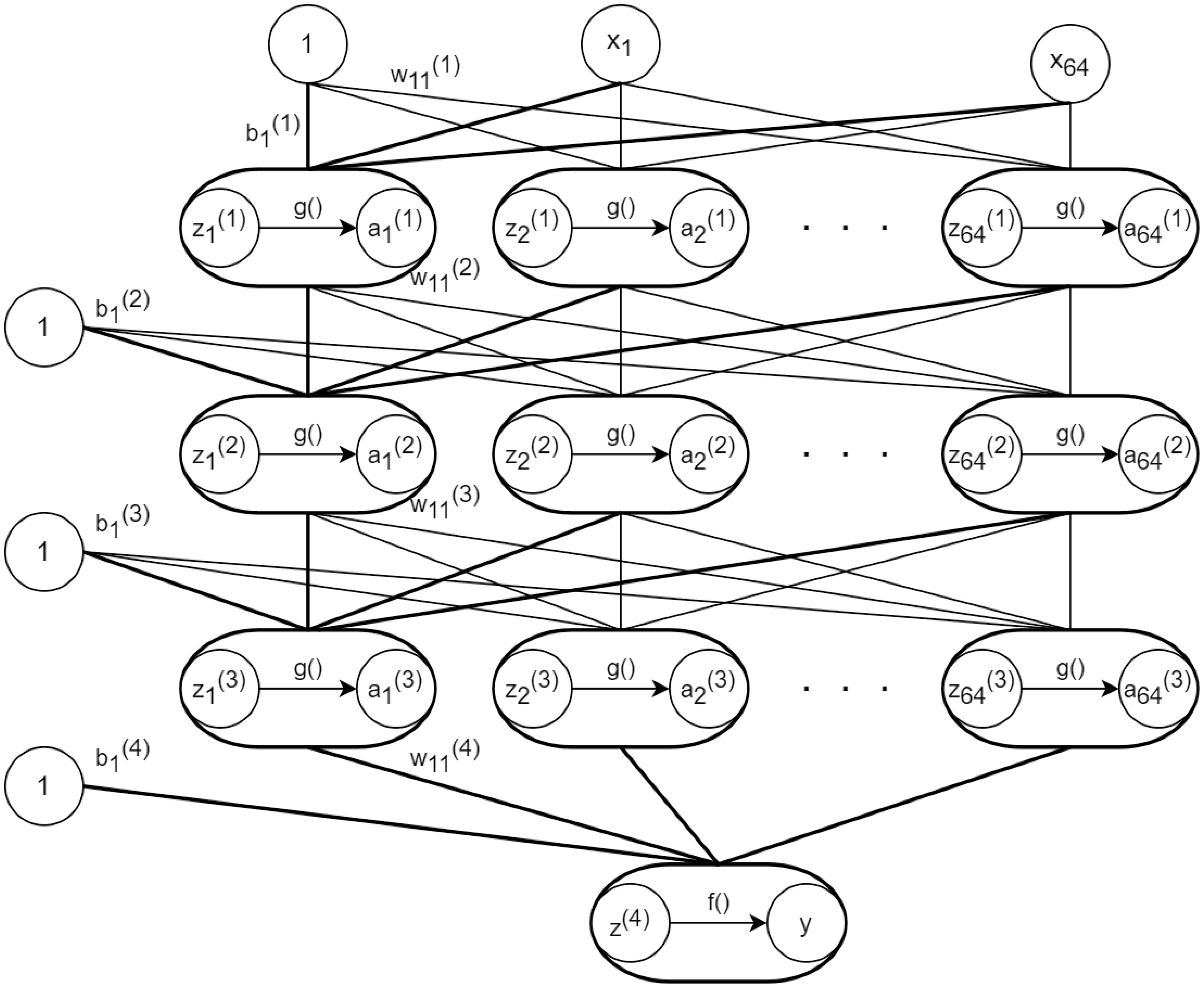
Figure 1 The specific structure of DNN.

2.2 Catboost regression

CatBoost regression is a machine learning algorithm based on Gradient Boosting Decision Tree. It utilizes the gradient boosting algorithm to train the model with the objective of minimizing the loss function and achieving better performance in classification and regression tasks. Compared to traditional gradient boosting decision tree algorithms, CatBoost regression not only possesses high accuracy in predicting feature importance but also distinguishes the relative contributions of different features to the dependent variable.

The relative contribution of a specific feature in a single decision tree is measured by equation (4), where $M$ represents the number of iterations and $J_j^2$ denotes the relative contribution value of feature $j$ . The calculation method for $J_J^2(T)$ is shown in equation (5), where $L-1$ indicates the number of non-leaf nodes in the tree, $v_t$ corresponds to the feature associated with node t, and $i_t^2$ represents the decrease in squared loss after the split at node $t$. A higher reduction in $i_t^2$ signifies a greater relative contribution of the feature to its corresponding node (SPSSRRO).

$\begin{array}{ll}{J}_j^2=\frac{1}{M{\sum }_{m=1}^M{J}_J^2(T_m)}& (4)\end{array}$

$\begin{array}{ll}{J}_J^2(T)={\displaystyle \sum _{t=1}^{L-1}}{i}_t^{2}I({\upsilon }_t=J)& (5)\end{array}$

2.3 RANSAC regression

The foundation of RANSAC lies in the residuals and variance in least squares regression. In least squares regression, a regression model is fitted by minimizing the sum of squared residuals. However, in RANSAC regression, as outliers may exist in the data, directly minimizing the sum of squared residuals may lead to biased fits. Therefore, an iterative weighted least squares estimation of regression coefficients is employed.

RANSAC works by randomly sampling the dataset and selecting inliers (data points that fit well) and outliers. Then, another round of least squares regression is performed using only the inliers, resulting in a regression model as shown in equation (6). In this equation, ${\beta }_1,{\beta }_2,···,{\beta }_p$ represent the unknown regression coefficients, $e_1,e_2,···,e_p$ are independently and identically distributed with a mean of 0. The weights for each data point are determined based on the residuals, where data points with larger residuals are assigned smaller weights to reduce the influence of outliers, and data points with larger residuals are assigned larger weights. This process is iterated multiple times to achieve robustness.

$\begin{array}{ll}{Y}_i={\displaystyle \sum _{j=1}^P}{x}_{ij}{\beta }_j+e_{i}i=1,2,n& (6)\end{array}$

3 Influencing factors identification

3.1 Influencing factors identify

(Zhao et al., 2022) analyzed the impact of BDI, CCBFI, and container throughput on the container market using an autoregressive integrated moving average model and exponential smoothing model. (Hsiao et al., 2014) investigated the lead-lag relationship between BDI and CCFI through cointegration analysis and the Granger causality test. (Tsioumas and Papadimitriou, 2018) explored the influence of coal on maritime trade using cointegration analysis, the Granger causality test, and impulse response analysis. Zheng and Yang ()zheng2016hub discussed the economies of scale in Yangtze River container shipping. Additionally, an increase in aluminum prices may raise production costs in related industries, thereby affecting shipping demand and container freight rates, potentially leading to fluctuations in CCFI. Based on previous literature and the actual situation, this study selected the following six factors for quantitative analysis of their impact on CCFI.

3.1.1 China Coastal Bulk Freight Index

China is one of the world’s largest producers and exporters of goods, making its freight demand and freight rate levels crucial to the global shipping market. The China Coastal Bulk Freight Index (CCBFI) serves as a barometer for China’s major coastal ports’ bulk freight rates. It timely reflects changes in freight transport and aids the Chinese government in macroeconomic regulation of the coastal shipping market, fostering the healthy development of China’s coastal shipping market. Additionally, CCBFI also reflects the conditions of the Chinese container shipping market. Although bulk cargo and container transport are distinct markets, they are both integral components of the maritime industry. Therefore, fluctuations in the five commodity components (coal, grain, metal ore, refined oil, and crude oil) included in the CCBFI can impact changes in the China Container Freight Index (CCFI).

3.1.2 Baltic Dry Index

The BDI reflects the supply and demand relationship and price trends in the international dry bulk market. It is calculated based on the weighted average of spot rates from several major shipping routes worldwide and is published by the Baltic Exchange. The BDI is widely regarded as the “barometer” of dry bulk shipping and has long been used as one of the most important indicators for measuring shipping costs. In recent years, it has also become an important indicator for global trade and the economy. As the dry bulk market and the container market both belong to the shipping industry, they can also have an impact on the China Container Freight Index (CCFI).

3.1.3 Yangtze River Container Freight Index

The Yangtze River Container Freight Index reflects the changes in container freight rates along the Yangtze River, and it is calculated based on actual shipping data from major ports and routes along the Yangtze River. It is published by the Chinese Shipping Information Network. The Yangtze River Container Freight Index is an important indicator of the inland container shipping market along the Yangtze River, while the CCFI reflects the overall price changes in the container shipping market in China. As the Yangtze River serves as a major transportation artery in China’s inland region, the price fluctuations in the inland container shipping market along the Yangtze River can have an impact on the overall market, that is, the price level of CCFI.

3.1.4 Global: Aluminum (minimum purity of 99.5%, London Metal Exchange spot price): UK landed price

This index represents the onshore price of aluminum spot trading on the London Metal Exchange in the United Kingdom, which reflects the price trends and levels in the global aluminum market. Firstly, aluminum is one of the most abundant metallic elements on Earth and is a vital industrial raw material globally. It has extensive applications in sectors such as construction, transportation, power transmission, electronics, and packaging (Li et al., 2020). Therefore, changes in aluminum prices can affect the production costs and product prices in related industries, consequently influencing their transportation demand. Secondly, aluminum prices are influenced by various macroeconomic factors, including global economic conditions, supply and demand balance, trade policies, and exchange rate fluctuations. These factors indirectly impact the demand and prices in the shipping market as well. Hence, aluminum trade and prices also have implications for the development of the shipping market. For instance, an increase in the transportation demand for aluminum products can contribute to the prosperity of the shipping market.

3.1.5 Major ports: container throughput

Major ports refer to ports that have reached or exceeded a certain scale of cargo throughput annually, while container throughput refers to the number of containers handled by a port within a year (Xiao et al., 2023), including container loading and unloading. Container throughput is one of the key factors determining the influence of a port. It plays an important role in domestic cargo exchange and foreign trade transportation and serves as a crucial measurement standard for global trade (Loske, 2020). It can directly reflect the development trends of ports (Huang et al., 2015). Therefore, as an important indicator of container development, port container throughput can provide a fundamental basis for studying the trends of the CCFI.

3.1.6 Coal price: US Central Appalachia: coal spot price index

This index is used to reflect the spot price of coal in the Appalachian region of the American Midwest. It can also serve as a reference indicator for the overall price trend of the coal market and have a certain impact on the price fluctuations in the global coal market. Fossil fuel trade(including coal, crude oil, and natural gas), accounts for over 80% of global primary energy consumption (Wang et al., 2022), with coal being a major contributor (Sahu et al., 2014) and playing a significant role in global trade (Wang et al., 2022; Xiao and Cui, 2023). Therefore, changes in the supply and demand dynamics and price fluctuations in the global coal market may affect international trade and the shipping market. On the other hand, as an important indicator that objectively reflects the global container market conditions, the CCFI has become the world’s second-largest freight index (Hsiao et al., 2014). Its price level and market supply-demand dynamics may be influenced by various factors such as the global economic and trade environment(Lu et al., 2023) and the competitive landscape of the shipping market, which can also impact the supply and demand dynamics and price fluctuations in the coal market. Therefore, this study selects a comprehensive index calculated from the spot price of coal in the Appalachian region of the American Midwest as one of the influencing factors of the CCFI for research purposes.

3.2 Data collection and processing

In this study, data for “CCFI”, “CCBFI”, “BDI”, “Yangtze River Container Freight Index”, “Global: Aluminum (minimum purity of 99.5%, LME spot price): UK landed price”, “Major Ports: Container Throughput” and “Coal Price: Appalachian region of the United States: Coal spot price index” were sourced from the Tonghuashun iFinD platform. Among these, “Major Ports: Container Throughput” had a small number of missing values, which were supplemented by taking the average of the data from the preceding and following months.

As “BDI” is daily data, “CCFI” and “CCBFI” are weekly data, “Yangtze River Container Freight Index” is monthly data, and “Global: Aluminum (minimum purity of 99.5%, LME spot price): UK landed price” and “Coal Price: Appalachian region of the United States: Coal spot price index” are annual data. To make the data consistent in frequency, all the data were aggregated to monthly units. The annual data for “Global: Aluminum (minimum purity of 99.5%, LME spot price): UK landed price” and “Coal Price: Appalachian region of the United States: Coal spot price index” were converted to monthly data, while the remaining data were averaged for the corresponding month. The sample period covers January 2008 to December 2022.

3.3 Descriptive statistical analysis

According to the table, a total of 180 data observations are available for “CCFI,” “CCBFI,” “BDI,” “Yangtze River Container Freight Index,” “Global: Aluminum (minimum purity 99.5%, LME spot price): UK spot price,” “Major Ports: Container Throughput,” and”Coal Price: US Central Appalachia: Coal Spot Price Index.” The table shows the maximum value, minimum value, average value, standard deviation, and median for each of these variables. Table 1 displays the data statistical analysis for each indicator. For “CCFI,” the kurtosis is 4.66, which is greater than 3, indicating a heavy-tailed distribution. The skewness is 2.39, which is greater than 0, indicating a right-skewed distribution. For “CCBFI,” the kurtosis is 7.00, which is greater than 3, indicating a heavy-tailed distribution. The skewness is 2.37, which is greater than 0, indicating a right-skewed distribution. For “BDI,” the kurtosis is 10.60, which is greater than 3, indicating a heavy-tailed distribution. The skewness is 3.04, which is greater than 0, indicating a right-skewed distribution. For the “Yangtze River Container Freight Index,” the kurtosis is 1.36, which is less than 3, indicating a thin-tailed distribution. The skewness is 1.23, which is greater than 0, indicating a right-skewed distribution. For “Global: Aluminum (minimum purity 99.5%, LME spot price): UK spot price,” the kurtosis is 0.03, which is less than 3, indicating a thin-tailed distribution. The skewness is 1.23, which is greater than 0, indicating a right-skewed distribution. For “Major Ports: Container Throughput,” the kurtosis is -1.05, which is less than 3, indicating a thin-tailed distribution. The skewness is 0.01, which is greater than 0, indicating a right-skewed distribution. For “Coal Price: US Central Appalachia: Coal Spot Price Index,” the kurtosis is 0.83, which is less than 3, indicating a thin-tailed distribution. The skewness is 1.16, which is greater than 0, indicating a right-skewed distribution. The comparison of kurtosis and skewness for the7 variables is shown in Figure 2.

TABLE 1

Table 1 Results of descriptive statistical analysis of the data.

FIGURE 2

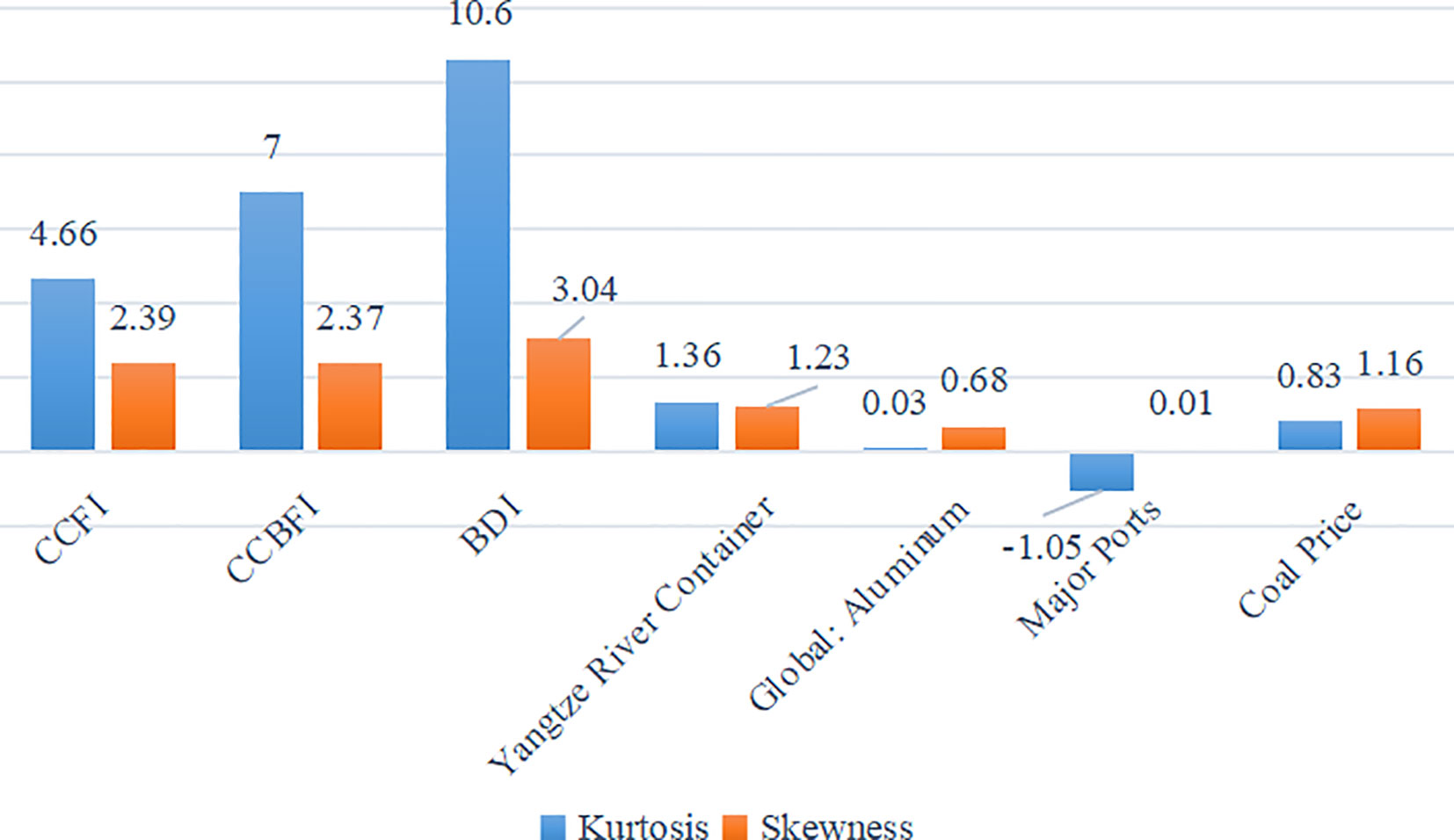
Figure 2 Kurtosis and skewness histograms of the data.

4 Experimental results

4.1 DNN

Based on the collected monthly data of CCFI and its six influencing attributes from January 2008 to December 2022, a total of 180 data points are available. The dataset is divided into a training set consisting of 125 data points and a test set consisting of 2 data points. The training process involves training a model using the training set. The model is then used to predict the CCFI values for the test set, and the accuracy of the model is evaluated based on the actual values of the test set. The training cycle is set to 50, and the mean squared error (MSE) is used as the loss function, while the mean absolute error (MAE) is used as the performance metric. The RMSProp optimization algorithm is utilized. K-fold cross-validation is employed as a common method for evaluating model performance in deep learning. It provides a more reliable estimate of the model’s generalization ability by dividing the dataset into K subsets, using one subset as the validation set, and the remaining K-1 subsets as the training set. This process is repeated K times, and the average results are taken to reduce bias caused by different choices of training and validation sets, thus providing a more reliable evaluation of the model’s performance. Since the training set data is limited, K-fold cross-validation is used. In this case, K is set to 4, indicating that the training set is divided into four parts for cross-validation. Each time, one part is used as the validation set, while the remaining three parts are used as the training set. The line graph illustrating the relationship between training cycles and MAE is shown in Figure 3.

FIGURE 3

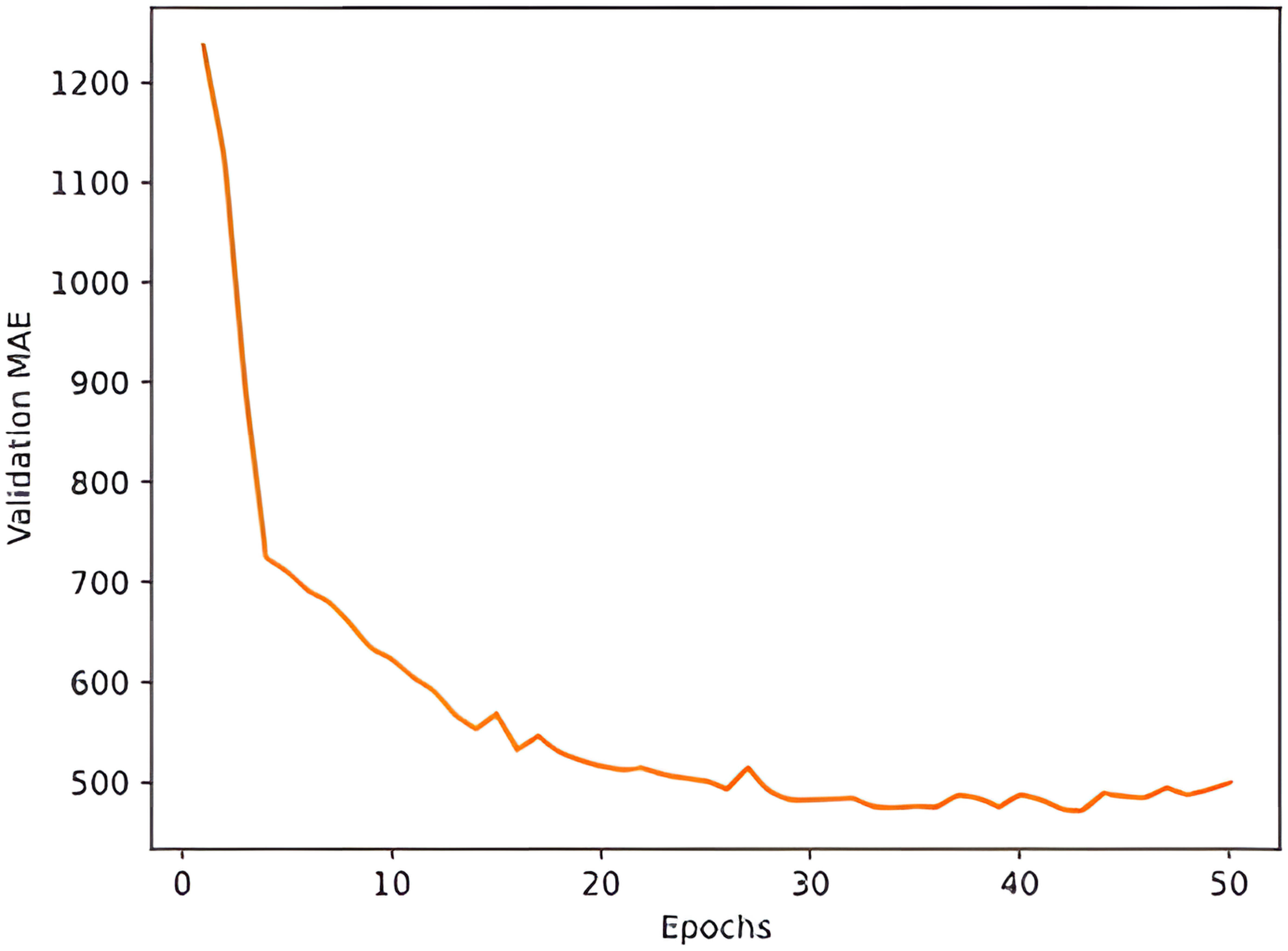
Figure 3 Line graph of the relationship between training cycles and MAE.

As shown in Table 2, lists the model evaluation results for the six attributes influencing CCFI and the prediction of CCFI using DNN from 2008 to 2022. A higher $R^2$ value indicates better performance. The MSE value is 35237.797 in the test set and 11100.341 in the training set. The RMSE value is 187.717 in the test set and 105.358 in the training set. The MAE value is 157.457 in the test set and 93.591 in the training set. The MAPE value is 0.199 in the test set and 3.233 in the training set. The $R^2$ value is 0.272 in the test set and 0.882 in the training set.

TABLE 2

Table 2 DNN evaluation results.

4.2 Catboost regression

This chapter aims to provide a detailed explanation of the modeling details of the CatBoost regression model using the SPSSPRO software. The most important aspect of the modeling process is parameter tuning, which involves adjusting key parameters to avoid over fitting and improve model accuracy. The specific steps for parameter tuning and modeling are as follows:

Step 1, Data Split. In order to evaluate the performance of the model, the dataset is divided into a training set and a test set. Typically, the dataset can be split into a training set of 70% to 80% of the data and the remaining portion as the test set. Since our dataset is relatively small, we will choose to use 80% of the data as the training set and 20% as the test set. Additionally, we will shuffle the data to eliminate any inherent ordering and reduce the model’s dependence on specific orderings, thereby improving the model’s generalization and reliability.

Step 2, Parameter Tuning. The key parameters to determine in the CatBoost regression model are: iterations, learning-rate, depth, and regularization. For the iteration count, it represents the number of training rounds for the model. A larger iteration count can increase the training time but may improve the model’s performance to some extent. The learning rate controls the step size at which the model updates the weights during each iteration. A higher learning rate can accelerate the convergence of the model but may lead to over fitting. On the other hand, a lower learning rate can improve the stability and generalization ability of the model but may result in longer training time. In the statement you provided, it mentions that setting the learning rate to 0.1 is generally appropriate. However, considering the complexity of the experiment, you chose to evaluate several reasonable ranges of values. With the other parameters set to their initial values, you tested different learning rates, such as iterations=[50, 100, 150, 200], and evaluated their performance on the validation set. Finally, we selected 100 iterations as the optimal number of iterations based on the evaluation results. The depth of the tree determines the complexity of the model. Deeper trees can capture more feature interactions, but they can also lead to over fitting. Shallower trees may not be able to fully capture the complexity of the data. Based on the adjusted number of iterations and learning rate, we conducted experiments with depth=[8, 9, 10, 11]. It was found that the model achieved the highest accuracy when the depth was set to 10. The regularization parameter helps prevent model over fitting. In CatBoost, the regularization parameters mainly include L1 regularization and L2 regularization. We used L2 regularization and set the regularization parameter values to [0.01, 0.1, 1.0]. Finally, we determined the regularization parameter value to be 1.0.

Finally, using the parameter tuning results mentioned earlier, we apply them to the data for modeling. Table 3 presents the important proportions of the six selected features for CCFI.

TABLE 3

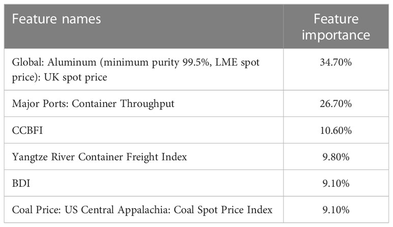
Table 3 Feature importance.

The prediction results of CatBoost regression are shown in Table 4. We can see that the mean squared error (MSE) and mean absolute error (MAE) of the training set, which represent the expected value of the squared difference between the predicted values and the actual values, are both small. Additionally, the $R^2$ value of 1 indicates a high accuracy of the model. Moreover, the $R^2$ value of 0.875 for the test set indicates good performance.

TABLE 4

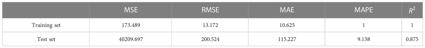
Table 4 Evaluation results of the CatBoost regression model.

The goodness of fit plot for the CatBoost regression model is shown in Figure 4. The blue line represents the true values of the test set, while the green line represents the predicted values of the test set. The two lines overlap to a great extent. From the Figure, it can be observed that after training, an ideal CatBoost regression model has been obtained.

FIGURE 4

Figure 4 CatBoost regression model prediction results.

4.3 Robust regression

A robust regression model is constructed with CCFI as the dependent variable and “CCBFI,” “BDI,” “Yangtze River Container Freight Index,” “Global: Aluminum (minimum purity 99.5%, LME spot price): UK landed price,” “Ports: Container Throughput of Major Ports,” and “Coal Price: US Central Appalachian: Coal Spot Price Index” as independent variables. Let CCFI be Y, and let “CCBFI,” “BDI,” “Yangtze River Container Freight Index,” “Global: Aluminum (minimum purity 99.5%, LME spot price): UK landed price,” “Ports: Container Throughput of Major Ports,” and “Coal Price: US Central Appalachian: Coal Spot Price Index” be $X_1,X_2,X_3,X_4,X_5,X_6$ respectively.

Thus, a multiple linear regression model can be established as shown in equation (7)

$\begin{array}{ll}Y=C_0+C_1\times X_1+C_2\times X_2+C_3\times X_3+C_4\times X_4+C_5\times X_5+C_6\times X_6& (7)\end{array}$

Where $C_0$is the constant term, and $C_1,C_2,C_3,C_4,C_5,C_6$ are the coefficients of each variable. The regression results are shown in the Table 5.

TABLE 5

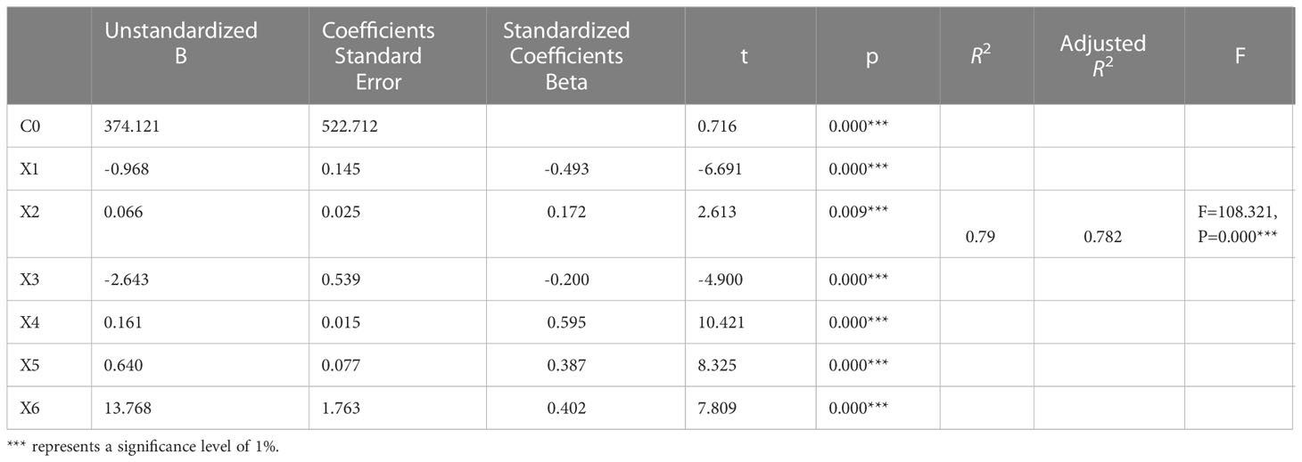
Table 5 Robust regression result.

The regression equation is shown in equation (8) (using non-standardized coefficients).

$\begin{array}{ll}Y=374.121-0.968\times X_1+0.066\times X_2+2.643\times X_3+0.161\times X_4+0.64\times X_5+13.768\times X_6& (8)\end{array}$

The regression model has an $R^2$ value of 0.79, indicating that 79% of the variation in Y can be explained by the model, indicating a good fit. By observing the regression model, it can be noted that CCFI is positively correlated with “BDI”, “Global: Aluminum (minimum purity of 99.5%, LME spot price): UK landed price”, “Major Ports: Container Throughput”, and “Coal Price: US Central Appalachian: Coal spot price index”, while CCFI is negatively correlated with “CCBFI” and “Yangtze River Container Freight Index”.

Performing an F-test to test the overall significance of the regression equation.

The null hypothesis($H_0$) is stated as follows: $C_1=C_2=C_3=C_4=C_5=C_6=0$The alternative hypothesis($H_1$) is stated as follows: at least one of the coefficients $C_1,C_2,C_3,C_4,C_5,C_6$ is not equal to zero.

As shown in the Table 5, $P=0$. Therefore, we reject the null hypothesis, indicating that there is a linear relationship between $Y$ and $X_1,X_2,X_3,X_4,X_5,X_6$.

Based on the results of the robust regression model, the variable “Global: Aluminum (minimum purity 99.5%, LME spot price): UK delivered price” was found to have the most significant impact on the CCFI. Aluminum is one of the most widely used important metals globally. It possesses characteristics such as lightweight, good conductivity, and corrosion resistance, making it widely applied in various industries including aerospace, automotive, construction, packaging, and more.

From the perspective of raw material costs, global aluminum production ranks third after iron and copper, and it requires a significant amount of raw materials like bauxite. However, the distribution of global bauxite reserves is uneven, and international trade of bauxite requires shipping. If global aluminum ore prices rise, both production and transportation costs of aluminum may increase, thus impacting the shipping market.

Considering international trade and shipping demand, aluminum is a widely traded commodity across various industries, including construction, automotive manufacturing, aerospace, and shipbuilding. Aluminum plays a crucial role in the shipbuilding industry due to its lightweight and excellent corrosion resistance. It finds applications in ship structures, equipment, and interior components.

From the perspective of supply and demand in the metal market, the demand for aluminum in various industries fluctuates with macroeconomic conditions, geopolitical factors, and trade policies. Additionally, changes in aluminum smelting capacity, utilization rates, and energy costs also affect the supply and demand dynamics of aluminum. Therefore, fluctuations in aluminum demand and supply indirectly influence the CCFI through changes in shipping demand, leading to fluctuations in the index.

In conclusion, changes in aluminum prices have a significant impact on the fluctuations of the CCFI.

4.4 Comparison of results

In this study, we employed DNN (Deep Neural Network), CatBoost regression model, and Robust regression model to analyze and predict the impact of “CCBFI”, “BDI”, “Yangtze River Container Freight Index”, “Global: Aluminum (minimum purity of 99.5%, LME spot price): UK landed price”, “Major Ports: Container Throughput”, and “Coal Price: US Central Appalachian Coal Spot Price Index” on CCFI. Our objective was to identify the most effective model for predicting CCFI and compare the performance of these models.

When presenting the experimental results, we selected MSE, RMSE, MAE, MAPE, and $R^2$ as commonly used metrics for evaluating model performance and accuracy. MSE measures the average of the squared differences between predicted values and true values. RMSE is the square root of MSE and has the same unit as the original data, making it more intuitively understandable. MAE measures the average of the absolute differences between predicted values and true values. MAPE measures the average of the percentage differences between predicted values and true values. Smaller values for these four metrics indicate smaller percentage differences between the model’s predictions and the true values. $R^2$ measures the proportion of the variance in the dependent variable that can be explained by the regression model. $R^2$ values range from 0 to 1, where values closer to 1 indicate better ability of the model to explain the variance in the dependent variable and better predictive performance, while values closer to 0 indicate poorer explanatory power and poorer predictive performance. These metrics reflect the performance and accuracy of the model. Smaller values of MSE, RMSE, MAE, and MAPE, as well as larger values of $R^2$, indicate smaller differences between the model’s predictions and the true values, indicating better model performance and higher accuracy. These metrics can be used for comparing the performance of different models, selecting the best model, tuning model parameters, and evaluating the model’s generalization ability on new data.

Based on the analysis of the experimental results using $R^2$ , we draw the following conclusions: The DNN model exhibits the best predictive performance, with an $R^2$ of 0.882. The CatBoost regression model achieves an $R^2$ of 0.875 on the test set, while the Robust regression model has an $R^2$ of 0.79. This indicates that DNN possesses strong learning ability and nonlinear fitting capability, allowing it to capture the complex relationship between input features and the target variable more effectively. It is suitable for handling large-scale data and high-dimensional features, automatically extracting features, and conducting efficient pattern recognition. Therefore, the DNN model can accurately predict the variations in CCFI and provide higher prediction accuracy.

Based on the analysis of the time and space complexity of the three models, the DNN model usually has a higher time complexity, which depends on the number of layers, the number of neurons in each layer, and the number of training iterations. It can be approximated as O($E\ast n\ast m$), where E is the number of training iterations (100), n is the sample size (180), and m is the number of model parameters ($64\ast (64+1)$). The CatBoost model has a relatively lower training time complexity due to the efficient optimization strategies and techniques it employs. It can be approximated as O($T\ast n\ast d^2$), where T is the number of iterations (20), n is the sample size (180), and d is the feature dimension (7).The time complexity of the robust regression model is comparable to that of ordinary least squares regression, which is approximately O($n^3$), where n is the sample size (180).The space complexity of the DNN model includes storing the training data and model parameters. The space required for storing the training data is proportional to the size of the dataset, i.e., O($n\ast d$), where n is the sample size and d is the feature dimension. Additionally, the DNN model needs to store the weights and biases of each neuron, so the space complexity of the model parameters is dependent on the model’s scale. The space complexity of the CatBoost model mainly consists of storing the training data and model parameters. The space required for storing the training data is proportional to the size of the dataset, i.e., O($n\ast d$), where n is the sample size and d is the feature dimension. Additionally, CatBoost needs to store the parameters and split points of each decision tree, so the space complexity of the model parameters is related to the number and depth of the trees. The space complexity of the robust regression model mainly includes storing a copy of the original dataset and the model parameters. The space required for storing the dataset is proportional to the size of the dataset, i.e., O(n), where n is the sample size (180). Additionally, the robust regression model needs to store the iterative computation results for each sample, so the space complexity of the model parameters is related to the size of the dataset.

In summary, based on our research findings, the DNN model performs the best in analysis and prediction, followed by the CatBoost regression model in second place, and the Robust regression model in third place. These conclusions provide valuable guidance for selecting the appropriate model for analyzing and predicting CCFI. They also offer important insights into model performance and application scenarios. However, choosing the right model should also consider the specific problem and data characteristics, and adjustments and optimizations should be made according to the requirements of practical applications.

5 Conclusions and suggestions

According to our research findings, the DNN model exhibits the best performance in analysis and prediction, followed by the CatBoost regression model in second place, and the Robust regression model in third place. The Robust regression model is characterized by its relatively simple principles, making it easy to comprehend and implement, suitable for analyzing simple linear relationships. In contrast, the DNN and CatBoost regression models are more complex, requiring deeper theoretical and technical knowledge, as well as more extensive model tuning and training time, especially when dealing with large-scale data and complex features. The Robust regression model, on the other hand, requires less training time and computational resource consumption, making it suitable for quick analysis and prediction.

Therefore, we suggested that, depending on the company’s capabilities, different models should be chosen for predicting CCFI. For companies with greater resources, the DNN and CatBoost regression models are more suitable. These companies typically operate in more complex business environments with larger data volumes, and these models can effectively handle large-scale data and capture complex relationships, providing more accurate predictions and decision support. For companies with limited resources, the Robust regression model is more practical. Given their smaller business scales and limited data compared to larger companies, the Robust regression model can still offer reliable analysis results while saving time and resource costs.

For small-scale companies, the Robust regression model offers efficiency in terms of time and resource consumption. Robust regression is a powerful statistical method that can provide reliable analysis results even in the presence of outliers or anomalies in the data. In terms of time, the Robust regression model is typically faster than complex nonlinear models or machine learning methods. Its computational complexity is relatively low, allowing for faster results when dealing with large-scale datasets. This means that small-scale companies can perform data analysis and make decisions more quickly without requiring excessive time and computational resources. However, the Robust regression model also has its limitations. Firstly, it assumes that the error term in the data follows a certain distribution, often assuming a normal distribution. If the error term in the data does not adhere to these assumptions, the effectiveness of the Robust regression model may decrease. Therefore, when selecting a model, small-scale companies need to consider the characteristics of their data and the objectives of their analysis. If the dataset exhibits nonlinear relationships or particularly complex structures, or if there are a significant number of outliers in the data, the Robust regression model may not be the best choice. In such cases, they may need to consider other models that are more suitable for handling these features.

In conclusion, the DNN, CatBoost regression model, and Robust regression model possess distinct characteristics in analyzing and predicting CCFI. The choice of an appropriate model should consider the company’s scale and requirements. However, specific problems and data features should also be taken into account, and the selected model should be adjusted and optimized to suit practical application needs.

While this study has yielded valuable research findings, it is important to acknowledge its limitations. For instance, the data sources used in this study may have inherent uncertainties and biases during the data processing stage. Additionally, although multiple factors influencing the shipping market were investigated, there may be other potentially significant factors that were not considered. In future research, expanding the selection of variables can lead to more comprehensive analysis results. Moreover, while DNN, CatBoost regression, and Robust regression models were chosen as the analysis and prediction framework in this study, other machine learning or statistical models may also hold potential. Further exploration of the applicability and performance comparison of different models can be pursued in future work to identify optimal predictive models. To further advance the understanding and impact of our research, several avenues for future work emerge: Data Updates and Expansion: The shipping market is a dynamic system, necessitating regular updates and expansion of the dataset to reflect the latest market changes. Future research can collect more data, including additional factors and longer time spans, to improve the accuracy and stability of prediction models. Model Improvements and Optimization: Further enhancing and optimizing the adopted models to enhance their predictive performance and robustness. For example, different model architectures, hyperparameter tuning, and feature engineering techniques can be explored to optimize model performance. Consideration of Additional Factors and Complex Relationships: The shipping market is influenced by multiple factors with complex interrelationships. Future research can explore additional factors and their intricate relationships, such as market competition strategies, policy changes, and global economic dynamics, to provide a more comprehensive analysis and prediction of the shipping market.

Data availability statement

The original contributions presented in the study are included in the article/Supplementary Material. Further inquiries can be directed to the corresponding author.

Author contributions

XT, YY, and YL contributed to conception and design of the study. XT collected and processed the original data. XT, YY, and SM used the three models to analyze the data. XT wrote the first draft of the manuscript. XT, YY, and YL wrote sections of the manuscript. All authors contributed to the article and approved the submitted version.

Conflict of interest

The authors declare that the research was conducted in the absence of any commercial or financial relationships that could be construed as a potential conflict of interest.

Publisher’s note

All claims expressed in this article are solely those of the authors and do not necessarily represent those of their affiliated organizations, or those of the publisher, the editors and the reviewers. Any product that may be evaluated in this article, or claim that may be made by its manufacturer, is not guaranteed or endorsed by the publisher.

Supplementary material

The Supplementary Material for this article can be found online at: https://www.frontiersin.org/articles/10.3389/fmars.2023.1245542/full#supplementary-material

References

Chen Y., Liu B., Wang T. (2021). Analysing and forecasting China containerized freight index with a hybrid decomposition–ensemble method based on emd, grey wave and arma. Grey Systems: Theory Appl. 11, 358–371. doi: 10.1108/GS-05-2020-0069

CrossRef Full Text | Google Scholar

Hancock J. T., Khoshgoftaar T. M. (2020). Catboost for big data: an interdisciplinary review. J. big Data 7, 1–45. doi: 10.1186/s40537-020-00369-8

CrossRef Full Text | Google Scholar

Hsiao Y.-J., Chou H.-C., Wu C.-C. (2014). Return lead–lag and volatility transmission in shipping freight markets. Maritime Policy Manage. 41, 697–714. doi: 10.1080/03088839.2013.865849

CrossRef Full Text | Google Scholar

Huang A., Lai K. K., Qiao H., Wang S., Zhang Z. (2015). An interval knowledge based forecasting paradigm for container throughput prediction. Proc. Comput. Sci. 55, 1381–1389. doi: 10.1016/j.procs.2015.07.126

CrossRef Full Text | Google Scholar

Huang G., Wu L., Ma X., Zhang W., Fan J., Yu X., et al. (2019). Evaluation of catboost method for prediction of reference evapotranspiration in humid regions. J. Hydrology 574, 1029–1041. doi: 10.1016/j.jhydrol.2019.04.085

CrossRef Full Text | Google Scholar

Jeon J.-W., Duru O., Munim Z. H., Saeed N. (2021). System dynamics in the predictive analytics of container freight rates. Transportation Sci. 55, 946–967. doi: 10.1287/trsc.2021.1046

CrossRef Full Text | Google Scholar

Khaki S., Wang L. (2019). Crop yield prediction using deep neural networks. Front. Plant Sci. 10, 621. doi: 10.3389/fpls.2019.00621

PubMed Abstract | CrossRef Full Text | Google Scholar

LeCun Y., Bengio Y., Hinton G. (2015). Deep learning. nature 521, 436–444. doi: 10.1038/nature14539

PubMed Abstract | CrossRef Full Text | Google Scholar

Li Y., Yue Q., He J., Zhao F., Wang H. (2020). When will the arrival of China’s secondary aluminum era? Resour. Policy 65, 101573. doi: 10.1016/j.resourpol.2019.101573

CrossRef Full Text | Google Scholar

Loske D. (2020). The impact of covid-19 on transport volume and freight capacity dynamics: An empirical analysis in German food retail logistics. Transportation Res. Interdiscip. Perspect. 6, 100165. doi: 10.1016/j.trip.2020.100165

CrossRef Full Text | Google Scholar

Lu J., Wu X., Wu Y. (2023). The construction and application of dual-objective optimal speed model of liners in a changing climate: taking yang ming route as an example. J. Mar. Sci. Eng. 11, 157. doi: 10.3390/jmse11010157

CrossRef Full Text | Google Scholar

Ma Y., Jiang Q. (2018). A robust and high-precision automatic reading algorithm of pointer meters based on machine vision. Measurement Sci. Technol. 30, 015401. doi: 10.1088/1361-6501/aaed0a

CrossRef Full Text | Google Scholar

Ni K., Jin H., Dellaert F. (2009). GroupSAC: Efficient consensus in the presence of groupings, IEEE 12th International Conference on Computer Vision. 2193–2200. doi: 10.1109/ICCV.2009.5459241

CrossRef Full Text | Google Scholar

Olofsson K., Holmgren J., Olsson H. (2014). Tree stem and height measurements using terrestrial laser scanning and the ransac algorithm. Remote Sens. 6, 4323–4344. doi: 10.3390/rs6054323

CrossRef Full Text | Google Scholar

Sahu S. G., Chakraborty N., Sarkar P. (2014). Coal–biomass co-combustion: An overview. Renewable Sustain. Energy Rev. 39, 575–586. doi: 10.1016/j.rser.2014.07.106

CrossRef Full Text | Google Scholar

Tsioumas V., Papadimitriou S. (2018). The dynamic relationship between freight markets and commodity prices revealed. Maritime Economics Logistics 20, 267–279. doi: 10.1057/s41278-016-0005-0

CrossRef Full Text | Google Scholar

Wang W., Fan L., Zhou P. (2022). Evolution of global fossil fuel trade dependencies. Energy 238, 121924. doi: 10.1016/j.energy.2021.121924

CrossRef Full Text | Google Scholar

Xiao G., Cui W. (2023). Evolutionary game between government and shipping enterprises based on shipping cycle and carbon quota. Front. Mar. Sci. 10, 1132174. doi: 10.3389/fmars.2023.1132174

CrossRef Full Text | Google Scholar

Xiao G., Wang T., Luo Y., Yang D. (2023). Analysis of port pollutant emission characteristics in united states based on multiscale geographically weighted regression. Front. Mar. Sci. 10, 1131948. doi: 10.3389/fmars.2023.1131948

CrossRef Full Text | Google Scholar

Xu L., Zou Z., Zhou S. (2022). The influence of covid-19 epidemic on bdi volatility: An evidence from garch-midas model. Ocean Coast. Manage. 229, 106330. doi: 10.1016/j.ocecoaman.2022.106330

CrossRef Full Text | Google Scholar

Yin J., Shi J. (2018). Seasonality patterns in the container shipping freight rate market. Maritime Policy Manage. 45, 159–173. doi: 10.1080/03088839.2017.1420260

CrossRef Full Text | Google Scholar

Yu P., Yan X. (2020). Stock price prediction based on deep neural networks. Neural Computing Appl. 32, 1609–1628. doi: 10.1007/s00521-019-04212-x

CrossRef Full Text | Google Scholar

Zhao H.-M., He H.-D., Lu K.-F., Han X.-L., Ding Y., Peng Z.-R. (2022). Measuring the impact of an exogenous factor: An exponential smoothing model of the response of shipping to covid-19. Transport Policy 118, 91–100. doi: 10.1016/j.tranpol.2022.01.015

PubMed Abstract | CrossRef Full Text | Google Scholar

Zhou F., Cui Y., Wang Y., Liu L., Gao H. (2013). Accurate and robust estimation of camera parameters using ransac. Optics Lasers Eng. 51, 197–212. doi: 10.1016/j.optlaseng.2012.10.012

CrossRef Full Text | Google Scholar

Zhou F., Pan H., Gao Z., Huang X., Qian G., Zhu Y., et al. (2021). Fire prediction based on catboost algorithm. Math. Problems Eng. 2021, 1–9. doi: 10.1155/2021/1929137

CrossRef Full Text | Google Scholar

Zhu F., Li X., Mcgonigle D., Tang H., He Z., Zhang C., et al. (2019). Analyze informant-based questionnaire for the early diagnosis of senile dementia using deep learning. IEEE J. Trans. Eng. Health Med. 8, 1–6. doi: 10.1109/JTEHM.2019.2959331

CrossRef Full Text | Google Scholar