A SST-constructed Ocean Heat Content index in crossing ENSO spring persistence barrier

1 Introduction

El Niño-Southern Oscillation (ENSO) is the most significant interannual signal on earth, which impacts global climate, extreme weather, and the environment through teleconnection (McPhaden et al., 2006). Therefore, forecasting ENSO events has garnered great attention for decades (Balmaseda et al., 1995; Barnston et al., 2012). One striking feature in ENSO prediction studies is the spring persistence barrier (SPB) or associated spring predictability barrier (Torrence and Webster, 1998; Ren et al., 2016). This SPB can be mainly noticed in the observation of tropical Pacific sea surface temperature (SST) anomalies variability (e.g., Niño3.4; 5°S-5°N, 170°W-120°W; blue box in Figure 1). It shows that ENSO predictability, as estimated by the autocorrelation function (ACF) of SST anomaly, tends to drop substantially during the boreal spring, regardless of different initial months (Liu et al., 2019; Jin et al., 2020).

FIGURE 1

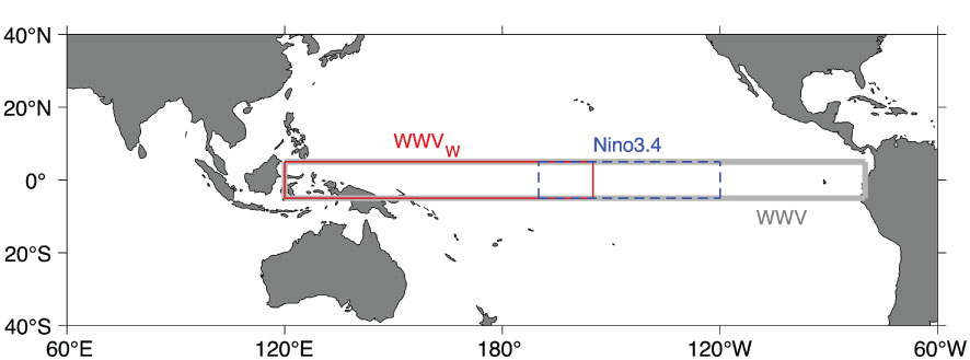
Figure 1 The region of Niño3.4 (5°S~5°N, 170°W~120°W; blue box), WWV (5°S~5°N, 120°E~80°W; gray box) and WWVw (5°S~5°N, 120°E~155°W; red box).

Currently, many studies have proposed various indices to help predict ENSO across SPB. Seleznev and Mukhin (2023) proposed a joint SST-OHC model using Bayesian optimization schemes and revealed a substantial reduction in the seasonal predictability barrier of ENSO and winter barrier for the OHC index. Nigam and Sengupta (2021) proposed an SST index based on regressions of four spatiotemporal modes that better capture ENSO variability and related hydroclimate impact (relative to Nino 3.4 index) at multiple seasonal leads. Planton et al. (2018) proposed the western Pacific OHC as a better predictor of La Niña events. Zhu et al. (2014) in fact proposed that sea surface salinity variability plays an active role in ENSO evolution and is important for forecasting El Niño events. In addition, the Victoria Mode and South Pacific Quadrapole may affect ENSO events approximately 10 months later through the Seasonal Footprint Mechanism or the Trade Wind Charging (Ding et al., 2015; Shi et al., 2022). The warming of the Tropical North Atlantic is believed to stimulate the westward propagation of the equatorial Rossby wave train, which is beneficial for the formation of La Niña after 9 months (Ham et al., 2013). In addition, Chen et al. (2022) found that there is a significant negative correlation between spring SST anomalies in the Tropical Western Atlantic and subsequent winter ENSO variability, which can predict ENSO 10 months in advance. Chen et al. (2020) constructed a multiple linear regression model based on tropical dynamics, ocean-atmosphere feedback, and temperate atmospheric forcing to increase the predictability of ENSO.

Previous studies have shown that the slow evolution of the upper ocean in the tropical Pacific is a major source of predictability for ENSO (Meinen and McPhaden, 2000; Anderson, 2007). Wyrtiki (1985) suggested that accumulated warm water flows eastward in the form of Kelvin waves, leading to the occurrence of El Niño events. According to the recharge oscillator theory of ENSO, Jin (1997) indicated that anomalies in the tropical Pacific Ocean Heat Content (OHC) reach their maximum magnitude before the development of the largest magnitude SST anomalies. Based on that, the index named warm water volume (WWV; 5°S-5°N, 120°E-80°W; gray box in Figure 1; McPhaden, 2003) is widely used in ENSO forecasting, especially for crossing ENSO SPB (Yu and Kao, 2007; Bunge and Clarke, 2014). Recently, the west of warm water volume (WWVw; 5°S-5°N, 120°E-155°W; red box in Figure 1) has been argued to be important for ENSO longer time scale (more than 9 months) forecasting (Izumo et al., 2019).

The lead-lag relationship between OHC and ENSO has not been directly established before 1980 due to the unavailability of reliable subsurface ocean data. Therefore, sea level datasets have been used to investigate the relationship between OHC and ENSO for a longer time range (Wyrtki, 1985). Jin (1997) attempted to demonstrate the effectiveness of the recharge oscillator theory using sea level data. Bunge and Clarke (2014) constructed a sea level-based WWV proxy dating back to 1955 and suggested a small lead time before 1973. However, to the best of our knowledge, no test of this lead-lag relationship has been conducted using SST data.

Reliable SST data has been available since 1950, so we are inspired to explore the lead-lag relationship between OHC and ENSO for a longer time range using an index constructed by SST anomalies. Specifically, according to the recharge oscillator theory, the relationship between SST and OHC anomalies is described (eq. 2.2; Stein et al., 2010; Levine and McPhaden, 2015). According to this relationship, we propose an index (namely SST_H; more details will be described in Section 2.1) to represent OHC as a predictor for ENSO forecasts. This allows us to examine the lead-lag relationship only using SST datasets. Moreover, this index captures the major features of the ocean subsurface, making it effective for crossing ENSO SPB. Compared with WWV (McPhaden, 2012) or WWVw, this is more stable as a predictor on the interdecadal time scale. The method we employ to produce SST_H and the reanalysis data will be presented in Section 2. The comparison between SST_H and WWV/WWVw is shown in Section 3. In Section 4 we will explore the interdecadal change in the lead-lag relationship between SST_H and ENSO SST anomalies. Finally, a summary and discussion will be given in Section 5.

2 Method and data

2.1 An SST-constructed index to represent tropical Pacific Ocean Heat Content

The recharge oscillator model (Jin, 1997) describes the dynamic relationship between the equatorial Pacific thermocline depth (or OHC) anomaly (H) and the eastern SST anomaly (T) and can be written as (Levine and McPhaden, 2015):

$\begin{array}{ll}\frac{dT}{dt}=-\lambda T+{\omega }_{0}H+\sigma \xi & \text{(2.1)}\end{array}$

$\begin{array}{ll}\frac{dH}{dt}=-{\omega }_{0}T& \text{(2.2)}\end{array}$

where λ is the damping rate, ω₀ is the ENSO linear frequency, ξ is white noise (stochastic forcing) and σ is the noise amplitude. Eq. (2.1) indicates the combined effects of the relaxation of SST anomaly (negative feedback), advection, Ekman upwelling, thermocline positive feedback, and noise forcing on the SST anomaly. Eq. (2.2) suggests a description of the basin-wide equatorial oceanic adjustment. Note that the damping term of OHC is neglected here. This is because, on seasonal and longer time scales, changes in OHC are mainly governed by the geostrophic response to the wind stress forcing rather than by the damping itself (Burgers et al., 2005). Here, wind stress can be linearly represented by T and eq. (2.2) is obtained consequently. According to eq. (2.2), there is a phase lag between H and T, suggesting that H can be a predictor for SST at large lead times. Meanwhile, SST can also be a predictor of H changes (see also Figure 2).

FIGURE 2

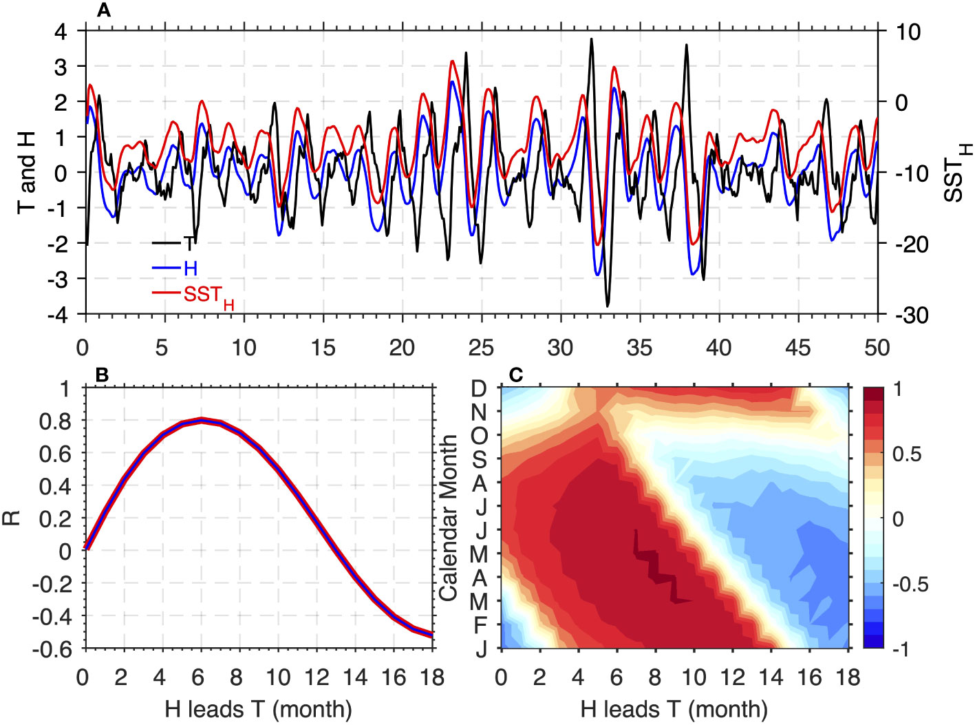
Figure 2 Numerical solution of the recharge oscillation model (eqs.2.1-2.2). $\lambda =0.15*[1 + 1.8sin(\frac{\pi }{6}t)]mont{h}^{-1}$, ${\omega }_0=\frac{2\pi }{30}mont{h}^{-1}$ (A) Time series of T, H and SST_H. (B) The lead-lag cross correlation between T and H (blue line), SST_H (red line). (C) The seasonal cross-correlation of T and H.

Unlike H in eq. (2.2) (WWV or WWV_W), the reliable SST data is longer. This encourages us to construct a new predictor using SST data to represent H. Therefore, mathematically motivated by eq. (2.2) and for prediction purposes, H can be calculated as follows:

$\begin{array}{ll}\text{H}(\text{t})=-{\int }_{t0}^t{\omega }_{0}Tdt\approx -{\omega }_0{\int }_{t0}^{t}Tdt\approx -{\omega }_0({\int }_{t0}^{t-1}Tdt+(T(t)+T(t-1))/2)& \text{(2.3)}\end{array}$

H(t)≈ω₀SST_H(t) and ω₀ does not change dramatically with time compared with SST anomalies, the lead-lag correlation between H and T (r(τ)) can be obtained as follows:

$\begin{array}{ll}\text{r}(\text{τ})=\frac{\langle \text{H}(\text{t}),\text{T }(\text{t})\rangle }{\sqrt{\langle H(t),H(t)\rangle *\langle T(t),T(t)\rangle }}=\frac{{\omega }_0\langle SS{T}_H(t),\text{T }(\text{t})\rangle }{{\omega }_0\sqrt{\langle SS{T}_H(t),SS{T}_H(t)\rangle *\langle T(t),T(t)\rangle }}=\frac{\langle SS{T}_H(t),\text{T }(\text{t})\rangle }{\sqrt{\langle SS{T}_H(t),SS{T}_H(t)\rangle *\langle T(t),T(t)\rangle }}& \text{(2.4)}\end{array}$

According to eq. (2.4), r(τ) is independent of ω₀. As the correlation relationship between H and T is independent of ω₀, the SST-constructed index SST_H which approximately represents OHC, can be written as:

$\begin{array}{ll}SS{T}_H(t)=SS{T}_H(t-1)-\frac{T(t)+T(t-1)}{2}=-\left[T(2)+\cdots +T(t-1)+\frac{T(1)+T(t)}{2}\right]& \text{(2.5)}\end{array}$

It can be simply called a temporally lagged SST index. For initial time t = 1, SST_H(1)=T(1). We will show that this index is a predictor of ENSO SST anomalies, especially after the 21^st century.

2.2 Data

Two datasets are used in this study. One is the monthly Simple Ocean Data Assimilation (SODA; 0.5°×0.5°; Carton and Giese, 2008). The SODA 3.12.2 data (from 1981 to 2017) is integrated to interpolate the depth of the 20°C isotherm (Z₂₀), which is used to calculate Z₂₀This depth of Z₂₀ is determined by interpolating the gridded subsurface temperature. The other one is the Extended Reconstructed Sea Surface Temperature, version 5 (ERSSTv5; 2°×2°; Huang et al., 2017) from 1980 to 2022, which is used to construct SST_H. All monthly data are used after removing the climatological seasonal cycle and linear trends. The indexes of WWV (warm water volume above 20°C isotherm between 5°S~5°N, 120°E~80°W; gray box in Figure 1) and WWVw (warm water volume above 20°C isotherm between 5°S~5°N, 120°E~155°W; Red box in Figure 1) from 1980-2022 are directly downloaded from the website https://www.pmel.noaa.gov/elnino/upper-ocean-heat-content-and-enso. Following Bretherton et al. (1999), the effective sample size, which takes into account the serial autocorrelation at lag one, has been used in the Student’s t-test. The effective sample size (N_e) is defined as N_e=N×(1–r_x×r_y)/(1+r_x×r_y), where N is the length of time series and r_x(r_y) is the lag-one autocorrelation coefficient of the time series for variable x (y).

To further demonstrate the role of SST_H on ENSO prediction, we also analyze the monthly data of 36 CMIP6 in historical simulations from 1900 to 2014 (Table 1; Eyring et al., 2016). All monthly mean data are used after removing the climatological seasonal cycle and quadratically trends.

TABLE 1

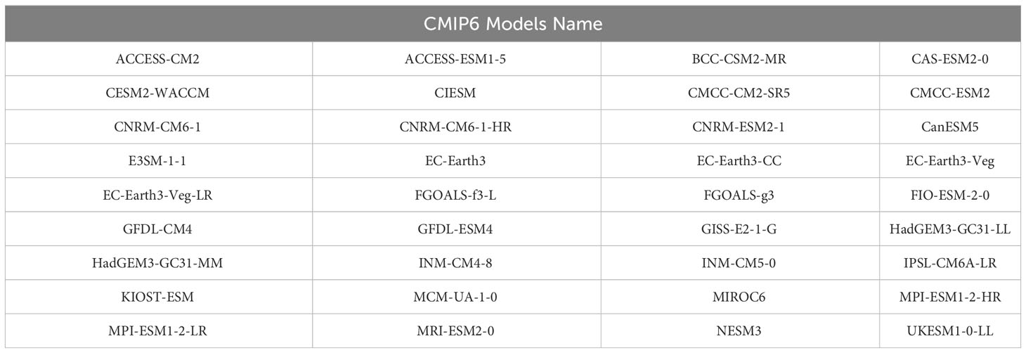
Table 1 The CMIP6 models.

3 The relationship between SST_H and ENSO in the simple model, observation, and CMIP6

3.1 The relationship in the recharge oscillator model

The role of tropical Pacific OHC in ENSO predictability is illustrated in Figure 2. According to the numerical solution of the simplest recharge oscillator model (Figure 2A; Burgers et al., 2005), OHC leads SST anomalies by about 6-9 months (Figure 2B), especially during the early calendar months of the year (Figure 2C), which is consistent with McPhaden (2003) using the observation data.

In recharge oscillator model, SST_H is in phase with H, as indicated by a correlation coefficient close to 1 (red line vs. blue line in Figure 2A). SST_H leads SST anomalies by about 6-9 months, which is also the same with H (Figure 2B). This suggests that SST_H can effectively represent H in this simple recharge oscillator model.

3.2 The relationship between observation and CMIP6 models

SST_H, WWV, and WWVw are predictors of SST anomalies. Firstly, WWV or WWVw leads SST anomalies by several months (blue or green line vs. black line in Figure 3A). For example, WWV or WWVw peaks before the SST anomalies reach their maximum in 1982. This point can be further found in Figure 3B. Consistent with Izumo et al. (2019), WWV leads SST by half a year, while WWVw has a longer lead time, especially for crossing the SPB (blue and green lines in Figure 3B). Meanwhile, the correlation coefficient between SST_H and WWV is 0.5 (significant at a 95% confidence level), which indicates that SST_H can also be a precursor for SST anomalies. The increase of SST_H in early spring suggests a recharge state in the tropical Pacific and the El Niño event may occur in the future (red and black lines in Figure 3A). SST_H always leads Niño3.4 SST by about 10 months (red line in Figure 3B). Among the 50 ENSO events from 1950 to 2022, 27 years were identified to be caused by SST_H signals. This finding is expected as SST_H is based on the subsurface temperature information. According to the recharge oscillator theory of ENSO, the time when OHC anomalies reach their maximum precedes the development of SST anomalies. For a longer lead time, the correlation between SST_H and the Niño3.4 index is higher than that of WWV. As shown in Figure 4, SST_H from January to March is a predictor for the following winter ENSO SST anomalies. Particularly, T = a_*SST_H+b, where T indicates winter SST anomalies and SST_H indicates the value of SST_H from January to March. Here, a=0.0402 and b=0.017 are trained by using observational data. The prediction skill of anomaly correlation coefficient (ACC) is 0.46, which is significant at a 99% confidence level. By using this index, the spring predictability barrier is weakened.

FIGURE 3

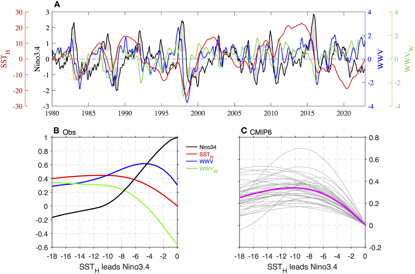
Figure 3 (A) Time series of SST_H (red line), WWV (blue line), WWVw (green line) and Niño3.4 index (black line) from 1980 to 2022. The gray shading means the Niño3.4 index exceeds ±0.5°C. (B) The autocorrelation of Niño3.4 SST anomalies and the cross-correlation between the Niño3.4 SST anomalies and WWV (blue line), WWVw (green line) and SST_H (red line) respectively for 1980–2017. (C) The cross correlation between the Niño3.4 SST anomalies and SST_H of 36 CMIP6 models (purple line and thin gray lines indicate the ensemble mean and each model results).

FIGURE 4

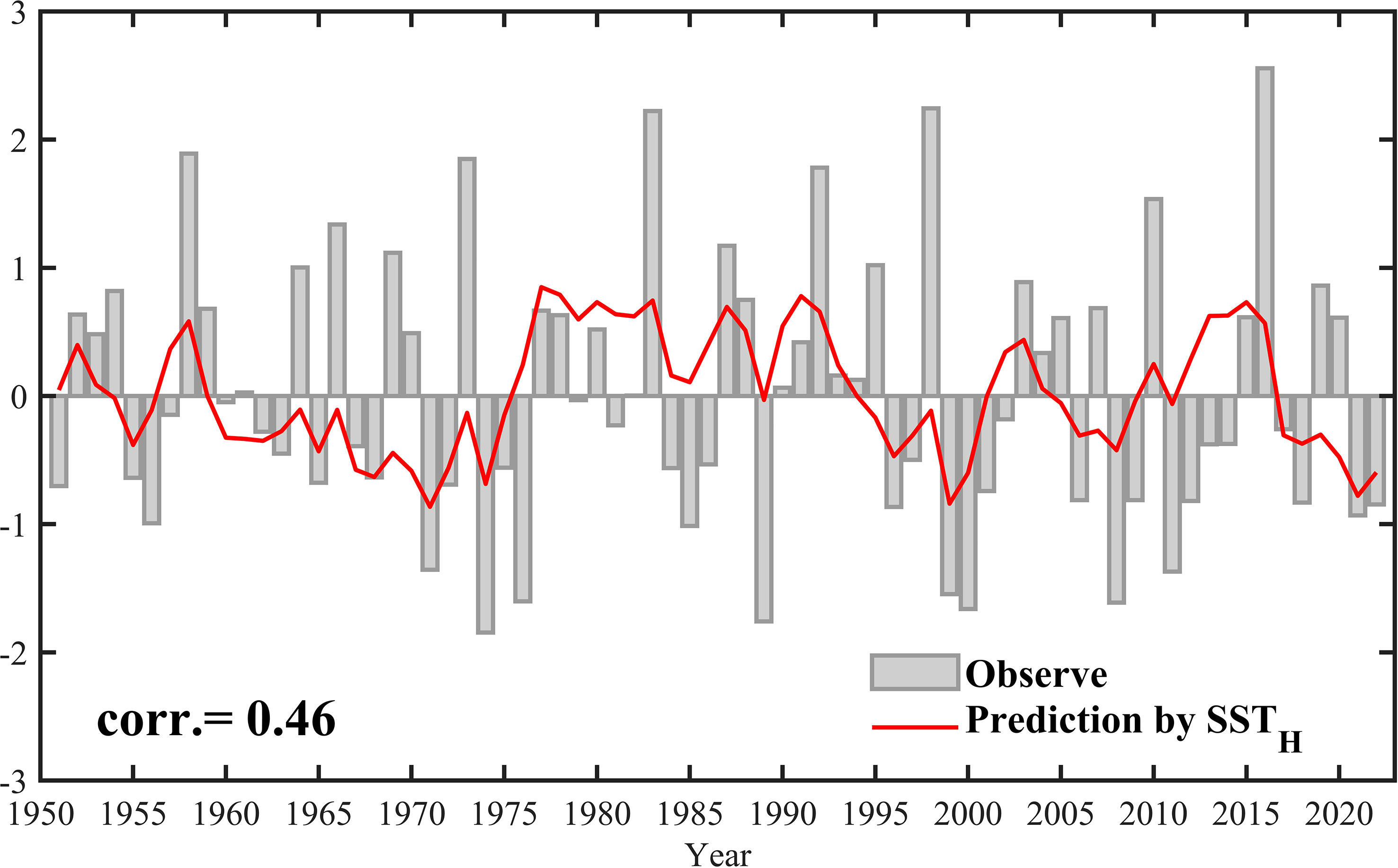
Figure 4 The observational averaged sea surface temperature anomalies in Niño3.4 area from December(0) to February(1) (gray bar), Predicted sea surface temperature anomalies by using SST_H from January(0) to March(0) (red Line).

The role of SST_H in ENSO prediction is also identified in the CMIP6 datasets. In 36 CMIP6 models, SST_H consistently leads Niño3.4 SST by about 6-16 months (gray lines in Figure 3C). The highest correlation is about 0.7. The multi-model ensemble (MME) mean of the 36 CMIP6 models shows that SST_H leads Niño3.4 SST by 10 months with the highest correlation (0.34; purple line in Figure 3C). This implies that SST_H can also act as a precursor for ENSO events in CMIP6 models, consistent with observation.

SST_H is effective in crossing ENSO SPB. The primary characteristic of the ENSO SPB is the occurrence of a band with the maximum decline of monthly autocorrelation in spring. This is evident from the monthly autocorrelation of SST anomaly variability and its lag gradient. It indicates that ENSO forecasting experiences the most rapid loss of predictability in spring (Figure 5A). Subsequently, persistent SST anomalies show higher skills for winter SST anomalies. However, SST_H still suggests a higher skill in the early spring (Figure 5B). When SST_H leads Niño3.4 SST anomaly about 10~16 months, their correlation is higher. Particularly, the cross-correlation between winter SST and 12 months earlier of SST_H is about 0.5, indicating that it is a superior predictor for crossing ENSO SPB compared to Niño 3.4 itself. Compared with SST_H, spring WWV exhibits a higher correlation with winter Niño3.4 (Figure 5C). This lead correlation coefficient is about 0.6, suggesting that WWV cannot be reflected entirely by SST_H. According to eq. (2.2), our index only reflects the low frequency of WWV. SST_H index is derived by eq. (2.2), which is the simplest relationship between T and WWV. Only by this simple relationship, we can use SST data to represent WWV. In fact, WWV is related to T and the damping of thermocline depth itself although the damping term is small (Burgers et al., 2005). As such, the WWV exhibits a higher correlation magnitude compared with SST_H. Note here although the WWV index is more effective in crossing ENSO SPB, our index can be utilized to identify the role of low frequency component of the subsurface in the tropical Pacific in ENSO prediction before 1980. Additionally, WWVw exhibits a longer lead time in ENSO prediction compared to WWV, which is consistent with Izumo et al. (2019) (Figure 5D).

FIGURE 5

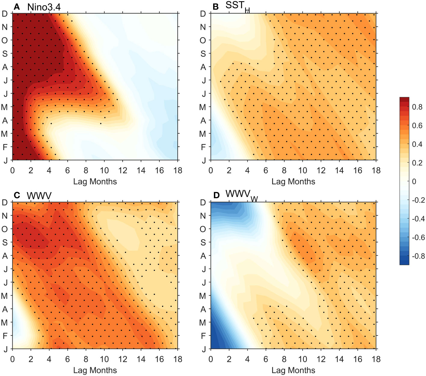
Figure 5 The autocorrelation map of (A) Niño3.4 index, the cross-correlation between the Niño3.4 index, and (B) SST_H, (C) WWV, (D) WWVw from 1980-2022. The vertical axis indicates the initial month. Dots indicate a significant correlation at a 90% confidence level.

4 The interdecadal modulation of the effectiveness of SST_H in ENSO prediction and possible mechanism

4.1 The interdecadal modulation of the effectiveness of in ENSO prediction

As mentioned in the previous sections, SST_H is a predictor for ENSO events, indicating the role of subsurface temperature in ENSO development and prediction. SST_H consistently leads SST anomalies by about 10 months, allowing it to cross ENSO SPB.

The effective role of the subsurface tropical Pacific, represented by SST_H, in ENSO development and prediction before 1980 is evident in Figure 6. SST_H has been a predictor since 1950 (red line in Figure 6A). For example, SST_H reached its maximum before an El Niño event occurred in 1958. This point can be further observed in Figure 6B. Since 1950, SST_H always leads SST anomalies by about 10 months (the correlation coefficient is about 0.4) so that can cross the SPB.

FIGURE 6

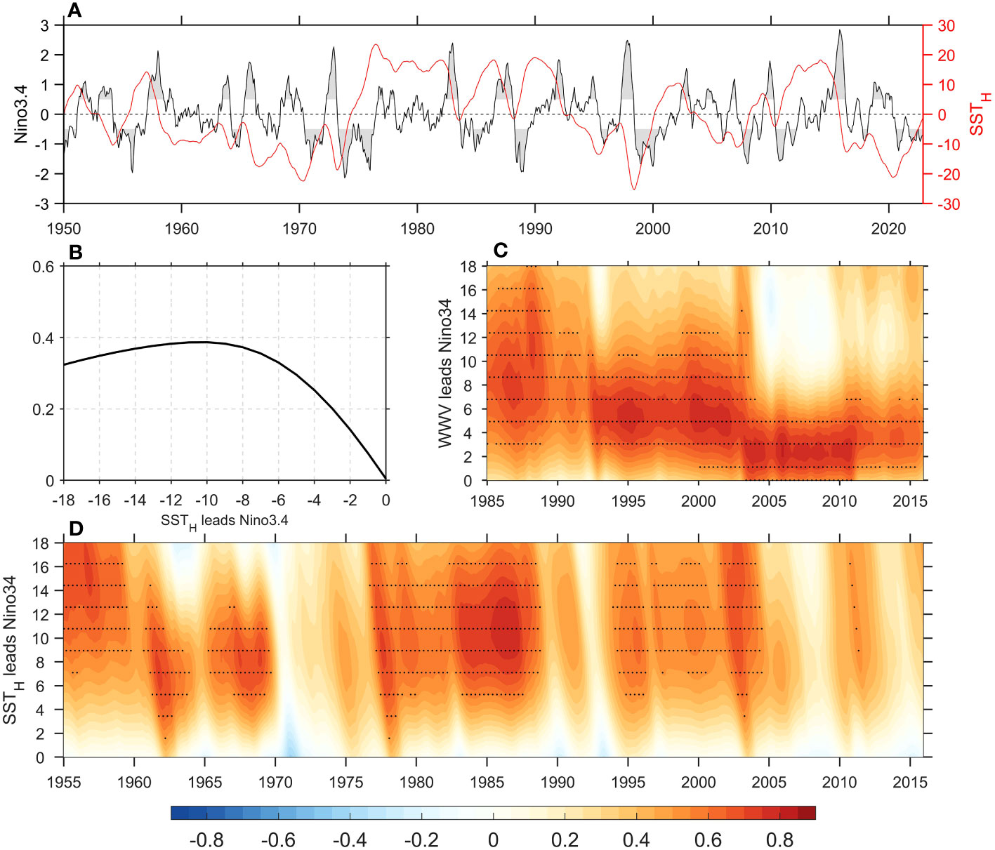
Figure 6 (A) Time series of SST_H (red line) and Niño3.4 index (black line) from 1950 to 2022. (B) The cross-correlation between SST_H and Niño3.4 SST anomalies (blue line) for 1950–2022. (C) Cross-correlation between the WWV and Niño3.4 indices as a function of WWV leads month (y-axis) and year (x-axis) within a 10‐year running window from 1985-2015. (D) Cross-correlation between the SST_H and Niño3.4 indices as a function of SST_H leads month (y-axis) and year (x-axis) within a 10‐year running window from 1955-2015. Dots represent a significant 10-year sliding correlation at a 90% confidence level.

The effectiveness of SST_H remains relatively stable on the interdecadal time scale. The correlation between the Niño3.4 index and SST_H, WWV exhibits an interdecadal change (Figures 6C, D). The correlation coefficient is higher when WWV leads Niño3.4 by about 4~8 months before 2000 (Figure 6C). However, the lead time of WWV in relation to Niño3.4 shortens to 0~4 months after 2000, indicating a weakened role of WWV in ENSO prediction, consistent with the previous study (McPhaden, 2012). For SST_H, the lead time roughly maintains at 10 months since 1985 (Figure 6D), suggesting that it is a relatively stable index for the lead time.

SST_H is more effective in predicting ENSO with a lead time of about 10 months compared with WWV and WWVw after the 21^st century (Figure 7). We divide the time period into two periods: 1980-1999 and 2000-2022. Before 2000, SST_H leads Niño3.4 SST anomalies by about 10 months (the correlation coefficient is about 0.6; N_e=28), while after 2000, the same lead time exhibits a lower correlation (the correlation coefficient is about 0.4; N_e=31). During the 1980-1999 period, WWV led Niño3.4 SST anomalies by about 6 months (the correlation coefficient is about 0.7; N_e=41). However, after 2000, this lead time is shortened to about 3 months, and the correlation decreases (lower than SST_H for lead time > 6 months; blue lines in Figure 7; N_e=63). Furthermore, the cross-correlation for WWVw decreases dramatically from 0.5 in 1980-1999 (N_e=41) to 0.15 in 2000-2022 (N_e=43), indicating reduced effectiveness of WWVw after 2000 (green lines in Figure 7). On the other hand, SST_H suggests a relatively smaller modulation compared to WWV and WWVw for crossing the SPB (red line in Figure 7).

FIGURE 7

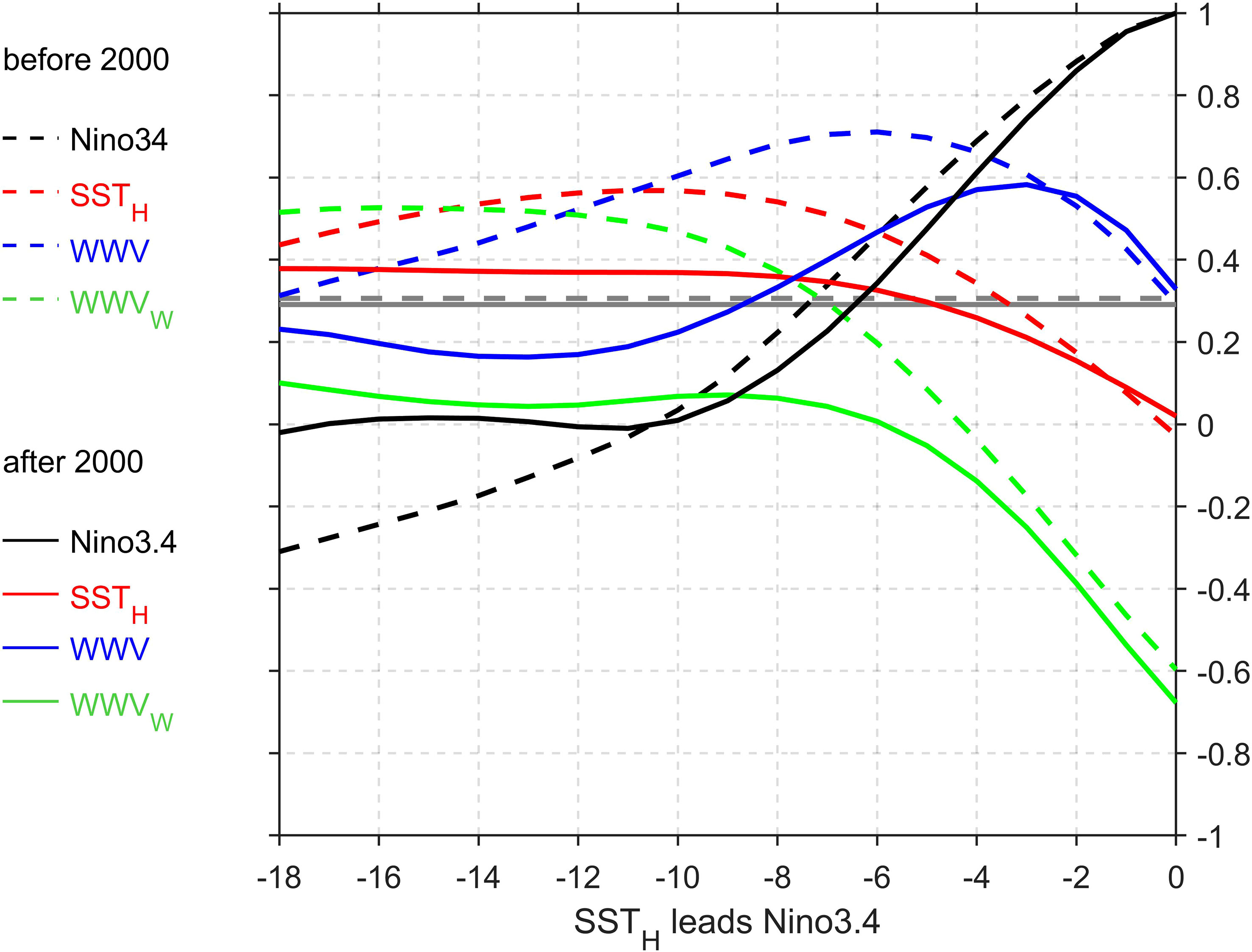
Figure 7 The autocorrelation of Niño3.4 SST anomalies (black lines) and the cross-correlation between the Niño3.4 SST anomalies and WWV (blue lines), WWVw (green lines), and SST_H (red lines) respectively for 1980-1999 and 2000-2022. Dark gray dashed and solid lines represent the critical correlations at 90% confidence levels respectively for 1980-1999 and 2000-2022.

SST_H is also more effective in crossing ENSO SPB after 2000. Before 2000, WWV was a predictor in the spring (Figure 8C). Although the in-phase relationship between WWV and SST is small (close to 0), spring WWV anomalies lead winter SST anomalies by 8-12 months (the correlation coefficient is about 0.7), indicating that it is a superior predictor for crossing ENSO SPB compared to Niño 3.4 itself (Figure 8A vs Figure 8C). Following spring, persistent SST anomalies exhibit higher skills in predicting winter SST anomalies (Figure 8A). Therefore, WWV is a constraint for forecasts starting early in the calendar year. Both SST_H and WWVw suggests a similar role in ENSO prediction, displaying higher skills for winter and following spring SST anomalies (Figures 8B, D). In the 21^st century, the SPB becomes more pronounced (Figure 8E). Spring WWV shows a smaller skill in predicting winter SST anomalies, and the lead time is notably shortened (Figure 8G), which is consistent with the findings of McPhaden (2012). WWVw also exhibits a dramatic drop in effectiveness (Figure 8H). While SST_H suggests a slightly lower skill in the early spring (Figure 8F), and the lead time remains consistent with that before 2000. The cross correlation between winter SST and 12 months earlier of SST_H is about 0.5, indicating that it is an effective predictor for crossing the SPB.

FIGURE 8

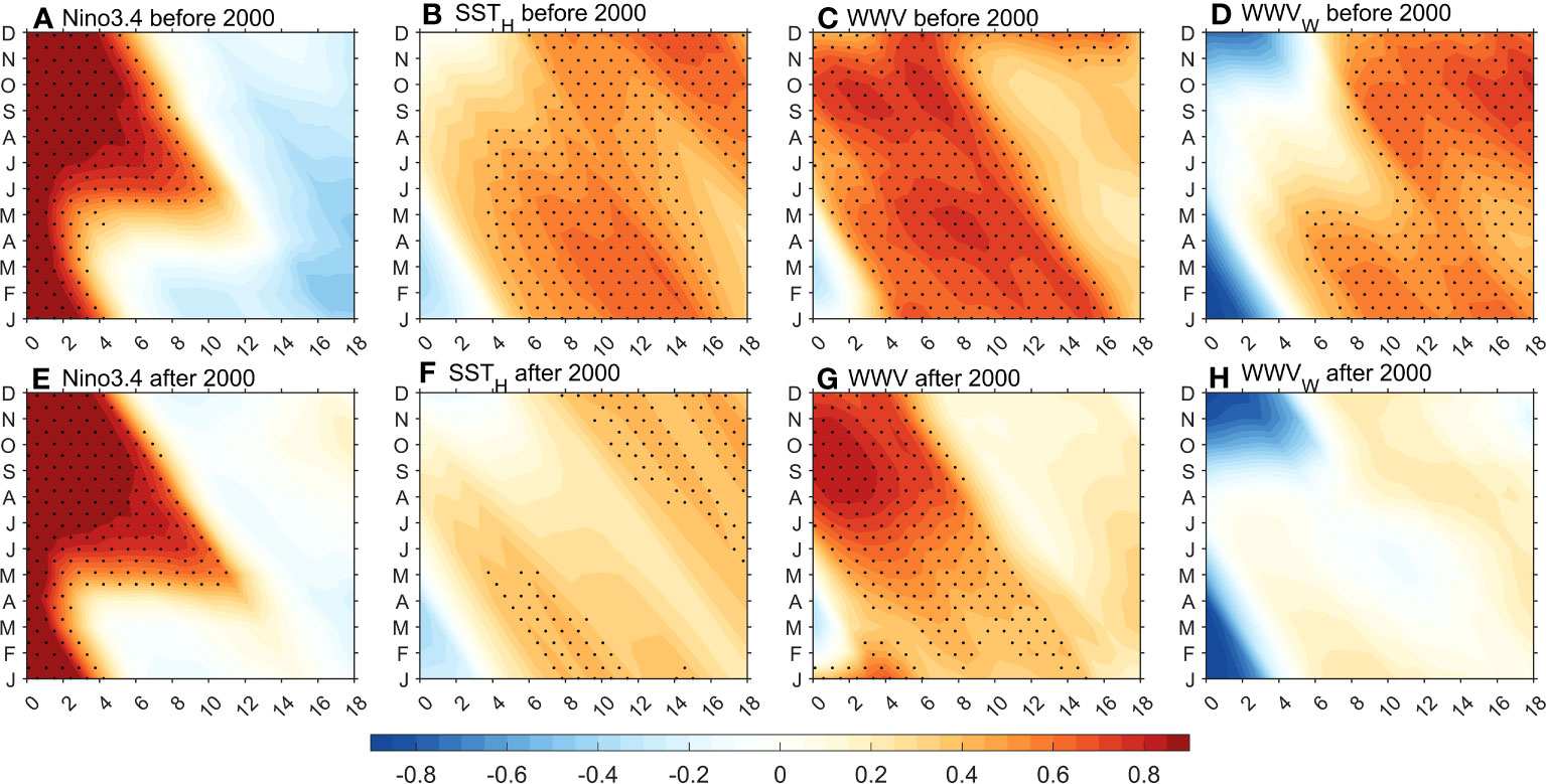
Figure 8 (A–D), (E–H) are the same as Figure 5, except for 1980-1999 and 2000-2022, respectively. Dots indicate a significant correlation at a 90% confidence level.

4.2 Possible mechanisms to explain the effectiveness of , WWV and WWVw after the 21st century

In this section, we will explain why SST_H becomes more effective after the 21^st century. Mathematically, if we assume the time series of T in the simplest case: T = sin(ω₀t) , according to eq. (2.2), the time series of H can be derived as H = cos(ω₀t). The lead-lag correlation (r_H,T(τ), τ>0 indicates H leads T for τ months) between H and T is:

$\begin{array}{ll}{r}_{H,T}(\tau )=\text{sin}({\omega }_0\text{τ})& \text{(4.1)}\end{array}$

According to eq. (4.1), the maximum cross-correlation occurs when τ equals 1/4 ENSO period (ENSO period is $\frac{2\pi }{{\omega }_0}$). When the ENSO period shortens, the lead time becomes smaller. The lead-lag cross-correlation relationship is controlled by the ENSO period (black lines in Figure 7), which can be theoretically derived from the recharge oscillator (Jin et al., 2021; their eq. (3.8)). A shortened ENSO period can lead to a decreased lead-lagged correlation. Note here other factors (e.g., the damping term of the WWV) can also lead to this lead-lag correlation as this theoretical solution is derived by the simplest recharge oscillator. Therefore, due to this model may be too simple, the relationship between lead-lag correlation and ENSO cycle is consistent with the observation before 2000 but not after 2000.

The shortened ENSO period after the 21^st century may contribute to the reduced effectiveness of WWV and WWVw. According to recharge oscillator theory, under the effect of westerly wind forcing, the accumulated warm water in the western Pacific flows eastward, finally affecting SST anomalies in the eastern Pacific (e.g., an El Niño event). At the same time, the zonally integrated Sverdrup transport, caused by wind stress, reduces the thermocline depth in the western Pacific (Wyrtki, 1985; Jin, 1997). During the period of 1980-1999, the positive correlation coefficient between thermocline depth and winter SST anomalies in the eastern Pacific can reach the west of 140°E with a lead time of 12 months (Figure 9A), indicating that the western Pacific is still “recharging” 12 months before an El Niño event happens. During this period, the region of OHC (e.g., WWV, 120°E~80°W) has a reasonable lead time of about 9 months since the major area of the Pacific exhibits positive correlation coefficients. However, the situation is different in the 21^st century. A negative correlation occurs in the western Pacific with a lead time of about 12 months (Figure 9B), indicating that the western Pacific is “discharging” at 12 months before an El Niño event occurs. This means that the OHC in the western Pacific is building up for a La Niña event at that lead time. It shows an accelerated recharge/discharge rate (a shortened ENSO period) after the 21^st century. The correlation coefficient of the west (east) of the dateline is negative (positive) at about 9 months lead, indicating that the area of WWV or WWVw is not appropriate. On the other hand, SST_H does not need to consider this situation as it is constructed using SST anomalies. The Niño3.4 area is able to represent the major feature of ENSO activity. This is why SST_H is more effective than WWV after the 21^st century.

FIGURE 9

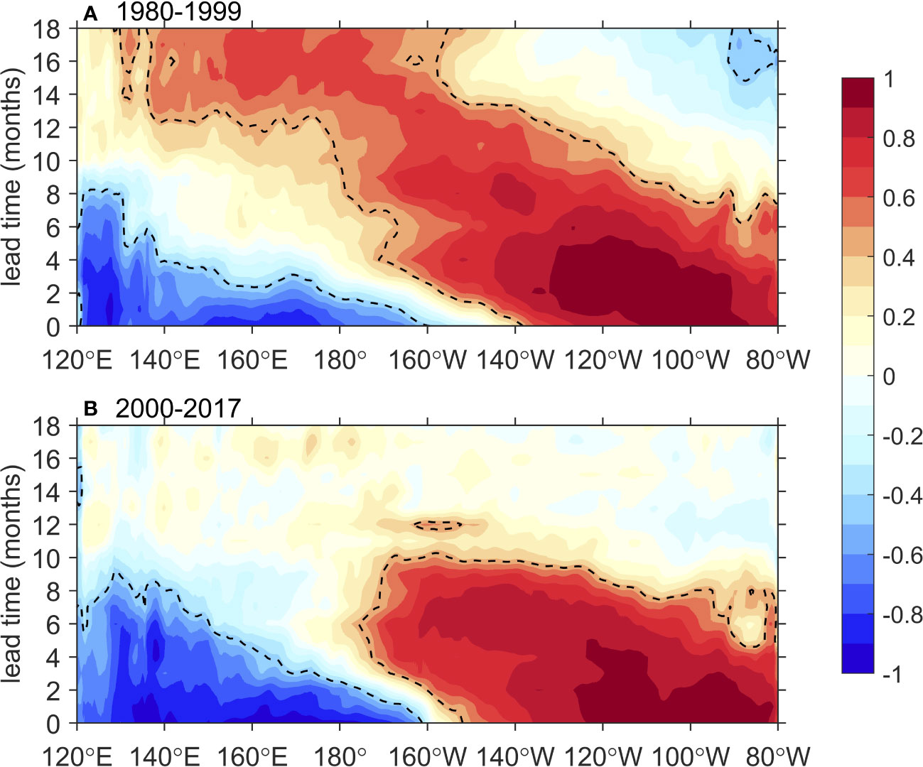
Figure 9 The lead-lag correlation between the Z₂₀ and winter (January) Niño3.4 index. Lead time > 0 indicates Z₂₀ leads winter Niño3.4 index from (A) 1980-1999 and (B) 2000-2017. The dashed line indicates the correlation coefficient between Z₂₀ and Niño3.4 index exceeding 95% confidence level.

It should be noted that SST_H, WWV and WWVw are all less effective after the 21^st century (dashed vs. solid lines in Figure 7). According to eq. (4.1), the lead time is directly related to the ENSO period. As the ENSO period is longer during 1980-1999 (McPhaden, 2012), the OHC-based indexes are more effective, meaning that ENSO predictability is higher. In this section, we have shown that due to the accelerated recharge/discharge after the 21^st century, WWV and WWVw have become less effective. However, as SST_H is constructed by SST anomalies, it remains relatively effective compared to WWV and WWVw after the 21^st century.

5 Summary and discussion

This paper aims to investigate an SST-constructed index that utilizes SST data to represent subsurface OHC in the tropical Pacific for crossing ENSO SPB. According to the relationship between tropical Pacific OHC and eastern SST anomalies (eq. (2.2)), subsurface OHC can be represented by Niño3.4 SST anomalies. This index leads winter SST anomalies by about 10 months, indicating that it is a constraint in crossing ENSO SPB. Compared to WWV or WWVw, this index remains stable and more effective after the 21^st century. Due to the accelerated recharge/discharge rate (ENSO period is shortened) after the 2000s, the effectiveness of the OHC region of OHC (WWV or WWVw) for winter SST anomalies at large lead times is diminished. On the other hand, since SST_H is constructed only by SST anomalies and the Niño3.4 region can represent the major features of ENSO activities, SST_H still leads winter SST anomalies by 10 months. Additionally, even though ocean subsurface data (e.g., WWV) is not reliable before 1980, SST_H can be employed to explore the interdecadal modulation of the relationship between subsurface and SST anomalies.

The SST_H is able to identify the effectiveness of the subsurface information in the tropical Pacific in crossing ENSO SPB. Reliable subsurface information is not available before 1980, and some climate models (e.g., CMIP6) lack output data for the ocean subsurface. Therefore, we can use this index to explore the lead-lag relationship between ocean subsurface information and ENSO SST anomalies. Moreover, SST_H may also play a role in the ENSO forecast after the 21^st century. The lead correlation between SST_H and the Niño3.4 index is higher than that between WWV and the Niño3.4 index for longer lead times (> 10 months). In summary, SST_H can be used to estimate the oceanic subsurface temperature to predict ENSO. Moreover, we find this index is more stable in predicting ENSO events.

This study provides an explanation as to why using SST data alone can lead to success in understanding ENSO and its predictability. We suggest that SST data contains information about the subsurface in the tropical Pacific. For example, a linear inverse model (LIM) using tropical SSTs can investigate many features of observed seasonal tropical SST variability and predictability (Penland and Sardeshmukh, 1995). It should be noted here that the relationship between OHC and SST indicated by eq. (2.2) is not so realistic. Eq. (2.2) suggests that the vertically averaged heat transport into and out of the equatorial region is accomplished via Sverdrup transport. It assumes that the anomalous off-equatorial wind stress curl responsible for the Sverdrup transport is proportional to the zonal equatorial wind stress anomaly (Stein et al., 2010). Here, we neglect the damping term of OHC itself, which is a relatively small term according to Burgers et al. (2005). In addition, because SST_H is not very sensitive to the ENSO period, its correlation with ENSO has better stability, which is an advantage of SST_H. However, it also makes SST_H less suitable for predicting every ENSO event.

Data availability statement

The original contributions presented in the study are included in the article/supplementary material. Further inquiries can be directed to the corresponding author.

Author contributions

All authors contributed to the study conception and design. LZ, YJ and LW contributed to the study’s conception and design. Material preparation, data collection and analysis were performed by XM, HC and LZ. The first draft of the manuscript was written by XM and HC and all authors commented on previous versions of the manuscript. All authors read and approved the final manuscript.

Funding

This work is supported by the National Natural Science Foundation of China (42206013) and the Strategic Priority Research Program of the Chinese Academy of Sciences (XDB40000000).

Conflict of interest

The authors declare that the research was conducted in the absence of any commercial or financial relationships that could be construed as a potential conflict of interest.

Publisher’s note

All claims expressed in this article are solely those of the authors and do not necessarily represent those of their affiliated organizations, or those of the publisher, the editors and the reviewers. Any product that may be evaluated in this article, or claim that may be made by its manufacturer, is not guaranteed or endorsed by the publisher.

References

Anderson B. T. (2007). On the joint role of subtropical atmospheric variability and equatorial subsurface heat content anomalies in initiating the onset of ENSO events. J. Climate 20 (8), 1593–1599. doi: 10.1175/JCLI4075.1

CrossRef Full Text | Google Scholar

Balmaseda M. A., Davey M. K., Anderson D. L. (1995). Decadal and seasonal dependence of ENSO prediction skill. J. Climate 8 (11), 2705–2715. doi: 10.1175/1520-0442(1995)008<2705:DASDOE>2.0.CO;2

CrossRef Full Text | Google Scholar

Barnston A. G., Tippett M. K., L'Heureux M. L., Li S., DeWitt D. G. (2012). Skill of real-time seasonal ENSO model predictions during 2002–11: Is our capability increasing? Bull. Am. Meteorol. Soc. 93 (5), 631–651. doi: 10.1175/BAMS-D-11-00111.1

CrossRef Full Text | Google Scholar

Bretherton C. S., Widmann M., Dymnikov V. P., Wallace J. M., Bladé I. (1999). The effective number of spatial degrees of freedom of a time-varying field. J. Climate 12, 1990–2009. doi: 10.1175/1520-0442(1999)012<1990:TENOSD>2.0.CO;2

CrossRef Full Text | Google Scholar

Bunge L., Clarke A. J. (2014). On the warm water volume and its changing relationship with ENSO. J. Phys. Oceanogr. 44 (5), 1372–1385. doi: 10.1175/JPO-D-13-062.1

CrossRef Full Text | Google Scholar

Burgers G., Jin F. F., Van Oldenborgh G. J. (2005). The simplest ENSO recharge oscillator. Geophys. Res. Lett. 32 (13), L13706. doi: 10.1029/2005GL022951

CrossRef Full Text | Google Scholar

Carton J. A., Giese B. S. (2008). A reanalysis of ocean climate using Simple Ocean Data Assimilation (SODA). Monthly Weather Rev. 136 (8), 2999–3017. doi: 10.1175/2007MWR1978.1

CrossRef Full Text | Google Scholar

Chen W., Lu R., Ding H. (2022). A decadal intensification in the modulation of spring western tropical Atlantic sea surface temperature to the following winter ENSO after the mid-1980s. Clim. Dyn. 59 (11-12), 3643–3655. doi: 10.1007/s00382-022-06288-z

CrossRef Full Text | Google Scholar

Chen H. C., Tseng Y. H., Hu Z. Z., Ding R. (2020). Enhancing the ENSO predictability beyond the spring barrier. Sci. Rep. 10 (1), 984. doi: 10.1038/s41598-020-57853-7

PubMed Abstract | CrossRef Full Text | Google Scholar

Ding R., Li J., Tseng Y. H., Sun C., Guo Y. (2015). The Victoria mode in the North Pacific linking extratropical sea level pressure variations to ENSO. J. Geophys. Res.: Atmos. 120 (1), 27–45. doi: 10.1002/2014JD022221

CrossRef Full Text | Google Scholar

Eyring V., Bony S., Meehl G. A., Senior C. A., Stevens B., Stouffer R. J., et al. (2016). Overview of the Coupled Model Intercomparison Project Phase 6 (CMIP6) experimental design and organization. Geosci. Model. Dev. 9, 1937–1958. doi: 10.5194/gmd-9-1937-2016

CrossRef Full Text | Google Scholar

Ham Y. G., Kug J. S., Park J. Y. (2013). Two distinct roles of Atlantic SSTs in ENSO variability: North tropical Atlantic SST and Atlantic Niño. Geophys. Res. Lett. 40 (15), 4012–4017. doi: 10.1002/grl.50729

CrossRef Full Text | Google Scholar

Huang B., Thorne P. W., Banzon V. F., Boyer T., Zhang H. M., Lawrimore J. H., et al. (2017). Extended Reconstructed Sea Surface Temperature, version 5 (ERSSTv5): Upgrades, validations, and intercomparisons. J. Climate 30 (20), 8179–8205. doi: 10.1175/JCLI-D-16-0836.1

CrossRef Full Text | Google Scholar

Izumo T., Lengaigne M., Vialard J., Suresh I., Planton Y. (2019). On the physical interpretation of the lead relation between Warm Water Volume and the El Niño Southern Oscillation. Clim. Dyn. 52 (5), 2923–2942. doi: 10.1007/s00382-018-4313-1

CrossRef Full Text | Google Scholar

Jin F.-F. (1997). An equatorial ocean recharge paradigm for ENSO. Part I: Conceptual model. J. Atmos. Sci. 54 (7), 811–829. doi: 10.1175/1520-0469(1997)054<0811:AEORPF>2.0.CO;2

CrossRef Full Text | Google Scholar

Jin Y., Liu Z., McPhaden M. J. (2021). A theory of the spring persistence barrier on ENSO. Part III: The role of tropical Pacific Ocean heat content. J. Climate 34 (21), 8567–8577. doi: 10.1175/JCLI-D-21-0070.1

CrossRef Full Text | Google Scholar

Jin Y., Lu Z., Liu Z. (2020). Controls of spring persistence barrier strength in different ENSO regimes and implications for 21st century changes. Geophys. Res. Lett. 47 (11), e2020GL088010. doi: 10.1029/2020GL088010

CrossRef Full Text | Google Scholar

Levine A. F., McPhaden M. J. (2015). The annual cycle in ENSO growth rate as a cause of the spring predictability barrier. Geophys. Res. Lett. 42 (12), 5034–5041. doi: 10.1002/2015GL064309

CrossRef Full Text | Google Scholar

Liu Z., Jin Y., Rong X. (2019). A theory for the seasonal predictability barrier: threshold, timing, and intensity. J. Climate 32 (2), 423–443. doi: 10.1175/JCLI-D-18-0383.1

CrossRef Full Text | Google Scholar

McPhaden M. J. (2003). Tropical Pacific Ocean heat content variations and ENSO persistence barriers. Geophys. Res. Lett. 30 (9), 1480. doi: 10.1029/2003GL016872

CrossRef Full Text | Google Scholar

McPhaden M. J. (2012). A 21st century shift in the relationship between ENSO SST and warm water volume anomalies. Geophys. Res. Lett. 39 (9), 3439. doi: 10.1029/2012GL051826

CrossRef Full Text | Google Scholar

McPhaden M. J., Zebiak S. E., Glantz M. H. (2006). ENSO as an integrating concept in earth science. Science 314 (5806), 1740–1745. doi: 10.1126/science.1132588

PubMed Abstract | CrossRef Full Text | Google Scholar

Meinen C. S., McPhaden M. J. (2000). Observations of warm water volume changes in the equatorial Pacific and their relationship to El Niño and La Niña. J. Climate 13 (20), 3551–3559. doi: 10.1175/1520-0442(2000)013<3551:OOWWVC>2.0.CO;2

CrossRef Full Text | Google Scholar

Nigam S., Sengupta A. (2021). The full extent of El Niño's precipitation influence on the United States and the Americas: The suboptimality of the Niño 3.4 SST index. Geophys. Res. Lett. 48 (3), e2020GL091447. doi: 10.1029/2020GL091447

CrossRef Full Text | Google Scholar

Penland C., Sardeshmukh P. D. (1995). The optimal growth of tropical sea surface temperature anomalies. J. Climate 8 (8), 1999–2024. doi: 10.1175/1520-0442(1995)008<1999:TOGOTS>2.0.CO;2

CrossRef Full Text | Google Scholar

Planton Y., Vialard J., Guilyardi E., Lengaigne M., Izumo T. (2018). Western Pacific Oceanic heat content: A better predictor of la niña than of el niño. Geophys. Res. Lett. 45 (18), 9824–9833. doi: 10.1029/2018GL079341

CrossRef Full Text | Google Scholar

Ren H. L., Jin F. F., Tian B., Scaife A. A. (2016). Distinct persistence barriers in two types of ENSO. Geophys. Res. Lett. 43 (20), 10973–10979. doi: 10.1002/2016GL071015

CrossRef Full Text | Google Scholar

Seleznev A., Mukhin D. (2023). Improving statistical prediction and revealing nonlinearity of ENSO using observations of ocean heat content in the tropical Pacific. Clim. Dyn. 60 (1-2), 1–15. doi: 10.1007/s00382-022-06298-x

CrossRef Full Text | Google Scholar

Shi L., Ding R., Hu S., Li J., Tseng Y., Li X. (2022). Influence of the North Pacific Victoria mode on the spring persistence barrier of ENSO. J. Geophys. Res.: Atmos. 127 (9), e2021JD036206. doi: 10.1029/2021JD036206

CrossRef Full Text | Google Scholar

Stein K., Schneider N., Timmermann A., Jin F.-F. (2010). Seasonal Synchronization of ENSO Events in a Linear Stochastic Model. J. Climate. 23 (21), 5629–5643. doi: 10.1175/2010JCLI3292.1

CrossRef Full Text | Google Scholar

Torrence C., Webster P. J. (1998). The annual cycle of persistence in the El Nño/Southern Oscillation. Q. J. R. Meteorol. Soc. 124 (550), 1985–2004. doi: 10.1002/qj.49712455010

CrossRef Full Text | Google Scholar

Wyrtki K. (1985). Water displacements in the Pacific and the genesis of El Niño cycles. J. Geophys. Res.: Oceans 90 (C4), 7129–7132. doi: 10.1029/JC090iC04p07129

CrossRef Full Text | Google Scholar

Yu J. Y., Kao H. Y. (2007). Decadal changes of ENSO persistence barrier in SST and ocean heat content indices: 1958–2001. J. Geophys. Res.: Atmos. 112 (D13), D13106. doi: 10.1029/2006jd007654

CrossRef Full Text | Google Scholar

Zhu J., Huang B., Zhang R. H., Hu Z. Z., Kumar A., Balmaseda M. A., et al. (2014). Salinity anomaly as a trigger for ENSO events. Sci. Rep. 4 (1), 6821. doi: 10.1038/srep06821

PubMed Abstract | CrossRef Full Text | Google Scholar