 Michelle Linklater
 Bradley D. Morris
 David J. Hanslow
- Water, Wetlands and Coastal Science, Department of Planning and Environment, Sydney, NSW, Australia
The increasing availability and quality of high-resolution bathymetry data has led to a growing need for automated classification approaches to extract seabed features and better understand our ever-changing and complex seascapes. Here we present a new set of GIS tools designed to classify seabed landforms on continental and island shelf settings. The classification approach utilises bathymetry data and its derivatives of slope, ruggedness and bathymetric position index to delineate key components of the seabed surface. The user is guided through a series of steps to break down the seabed surface into components termed ‘surface elements’ (e.g. smooth, rugose, slope areas), which are subsequently grouped into prominent seabed features termed ‘seabed landforms’ (e.g. reefs, channels, scarps). Manual review and editing are incorporated into the workflow, striking a balance between automation and expert manual interpretation. We present the toolset using examples from the statewide marine lidar dataset from New South Wales, Australia, and explore tool settings using bathymetric data representing different data sources (multibeam and marine lidar), environmental seascapes, data resolutions (2, 5, 10 and 20 m cell size) and data preparation treatments (with and without data smoothing). The GIS toolset presented offers an effective and flexible method to extract key features from high-resolution shelf bathymetry data. Such mapping provides fundamental baseline data for vast applications within marine planning, research and management.
1 Introduction
An understanding of the presence, extent and configuration of features submerged within a seascape is critical to effectively managing the marine environment. Knowledge of prominent features such as reef outcrops or sediment plains is crucial information for coastal hazard management, marine spatial planning, fisheries management and benthic habitat mapping among a vast range of cross-disciplinary applications (Brown et al., 2012; Hanslow et al., 2016; Porskamp et al., 2018; Kinsela et al., 2022). As sea-level rise accelerates and storm impacts increase with climate change, there is an urgent need for detailed seabed data to help understand and manage coastal hazards which are projected to increase dramatically over future decades (Oppenheimer et al., 2019). With growing anthropogenic pressures on the marine environment, a baseline understanding of the features occurring within a region is crucial for marine estate management in the present-day as well as managing for change over time (Brown et al., 2012).
Seabed bathymetry data forms a foundational product from which the structure of the seafloor can be “seen”, and it is collected in increasing detail as technology improves over time. The growing acquisition of bathymetry data has in turn prompted a growing field of marine geomorphometry – which focuses on the quantitative analysis of digital elevation models (DEMs), including the extraction of terrain variables and discrete features from the seabed surface (Pike, 2000; Lecours et al., 2016). The delineation of seabed features can be connected, with ground-truthing data (e.g. underwater video, sediment samples), to seafloor composition to generate benthic habitat maps and geomorphology interpretations which inform marine planning, management, and research (Brown et al., 2012; Harris and Baker, 2020).
The availability of bathymetric data is ever-increasing due to concerted efforts to increase mapping coverage on regional (e.g. Australian HydroScheme Industry Partnership Program, Houston, 2020) and global scales (e.g. Nippon Foundation-GEBCO Seabed 2030, Mayer et al., 2018; Wölfl et al., 2019) and to generate wide-scale, integrated seabed classifications (Harris et al., 2014; Thorsnes et al., 2018; Lucieer et al., 2019; Sowers et al., 2020). With greater volumes of data capture, there is a rapidly growing need for efficient and effective methods of interpreting and classifying seabed features. Methods of manual digitisation of features are increasingly impractical as the scale and frequency of data collection exceeds the time required to manually interpret and classify, and users instead look to semi-automated approaches. While many tools and approaches are available to perform semi-automated classification procedures, the diversity of seabed features and varied program objectives globally mean that it’s challenging to find a one-size-fits-all approach.
There is evolving discussion around the development and application of standardised classification approaches to enable comparisons and integration of disparate datasets (Lecours et al., 2016; Dove et al., 2019). A number of widely used classification schemes have been developed (Greene et al., 1999; Federal Geographic Data Committee, 2012; Galparsoro et al., 2012; IHO, 2019) although many studies still customise classification schemes for features and habitats for their specific survey area and project focus (Harris and Baker, 2020). Progress on unifying feature terms is continuing to occur with the compilation of standardised terminologies for seabed features (e.g. Dove et al., 2020; Harris and Baker, 2020; Nanson et al., 2023). As these nomenclatures are increasingly adopted, users will in turn require standardised methodologies to define features consistently across studies. To enable users to readily explore marine geomorphometry and generate maps representing prominent seabed features, there is a pressing need for tools which allow users to implement semi-automated methods to define seabed features (Lecours et al., 2016; Dove et al., 2019). Importantly, these tools should be accessible to a range of users of varied backgrounds and GIS expertise (Lecours et al., 2016).
To effectively map seabed features within a seascape, a wide range of derivatives of bathymetry data, as well as varied spatial scales of analysis, have been explored (Diesing et al., 2016; Lecours et al., 2017; Misiuk et al., 2021). A broad range of techniques can be applied, as reviewed by (Lecours et al., 2016), including geostatistical and machine learning approaches, with object-based image analysis (OBIA) methods increasingly being adopted (Diesing et al., 2014; Lecours et al., 2016; Dekavalla and Argialas, 2017; Lecours et al., 2018; Janowski et al., 2022). Such approaches can incorporate other input datasets such as backscatter data or ground-truthing samples. This can present challenges as this data may not be available or consistently collected across the survey area (Lamarche and Lurton, 2017). Unlike bathymetry data, which can be standardised to international hydrographic guidelines (IHO, 2022), backscatter data currently lacks standardisation procedures to enable different surveys to be objectively compared (Lamarche and Lurton, 2017). Ground-truthing samples, such as sediment grabs or underwater video, are important for the validation of interpreted features, however they can be logistically difficult to collect over expansive areas. The scale of ground-truthing samples may also not appropriately match the scale of bathymetry data to enable extrapolation across broad spatial areas (Post, 2008).
Characterising the seabed using only the bathymetry is an appealing first product of seabed interpretation as this is the foundational dataset which most users will have acquired and it is able to be standardised. Bathymetry data enables a morphology-level classification, defining features based on surface shape (e.g. Dove et al., 2020). Such features have been termed ‘geoforms’, ‘bathymorphons’, ‘geomorphons’, ‘morphometric objects’ and ‘landforms’ across other studies (Federal Geographic Data Committee, 2012; Jasiewicz and Stepinski, 2013; Dekavalla and Argialas, 2017; Di Stefano and Mayer, 2018; Masetti et al., 2018; Linklater et al., 2019; Sowers et al., 2020). This classification of seabed morphologies may be undertaken as a non-overlapping, whole-seascape classification approach using specific tools, such as the classification dictionary in Benthic Terrain Modeler (Walbridge et al., 2018) or BRESS landform classifier (Masetti et al., 2018). Alternatively, a selection of different methods may be employed to capture individual features, which are then combined to build a complete classification of the seabed (e.g. Harris et al., 2014; Johnson et al., 2017).
Many classification approaches utilise the bathymetric position index (BPI), or similar measures, which calculate the relative height of features within a seascape, as a key metric to extract landform elements (Lundblad et al., 2006; Elvenes et al., 2014; Harris et al., 2014; Walbridge et al., 2018; Huang et al., 2022; Nanson et al., 2022). BPI has been incorporated into popular tools such as Benthic Terrain Modeler (Walbridge et al., 2018) which has been used to capture seabed features across a range of environments (e.g. Subarno et al., 2016; Goes et al., 2019; Lavagnino et al., 2020; Menandro et al., 2020). Rugosity and other variables of surface complexity (e.g. ‘terrain ruggedness’, Walbridge et al., 2018) have been recognised as effective at capturing shelf outcrops, and have been incorporated as an independently calculated measure overlain onto a Benthic Terrain Modeler classification (e.g. Lundblad et al., 2006; Linklater et al., 2019; De Oliveira et al., 2020).
In the New South Wales (NSW) context, on the southeast Australian continental shelf, a landmark statewide marine lidar dataset was collected in 2018, covering 4,000 km2 of seabed along a 2,000 km coastline (New South Wales Department of Planning and Environment, 2019). This data was acquired under the NSW Department of Planning and Environment statewide mapping program SeaBed NSW, which collects high-resolution bathymetric data to provide foundational data to improve modelling of coastal processes and hazards and inform assessments of coastal risk (Hanslow et al., 2016; Kinsela et al., 2017). The program includes acquisition of multibeam echosounder data, which builds upon an extensive catalogue of multibeam surveys since 2005 (Jordan et al., 2010). Previous methods to classify seabed features within these datasets were primarily manually digitised (Jordan et al., 2010), however with the high volumes of bathymetric data this is untenable, and there was clear need for greater automation.
The extraction of shelf reef features is a priority objective of the SeaBed NSW program to inform coastal hazard assessments and refine modelling of shoreline change based on an improved understanding of seafloor geomorphology and connectivity with sediment compartments (Hanslow et al., 2016; Kinsela et al., 2017; Kinsela et al., 2022). To conduct systematic mapping of features, particularly rocky reefs, at a statewide scale, a number of criteria needed to be met. The methodology must: incorporate semi-automated procedures; be applicable at a statewide scale; use accepted approaches within the seabed mapping community; use accessible software to enable ongoing use of the procedure over time; and provide a consistent approach to enable statistical comparisons along the NSW coast.
Linklater et al. (2019) conducted a pilot study of classification methods for the SeaBed NSW program, including a classification of seabed ‘landforms’ which define the key morphological features of the seascape. Ruggedness was shown to be a key measure in capturing shelf reefs within this southeast Australian shelf setting, out-performing other comparable measures for reef definition, standard deviation and range, which were shown to over-estimate reef extent. Linklater et al. (2019) adapted the Benthic Terrain Modeler (BTM) framework (Walbridge et al., 2018) to substitute ruggedness for depth, in order to capture rocky reefs. Despite the effectiveness of ruggedness in capturing reefs in this shelf setting, the ruggedness variable can present challenges when used to classify remotely sensed datasets as noise and motion artefacts may erroneously be classified as reef outcrops. This can be time consuming to manually correct, particularly when applied across wide-scale datasets. While the selected variables were effective, the framework presented by Linklater et al. (2019) to classify seabed landforms remained too manual to apply at broader scales, such as the NSW statewide marine lidar dataset.
To overcome these challenges and build in greater automation, we have adapted the framework presented in Linklater et al. (2019) into a semi-automated classification toolbox, the ‘Seabed Landforms Classification Toolset’, which focuses on defining seabed landforms within continental and island shelf settings. It translates the methodological approach outlined in Linklater et al. (2019) into sequential classification tools developed within an ArcGIS environment, which guides the user through the classification. Commonly used variables including slope, bathymetric position index (BPI) and ruggedness are utilised to characterise the seabed. The incorporation of ruggedness creates a targeted application for shelf environments where reef outcrops may be the prominent features observed. Procedures are implemented to address inherent noise artefacts and identify the full extent of reef outcrops. Nomenclature is introduced to characterise the seabed features using a suite of terms including reefs/banks, scarps, peaks, plains, depressions and channels. These terms capture the key components of the seascape, providing detail on the structure and expression of features while also balancing a more limited set of terms which group features with similar morphologies.
This study aims to: 1) describe the tools and procedures of the Seabed Landforms Classification Toolset; and 2) demonstrate the application of the toolset to varied scenarios of data types and environments. These tools can be utilised by the seabed mapping community to generate semi-automated classifications of shelf environments and apply a more detailed suite of terms to describe shelf features, with a particular focus on shelf and nearshore reefs. With an ever-expanding global repository of bathymetric data, together with an increased interest from the seabed mapping community to apply semi-automated procedures for seabed classification, this toolset aims to address the growing need for user-friendly approaches to readily classify seabed features. It provides a classification approach that is versatile to the needs of individual survey or program requirements, balancing automation and expert interpretation. The resulting whole-landscape classification product allows users to better understand our complex marine environments and provides detailed information to improve predictions of potential climate change impacts now and into the future.
2 Materials and methods
The Seabed Landforms Classification Toolset presented here was developed for SeaBed NSW, a statewide seabed mapping program conducted by the New South Wales (NSW) Department of Planning and Environment (formerly Office of Environment and Heritage). This program, initiated in 2017, aims to collect and analyse marine lidar and multibeam echosounder data along the NSW coast to characterise seabed composition for coastal hazard management and marine estate planning (Hanslow et al., 2016; Kinsela et al., 2022). Under this program, marine lidar data was acquired in 2018 along the ~2,000 km NSW coastline, in conjunction with ongoing multibeam echosounder mapping of selected regions. The mapping program focuses on the nearshore and inner continental shelf seabed, targeting water depths down to 60 m generally and extending deeper down to 100 m depending on survey requirements.
Prominent features of the NSW continental shelf seabed include temperate rocky reef outcrops (Jordan et al., 2010), and therefore the classification approach adopted needed to adequately capture outcropping reef features. Understanding the occurrence and extent of outcropping reef features is critical to understanding coastal processes and hazards at local and regional scales (see e.g. Kinsela et al., 2017; Kinsela et al., 2022), as well as informing marine planning and management.
2.1 Bathymetry data
High resolution (5 m cell size) statewide marine lidar data was collected along the entire NSW coastline by Fugro in 2018, commissioned by DPE (Table 1). Topographic and bathymetric lidar surveys resulted in 6,900 km2 of data of coastal land (at least 200 m inland of the shoreline) and nearshore waters. For this study, only bathymetry data was utilised and therefore the lidar dataset was clipped to 0 m elevation (Australian Height Datum). The lidar bathymetry covers 4,000 km2 and extends offshore to an average of 35 m depth (maximum 50 m depth) and an average distance of 3 km offshore (maximum 9 km). This data (and associated metadata) can be viewed on SEED NSW environmental data portal (New South Wales Department of Planning and Environment, 2019) or downloaded from the ELVIS Elevation and Depth Spatial Data Portal.
The NSW marine lidar dataset was used in this study to expand upon seabed classification methods piloted by Linklater et al. (2019) and translate the framework into a functional and versatile set of classification tools. The NSW marine lidar dataset was used to explore appropriate settings for the seabed classification toolset as the statewide dataset covers a variety of nearshore and shelf seabed environments. Selected areas within the marine lidar dataset were utilised in this study to demonstrate the classification toolset, including data offshore of Ballina in far north NSW (Figure 1A), Crescent Head in northern NSW (Figure 1B), Long Reef in Sydney’s northern beaches (Figure 1C), and Moruya in southern NSW (Figure 1D).
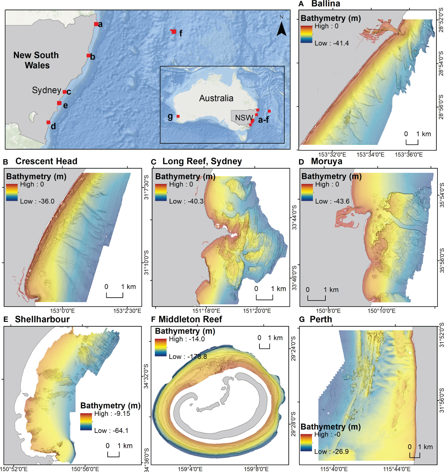
Figure 1 Selected areas of marine lidar data utilised in this study, collected along the New South Wales (NSW) coast (A-D) together with multibeam datasets offshore of NSW (E, F) and marine lidar from Western Australia (G). ESRI basemap.
The toolset settings were further explored on a range of different dataset types (source and resolution) and shelf environments (Table 1). Bathymetric data were sourced to represent different environmental seascapes, data sources (multibeam and marine lidar), data resolutions (2, 5, 10 and 20 m cell size) and data preparation treatments (with and without data smoothing). These datasets include multibeam data collected offshore of Shellharbour, NSW by NSW DPE (Figure 1E), multibeam data collected at Middleton Reef, offshore NSW by the Australian National Environmental Science Program and Geoscience Australia (Figure 1F), and marine lidar collected offshore of Perth, Western Australia (WA) by the WA Department of Transport (Figure 1G). To explore the impact of resolution on tool performance, the 5 m cell size Shellharbour dataset was re-gridded to 10 m and 20 m using the Resample tool in ArcGIS. The toolset was run on bathymetric data with and without the toolset’s smoothing function applied.
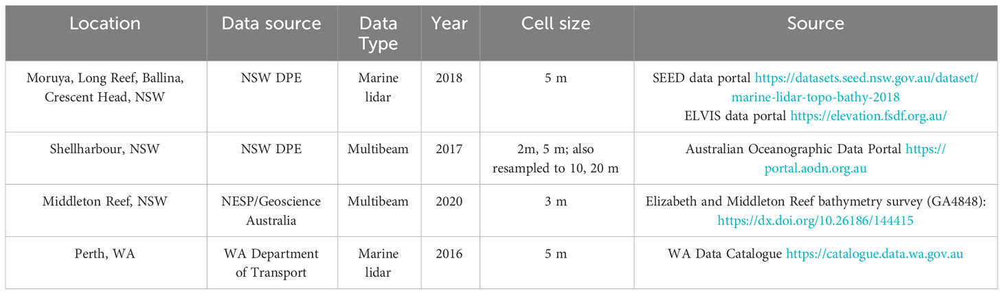
Table 1 Bathymetry data sources.
2.2 Seabed landforms classification toolset
The foundational framework for the seabed classification toolset was developed by Linklater et al. (2019). The methodology presented here further extends this framework into a comprehensive suite of tools, the Seabed Landforms Classification Toolset, which guides the user through the classification process. The toolset utilises a suite of ArcGIS functions in conjunction with functions from existing toolsets including ‘terrain ruggedness’ from Benthic Terrain Modeler (BTM, Walbridge et al., 2018) and ‘slope position’ the Geomorphometry and Gradients Metric Toolbox (GGMT, Evans et al., 2014) and incorporates them into a workflow to classify prominent features within the shelf seascape. Four variables are derived from the bathymetry to characterise the seabed: ruggedness (BTM, Walbridge et al., 2018), slope (Spatial Analyst, Esri), finescale and broadscale Bathymetric Position Index (Slope Position, GGMT, Evans et al., 2014).
Our approach creates a two-part classification, first defining ‘surface elements’ (Table 2) which are the base textural components of the seascape (e.g. rugose outcrop, smooth flat, slope), and subsequently defining ‘seabed landforms’ which aggregate surface elements to identify prominent shelf features (e.g. reef/bank, plain, scarp). Terminology for seabed features (Table 2) has been sourced from established nomenclature within the literature, including the International Hydrographic Organization (IHO) Classification Dictionary (IHO, 2019, the Mareano-Infomar-Maremap and Geoscience Australia (MIM-GA) Morphology Features Glossary (Dove et al., 2020), and Evans (2012) and applied here to a marine environment, with the inclusion of ‘ruggedness’ as a defining variable. Here, ‘landforms’ are largely analogous to the morphology-level scheme presented in Dove et al. (2020), although the approach presented here attempts to provide a single, non-overlapping classification of the entire seascape surface using a more limited set of terms. These terms are intended to capture prominent shelf features and can be modified to suit individual user requirements.
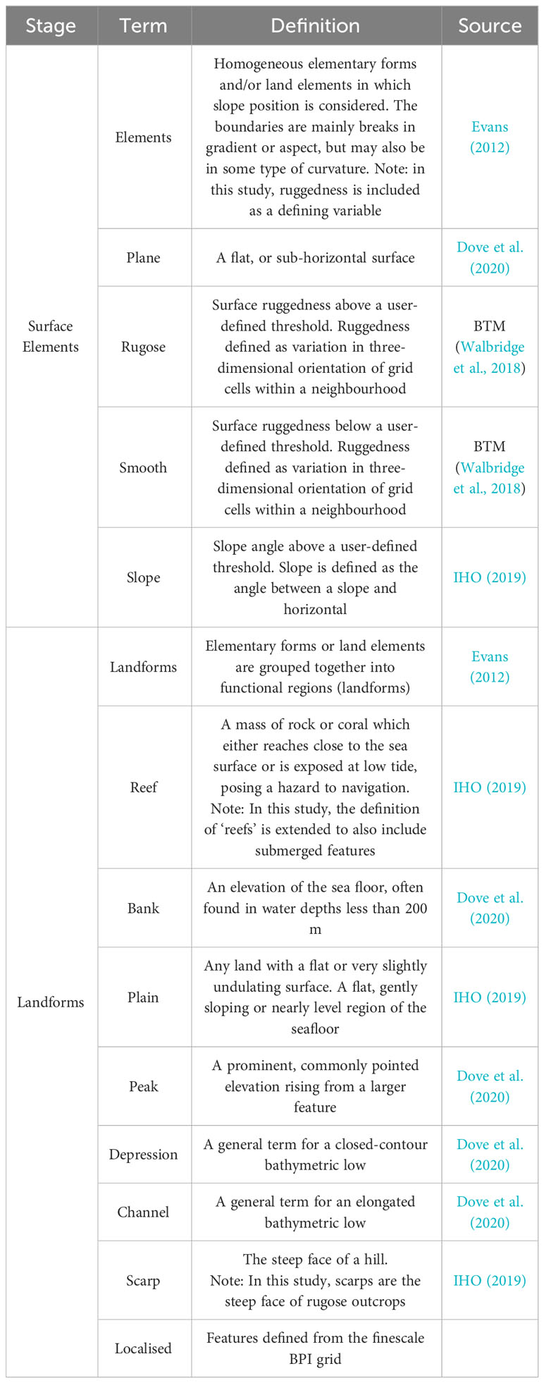
Table 2 Definitions and sources of surface element and landform terms used in classification toolset.
The Seabed Landforms Toolset comprises four main classification stages (Figure 2, Table 3): 1) DEM preparation: this includes steps to prepare the DEM raster for subsequent analysis; 2) Surface Elements classification: this breaks up the surface into key components based on derived variables of ruggedness, slope, finescale and broadscale bathymetric position index (BPI); 3) Landform classification: this translates surface elements into landforms, requiring manual editing and review by the user; 4) Plain classification; this is an optional step to classify plain areas if desired. Each of these classification stages and the tools contained within will be outlined in detail below. The toolset is freely available for download on the NSW Government SEED environmental data portal and GitHub where a user-guide and supporting materials are available, including a web explainer (Linklater et al., 2023). Procedures are introduced to identify polygons within rugose outcrops, reduce potential noise, classify low-relief landforms within plain areas (e.g. bedforms), perform manual editing, as well as a broad range of additional functionality, as outlined below.
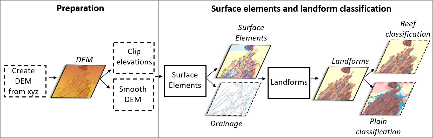
Figure 2 Workflow diagram showing the relationship of the key classification stages and resulting outputs. Dashed outline indicates optional processing steps and outputs. Square = tool; parallelogram = dataset.
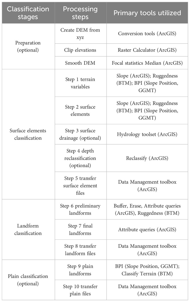
Table 3 Summary of the classification stages within the Seabed Landforms Classification Toolset, and the processing steps and primary tools associated within each classification stage.
2.2.1 DEM preparation
Functionality is included to assist users in preparing the DEM for analysis. Tools are included to grid a DEM from XYZ input data, clip data to set elevation range, and smooth the DEM, as required for the individual dataset. The toolset has been designed for open coast shelf settings and has not been tested for land or estuarine settings, or data that extends beyond the shelf break.
The smoothing function performs a median filter using the ‘Focal Statistics’ tool within ArcGIS (Esri, 2021), where users can input the number of smoothing iterations. Median filters were determined to be the most effective as they do not include the extremities of values as would occur with a mean calculation (Linklater et al., 2018). Where speckled noise artefacts occur within the dataset, smoothing is effective at reducing this noise and improving the distinction between rugose outcrops and surrounding plains (Supplementary Figure 1).
2.2.2 Surface element classification
The surface elements classification breaks up the seascape into components based on slope (ArcGIS Spatial Analyst, (Esri, 2021), ruggedness (Benthic Terrain Modeler, BTM, Walbridge et al., 2018), and bathymetric position index ‘BPI’ (Slope Position, Geomorphometry and Gradients Metric Toolbox, GGMT (Evans et al., 2014). The resultant classification defines slopes, and rugose or smooth highs, lows or planes occurring at finescale or broadscale extents within the seascape. This further develops the framework presented in Linklater et al. (2019) into a sequence of GIS tools (Table 3).
The thresholds to define the surface elements are user-defined, with settings dependent on the resolution and extent of bathymetric data, as well as features of interest. Default settings of the tools are presented in Table 4. These were developed for data inputs of 5 m cell size with three smoothing iterations. The default settings were chosen as they are suitable for the NSW statewide marine lidar and multibeam datasets, but are also representative of common input bathymetry datasets, which will often require smoothing. The 5 m cell size is a mid-level resolution for bathymetric datasets and an appropriate resolution for reef mapping at comparable scales (e.g. Lucieer et al., 2016). These thresholds have been modified where required for each of the datasets presented.
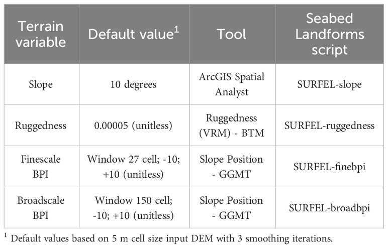
Table 4 Terrain variables with default values used in classification toolset, key tool utilised and associated script within toolbox.
The surface elements classification outputs 11 classes characterising the surface based on superimposed reclassifications of ruggedness (rugose or smooth), broadscale and finescale BPI (finescale or broadscale high, low or flat) and slope (high slope) variables (Supplementary Table 2). Areas defined by the user as ‘slope’ (for example, all areas greater than 10 degrees with a user-defined threshold of 10) overrides all other classes. The remaining area of the surface, which are slope areas below the user-defined threshold, are classified based on ruggedness and BPI. These 11 classes are in turn aggregated into 7 classes to create a summarised surface elements layer including: rugose outcrop, rugose outcrop peak, smooth outcrop, smooth low, rugose low, smooth flat, and slope (Supplementary Table 2). The surface elements layer represents the full suite of component elements, while the summarised surface elements offer a more practicable layer for users to interpret features.
Within the surface elements classification toolset are two optional functions to generate a theoretical surface drainage grid and a depth reclassification polygon. The surface drainage classification represents theoretical surface drainage and is developed from the steps outlined in Linklater et al. (2019). This tool utilises the Hydrology toolbox in ArcGIS (Esri, 2021) to calculate flow direction and accumulation, with the resultant output of flow drainage log-transformed and clipped to 100 m3 to show dominant drainage pathways. The drainage calculation here is not intended as a precise measure of surface volume and accumulation. The calculation is instead intended as a guide to assist the user in identifying paleochannels within the seascape, as the drainage surface may represent active bottom current or relict drainage across the surface during periods where lower sea level may have exposed the shelf.
The depth reclassification is also an optional function, which is analogous to the ArcGIS ‘contour’ tool, that users can use to generate a depth-stratified polygon based on a user-defined interval. This layer is not utilised elsewhere within the classification but is a complementary layer that may be used for assisting analysis and interpretation. For example, depth intervals may be used to stratify the output landforms classification to calculate the proportion of features in each depth interval.
2.2.3 Landform classification
Seabed landforms are defined from the classified surface elements, where multiple surface element classes may be ultimately grouped to form a landform (Supplementary Table 2, Table 2). Landforms represent key features of the seascape, including “reefs/banks”, “peaks”, “plains”, “scarps”, “depressions and channels”. “Reef/bank” definitions were sourced from the International Hydrographic Organization Dictionary (IHO, 2019), whereby “reefs” represent rocky or biogenic outcrops and “banks” represent soft-sediment outcrops. Using the semi-automated classification approach presented, inferred hard substrate “reefs” and inferred soft sediment “banks” are indistinguishable based on the ruggedness measure where soft sediment expression is sufficiently raised and complex or hard substrate is sufficiently smoothed. “Peaks” represent a pointed elevation rising from a larger feature (Dove et al., 2020), and “depressions” and “channels” are closed contour or elongated bathymetric lows, respectively (Dove et al., 2020). “Plains” are horizontal or near-horizontal areas (IHO, 2019), characterised by consistently smooth areas. “Scarps” are steep areas (IHO, 2019) occurring on rugose outcrops occurring on rugose outcrops. Thresholds to define these features are user-defined within the classification toolset. The terms selected were chosen to capture the most prominent features within a continental or island shelf setting, and do not represent the only landforms that may occur within a seascape. The aggregate term “reef/bank” provides a useful conglomerate term for outcropping rugose features of varied shapes, sizes, and inferred composition.
The procedures to identify landforms from surface elements are semi-automated, with the user required to enter classification thresholds and perform manual editing tasks at several stages. This inclusion of manual inputs provides flexibility within the toolset to edit and customise the classification output. Key stages of the landform classification procedure include: 1) identifying polygons within rugose outcrops; 2) creating preliminary landform labels; 3) manual editing of preliminary landform layer; 4) eliminating ‘noise’ polygons; and 5) finalising landform labels.
If desired, the user may seek to manually separate “reefs” from banks and other plain features (Figure 2). Although the landform classification isn’t intended to explicitly map substrate, inferred hard-substrate ‘reef’ areas could be distinguished from inferred soft-substrate ‘banks’ by the user using expert knowledge and manual editing, with examples of these optional edits presented in this study. Further separation of the classes defined in the toolset, including “reef/bank” outcrops and “depressions and channels” into more detailed morphological terms or regionally specific terms is encouraged where desired by the user.
2.2.4 Plain classification
The plain classification toolset can be utilised where the user desires a separate reef and plain classification. Once the plain polygon area has been determined from the landform classification procedure, the DEM extracted over these areas can be used to generate a detailed classification of prominent inferred soft-sediment features within the plain.
Plain landforms are defined using finescale and broadscale BPI, creating classes including: plain high, plain low, localised high, localised low and plain flat. The plain classification is designed to be performed on areas of DEM data extracted from the classified ‘plain’ features (i.e., excluding other landform areas).
This classification is an optional procedure which intends to capture additional detail across the plain area for users focused on the inferred sedimentary environment. The plain classification is categorised as an ‘optional’ step as it is not required to be run in sequence for other subsequent scripts to operate. It is, however, an important component of the classification approach, and is recommended to be performed in areas of complex soft sediment morphology. Vast areas of continental and island shelf systems are characterised by plain landscapes, and the plain classification method can extract fine and broadscale features within this environment for the user to interpret.
Feature terms utilised in the plain classification (e.g. localised high) are intentionally generic so the user can apply or describe features based on site specific interpretations. “Low” features in the plain classification are similar to the “depressions and channels” features in the main landform classification in that they are both defined using BPI. However, “depressions and channels” in the main landform classification are characterised as occurring within rugose outcrops, and broadscale and finescale low classes are combined. In the plain classification, finescale (localised) and broadscale high and low features are retained, and ruggedness and slope variables are removed as they were determined as less effective at capturing the detailed surface variation of generally smoother plain environments.
Examples of the plain classification are provided for offshore of Ballina and Crescent Head, NSW using the statewide marine lidar 2018 dataset.
2.3 Application of toolset to varied data scenarios
To further assess the performance of the Seabed Landforms Classification Toolset and determine suitable settings, the classification approach was applied to a range of varied bathymetric data scenarios including data representing different: 1) data sources (multibeam and marine lidar); 2) environmental seascapes; 3) data resolutions (2, 5, 10 and 20 m cell size), and: 4) data preparation treatments (with and without data smoothing). Data preparation methods and tool settings were adjusted to assess the suitability of the tools to diverse environmental seascapes across varied data scenarios.
Firstly, the toolset was explored using datasets sourced from different remote sensing technologies including multibeam and marine lidar which were acquired using varied acquisition and processing systems, sensors and vessels. Selected areas from the NSW marine lidar were examined (Moruya, Long Reef, Ballina, Crescent Head), together with multibeam data collected at Shellharbour by DPE, marine lidar data collected offshore of Perth, Western Australia (WA) by WA Department of Transport (Western Australia Department of Transport, 2017), and multibeam data collected around Middleton Reef by the National Environmental Science Program (NESP) with Geoscience Australia (Figure 1, Carroll et al., 2021). The variation in input data sources allows for an exploration of settings relating to noise correction, particularly regarding the level of smoothing for noise artefacts.
Secondly, data collected from different environmental seascapes were utilised to explore the effectiveness of the tools at capturing a variety of outcropping shelf features across diverse environments (see Figure 1). Areas along the NSW coast and offshore, including Moruya, Long Reef and Shellharbour provide examples of rocky reefs outcropping from a surrounding sediment plain (Kinsela et al., 2022). The sediment plain is further examined with Ballina and Crescent Head marine lidar data classified using the optional plain classification functionality. The Shellharbour dataset represents similar features to those observed at Moruya and Long Reef from the statewide marine lidar, though is instead captured with a multibeam sensor and extends to deeper waters down to 64 m depth. Offshore of Perth, WA, submerged landforms may represent drowned Quaternary fossilised barrier and dune sequences, as described in this setting by Brooke et al. (2014). The submerged ridge and mound features surrounding the atoll-like Middleton Reef are of undetermined origins, though appear similar in morphology to drowned fossils reefs observed on the nearby Lord Howe Island shelf, which occur further south in the island-reef chain offshore of NSW (Carroll et al., 2021).
Furthermore, the adjustment of tool settings in relation to input resolution was examined. The highest resolution dataset was represented by the Shellharbour data (2 m), and this data was re-gridded (down-sampled) to 5, 10 and 20 m to explore how input settings change with resolutions. Resolutions beyond 20 m were not explored as the toolset is designed for higher-resolution data that is typically collected in nearshore and shelf settings. Data from the other case study areas ranged from 3 to 5 m cell size (Table 5).
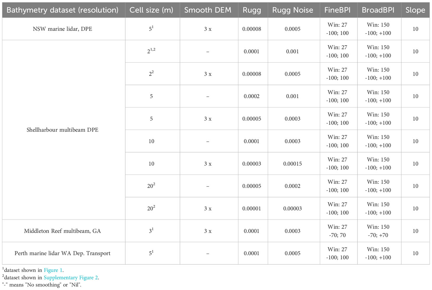
Table 5 Classification settings for NSW marine lidar selected areas (Moruya, Long Reef, Crescent Head, Ballina), Shellharbour multibeam data (NSW Department of Planning and Environment, DPE), Middleton Reef multibeam data (Geoscience Australia, GA) and Perth marine lidar (Western Australia Department of Transport).
Finally, different data treatments to the input bathymetric data were applied to explore the effect of smoothing. The toolset was applied to each of the Shellharbour datasets (cell size 2, 5, 10 and 20 m) without smoothing, and with the default level of smoothing of three iterations of a median filter. Examining optimal settings for data at a range of resolutions, with and without smoothing applied, provides a guide for users when exploring their own datasets. For the remaining datasets, the most appropriate smoothing treatment was applied to optimise the output classification.
3 Results
3.1 DEM preparation
The NSW marine lidar data was clipped to 0 m elevation (Australian Height Datum) to remove land features, and three iterations of data smoothing was applied due to the increase in speckled noise in deeper waters. Increased noise in turbid or deeper waters is common in marine lidar datasets due to the reduced capacity for laser penetration which results in fewer data points captured (Quadros, 2013). Three iterations of smoothing with a median filter using the ‘Smooth DEM’ tool were shown to improve the noise within the DEM and derived variables (Supplementary Figure 1).
3.2 Surface element classification
The example areas from the marine lidar datasets were classified using the same threshold settings due to the similarities in scale and expression of features, data quality and input resolution (5 m cell size, Table 5). The default ruggedness value of 0.00005 was slightly adjusted to 0.00008, with all other default settings for BPI and slope remaining. The default settings were developed to apply to the entire statewide marine lidar dataset and therefore represent generic settings, however the value has been slightly adjusted in this case to best exemplify reef extent in these areas. In the example of Moruya data (Figure 3), ruggedness effectively captures the prominent rugose outcrop and channels within the outcropping surface. The drainage surface highlights narrow channels on the outcrop surface, which are largely captured as ‘low’ smooth or rugose features at fine and broad scales within the surface elements and summarised surface elements classifications (Figure 4). The uppermost parts of the outcropping rugose feature are captured as ‘peaks’, with limited slope areas on the edges of the outcrop due to the relatively low-profile nature of the rugose outcrop (~ 10 m in relief at peak of structure from the surrounding plain).
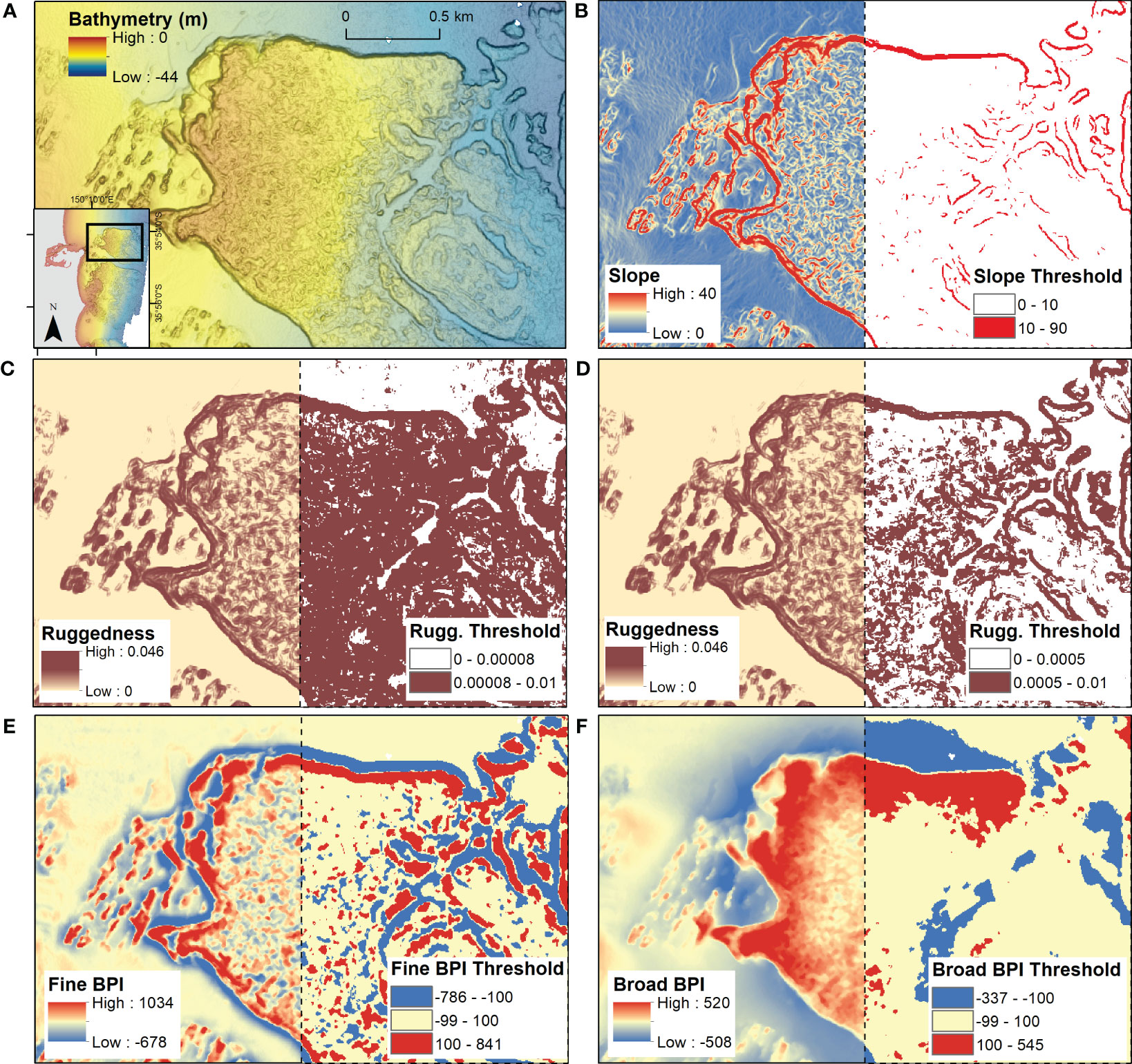
Figure 3 Input terrain variables and reclassification thresholds for Moruya, NSW lidar data. Continuous data shown on LHS, with reclassified data shown on RHS; (A) lidar bathymetry; (B) slope as continuous data (LHS) and reclassified at 10 degree threshold (RHS); (C) ruggedness as continuous data (LHS) and reclassified at 0.00008 (RHS); (D) ruggedness as continuous data (LHS) and reclassified at 0.0005 (RHS); (E) finescale BPI as continuous data (LHS) and reclassified at -100 and 100 (RHS); and (F) broadscale BPI as continuous data (LHS) and reclassified at -100 and 100 (RHS).
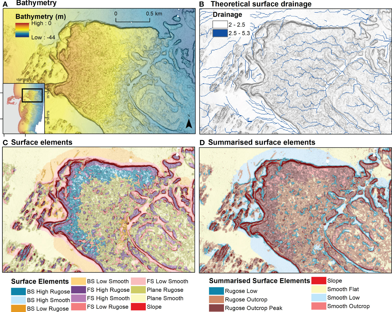
Figure 4 Surface element and drainage classifications for Moruya, NSW lidar; (A) lidar bathymetry; (B) theoretical surface drainage showing dominant pathways; (C) surface elements classification (BS, broadscale; FS, finescale); (D) summarised surface elements classification with grouped classes for ease of use.
3.3 Landform classification
The landform classification carries the summarised surface element terms across to form preliminary landform terms, to be reviewed and edited by the user. Preliminary landform labels for the Moruya and Long Reef example areas are shown in Figures 5, 6 respectively, with required and optional landform edits indicated.
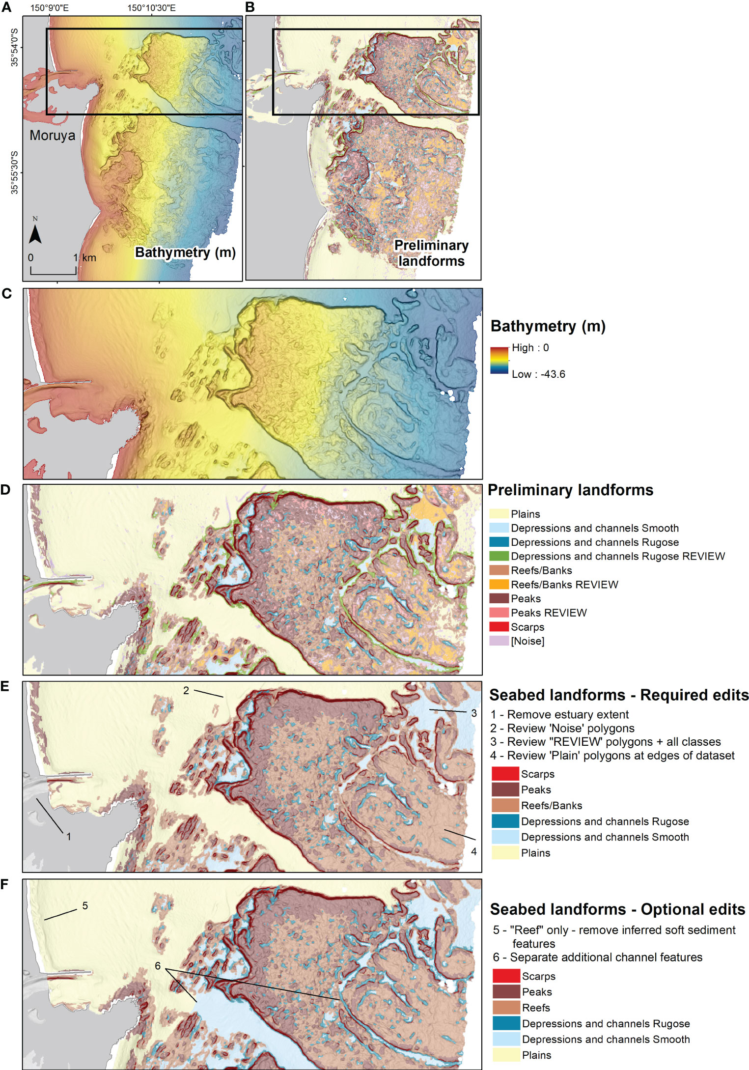
Figure 5 Landforms classification for Moruya, NSW lidar; (A) lidar bathymetry and (B) preliminary landforms; (C) lidar bathymetry of example classification area; (D) preliminary landforms layer as output from classification toolset, requiring manual review and editing; (E) seabed landform classification finalised with required level of manual editing and review; (F) seabed landform classification finalised with additional optional level of manual editing and review. Small polygons eliminated <100 m2.
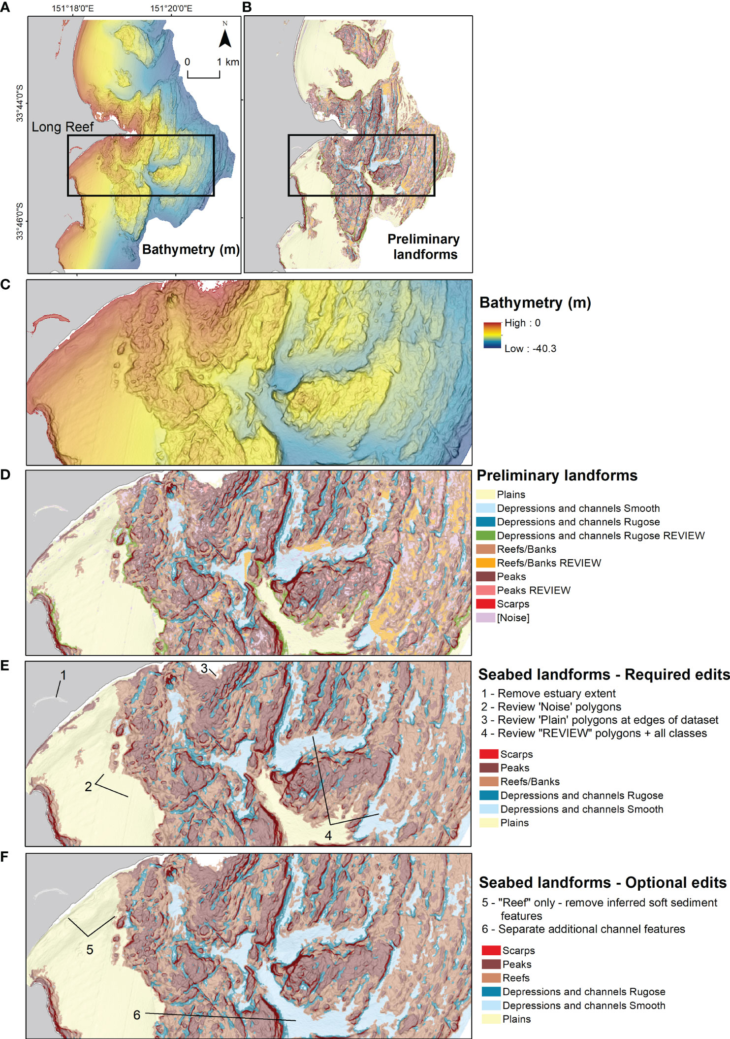
Figure 6 Landforms classification for Long Reef, NSW lidar; (A) lidar bathymetry and (B) preliminary landforms; (C) lidar bathymetry of example classification area; (D) preliminary landforms layer as output from classification toolset, requiring manual review and editing; (E) seabed landform classification finalised with required level of manual editing and review; (F) seabed landform classification finalised with additional optional level of manual editing and review. Small polygons eliminated <100 m2.
A minimum level of manual reviewing and editing is required, including removing estuary extents (if applicable), and reviewing all class labels, ‘noise’ polygons, and polygons at the edges of the dataset. Polygons which form part of the reef/bank structure may be classed as ‘plains’ where they occur at the boundary of the dataset, as the procedures to identify smooth, flat areas within rugose outcrops require the smooth polygons to be wholly surrounded by a rugose outcrop. Therefore, edges of the dataset must be reviewed to ensure correct attribution of landform label, in addition to all classes which must be reviewed and edited by the user to ensure the classification meets the interpreted feature expression.
Optional manual editing may be performed by the user where additional or modified classes are desired. ‘Reef’ features (inferred hard substrate) may be separated from ‘banks’ (inferred soft substrate), where deeper knowledge of the environment is available. Examples of such editing processes are provided in Figures 5, 6. In these examples, reefs/banks which occur as shore-parallel features (surf zone bars) along the nearshore seabed are inferred as soft sediment banks and may therefore be removed by the user if a reef-only classification is desired. Additional channel features may also be included, which involves cutting and relabeling polygons (‘plain’ polygons or ‘depressions and channels rugose REVIEW’ polygons) to capture channels which may occur between or within reef/bank outcrops. For example, optional editing undertaken for the Moruya dataset captured additional channel features including the central channel which divides the two prominent reef outcrops. The resulting classification is flexible to user requirements, and users may further perform optional manual edits and modify landform terminology as desired.
3.4 Plain classification
In the examples of the plain classification shown for Ballina and Crescent Head marine lidar data, localised and broadscale high and low features are captured (Figure 7). In these examples, the reef outcrops have been separated from the surrounding plain, inferred as soft-sediment areas. “High” features which may have been originally captured as reefs/banks in the main landform classification have been relabelled as part of the plain surface. With the ruggedness and slope variables excluded from the plain classification, features within the plain are characterised by finescale and broadscale BPI which captures detailed surface morphology of these inferred sedimentary environments. The BPI-based plain classification captures complex bedforms that have been interpreted as finer scale sandwaves superimposed on larger sand waves and sand ridges (Kinsela et al., 2023). Scour channels, scour depressions and sand ridges are also captured as localised high and low features.
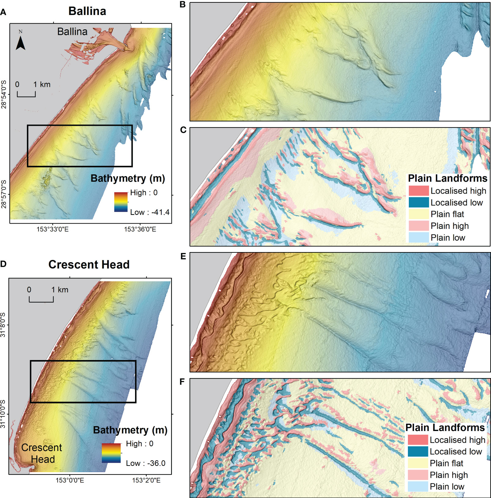
Figure 7 Plain classification for Ballina and Crescent Head, NSW marine lidar; (A) lidar bathymetry for Ballina with (B) close-up bathymetry and (C) plain classification; (D) lidar bathymetry for Crescent Head with (E) close-up bathymetry and (F) plain classification. Eliminated small polygons <800 m2.
3.5 Application of toolset to varied data scenarios
The application of the Seabed Landforms Classification Toolset was examined using input data from a range of scenarios including acquisition sources, seascape environments, resolutions and data preparation techniques. Input settings were adjusted to each dataset to optimise the resulting classification (Table 5), which can guide users when examining their individual datasets.
Ruggedness was the key variable which required alteration for each scenario, while slope and BPI variables were able to remain at the default settings. All preliminary landform output layers were reviewed and manually edited with required edits, including reviewing noise polygons, class labels, and polygons at the edges of the dataset, as discussed in Section 3.3. An effective classification of seabed landforms with varied morphologies and expressions was achieved across all areas presented (Figure 8). More extensive manual editing was undertaken for the Moruya, Long Reef, Ballina and Crescent Head where reefs were separated, however minimal manual editing was required to generate the final landforms classification for the remaining areas examined. Across all datasets, the resulting classifications captured both networks of larger reef/bank outcropping features, as well as smaller, isolated patchy reef/bank outcrops and output an effective classification of prominent features.
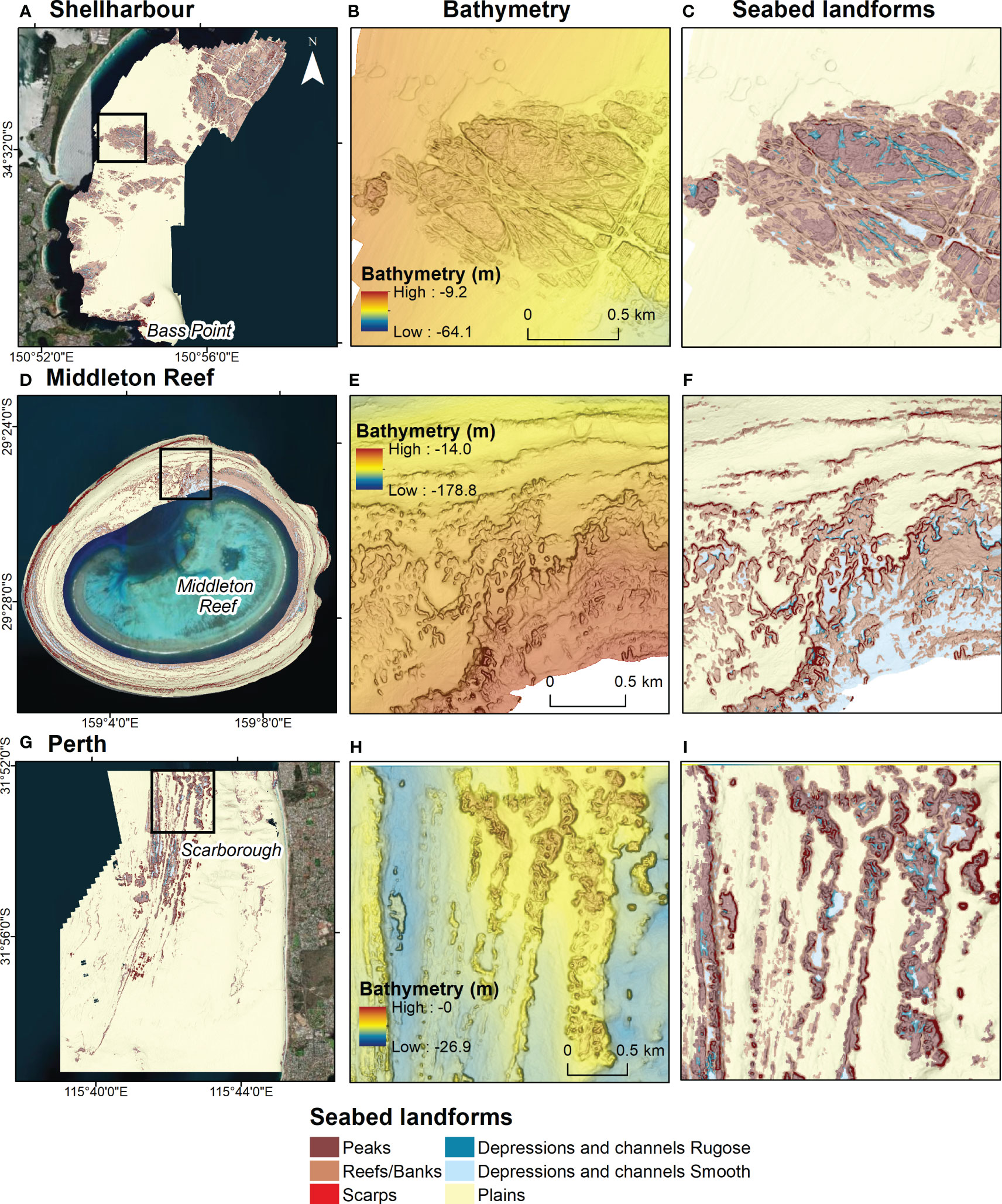
Figure 8 Applications of seabed classification to; (A) Shellharbour multibeam landforms classification; with example area (B) Multibeam bathymetry data; and (C) classified seabed landforms with required edits; (D) Middleton Reef landforms classification; with example area (E) Multibeam bathymetry data; and (F) classified seabed landforms with required edits; (G) Perth marine lidar data; with example area (H) lidar bathymetry data; and (I) classified seabed landforms with required edits. Basemaps provided by Esri.
The classification tools effectively translated to varied environments, all occurring within a continental or island shelf setting. In Shellharbour, the method is shown to capture the full extent of broad reef outcrops, which have a platform-type morphology. Channelling is detected within the reef outcrop surface, which could be further incorporated with additional optional manual editing (e.g. Figures 5, 6). Classified “reefs/banks” have reliefs ranging 3 to 6 m from the surrounding plain surface. At Middleton Reef, both narrow and broad ridge-like outcropping features are captured (with reliefs up to 8 m) as well as small, patchy outcrops (1 to 6 m in relief). Broader depressions and channels occur as distinct from the outcropping reef/bank feature. “Reefs/banks” features were further differentiated into ridges and mounds in subsequent analysis of the classified dataset by Carroll et al. (2021), where landform terms were aligned to Dove et al. (2020), which outlines a more comprehensive suite of seabed morphological feature terms. The ability to easily adapt the output classification terms as needed demonstrates the flexibility of output classification to meet varied user requirements. In the resulting classification of the Perth dataset, parallel (sub-parallel) elongate ridge-like reefs/banks are effectively captured, with outcrops ranging 1 to 4 m in relief. Using the settings applied here, broader banks inshore (Figure 8G) are less effectively captured to their full extent, and a lower ruggedness setting could be employed to capture a greater extent of these features if desired.
In terms of implementation of the toolset with different data acquisition sources, the main consideration is whether or not to apply smoothing. Typically, bathymetry data sourced from marine lidar may require additional smoothing to reduce noise artefacts (e.g. Supplementary Figure 1). Different smoothing treatments were applied to the multibeam data, with smoothing applied to Middleton Reef dataset and no smoothing applied to the Shellharbour dataset. This resulted in examples with and without smoothing for marine lidar data sources (NSW examples and Perth), as well as multibeam sources (Shellharbour and Middleton Reef).
The application of smoothing, regardless of input source data, alters the ruggedness threshold required. With increased iterations of smoothing, it was shown that the ruggedness threshold needs to be lowered accordingly (Table 5). For the 2 m Shellharbour DEM, a ruggedness threshold without smoothing of 0.0001 is lowered to 0.00008 when smoothed with three iterations. This is due to the nature of the smoothing calculation, which reduces the ‘roughness’ of the surface and therefore the ruggedness value needs to be lowered with each smoothing iteration accordingly. In the Shellharbour example (Supplementary Figure 2), smoothing may not be preferred where reef outcrops are the focus output (i.e. if the user ultimately wants to separate inferred reef from inferred banks). Excess smoothing can reduce the effectiveness of the ruggedness threshold at capturing reef edge, and can introduce more inferred soft-sediment banks, as can be seen in the smoothing of 20 m dataset (Supplementary Figure 2F).
Input resolution was explored using the Shellharbour multibeam re-gridded from 2 m to 5, 10 and 20 m. As the input cell size coarsened, the ruggedness value was lowered to capture a similar extent of rugose outcrops (Supplementary Figure 2). For the 2 m DEM, a ruggedness threshold of 0.00008 was determined suitable, decreasing to 0.00001 for the 20 m DEM. In this example, input cell size does not seem to alter the BPI window scales and thresholds outside the default tool settings (Table 5). While BPI thresholds will vary based on the spatial extent of data, distribution of depths within the data, and occurrence of sharp gradient shifts, overall, the settings for BPI appear largely robust to changing input resolutions for an individual survey.
Overall, it was found ruggedness is the most critical variable to alter with varied input datasets and preparation treatments as the threshold value has the greatest impact on the extent of reef/banks captured. BPI and slope can also be adjusted as needed, though remained the same across the areas presented due to the similarities in the magnitude of features mapped in the examples presented.
4 Discussion
The new classification procedure we have presented as part of the Seabed Landforms Classification Toolset provides users with a whole-landscape classification of prominent shelf landform features. The semi-automated nature of the procedure results in improved efficiency when undertaking seabed classifications, which can be applied more readily to largescale datasets. A number of example areas have been presented to demonstrate tool performance, with notable seabed features shown to be effectively captured across a diverse range of data input scenarios, including varied acquisition sources, environments, resolutions and data preparation settings.
4.1 Effectiveness of classification approach
The use of the ruggedness variable is central to the classification approach presented, forming the basis of the delineation of reef/bank outcrops. Reef/bank features, as presented here, are an aggregate landform term which can encapsulate shelf features referred to in other terms such as platforms, ridges, hills and mounds (e.g. Dove et al., 2020). Ruggedness has shown to be a useful measure for seascape characterisation (Johnson et al., 2017; Linklater et al., 2019; De Oliveira et al., 2020) and this study lends further support to its application in identifying the boundaries of reef outcrops. The introduction of the noise correction procedures through the toolset further enhances the application of ruggedness, as noisiness in the data, which may have previously limited the use of ruggedness in identifying reefs, can be largely addressed. When integrated together with slope, finescale and broadscale BPI, this study has shown the successful characterisation of the key components of a seascape across a range of example areas. The outcropping structures are delineated into a suite of landform terms, which adds meaningful delineations of the surface structure into classes such as scarps and peaks, which can be used for subsequent interpretations and analysis of the dataset. While a more detailed suite of morphological terms may be applied through methods or classification schemes outlined in other studies (e.g. Dove et al., 2020), the more limited suite of terms employed in this study aims to aggregate key features into a practicable set of terms which can be used to classify the entire seascape surface.
With concerted efforts to map seafloor bathymetry at regional (e.g. SeaBed NSW), national (e.g. Australian HydroScheme Industry Partnership Program, Houston, 2020) and global (e.g. SeaBed 2030, Mayer et al., 2018) scales, the semi-automated toolset holds great potential for extracting key landform features. The morphology-level characterisation of the seascape into ‘landforms’ breaks up the surface into components based on surface variation, and therefore does not require ground-truthing validation data as would be required for geomorphology, substrate or benthic habitat maps. It is therefore an ideal first product from bathymetry data collected where ground-truthing data may not be present. Where ground-truthing data is available, the delineated boundaries of landform features may be validated, and the landform classification may be integrated together with substrate or biota classifications to generate maps of seabed geomorphology or benthic habitat (e.g. Linklater et al., 2019). Detailed seabed landform classifications can be applied to wide-scale datasets, such as the SeaBed NSW program, which can in turn contribute towards consolidated seabed mapping products at national scales (e.g. SeaMap Australia, Lucieer et al., 2019).
4.2 Semi-automated approach
The classification workflow is broken down into a set of 10 practical steps for users to apply and review. The use of the toolset will significantly reduce the time required for manual editing, particularly of large bathymetry datasets, and applies a consistent scheme which is less subjective than manual digitisation approaches. The incorporation of a manual component of reviewing and editing features in order to progress to the final landforms classification stage provides this opportunity for expert review, which is necessary to ensure the feature boundaries and terms reflect the users requirement. The semi-automated nature of the methods balances the need for automation due to ever-increasingly high volumes of data, together with the importance of expert interpretation.
Within the seabed mapping community, there is a growing effort toward automation (Lecours et al., 2018) an identified interest in adopting semi-automated classification procedures from users who do not currently employ them in their current workflows (Dove et al., 2019). Available skills, transparent workflows and inconsistencies in standards for terms and procedures were identified as barriers to adopting semi-automated workflows (Dove et al., 2019). These tools are designed to address these barriers of seabed classifications for new users. The design of these tools as an ArcGIS toolbox assists in increasing the accessibility of the tools to the seabed mapping community, utilising ruggedness from the BTM toolbox (Walbridge et al., 2018) as well as functionality within Geomorphometry and Gradients Metrics Toolbox (GGMT), (Evans et al., 2014). Ruggedness is integrated into the workflow to optimise delineations of reef outcrops, and additional steps are incorporated to address and minimise noise and identify the full extent of reef outcrops. Standardised seabed morphology terms (IHO, 2019; Dove et al., 2020) are incorporated, and Python scripts associated with the ArcGIS toolbox are accessible to users, providing a completely transparent methodology.
The toolset presented contributes towards a standardised methodology and symbology for geomorphometric and geomorphological analysis, which has been identified as a key area of focus for the marine geomorphometry community (Lecours et al., 2016). The tools are designed to be accessible to a broad range of GIS users, enabling a wider adoption of marine geomorphometric analysis into the workflows of users interested in performing seabed classifications.
4.3 Targeting classification approach to varied scenarios
A range of bathymetry datasets were presented to exemplify how the tools can be applied across varied shelf environments and data input scenarios, with the classification approach shown to translate effectively across all scenarios with adjustments to input settings. Bedrock rocky reef outcrops along the NSW inner and mid shelf (i.e. Moruya, Long Reef, Shellharbour, Figures 5, 6, 8) were successfully captured by the classification toolset, as well as dynamic soft-sediment bedforms of the northern NSW coast (Ballina, Crescent Head, Figure 7). It can also be effectively applied to submerged ridges offshore of Perth, WA, and submerged features on the shelf surrounding Middleton Reef (Figure 8). In the case of the Middleton Reef landform classification, further analyses undertaken by Carroll et al. (2021) modified the output “reef/bank” label to “mounds/ridges”, demonstrating the ability of the landform terms to be customised to individual user-needs.
The plain classification approach has been effectively applied to capture detailed bedforms within the plain landscape, with examples provided in this study and Kinsela et al. (2023). Classified plain features offshore of Ballina, NSW, aided in the interpretation of sedimentary features by Kinsela et al. (2023) and assisted in assessing the depositional or erosional origins and interactions of features.
The classification toolset intentionally applies a more limited suite of terms to the final classified landforms to aid simplicity for end-user interpretation. However, additional analysis such as depth reclassification into depth intervals or slope reclassification into gentle, moderate and steep slopes, for example, is encouraged. Such analyses are complementary to the classification and can be integrated into the final landforms output where desired by the user.
With adjustments to input settings and data smoothing (Table 5), the classification approach was shown to perform well with data from different acquisition sources (marine lidar and multibeam) and resolutions (2, 5, 10 and 20 m cell size). Ruggedness is the main variable that requires adjustment of the threshold value, with particular attention needed when smoothing the DEM. As resolution coarsens or as the level of smoothing iterations increase, the ruggedness threshold needs to be lowered accordingly. While each dataset needs to be assessed individually, generally marine lidar datasets or satellite-derived bathymetry may be more likely to require smoothing due to speckled noise artefacts that can occur, particularly in deeper and turbid waters.
Exploration of scale is an important factor in seabed analysis (Lecours et al., 2016; Misiuk et al., 2021), and the toolbox presented enables users to adjust scale through the finescale and broadscale BPI variables to suit features of interest/environment. The transparency of the toolset allows for explicit comparison of the varied outputs when altering scale and resolution input settings, as well as other factors which may influence the output classification (e.g. data smoothing).
The toolset presented was developed for open coast, nearshore and shelf seabed data and has not been explored outside these environments. Data resolutions were tested up to 20 m with source depth data equivalent to 20 m point spacing or less. Tool performance on source point data greater than 20 m spacing or interpolated datasets have not been tested. Procedures to reduce noise were incorporated into the classification, which can reduce noise artefacts where speckled noise is present. Such techniques may be less effective where more pronounced noise artefacts occur, such as nadir or edge effects, or roll and heave artefacts which are sufficiently large to be captured by the user-defined ruggedness noise threshold.
All scripts are available within the Seabed Landforms Classification Toolbox should the user require to view or modify the scripts to target individual user requirements.
4.4 Standardising seabed classifications and terminology
Recent developments have focused on creating a standardised approach to classifying the marine seascape, including shelf settings, with Mareano-Infomar-Maremap and Geoscience Australia (MIM-GA) drafting an international framework for marine feature terms (Dove et al., 2020; Nanson et al., 2023). This classification extends the international and national schemes which have attempted to create a unified set of terms that are consistently applied to shelf environments (Greene et al., 1999; Galparsoro et al., 2012; Johnson et al., 2017; IHO, 2019). The suite of terms developed by Dove et al. (2020) provides a comprehensive suite of morphological terms and selected terms applied here, together with terms from the International Hydrographic Organization (IHO, 2019), where appropriate.
Aggregate terms, such as ‘reefs/banks’ and ‘depressions and channels’, were applied here to simplify the classification process and output for users. The challenge with the reef outcrops described along the NSW coast in the lidar and multibeam is that they exhibit a diverse range of shapes and configurations, often as amorphous reef outcrops. Furthermore, the scope of coverage in the case of reefs mapped by the NSW DPE SeaBed NSW lidar and multibeam mapping program, means that aggregate terms are helpful due to the scale of data to be classified. This approach attempts to provide a classification suited for most types of data, where users are attempting to capture the dominant visible features within a seascape, and has applied terms that are commonly used and interpretable by users while also meeting definitions and criteria within the literature and international standards (IHO, 2019; Dove et al., 2020). The polygons defined in this process can be further analysed to separate reef patches and other features into more specific terms, such as hills, mounds, ridges and platforms (e.g. Dove et al., 2020; Carroll et al., 2021). Additional optional manual editing can also be undertaken to further separate depressions and channels into more specific features such as sinuous or straight channels, troughs, crevices, as per Linklater et al. (2019). Overall, the classification approach presented is intended to strike a balance between automation and expert interpretation, and furthermore balances the need for standardised methods with flexibility of individual user-requirements. This toolset contributes toward the standardisation of seabed classification and marine geomorphometric methods and encourages accessibility of methods to new users interested in introducing semi-automated workflows into seabed classification approaches.
5 Conclusions
The Seabed Landforms Classification Toolset offers a semi-automated and effective procedure designed to classify prominent shelf features on continental and island shelf settings. The classification approach generates a ‘landform’ classification of the entire seascape, defining polygon boundaries for morphological features including reefs/banks, peaks, scarps, plains, and depressions and channels. The terms and classified output are customisable to the user’s needs, and the method incorporates manual review and editing to balance the benefits of automation with the benefits of expert interpretation. Optional functionality is included to classify the detailed bedforms of plain areas, as well as additional functions to prepare the digital elevation model and assist in seascape classification and interpretation. The toolset is designed to be accessible to users within the seabed mapping community, offering a user-friendly approach to generate a detailed shelf seabed feature classification which can provide critical foundational information for marine and coastal management, research and planning.
Data availability statement
The datasets presented in this study can be found in online repositories. The names of the repository/repositories and accession number(s) can be found below: The Seabed Landforms Classification Toolbox and associated resources can be downloaded from the NSW Government SEED environmental data portal: https://datasets.seed.nsw.gov.au/dataset/seabed-landforms-classification-toolset and GitHub: https://github.com/LinklaterM/Seabed-Landforms-Classification-Toolset. NSW Department of Planning and Environment statewide marine lidar is available from the SEED data portal: https://datasets.seed.nsw.gov.au/dataset/marine-lidar-topo-bathy-2018 and ELVIS data portal: https://elevation.fsdf.org.au/. NSW Department of Planning and Environment Wollongong and Shellharbour multibeam echosounder data is available from the AODN data portal: https://portal.aodn.org.au. National Environmental Science Program (NESP) and Geoscience Australia Middleton Reef multibeam echosounder data is available at: https://dx.doi.org/10.26186/144415. Western Australia Department of Transport marine lidar data is available at: https://catalogue.data.wa.gov.au.
Author contributions
ML: Conceptualization, Formal Analysis, Methodology, Validation, Writing – original draft, Writing – review & editing. BM: Software, Methodology, Validation, Writing - review & editing. DH: Funding acquisition, Project administration, Supervision, Writing – review & editing.
Funding
The author(s) declare financial support was received for the research, authorship, and/or publication of this article. This research was funded by NSW Climate Change Fund through the Coastal Management Funding Package and the Marine Estate Management Authority.
Acknowledgments
Thank you to NSW DPE and Fugro Pty Ltd. for acquisition of the NSW statewide marine lidar and Shellharbour multibeam data, Geoscience Australia for access to the Middleton Reef multibeam data, and Western Australia Department of Transport for access to the Perth marine lidar data. Thank you to Michael Kinsela and Tim Ingleton for their valuable discussions on the classification approach, and to those who tested tools and provided feedback. Thank you to Tom Doyle, Michael Kinsela and two reviewers for their constructive feedback which improved the clarity of the manuscript.
Conflict of interest
The authors declare that the research was conducted in the absence of any commercial or financial relationships that could be construed as a potential conflict of interest.
Publisher’s note
All claims expressed in this article are solely those of the authors and do not necessarily represent those of their affiliated organizations, or those of the publisher, the editors and the reviewers. Any product that may be evaluated in this article, or claim that may be made by its manufacturer, is not guaranteed or endorsed by the publisher.
Supplementary material
The Supplementary Material for this article can be found online at: https://www.frontiersin.org/articles/10.3389/fmars.2023.1258556/full#supplementary-material
References
Brooke B. P., Olley J. M., Pietsch T., Playford P. E., Haines P. W., Murray-Wallace C. V., et al. (2014). Chronology of Quaternary coastal aeolianite deposition and the drowned shorelines of southwestern Western Australia–a reappraisal. Quat Sci. Rev. 93, 106–124. doi: 10.1016/j.quascirev.2014.04.007
Brown C. J., Sameoto J. A., Smith S. J. (2012). Multiple methods, maps, and management applications: Purpose made seafloor maps in support of ocean management. J. Sea Res. 72, 1–13. doi: 10.1016/j.seares.2012.04.009
Carroll A. G., Monk J., Barrett N., Nichol S., Dalton S. J., Dando N., et al. (2021). Elizabeth and middleton reefs, lord howe marine park, post survey report. (Australia, Canberra Australia: National Environmental Science Program, Marine Biodiversity Hub. Geoscience).
Dekavalla M., Argialas D. (2017). Object-based classification of global undersea topography and geomorphological features from the SRTM30_PLUS data. Geomorphology 288, 66–82. doi: 10.1016/j.geomorph.2017.03.026
De Oliveira N., Bastos A. C., da Silva Quaresma V., Vieira F. V. (2020). The use of Benthic Terrain Modeler (BTM) in the characterization of continental shelf habitats. Geo-Marine Lett. 40, 1087–1097. doi: 10.1007/s00367-020-00642-y
Diesing M., Green S. L., Stephens D., Lark R. M., Stewart H. A., Dove D. (2014). Mapping seabed sediments: Comparison of manual, geostatistical, object-based image analysis and machine learning approaches. Cont Shelf Res. 84, 107–119. doi: 10.1016/j.csr.2014.05.004
Diesing M., Mitchell P., Stephens D. (2016). Image-based seabed classification: what can we learn from terrestrial remote sensing? ICES J. Mar. Sci. 73, 2425–2441. doi: 10.1093/icesjms/fsw118
Di Stefano M., Mayer L. A. (2018). An automatic procedure for the quantitative characterization of submarine bedforms. Geosciences 8, 28. doi: 10.3390/geosciences8010028
Dove D., Bjarnadottir L., Guinan J., Le Bas T., Nanson R., Roche M., et al. (2019). “Seafloor Geomorphology (GeoHab Workshop): Key resources and future challenges,” in GeoHab-2019 Conference (St. Petersburg: Open report prepared by the MIM-GA Geomorphology Working Group).
Dove D., Nanson R., Bjarnadóttir L. R., Guinan J., Gafeira J., Post A., et al. (2020). A two-part seabed geomorphology classification scheme:(v. 2). Part 1: morphology features glossary. Open report prepared by the MIM-GA Geomorphology Working Group. doi: 10.5281/ZENODO.4075248
Elvenes S., Dolan M. F. J., Buhl-Mortensen P., Bellec V. K. (2014). An evaluation of compiled single-beam bathymetry data as a basis for regional sediment and biotope mapping. ICES J. Mar. Sci. 71(4), 867–881. doi: 10.1093/icesjms/fst154
Esri (2021) A quick tour of geoprocessing tool references. Available at: https://desktop.arcgis.com/en/arcmap/latest/tools/main/a-quick-tour-of-geoprocessing-tool-references.htm.
Evans I. S. (2012). Geomorphometry and landform mapping: What is a landform? Geomorphology 137, 94–106. doi: 10.1016/j.geomorph.2010.09.029
Evans J., Oakleaf J., Cushman S. (2014) An ArcGIS toolbox for surface gradient and geomorphometric modeling. Available at: https://github.com/jeffreyevans/GradientMetrics.
Federal Geographic Data Committee (2012). Coastal and marine ecological classification standard (Reston, VA, USA: Marine and Coastal Spatial Data Subcommittee Federal Geographic Data Committee).
Galparsoro I., Connor D. W., Borja Á., Aish A., Amorim P., Bajjouk T., et al. (2012). Using EUNIS habitat classification for benthic mapping in European seas: Present concerns and future needs. Mar. pollut. Bull. 64, 2630–2638. doi: 10.1016/j.marpolbul.2012.10.010
Goes E. R., Brown C. J., Araújo T. C. (2019). Geomorphological classification of the benthic structures on a tropical continental shelf. Front. Mar. Sci. 6, 47. doi: 10.3389/fmars.2019.00047
Greene H. G., Yoklavich M. M., Starr R. M., O’Connell V. M., Wakefield W. W., Sullivan D. E., et al. (1999). A classification scheme for deep seafloor habitats. Oceanologica Acta 22, 663–678. doi: 10.1016/S0399-1784(00)88957-4
Hanslow D. J., Dela-Cruz J., Morris B. D., Kinsela M. A., Foulsham E., Linklater M., et al. (2016). Regional scale coastal mapping to underpin strategic land use planning in southeast Australia. J. Coast. Res. 75, 987–991. doi: 10.2112/SI75-198.1
Harris P. T., Baker E. K. (2020). “GeoHab atlas of seafloor geomorphic features and benthic habitats–synthesis and lessons learned,” in Seafloor geomorphology as benthic habitat (Elsevier), 969–990. doi: 10.1016/B978-0-12-814960-7.00060-9
Harris P. T., Macmillan-Lawler M., Rupp J., Baker E. K. (2014). Geomorphology of the oceans. Mar. Geol 352, 4–24. doi: 10.1016/j.margeo.2014.01.011
Houston M. (2020). Redefining the mission of maritime military geospatial services. Aust. Naval Rev. 2, 134–141.
Huang Z., Nanson R., Nichol S. (2022). Geoscience Australia’s semi-automated morphological mapping tools (GA-saMMT) for seabed characterisation (Canberra: Geoscience Australia). doi: 10.26186/146832
IHO. (2019). S-32 IHO - hydrographic dictionary multilingual reference for IHO publications (Monaco: Hydrographic Dictionary Working Group (HDWG). Available at: http://iho-ohi.net/S32/.
IHO. (2022). International Hydrographic Organization Standards for hydrographic surveys S-44 (Monaco: International Hydrographic Organization).
Janowski L., Wroblewski R., Rucinska M., Kubowicz-Grajewska A., Tysiac P. (2022). Automatic classification and mapping of the seabed using airborne LiDAR bathymetry. Eng. Geol 301, 106615. doi: 10.1016/j.enggeo.2022.106615
Jasiewicz J., Stepinski T. F. (2013). Geomorphons - a pattern recognition approach to classification and mapping of landforms. Geomorphology 182, 147–156. doi: 10.1016/j.geomorph.2012.11.005
Johnson S. Y., Cochrane G. R., Golden N. E., Dartnell P., Hartwell S. R., Cochran S. A., et al. (2017). The California seafloor and coastal mapping program–providing science and geospatial data for California’s state waters. Ocean Coast. Manag 140, 88–104. doi: 10.1016/j.ocecoaman.2017.02.004
Jordan A., Davies P., Ingleton T., Foulsham E., Neilson J., Pritchard T. (2010). Seabed habitat mapping of the continental shelf of NSW (Sydney, NSW: Department of Environment, Climate Change and Water NSW).
Kinsela M. A., Hanslow D. J., Carvalho R. C., Linklater M., Ingleton T. C., Morris B. D., et al. (2022). Mapping the shoreface of coastal sediment compartments to improve shoreline change forecasts in New South Wales, Australia. Estuaries Coasts 45, 1143–1169. doi: 10.1007/s12237-020-00756-7
Kinsela M., Linklater M., Ingleton T., Hanslow D. (2023). “Sedimentary features and sediment transport pathways on the southeast Australian shoreface-inner continental shelf,” in Proceedings of the Australasian Coasts and Ports Conference, Sunshine Coast. 15-18th August, QLD Australia: Twin Waters, Sunshine Coast.
Kinsela M. A., Morris B. D., Linklater M., Hanslow D. J. (2017). Second-pass assessment of potential exposure to shoreline change in New South Wales, Australia, using a sediment compartments framework. J. Mar. Sci. Eng. 5, 61. doi: 10.3390/jmse5040061
Lamarche G., Lurton X. (2017). Recommendations for improved and coherent acquisition and processing of backscatter data from seafloor-mapping sonars. Mar. Geophysical Res. 39, 5–22. doi: 10.1007/s11001-017-9315-6
Lavagnino A. C., Bastos A. C., Amado Filho G. M., De Moraes F. C., Araujo L. S., de Moura R. L. (2020). Geomorphometric seabed classification and potential megahabitat distribution in the Amazon continental margin. Front. Mar. Sci. 190. doi: 10.3389/fmars.2020.00190
Lecours V., Devillers R., Simms A. E., Lucieer V. L., Brown C. J. (2017). Towards a framework for terrain attribute selection in environmental studies. Environ. Model. software 89, 19–30. doi: 10.1016/j.envsoft.2016.11.027
Lecours V., Dolan M. F. J., Micallef A., Lucieer V. L. (2016). A review of marine geomorphometry, the quantitative study of the seafloor. Hydrol Earth Syst. Sci. 20(8), 3207–3244. doi: 10.5194/hess-20-3207-2016
Lecours V., Lucieer V., Dolan M., Micallef A. (2018). “Recent and future trends in marine geomorphometry,” in 5th International Conference on Geomorphometry, 13-17th August. Boulder Colorado, USA.
Linklater M., Hamylton S. M., Brooke B. P., Nichol S. L., Jordan A. R., Woodroffe C. D. (2018). Development of a seamless, high-resolution bathymetric model to compare reef morphology around the subtropical island shelves of Lord Howe Island and Balls Pyramid, southwest Pacific Ocean. Geosciences 8, 11. doi: 10.3390/geosciences8010011
Linklater M., Ingleton T. C., Kinsela M. A., Morris B. D., Allen K. M., Sutherland M. D., et al. (2019). Techniques for classifying seabed morphology and composition on a subtropical-temperate continental shelf. Geosciences 9, 141. doi: 10.3390/geosciences9030141
Linklater M., Morris B., Hanslow D. (2023) SeaBed NSW: seabed landforms classification toolset. Available at: https://arcg.is/1Tqmv50.
Lucieer V., Barrett N., Butler C., Flukes E., Ierodiaconou D., Ingleton T., et al. (2019). A seafloor habitat map for the Australian continental shelf. Sci. Data 6, 120. doi: 10.1038/s41597-019-0126-2
Lucieer V., Porter-Smith R., Nichol S., Monk J., Barrett N. (2016). Collation of existing shelf reef mapping data and gap identification. Phase 1 Final Report-Shelf reef key ecological features. Australia: Report to the National Environmental Science Programme. Marine Biodiversity Hub, University of Tasmania.
Lundblad E. R., Wright D. J., Miller J., Larkin E. M., Rinehart R., Naar D., et al. (2006). A benthic terrain classification scheme for American Samoa. Mar. Geodesy 29, 89–111. doi: 10.1080/01490410600738021
Masetti G., Mayer L. A., Ward L. G. (2018). A bathymetry-and reflectivity-based approach for seafloor segmentation. Geosciences 8, 14. doi: 10.3390/geosciences8010014
Mayer L., Jakobsson M., Allen G., Dorschel B., Falconer R., Ferrini V., et al. (2018). The Nippon Foundation - GEBCO seabed 2030 project: The quest to see the world’s oceans completely mapped by 2030. Geosciences 8, 63. doi: 10.3390/geosciences8020063
Menandro P. S., Bastos A. C., Boni G., Ferreira L. C., Vieira F. V., Lavagnino A. C., et al. (2020). Reef mapping using different seabed automatic classification tools. Geosciences 10, 72. doi: 10.3390/geosciences10020072
Misiuk B., Lecours V., Dolan M. F. J., Robert K. (2021). Evaluating the suitability of multi-scale terrain attribute calculation approaches for seabed mapping applications. Mar. Geodesy 44, 327–385. doi: 10.1080/01490419.2021.1925789
Nanson R., Arosio R., Gafeira J., McNeil M., Dove D., Bjarnadóttir L., et al. (2023). A two-part seabed geomorphology classification scheme. Part 2: Geomorphology classification framework and glossary-Version 1.0. Open Report to the MIM-GA Marine Geomorphology Working Group. doi: 10.5281/zenodo.7804019
Nanson R. A., Borissova I., Huang Z., Post A., Nichol S. L., Spinoccia M., et al. (2022). Cretaceous to Cenozoic controls on the genesis of the shelf-incising Perth Canyon; insights from a two-part geomorphology mapping approach. Mar. Geol 445, 106731. doi: 10.1016/j.margeo.2022.106731
New South Wales Department of Planning and Environment (2019) NSW marine liDAR topo-bathy 2018 geotif. Available at: https://datasets.seed.nsw.gov.au/dataset/marine-lidar-topo-bathy-2018.
Oppenheimer M., Glavovic B., Hinkel J., van de Wal R., Magnan A., Abd-Elgawad A., et al. (2019). “Sea level rise and implications for low-lying islands, coasts and communities,” in IPCC special report on the ocean and cryosphere in a changing climate. Eds. Poürtner H., Roberts D., Masson-Delmotte V., Zhai P., Tignor M., Poloczanska E., Mintenbeck K., Alegria A., Nicolai M., Okem A., Petzold J., Rama B., Weyer N. (Cambridge, UK and New York, NY, USA: Cambridge University Press).
Pike R. J. (2000). Geomorphometry-diversity in quantitative surface analysis. Prog. Phys. Geogr. 24, 1–20. doi: 10.1177/0309133300024001
Porskamp P., Rattray A., Young M., Ierodiaconou D. (2018). Multiscale and hierarchical classification for benthic habitat mapping. Geosciences 8, 119. doi: 10.3390/geosciences8040119
Post A. L. (2008). The application of physical surrogates to predict the distribution of marine benthic organisms. Ocean Coast. Manag 51, 161–179. doi: 10.1016/j.ocecoaman.2007.04.008
Quadros N. D. (2013). Unlocking the characteristics of bathymetric LiDAR sensors. LiDAR Mag 3, 62–67.
Sowers D. C., Masetti G., Mayer L. A., Johnson P., Gardner J. V., Armstrong A. A. (2020). Standardized geomorphic classification of seafloor within the United States Atlantic canyons and continental margin. Front. Mar. Sci. 7, 9. doi: 10.3389/fmars.2020.00009
Subarno T., Siregar V. P., Agus S. B., Sunuddin A. (2016). Modelling complex terrain of reef geomorphological structures in Harapan-Kelapa Island, Kepulauan Seribu. Proc. Environ. Sci. 33, 478–486. doi: 10.1016/j.proenv.2016.03.100
Thorsnes T., Bjarnadóttir L. R., Jarna A., Baeten N., Scott G., Guinan J., et al. (2018). National programmes: geomorphological mapping at multiple scales for multiple purposes. Submarine geomorphology, 535–552. doi: 10.1007/978-3-319-57852-1_26
Walbridge S., Slocum N., Pobuda M., Wright D. J. (2018). Unified geomorphological analysis workflows with Benthic Terrain Modeler. Geosciences 8, 94. doi: 10.3390/geosciences8030094
Western Australia Department of Transport (2017) Composite surfaces - multibeam LIDAR laser (DOT-022). Available at: https://catalogue.data.wa.gov.au/dataset/composite-surfaces-multibeam-lidar-laser.
Keywords: seabed classification, seafloor mapping, seabed features, geomorphometry, landforms, shelf reefs, bathymetry
Citation: Linklater M, Morris BD and Hanslow DJ (2023) Classification of seabed landforms on continental and island shelves. Front. Mar. Sci. 10:1258556. doi: 10.3389/fmars.2023.1258556
Received: 14 July 2023; Accepted: 06 October 2023;
Published: 09 November 2023.
Edited by:
Mariacristina Prampolini, National Research Council (CNR), ItalyReviewed by:
Reidulv Bøe, Geological Survey of Norway, NorwayCrescenzo Violante, Istituto di Scienze del Patrimonio Culturale (ISPC) (CNR), Italy
Copyright © 2023 Linklater, Morris and Hanslow. This is an open-access article distributed under the terms of the Creative Commons Attribution License (CC BY). The use, distribution or reproduction in other forums is permitted, provided the original author(s) and the copyright owner(s) are credited and that the original publication in this journal is cited, in accordance with accepted academic practice. No use, distribution or reproduction is permitted which does not comply with these terms.
*Correspondence: Michelle Linklater, bWljaGVsbGUubGlua2xhdGVyQGVudmlyb25tZW50Lm5zdy5nb3YuYXU=