Reconstruction of dissolved oxygen in the Indian Ocean from 1980 to 2019 based on machine learning techniques

1 Introduction

The overall decline in dissolved oxygen (DO) is a critical oceanic environmental problem in marine ecosystems, primarily driven by climate change (Keeling et al., 2010; Deutsch et al., 2011). Extensive monitoring has revealed widespread deoxygenation in oceans worldwide, highlighting the alarming scale of this environmental issue (Helm et al., 2011; Ito et al., 2017; Schmidtko et al., 2017). The reduction in oceanic oxygen levels has severe implications for marine life and biogeochemical processes, disrupting marine productivity, biodiversity, and nutrient cycling (Gruber, 2011; Stramma et al., 2012).

The Indian Ocean is the third largest ocean in the world and plays an important role in modulating the global climate. The unique geographical conditions, monsoon climate, and ocean circulation influence the existence of numerous hypoxic and anoxic waters in the Indian Ocean, forming the second largest oxygen-minimum zones (OMZs) in the world (Stramma et al., 2008; Stramma et al., 2010). Long-term observations of ocean temperature in the Indian Ocean reveal a rapid and sustained warming trend (Roxy et al., 2014). As ocean temperature here continues to rise, hypoxic areas may continue to expand and deoxygenation will become more severe (Breitburg et al., 2018; Levin, 2018; Oschlies et al., 2018; Zhou et al., 2022).

The Indian Ocean has a smaller and more varied deoxygenation pattern compared to the Pacific and Atlantic Oceans due to distinct physical characteristics, especially with the influence of the monsoon (Naqvi, 2021). However, the Arabian Sea (AS) and Bay of Bengal (BB) contain large volumes of naturally oxygen-depleted waters, which means that even minor changes in oxygen levels can have significant impacts on the marine ecosystem and its associated resources (Rixen et al., 2020).

At present, DO observations in the Indian Ocean are sparse in spatiotemporal distribution, making it challenging to estimate the long-term DO trend. For instance, Schmidtko et al. (2017) mapped the global spatial DO trend distribution based on multiple measured databases, but their study lacked continuous DO time series in the AS and BB and avoided estimating trends in those regions due to low data coverage. Furthermore, although many Earth System Models (ESMs) attempt to simulate global oceanic DO, these models do not incorporate data assimilation with actual observations. Consequently, numerical models consistently underestimate the actual DO decline trends (Bopp et al., 2013; Cocco et al., 2013; Long et al., 2016; Kwiatkowski et al., 2020). Additionally, existing research in the Indian Ocean often focuses on the small parts of OMZs, while comprehensive analyses and regional comparisons of DO and its relationship with marine environmental changes are still relatively limited.

Meanwhile, data-driven methods have become popular and made many advances in theoretical understanding of the ESMs (Reichstein et al., 2019; Irrgang et al., 2021). Compared with traditional empirical methods, machine learning algorithms have higher computational speed and fewer assumptions on the data and are effective in modeling highly non-linear relationships. Therefore, machine learning has found widespread application in marine biogeochemistry (BGC), and it also has made significant progress in oceanic DO modeling (Sadaiappan et al., 2023). Giglio et al. (2018) employed a random forests (RF) regression algorithm to estimate DO fields at the depth of 150 m in the Southern Ocean based on temperature, salinity, and DO Argo profiles collected during 2008–2012. Zhou et al. (2022) applied geostatistical regression combined with Monte Carlo methods to estimate global spatiotemporal OMZ variations during 1960–2019, utilizing DO minimum values from the ESMs and multiple measured DO databases. Sharp et al. (2023) successfully reconstructed a global four-dimensional (4D) DO dataset in the upper 2000 m ocean during 2004–2022 using a combination of a feed-forward neural network and RF models, based on temperature, salinity, and DO data from Argo floats and hydrographic cruise measurements (GLODAP version 2).

The issue of DO 4D modeling using machine learning methods has been addressed, but the spatiotemporal range of previous reconstructions using Argo grid products has been strictly constrained due to the relatively late implementation of the Argo project and the limited depth range measured by BGC float sensors. To overcome this challenge, we contemplate the incorporation of reanalysis data to model historical marine environmental changes at larger spatiotemporal scales. Although ocean reanalysis data may exhibit limited precision in comparison to Argo products, they extend to earlier time periods (before the 2000s) and cover a broader depth range (below 2,000 m to the bottom). Hence, we consider using machine learning algorithms to estimate a larger spatiotemporal-scale DO field based on ocean reanalysis data in the Indian Ocean. This approach has the potential to investigate the full-depth DO structure in the Indian Ocean and its spatiotemporal variations over the past several decades.

In this study, we applied a machine learning model with the best performance to reconstruct a 4D DO dataset of the Indian Ocean from 1980 to 2019 combining DO observations, ocean reanalysis data, and spatiotemporal information. We analyzed spatiotemporal DO distribution and trends, investigated driving factors, and assessed long-term oxygen environment changes under global warming. Our approach provided a comprehensive and continuous perspective to better understand the dynamics and impact of deoxygenation in the Indian Ocean. These findings hold significant relevance for the ecological management of oxygen levels in the Indian Ocean and can provide decision-making guidance for biological resource management and marine environmental protection under climate change.

2 Data collection and processing

2.1 Data sources

2.1.1 Field data

The study utilizes DO measurement data obtained from the Ocean Station Data (OSD) and Conductivity–Temperature–Depth (CTD) datasets in the World Ocean Database 2018 (WOD18) (Boyer et al., 2018), which were downloaded from https://www.ncei.noaa.gov/products/world-ocean-database. The DO data in the OSD span from 1878 to 2020, and the DO data in the CTD span from 1971 to 2020. We only considered the data up to 2019 because the Indian Ocean has no observational records in 2020. DO records in the OSD and CTD datasets have the temporal resolution accurate to the day and hour. Schmidtko et al. (2017) have suggested a high degree of consistency between these two databases, allowing us to assume their congruence.

The selected data records include time, spatial coordinates, depth, temperature, salinity, and oxygen concentration marked with a quality pass score of 0. The measured data from different types were integrated and subjected to quality control measures for further processing.

2.1.2 Reanalysis data

Previous research has demonstrated the strong consistency in long-term variations of oxygen content and ocean heat content calculated using ocean reanalysis data (Ito et al., 2017). Therefore, it is worth attempting to reconstruct the whole oxygen field using reanalysis products. Also, there is a crucial upward shift in ocean heat content variations after 1980 (Cheng et al., 2017; Ito et al., 2017), and DO variations have become particularly sensitive during the ocean warming period (Keeling et al., 2010).

Therefore, we focused on oxygen change after this key turning point, utilized abundant DO profile data as much as possible, and determined the reconstruction task to encompass the period from 1980 to 2019. For this time span, we selected a representative reanalysis dataset product, Simple Ocean Data Assimilation version 3.4.2 (SODA v3.4.2) (Carton et al., 2018), as the physical background field for DO reconstruction. SODA v3.4.2 was downloaded from https://dsrs.atmos.umd.edu/DATA/soda3.4.2/REGRIDED/ocean/, and it has a monthly average temporal resolution and a spatial resolution of 0.5°×0.5°×50 depths ranging from 0 to 5,395 m. This dataset is widely employed in historical oceanic research and effectively mitigates systematic biases in ocean environmental variables compared to the previous generation SODA version 2.x.

The drivers of DO fluctuation have complicated mechanisms (Oschlies et al., 2018; Garcia-Soto et al., 2021). DO is influenced not only by saturation but also by various factors such as apparent oxygen consumption (AOU), circulation transport, and monsoons (Sarma et al., 2013; Lachkar et al., 2018). Considering that multiple factors can affect DO, we selected various oceanic factors to characterize the ocean warming, circulation, ocean stratification, and wind forcing within ocean dynamics. In feature selection, this study extracted 4D variables, including seawater temperature (temp), salinity (salt), potential density (prho), and ocean current fields (u, v, and w), as well as three-dimensional (3D) variables encompassing wind stress fields (taux and tauy) and sea surface height (ssh) for DO modeling. Owing to concerns about feature redundancy, we did not use other remaining 3D variables in SODA v.3.4.2.

2.1.3 Auxiliary data

In this study, additional auxiliary data were also employed. ETOPO-1 data (Amante and Eakins, 2009) were applied to characterize the distribution of seabed bathymetry, and they were downloaded from https://www.ncei.noaa.gov/products/etopo-global-relief-model. To evaluate the performance of ocean model data, this study selected six types of DO datasets from the Coupled Model Intercomparison Project Phase 6 (CMIP6), including ACCESS-ESM1-5 (Ziehn et al., 2020), CanESM5 (Swart et al., 2019), CMCC-ESM2 (Lovato et al., 2022), CNRM-ESM2-1 (Séférian et al., 2019), GFDL-ESM4 (Dunne et al., 2020), and MPI-ESM1-2-HR (Mauritsen et al., 2019). The detailed information about those CMIP6 datasets is presented in Table 1. CMIP6 datasets use the newest ocean model for oxygen forecasting, and these data were downloaded from https://esgf-node.llnl.gov/projects/cmip6/. We used historical data to represent the simulation from 1980 to 2014. Existing studies suggest that there is not a significant divergence in short-term DO trend prediction under different scenarios (Kwiatkowski et al., 2020). Therefore, we selected Socioeconomic Pathway 5-8.5 (SSP5-8.5) data to represent the simulation from 2015 to 2019. Because of varying resolutions of the selected CMIP6 data, we utilized Climate Data Operators (CDO) software to uniformly resample these CMIP6 data into the grid of 0.5°×0.5° with 50 vertical depths in SODA v3.4.2 shape dimensions, which is named DO_CMIP6 in the following context. For the purpose of further comparative analysis, we employed ensemble-averaged data (DO_CMIP6-Mean) to represent CMIP6 estimation from 1980 to 2019.

TABLE 1

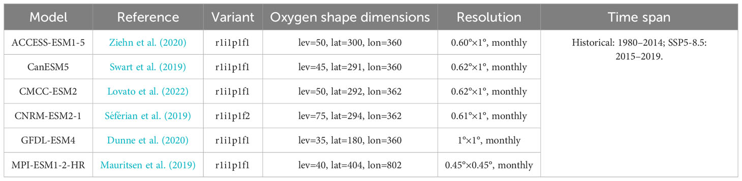
Table 1 List of CMIP6 models used in this study.

2.2 Data processing and matching

Considering the accuracy and reliability of measured DO data, it was important to perform data cleaning. WOD18 contained some erroneous data such as incorrect units and instrument failures, which needed to be removed. Therefore, we applied additional quality control rules as suggested by Schmidtko et al. (2017). These rules include the following: (1) removing profiles with a difference of less than 5 μmol kg⁻¹ between the maximum and minimum observed oxygen, (2) removing profiles with oxygen differences of less than 0.5 μmol kg⁻¹ within 18 depth levels, (3) removing profiles with less than 100 μmol kg⁻¹ oxygen at the surface, and (4) removing profiles with supersaturation at depths deeper than 200 m as well as supersaturation above 115%. We calculated DO saturated solubility using sea temperature and salinity, following the method proposed by Garcia et al. (1992). The DO profiles after data correction had millions of data records. However, the raw DO data records were unevenly distributed in space and time, thus directly modeling with these profile data could lead to spatiotemporal autocorrelation and overfitting due to excessive use of near-neighbor values. Therefore, we mapped the DO profile data into a 0.5°×0.5° grid at monthly average scales, and utilized a vertical interpolation method proposed by Reiniger and Ross (1968) to standardize the data into 50 depth levels (same as SODA v3.4.2 shape dimensions). Ultimately, we performed a point-to-point matching method to combine gridded in situ DO (DO_{in situ}), environmental variables from reanalysis data and DO from CMIP6 models (including DO_CMIP6-Mean and DO_CMIP6 from each sub-model) and generated multiple data samples with 285,729 records that could be used for model development and DO estimation comparison.

2.3 Spatiotemporal statistics of DO dataset

The spatial range of the Indian Ocean in this study covered 21°E–151°E and 50°S–27°N. To explore regional differences, the Indian Ocean was divided into four regions based on the WOD18 sea basin rules: the AS and BB in 10°N–27°N, the Equatorial Indian Ocean (EIO) in 10°N–10°S, and the Southern Indian Ocean (SIO) in 10°N–50°S.

The spatial distribution of DO_{in situ} established in section 2.2 is shown in Figure 1. Each grid had an average of 55 ± 52 observation points, and spatial mean DO concentration was 180.2 ± 59.9 μmol kg⁻¹. The AS, EIO, and SIO regions contained relatively dense DO records, with over 27,000, 71,000, and 184,000 observations, respectively, whereas the BB region had sparse DO records with only approximately 3,000 observations. By analyzing box plots (Figure 1D), it was observed that DO_{in situ} were not normally distributed. Therefore, we conducted a statistical analysis of DO_{in situ} distribution using the median and interquartile range (IQR). Median DO concentrations in the AS, BB, EIO, SIO, and total Indian Ocean were 49.4 μmol kg⁻¹ (IQR = 153.7 μmol kg⁻¹), 41.2 μmol kg⁻¹ (IQR = 129.1 μmol kg⁻¹), 121.0 μmol kg⁻¹ (IQR = 104.0 μmol kg⁻¹), 215.9 μmol kg⁻¹ (IQR = 51.5 μmol kg⁻¹), and 196.3 μmol kg⁻¹ (IQR = 92.3 μmol kg⁻¹), respectively.

FIGURE 1

Figure 1 Spatiotemporal statistics of measured DO (DO_{in situ}) in the Indian Ocean. Spatial distribution of (A) observation numbers and (B) mean DO_{in situ}. (C) Observation numbers and (D) boxplots of DO_{in situ} in the Arabian Sea (AS), the Bay of Bengal (BB), the Equatorial Indian Ocean (EIO), the Southern Indian Ocean (SIO), and total Indian Ocean. In (D), the orange line represents the median values of DO_{in situ}, and the green triangle represents the mean values of DO_{in situ}. (E) Annual observation numbers of DO_{in situ} and (F) vertical observation numbers of DO_{in situ}. (G) Annual median DO_{in situ} in 1980–2019 and (H) vertical median DO_{in situ} at depths of 0–5,395 m (50 depths). The light blue area enveloping the curve in (G) represents the annual interquartile ranges (IQR) of DO_{in situ}, and the light orange area enveloping the curve in (H) represents the vertical IQR of mean DO_{in situ}.

In terms of the temporal sampling, the number of DO records in 1995 exceeded 60,000 due to the large-scale scientific research program organized in that year, while the number of observations in other years was less than 10,000. In terms of the vertical sampling, the number of DO observations decreased with increasing depth. DO observations in the upper 1,000 m accounted for 80% of the total amount. DO concentration exhibited significant gradient change with two minimum values appearing at 100–300 m and 1,200–1,400 m, accompanied by a large IQR with 100–160 μmol kg⁻¹.

We further investigated the spatiotemporal correlations between DO_{in situ} and oceanic environmental factors (Table 2). DO had low-level spatiotemporal correlations with most variable factors, reflecting the extremely complicated non-linear relationship between DO and the marine environment in the Indian Ocean. However, DO had great correlations with temperature (r = –0.70, p < 0.01) and salinity (r = –0.85, p < 0.01) at depths of 1000-2000 m, and had a great negative correlation with temperature (r = −0.63, p <0.01) below 2000 m. These results show that, despite the fact that the distribution of measured oxygen is quite sparse in the mid-deep sea, it is possible to reconstruct the complete vertical DO structure using temperature and salinity. In addition, although the correlations between DO and the variables reflecting ocean circulation (u, v, and w) and sea–air interaction (ssh, taux, and tauy) were weak, the relevance between DO and these factors is relatively modest; thus, these composite variables also contribute to establish a more stable oxygen field.

TABLE 2

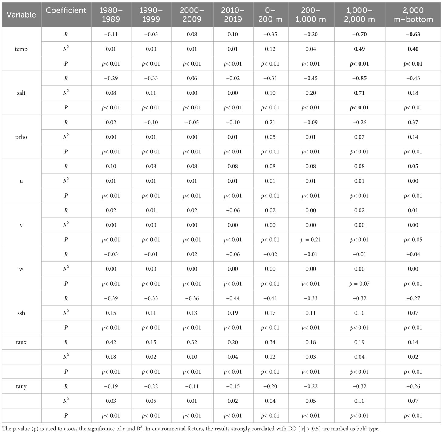
Table 2 Correlation coefficients (r) and coefficients of determination (R²) between DO_{in situ} and ocean environmental factors.

In summary, the correlations between DO and environmental variables were not very high. In the following text, we consider choosing high-performance machine learning techniques to fit multiple marine variables with DO_{in situ}, in an attempt to use machine learning algorithms to demonstrate their strong ability to complete the DO modeling task.

3 Methods

3.1 Machine learning algorithms

To thoroughly compare the performance of machine learning models, we selected ordinary least squares linear regression (OLR), multiple-layer perceptron (MLP) (LeCun et al., 2015), AdaBoost (ADB) (Freund and Schapire, 1997), gradient boosting (GB) (Friedman, 2001), RF (Breiman, 2001), and extremely randomized trees (ERT) (Geurts et al., 2006) for DO modeling in this study.

We utilized OLR as the baseline model. OLR is a simple but classical multivariate regression algorithm. It finds the best-fitting linear relationship between the input features and the target variable. MLP is a standard type of artificial neural network characterized by its composition of multiple layers of interconnected nodes, enabling it to effectively model intricate non-linear relationships. The training process of an MLP involves techniques like activation function, backpropagation, and gradient descent, which are essential for adjusting the network’s weights to minimize prediction errors.

ADB and GB are two well-known “Boosting” algorithms that involve sequential construction of decision trees. “Boosting” is an ensemble learning technique that combines multiple weak regressors to create a strong and high-accuracy regression model. It works by sequentially training regressors and giving more emphasis to data points with larger prediction errors, and the final regression prediction is typically a weighted combination of individual regressor predictions. The key distinction in those two algorithms is in the way they adapt to errors and construct their ensemble. ADB iteratively focuses on challenging data points, while GB constructs a sequence of trees with each one reducing the residual errors of the previous models. This leads to nuanced differences in their predictive performance.

RF and ERT are two well-known algorithms that employ parallel construction of decision trees, and they give the results by averaging the predictions of multiple trees. RF builds an ensemble of decision trees by bootstrap aggregating (named as “Bagging”) the data and uses an optimal splitting strategy for each node using a random subset of features. The “Bagging” technique creates multiple subsets (bootstrap samples) of the training data by randomly selecting data points with replacement. It aims to reduce overfitting and variance and enhance model stability. ERT is similar to RF but with a higher degree of randomness. It randomly uses selecting features for node splitting and constructs subtrees using entire samples, making it computationally efficient while maintaining good predictive performance.

3.2 Model development and DO construction

In the model development, we randomly divided the matched-up DO dataset mentioned in section 2.2 into training and validation subsets in the ratio of 8:2, and established multiple machine learning models using spatiotemporal information, environmental factors, and DO_{in situ} from the training set, which can be represented as follows:

$\begin{array}{ll}{X}_{ST}=[year, month,depth,longitude,latitude,bathymetry]& (1)\end{array}$

$\begin{array}{ll}{X}_{env}=[temp,salt,prho,u,v,w,ssh,taux,tauy]& (2)\end{array}$

$\begin{array}{ll}\widehat{DO}=f(X_{ST},X_{env};D{O}_{in situ})& (3)\end{array}$

where $f(·)$ represents the machine learning model, $X_{ST}$ represents spatiotemporal information, $X_{env}$ represents environmental factors in reanalysis data, and $D{O}_{in situ}$ represents the actual DO values fitted by the model.

This study utilizes the coefficient of determination (R²), root-mean-square error (RMSE), mean absolute error (MAE), and mean bias (MB) as accuracy evaluation metrics when comparing DO_Modeled and DO_CMIP6 with DO_{in situ}. R² reflects the closeness of the linear relationship of the model values and the field measurement data, RMSE reflects the deviation of the model values from the field measurement data, MAE reflects the absolute differences between the model values, and the field DO_{in situ} approximates the target true values. The evaluation indices are calculated as follows:

$\begin{array}{ll}{R}^2=1-\frac{{\sum }_{i=1}^N{(y_i-{\widehat{y}}_i)}^2}{{\sum }_{i=1}^N{(y_i-\overline{y})}^2}& (4)\end{array}$

$\begin{array}{ll}RMSE=\sqrt{\frac{{\sum }_{i=1}^N{(y_i-{\widehat{y}}_i)}^2}{N}}& (5)\end{array}$

$\begin{array}{ll}MAE=\frac{{\sum }_{i=1}^N\left|y_i-{\widehat{y}}_i\right|}{N}& (6)\end{array}$

$\begin{array}{ll}MB=\frac{{\sum }_{i=1}^N(y_i-{\widehat{y}}_i)}{N}& (7)\end{array}$

where $y_i$ represents the true value, ${\widehat{y}}_i$ represents the predicted value, $\overline{y}$ represents the mean true value, and $N$ represents the number of samples.

We utilized the scikit-learn package in Python 3.8.13 to perform DO modeling using six algorithms. The model performance metrics and hyper-parameter information are shown in Table 3. The results show that the ERT model has the highest performance, and the parallel ensemble trees methods (RF and ERT) perform better than the sequential ensemble trees methods (ADB and GB).

TABLE 3

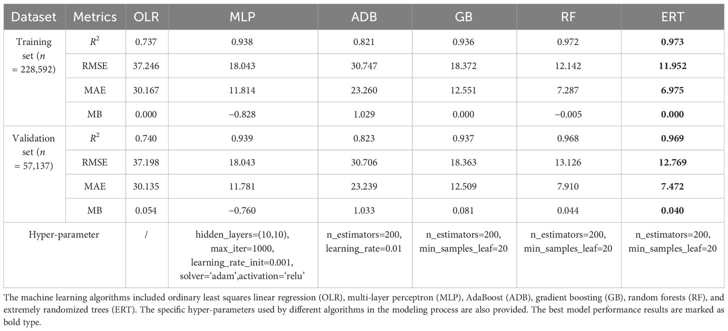
Table 3 The performances of machine learning models evaluated with the training set and validation set.

We further used feature importance (FI) to compare the predictive differences between the RF and ERT models. The FI of the ensemble trees serves as an indicator of the importance of modeling factors. Here, we display the FI for both the ERT and RF models (Table 4). In the FI results of the ERT model, we selected the top 1/3 of the total 15 prediction factors as the most important factors. By removing spatial variables (latitude and depth), the remaining three variables—temperature, salinity, and seawater density—were the most important marine environmental factors that have a significant impact on DO. In addition, the FI ranking of the RF model was different, but similar opinions were expressed. Therefore, we confidently accepted the FI results and focused subsequent driven factor analysis mainly on temperature, salinity, and seawater density.

TABLE 4

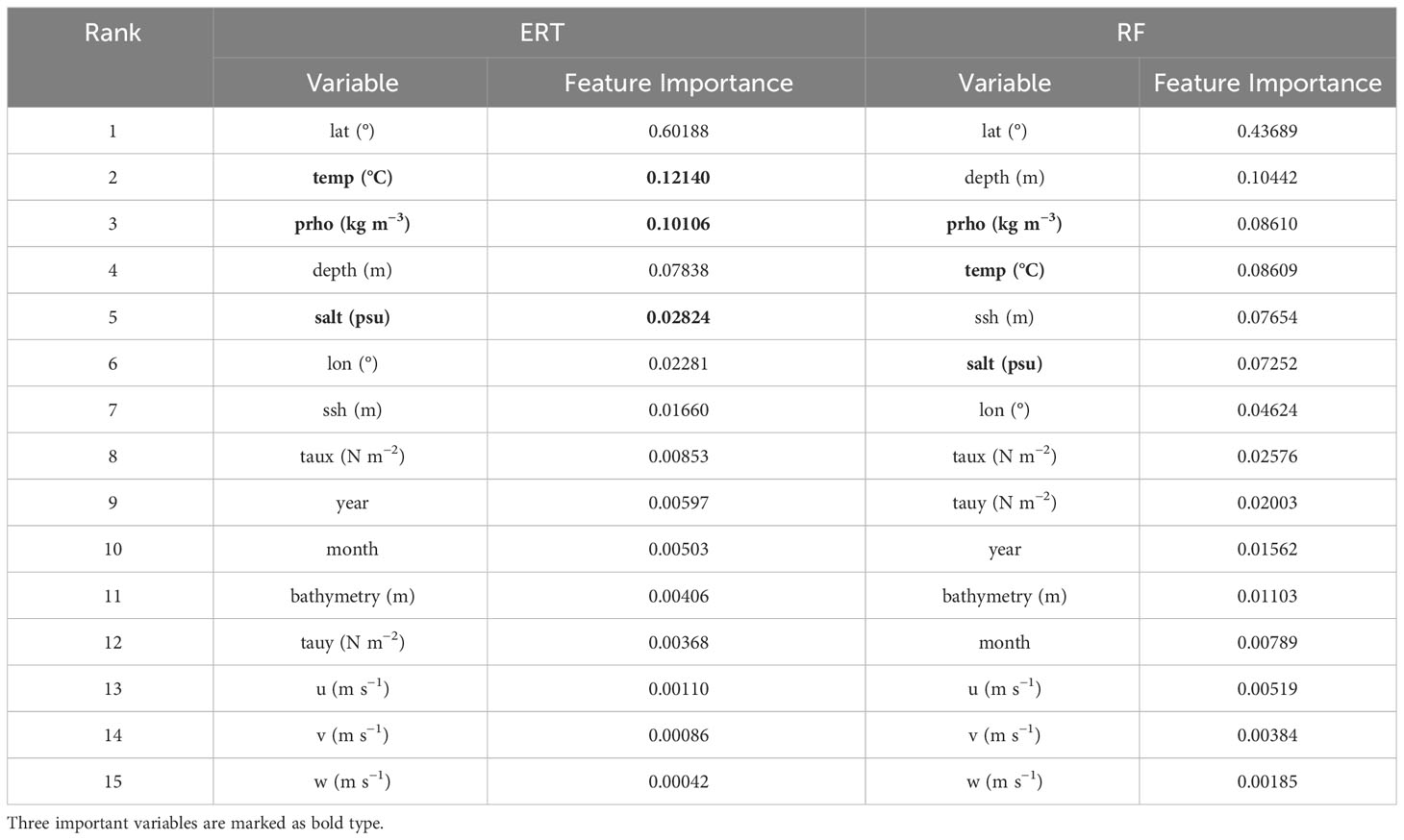
Table 4 The feature importance of DO models developed by extremely randomized trees (ERT) and random forests (RF) algorithms.

We conducted data reconstruction experiments using both the RF and ERT models (distinguished by DO_RF and DO_ERT). As shown in the results in Figure S1, we found that DO_RF spatial distribution has some local anomalies (characterized by longitudinal stripes), and DO_RF significantly underestimates the extent of the OMZs in the AS and BB. However, DO_ERT is less affected by local disturbances and exhibits similar OMZs distributions as the previous study (Zhou et al., 2022).

Therefore, we utilized the developed ERT model as the best model to input the entire dataset of DO samples, generating prediction results labeled as DO_Modeled. Furthermore, we inputted complete reanalysis data along with spatiotemporal information into the ERT model, obtaining a reconstructed DO dataset (DO_4D-Modeled) with the following shape dimensions: time=480, lev=50, lat=154, and lon=260. DO_4D-Modeled serves as the foundation for discussing the spatiotemporal distribution and variations of oxygen in the Indian Ocean in 1980–2019.

3.3 Calculation of DO content, trend, and change rate

Based on DO_4D-Modeled, we further estimated DO content, trend, and change rate to reveal the entire DO variations in the Indian Ocean. To assist with these calculations, we created grid area files and water column height files and calculated ocean volume, DO content, and trend using CDO. The method used for these calculations will be described in detail below.

To obtain spatial distribution of DO content ($I_{DO}^S$) and total DO content ($I_{DO}$), we use single integrals and double integrals of total water-column volume for DO grid at time $t$, respectively. These calculation formulas are as follows:

$\begin{array}{ll}{I}_{DO}^S(\text{t})={\int }^{}DO(t)\rho (t)dH& (8)\end{array}$

$\begin{array}{ll}{I}_{DO}(\text{t})={\iint }^{}DO(t)\rho (t)dAdH& (9)\end{array}$

where $DO(t)$ represents the DO concentration of the cell grid at the depth of each layer at time $t$, and $\rho (t)$ represents the seawater potential density of the cell grid at the depth of each layer at time $t$. $dH$ represents the water column height corresponding to the depth of each layer. $dA$ represents the cell area corresponding to DO grid at sea level. We assume that the grid area at different depths remains unchanged, and the grid area at each depth is consistent with surface grid area; thus, grid area error caused by depth is ignored.

To obtain the spatial trend of DO content ($T_{DO}^S$) and trend of total DO content ($T_{DO}$), we use the linear regression method to estimate the linear trend of $I_{DO}^S$ and $I_{DO}$.

$\begin{array}{ll}{T}_{DO}^S=\frac{{\sum }_{t=1}^n(t-\overline{t})(I_{DO}^S(t)-\overline{I_{DO}^S})}{{\sum }_{t=1}^n{(t-\overline{t})}^2}& (10)\end{array}$

$\begin{array}{ll}{T}_{DO}=\frac{{\sum }_{t=1}^n(t-\overline{t})(I_{DO}(t)-\overline{I_{DO}})}{{\sum }_{t=1}^n{(t-\overline{t})}^2}& (11)\end{array}$

where $\overline{t}= \frac{1}{n}{\sum }_{i=1}^{n}t$, $\overline{I_{DO}^S}= \frac{1}{n}{\sum }_{i=1}^n{I}_{DO}^S(t)$, and $\overline{I_{DO}}= \frac{1}{n}{\sum }_{i=1}^n{I}_{DO}(t)$.

We perform a significance test on DO content trend using the method introduced by Santer et al. (2000). Firstly, we calculate the standard deviation of the linear regression residuals $e(t)$, denoted as $S_e$, along with the standard deviation of the regression coefficient $a_1$, denoted as $S_a$. These calculation formulas are as follows:

$\begin{array}{ll}{\widehat{I}}_{DO}(t)=a_{1}t+a_0& (12)\end{array}$

$\begin{array}{ll}e(t)=I_{DO}(t)-{\widehat{I}}_{DO}(t)=I_{DO}(t)-(a_{1}t+a_0)& (13)\end{array}$

$\begin{array}{ll}{S}_e=\sqrt{\frac{{\sum }_{t=1}^{n}e{(t)}^2}{n-2}}& (14)\end{array}$

$\begin{array}{ll}{S}_a=\sqrt{\frac{S_e^2}{{\sum }_{t=1}^n{(t-\overline{t})}^2}}& (15)\end{array}$

Secondly, we obtain the statistical value $T_a$, calculated as $T_a=\frac{a_1}{S_a}$. $T_a$ follows a Student’s t-distribution with $n-2$ degrees of freedom ($n$ represents total time counts). To determine the significance of the slope $a_1$, we conduct a t-test on the statistical value $T_a$ (Santer et al., 2000). This process takes into account the probability on both sides of the distribution and calculates a two-tailed p-value for $T_a$. We set the significance level to 0.05, and if the p-value is less than 0.05, we can conclude that DO content trend is statistically significant at the 95% confidence level; otherwise, it is not significant.

Finally, the uncertainty of DO content trend (${\sigma }_{DO}$) is defined as twice the standard deviation of the regression coefficient $S_a$:

$\begin{array}{ll}{\sigma }_{DO}=2·S_a=2\sqrt{\frac{S_e^2}{{\sum }_{t=1}^n{(t-\overline{t})}^2}}& (16)\end{array}$

To obtain the change rate of the DO content in grid cell ($R_{DO}$), we use the ratio of DO trend to ocean volume to estimate $R_{DO}$, and its calculation formula is as follows:

$\begin{array}{ll}{R}_{DO}=\frac{T_{DO}\pm {\sigma }_{DO}}{V}& (17)\end{array}$

where ocean volume $V={\int }^{ }dV= \iint dAdH$.

4 Results

4.1 Model assessment and data evaluation

4.1.1 Model performance assessment

To analyze the disparity between DO_Modeled and DO_CMIP6-Mean relative to DO_{in situ}, we examined their spatial distribution of RMSE and MB, and compared the data using scatter plots. The overall model performance results are shown in Figure 2. DO_Modeled on the training set closely approximated DO_{in situ}, with an R² of 0.973, an RMSE of 12.0 μmol kg⁻¹, and an MAE of 7.0 μmol kg⁻¹. DO_Modeled on the validation set also simulated DO_{in situ} well, with an R² of 0.969, an RMSE of 12.8 μmol kg⁻¹, and an MAE of 7.5 μmol kg⁻¹. In contrast, DO_CMIP6-Mean was relatively not close to DO_{in situ}, with an R² of 0.838, an RMSE of 29.3 μmol kg⁻¹, and an MAE of 18.9 μmol kg⁻¹.

FIGURE 2

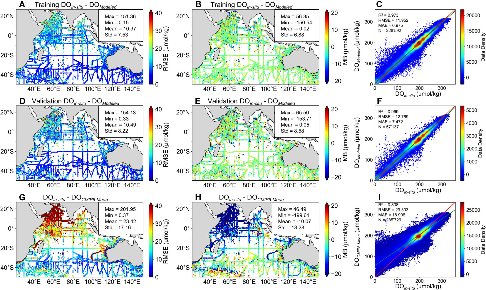
Figure 2 Spatial precision results of DO data established by the machine learning model (DO_Modeled) and mean CMIP6 DO data (DO_CMIP6-Mean) and their comparison results with measured DO data (DO_{in situ}). The precision evaluations of (A–C) DO_Modeled on the training set, (D–F) DO_Modeled on the validation set, and (G–I) DO_CMIP6-Mean include the spatial distribution of root-mean-square error (RMSE) and mean bias (MB), and scatter plots for comparison with DO_{in situ}. In the scatter plots, red lines represent the 1:1 line and green lines represent the actual fitting lines.

In terms of spatial precision: the mean RMSE results of DO_Modeled on the training set, DO_Modeled on the validation set, and DO_CMIP6-Mean were 10.4 μmol kg⁻¹, 10.5 μmol kg⁻¹, and 23.4 μmol kg⁻¹, respectively. The mean MB results of DO_Modeled on the training set, DO_Modeled on the validation set, and DO_CMIP6-Mean were 0.02 μmol kg⁻¹, 0.05 μmol kg⁻¹, and −10.07 μmol kg⁻¹, respectively. From the spatial results of RMSE, it can be seen that simulating DO in the AS and the BB is quite difficult due to their complex ocean dynamics (McCreary et al., 2013). From the spatial results of MB, the prediction residuals of DO_Modeled were relatively uniform, indicating that the ERT model performance is quite stable. However, the mean CMIP6 model did not perform well in simulating spatial DO distribution. There were many differences between ensemble CMIP6 model predictions and observations, such as most models overestimating DO in the AS and BB, and the CNRM-ESM2-1 and MPI-ESM1-2-HR model underestimating DO in several areas (Figure S2).

To further compare the spatiotemporal precisions of DO_Modeled and DO_CMIP6-Mean, we analyzed RMSE and MB of DO_Modeled and DO_CMIP6-Mean in subregions by decades and depths (Figure 3). Our ERT model predictions exhibited great simulation performance on the training set and validation set, outperforming the mean CMIP6 model. Despite the unbalanced spatiotemporal DO_{in situ} distribution, the DO_Modeled simulation quality remained unaffected by variations in sample weighting across space and time, demonstrating the robustness of the ERT-based DO model.

FIGURE 3

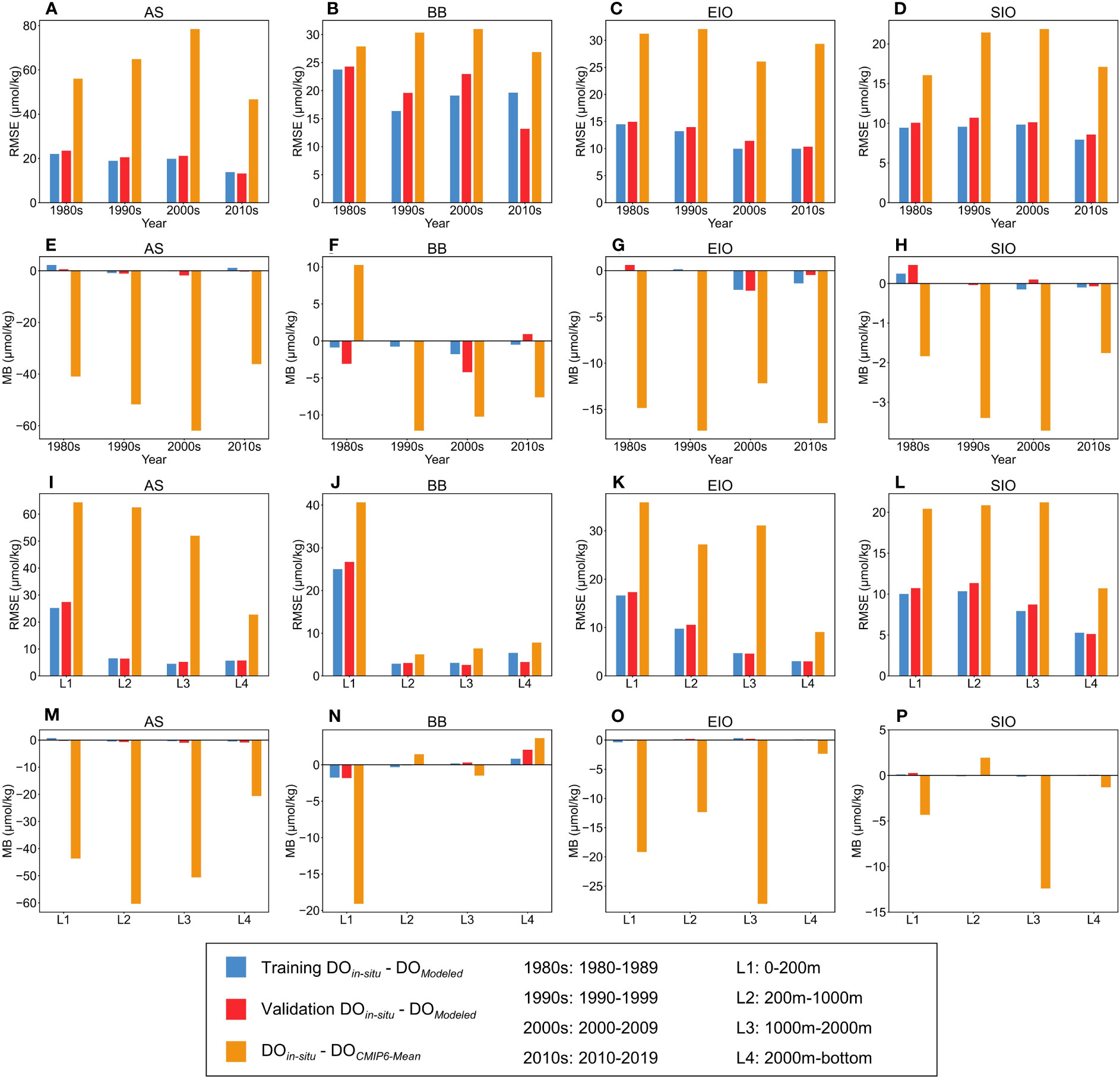
Figure 3 Root-mean-square errors (RMSEs) and mean bias (MB) of DO data established by the machine learning model (DO_Modeled) on the training set, DO_Modeled on the validation set, and mean CMIP6 DO data (DO_CMIP6-Mean) in the Arabian Sea (AS), Bay of Bengal (BB), Equatorial Indian Ocean (EIO), and Southern Indian Ocean (SIO) regions by different years and depth layers. (A–D) RMSE and (E–H) MB comparison in different years. (I–L) RMSE and (M–P) MB comparison in different depth layers. Blue, red, and orange bars represent the RMSE of the DO_Modeled in the training set, DO_Modeled in the validation set, and DO_CMIP6-Mean, respectively. 1980s, 1990s, 2000s, and 2010s represent 1980–1989, 1990–1999, 2000–2009, and 2010–2019, respectively. L1, L2, L3, and L4 represent 0–200 m, 200–1,000 m, 1,000–2,000 m, and 2,000 m–bottom, respectively.

4.1.2 Accuracy evaluation of derived DO data

The results in section 4.1.1 provide an assessment of the data-driven model and CMIP6 models, but these statistical metrics have limitations in quantifying decadal oxygen change across various regions and depth layers. To investigate the spatiotemporal variations of the simulations, we used the validation set to perform independent evaluations in the ERT model and CMIP6 models.

Here, we display the time series of annual mean DO (including DO_{in situ}, DO_Modeled, and DO_CMIP6) for different regions and depth layers (Figure 4). It should be noted that this section considers the independent evaluation on the validation set, and the DO value at each measured point results from unevenly sparse sampling. From a geostatistical perspective, the sampling records contain unbalanced observations. Although DO_{in situ} on the validation set exhibited decadal variations, they cannot directly represent the mean spatiotemporal DO variations in each region.

FIGURE 4

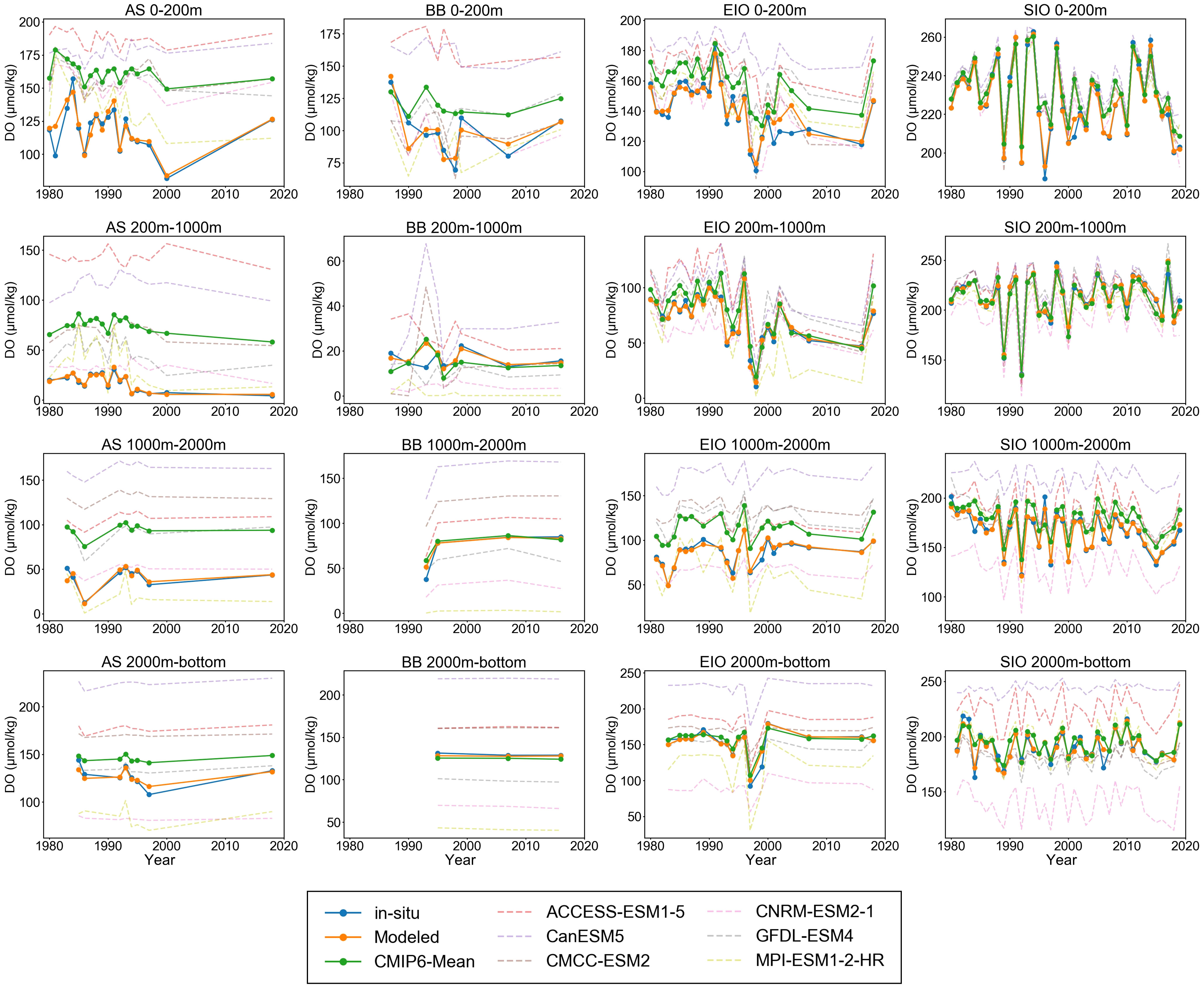
Figure 4 Annual mean variations of measured DO (DO_{in situ}), DO predicted by the machine learning model (DO_Modeled), and CMIP6 DO (including mean values, ACCESS-ESM1-5, CanESM5, CMCC-ESM2, CNRM-ESM2-1, GFDL-ESM4, and MPI-ESM1-2-HR) on the validation set in the Arabian Sea (AS), Bay of Bengal (BB), Equatorial Indian Ocean (EIO), and Southern Indian Ocean (SIO) regions at depths of 0–200 m, 200–1,000 m, 1,000–2,000 m, and 2,000 m–bottom.

The DO predictions from different CMIP6 models were not consistent with DO_{in situ}. CMIP6 models exhibited systematic overestimation or underestimation of oxygen variations, and their mismatches were evident in several regions, limiting the effectiveness of DO_CMIP6-Mean simulations, as well as resulting in different trend variations compared to DO_{in situ}. In contrast, DO_Modeled closely approximated DO_{in situ} in time series. Despite not being trained on the validation set, our model successfully predicted trends that align with DO observations. This suggests that the ERT model can proficiently capture spatiotemporal DO variations. Consequently, we applied this model to reconstruct the DO_4D-Modeled dataset, facilitating further discussions and analyses of the spatiotemporal DO patterns in the Indian Ocean.

4.2 Distributions and variations of DO

4.2.1 Spatiotemporal distributions of DO

Here, we analyzed spatial mean DO distributions at different depths (Figure 5) and mean DO time–depth profiles in each subregion (Figure 6). According to these results, spatial and vertical DO distributions in the Indian Ocean exhibit strong heterogeneity.

FIGURE 5

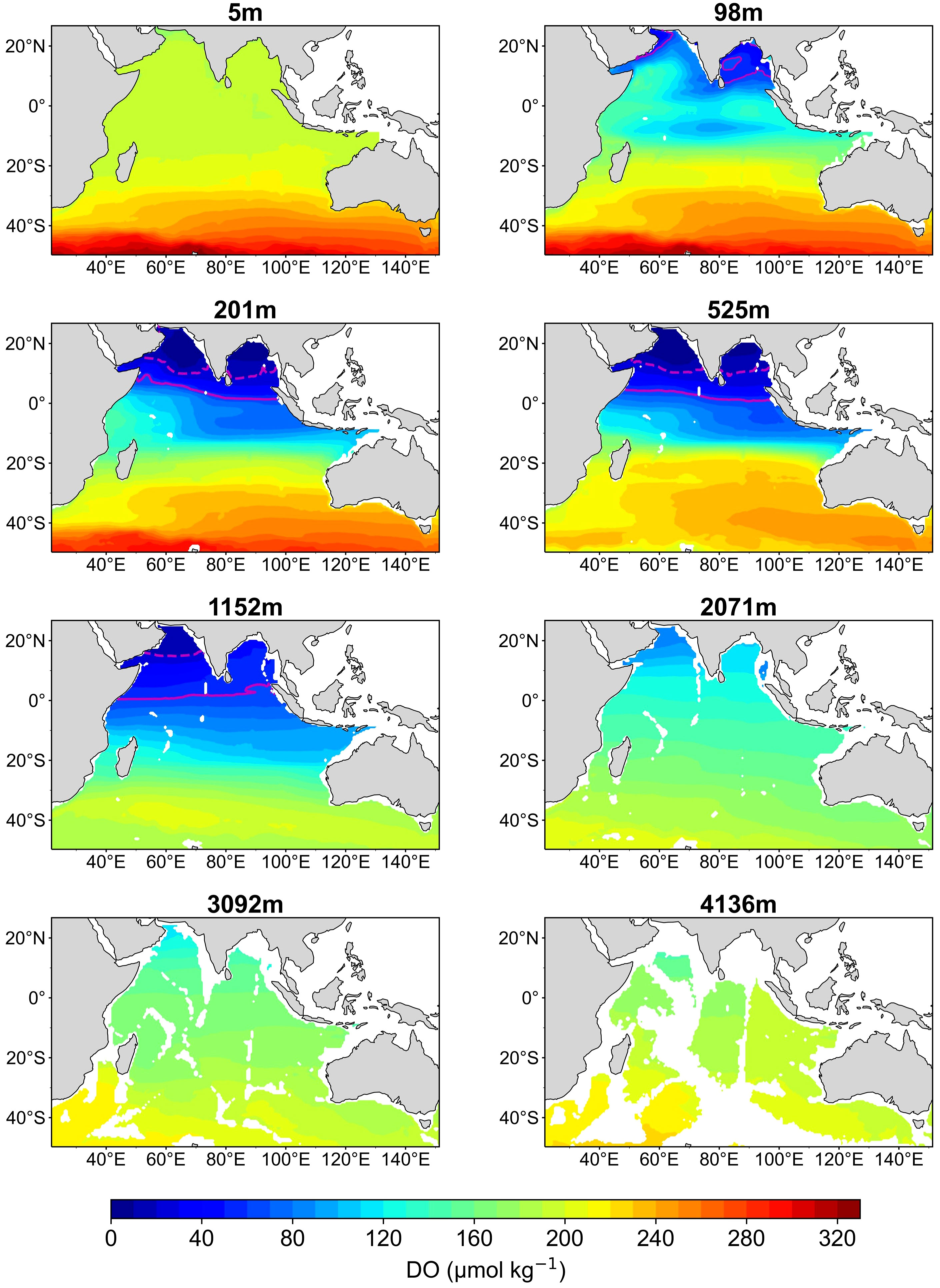
Figure 5 Spatial distribution of mean dissolved oxygen (DO) concentration at different depths in the Indian Ocean during 1980–2019. The solid line envelope and dotted line envelope in magenta represent the oxygen-minimum zones of DO ≤ 60 μmol kg⁻¹ and DO ≤ 20 μmol kg⁻¹, respectively.

FIGURE 6

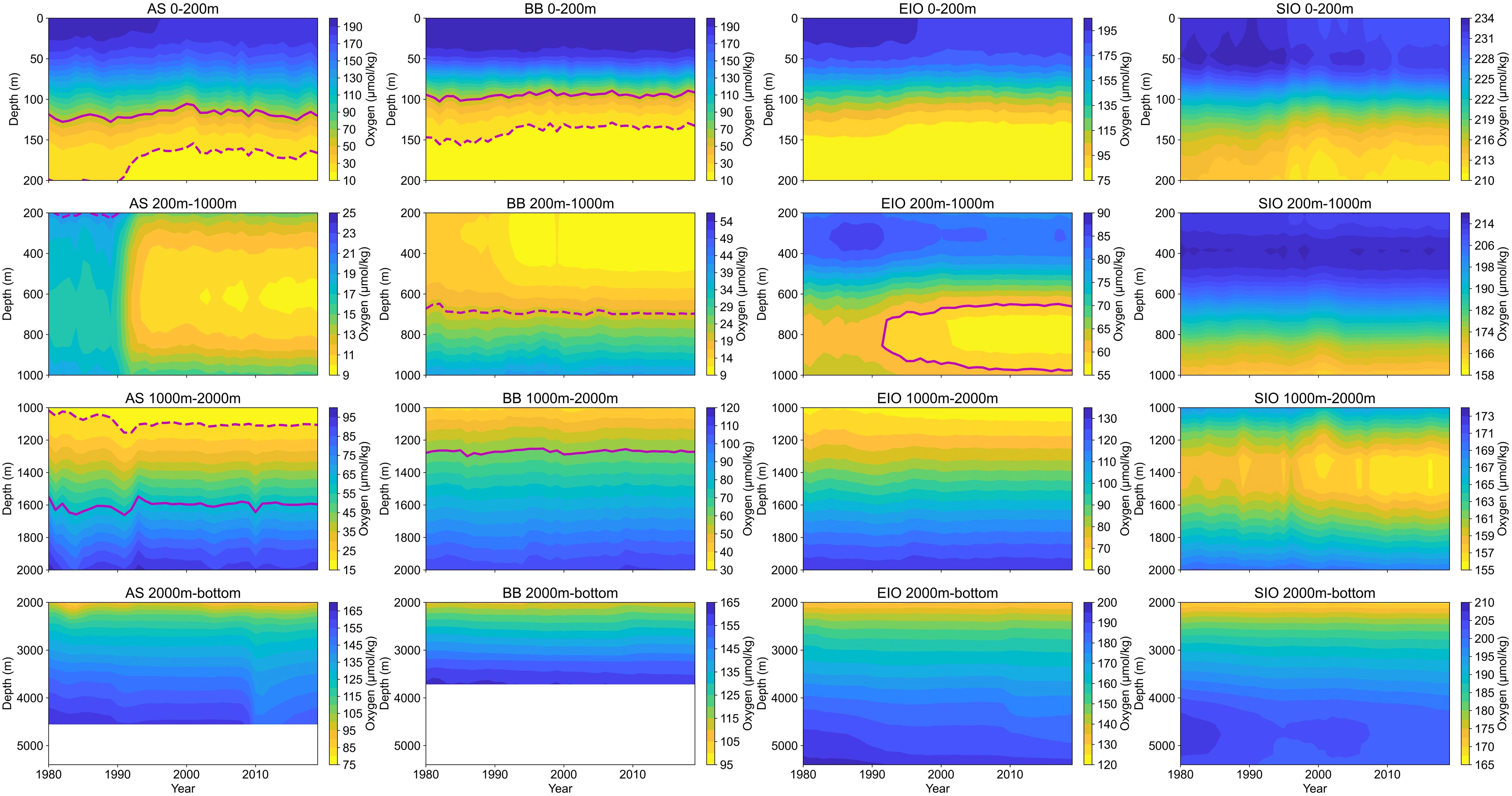
Figure 6 Time–depth profiles of annual mean dissolved oxygen (DO) in the Arabian Sea (AS), Bay of Bengal (BB), Equatorial Indian Ocean (EIO), and Southern Indian Ocean (SIO) during 1980–2019. For each depth, mean DO is obtained from the grid weighted average of DO concentrations in each subregion. The solid line enveloped and dotted line enveloped areas represent the oxygen-minimum zones of DO ≤ 60 μmol kg⁻¹ and DO ≤ 20 μmol kg⁻¹, respectively.

At 0–200 m, the DO ranges in the AS, BB, EIO, and SIO are 14–196 μmol kg⁻¹, 10–198 μmol kg⁻¹, 77–198 μmol kg⁻¹, and 210–233 μmol kg⁻¹, respectively. Although sea surface DO is in the state of supersaturation due to the rapid air–sea gas exchange, DO levels in the AS, BB, and EIO are lower than SIO. This discrepancy may be attributed to the oxygen loss caused by anthropogenic emissions and land-based nutrient inputs (Rixen et al., 2020; Naqvi, 2021).

DO gradually decreases at depths of 200–2,000 m, and extremely low DO regions are found in the AS and BB with the DO range of 9–102 μmol kg⁻¹ and 9–115 μmol kg⁻¹, respectively. Insufficient DO regions are also found in the EIO and SIO with the DO range of 56–133 μmol kg⁻¹ and 155–216 μmol kg⁻¹, respectively. The DO loss in the ocean interior may be attributed to weakened ventilation caused by stratification, leading to the large amount of oxygen consumption by remineralization and biological processes, and sufficient oxygen supply cannot be maintained due to the weakening of ocean subduction and vertical mixing (Portela et al., 2020; Buchanan and Tagliabue, 2021).

In the mid-deep sea below 2,000 m, DO levels exhibit an increase with depth. In these regions, DO ranges in the AS, BB, EIO, and SIO are 76–165 μmol kg⁻¹, 99–164 μmol kg⁻¹, 121–197 μmol kg⁻¹, and 165–205 μmol kg⁻¹, respectively. The DO rising in the mid-deep sea is caused by oxygen consumption weakening and oxygen supply by circulation (Levin, 2018; Oschlies et al., 2018).

4.2.2 Oxygen-minimum zones expansions

According to the time–depth profile of DO in the Indian Ocean (Figure 6), low-oxygen zones with DO less than 70 μmol kg⁻¹ are located in the AS, BB, and EIO at depths of 100–2,000 m. A previous study has indicated that ocean zones with DO levels below 60 μmol kg⁻¹ (OMZ60) will cause damage to marine biodiversity, and ocean zones with DO levels below 20 μmol kg⁻¹ (OMZ20) will be fatal to marine organisms (Vaquer-Sunyer and Duarte, 2008). Therefore, it is crucial to monitor the changes in both OMZ20 and OMZ60 to assess the state of marine hypoxia conditions.

To compare the vertical variation of two OMZs, we outlined the upper and lower boundaries of OMZ20 and OMZ60 in the time–depth profile. Vertical variation results demonstrate that OMZ20 and OMZ60 in the AS are located at depths of 150–1,100 m and 110–1,700 m, respectively, while those in the BB are located at depths of 130–700 m and 100–1,300 m, respectively. The OMZs in the AS exhibit greater thickness than those in the BB, with their upper and lower boundaries found at deeper depths than those of the BB. These findings suggest that hypoxia is more severe in the AS, possibly due to the combination effects of weaker downwelling, stronger biological consumption, and remineralization (Lachkar et al., 2019; Sarma et al., 2020).

In terms of temporal variation, OMZs in the AS and BB slowly expanded towards shallow waters, with their upper boundaries constantly moving towards the upper ocean. After the 1990s, the expansion of OMZ20 in the AS and BB became more rapid, with the upper boundary in the AS and BB expanding from 210 m to 160 m and 150 m to 130 m, respectively. During the same period, OMZ60 in the EIO began to expand significantly at 700–1,000 m, indicating that the low-oxygen waters had expanded from the AS and BB to the EIO. However, the expansion of OMZs in the AS, BB, and EIO has started to decelerate since the 2000s, and OMZs have formed relatively stable upper and lower boundaries in the vertical direction.

4.2.3 Spatiotemporal variations of DO

We calculated the spatial and vertical DO concentration trends based on DO spatiotemporal distribution (Figures 7, S3) and further analyzed the spatiotemporal DO variations in different parts of the Indian Ocean during the past 40 years.

FIGURE 7

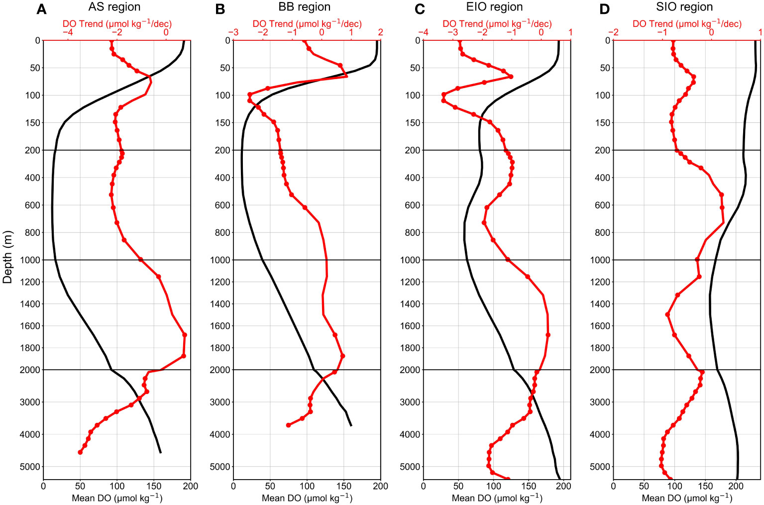
Figure 7 Vertical dissolved oxygen (DO) trend (red lines) and mean DO (black lines) in the (A) Arabian Sea (AS), (B) Bay of Bengal (BB), (C) Equatorial Indian Ocean (EIO), and (D) Southern Indian Ocean (SIO). The red scatter points represent that DO trends within these depth layers are statistically significant at a 95% confidence level (p < 0.05).

At 0–200 m, DO levels in all regions exhibit large downward trends. The maximum DO decline trends in the mixed layer of the AS, BB, and EIO are −2.2 μmol kg⁻¹ dec⁻¹, −2.5 μmol kg⁻¹ dec⁻¹, and −3.3 μmol kg⁻¹ dec⁻¹, respectively. The vertical DO decrease is relatively small in the SIO, with the maximum DO decline trend up to −0.8 μmol kg⁻¹ dec⁻¹. The DO decline trend slows at depths of 50–100 m, possibly due to vertical mixing transporting surface DO-rich water to this depth range, offsetting some of the DO loss. However, there is a special case where DO increases in the BB at depths of 40–80 m, up to 0.9 μmol kg⁻¹ dec⁻¹.

Owing to the complex effect at 200–1,000 m, seawaters have different DO changes. It was observed that DO levels not only decrease at these depths but also increase in the BB and SIO. In the AS, DO remains in a consistently high decreasing state, with the trend ranging from −2.2 to −1.0 μmol kg⁻¹ dec⁻¹. DO decline trends in the BB and EIO began to moderate, with the trend up to −1.4 μmol kg⁻¹ dec⁻¹ and −1.9 μmol kg⁻¹ dec⁻¹, respectively. DO levels increased in the BB at 800–1,000 m and the SIO at 400–800 m, with the trend up to 0.2 μmol kg⁻¹ dec⁻¹.

At 1,000–2,000 m, DO trend variations are exactly opposite to those at the upper 200–1,000 m, which may be attributed to stronger stratification below 1,000 m, leading to DO differences in the upper and deeper ocean. DO increases in the northern and equatorial parts of the Indian Ocean, with the trend up to 0.8 μmol kg⁻¹ dec⁻¹ in the AS, 0.7 μmol kg⁻¹ dec⁻¹ in the BB, and 0.2 μmol kg⁻¹ dec⁻¹ in the EIO, but decreases in the SIO with the trend of −0.9 μmol kg⁻¹ dec⁻¹ to −0.3 μmol kg⁻¹ dec⁻¹.

At 2,000 m–bottom, DO decline in the AS is unusually strengthened with the trend up to −3.5 μmol kg⁻¹ dec⁻¹, which has reached the maximum oxygen loss trend in the whole water column. The DO in the BB changes from an increasing to a decreasing trend, and the DO decreasing trend in the EIO and SIO is also enhanced gradually. Overall, DO decline in the BB, EIO, and SIO is relatively low compared to the subsurface ocean, with the trend up to −1 μmol kg⁻¹ dec⁻¹ in the BB and SIO and −1.8 μmol kg⁻¹ dec⁻¹ in the EIO.

Through analysis results of the DO trend at full depth of the Indian Ocean, DO decreasing regions appear in subsurface and high-depth waters with the DO decline trend up to −1.5 μmol kg⁻¹ dec⁻¹, and DO increasing regions appear in thermocline and mid-depth waters. DO change trends are exactly the opposite between the upper and the deeper ocean at the boundary of 1,000 m, which may be due to the strong stratification under the thermocline (Li et al., 2020; Sallée et al., 2021). In addition, we found that the areas with relatively high DO loss mainly existing in the AS at 0–1,000 m and 2,000 m–bottom, BB at 0–200 m, and EIO at 0–1,000 m and 2,000 m–bottom, and the areas with DO increasing mainly existing in the AS at 1,000–2,000 m, BB at 40–80 m and 800–2500 m, EIO at 1,000–2,000 m, and SIO at 400–800 m. By comparing the DO trends in different areas, the maximum DO decrease trend ranking is AS > EIO > BB > SIO, and the maximum DO increase trend ranking is BB > AS > EIO = SIO.

5 Discussion

5.1 Driver analysis of DO variations

5.1.1 Drivers of DO decrease

Previous studies have indicated that DO variations are caused by changes in two components: oxygen solubility and AOU, and deoxygenation is dominated by AOU (Schmidtko et al., 2017; Oschlies et al., 2018). However, AOU involves multiple interactions that are challenging to assess, and solubility-induced oxygen loss is more readily evaluated. This section mainly analyzes the AS and EIO regions with the most severe DO declines, and predominantly addresses parameters related to DO solubility, including temperature and salinity governing solubility, and density closely associated with stratification effects (Figures 8, 9, S4, S6).

FIGURE 8

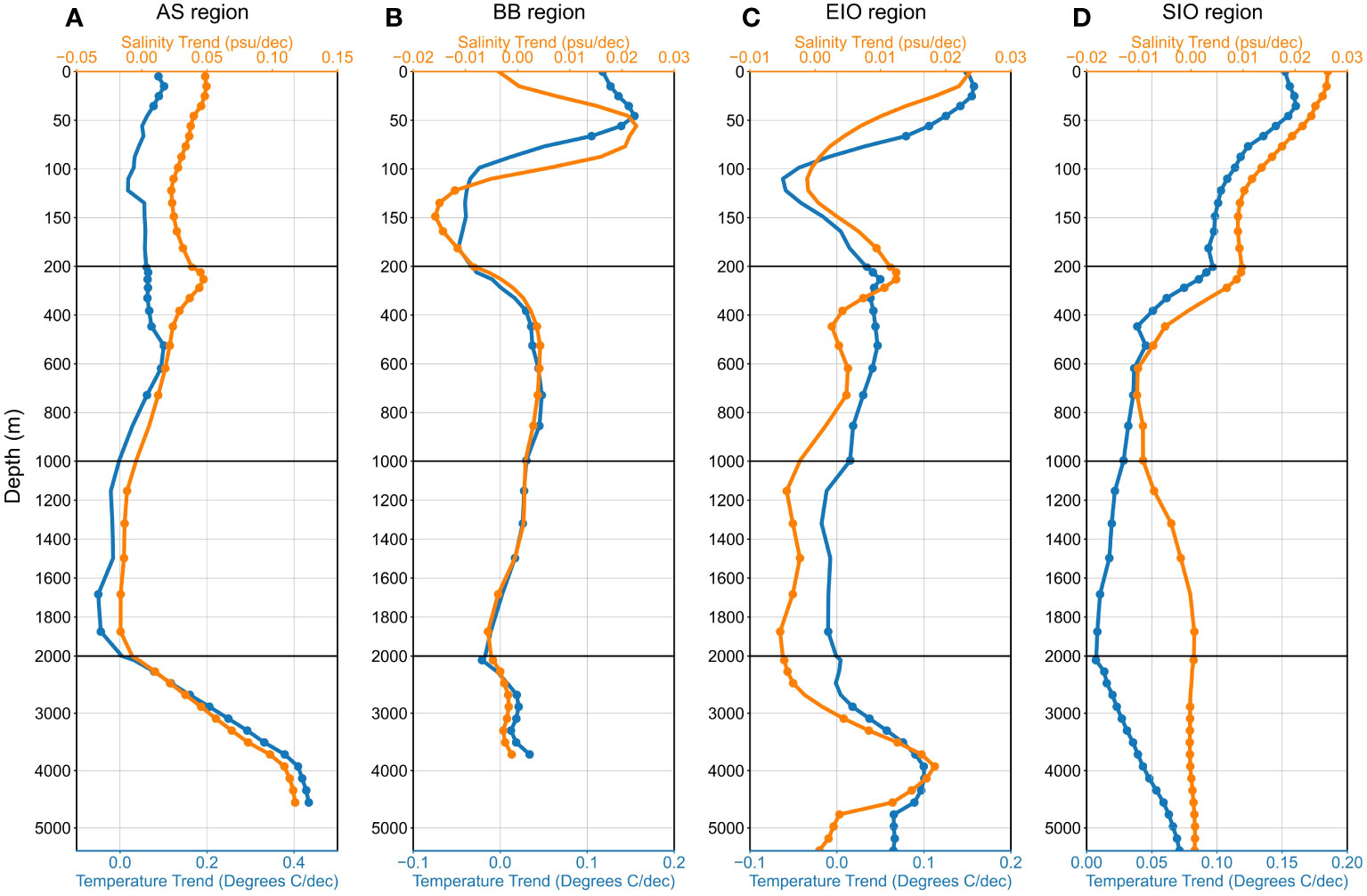
Figure 8 Vertical temperature trend (blue lines) and salinity trend (orange lines) in the (A) Arabian Sea (AS), (B) Bay of Bengal (BB), (C) Equatorial Indian Ocean (EIO), and (D) Southern Indian Ocean (SIO). The blue scatter points and the orange scatter points represent that temperature trends and salinity trends within these depths are statistically significant at a 95% confidence level (p < 0.05), respectively.

FIGURE 9

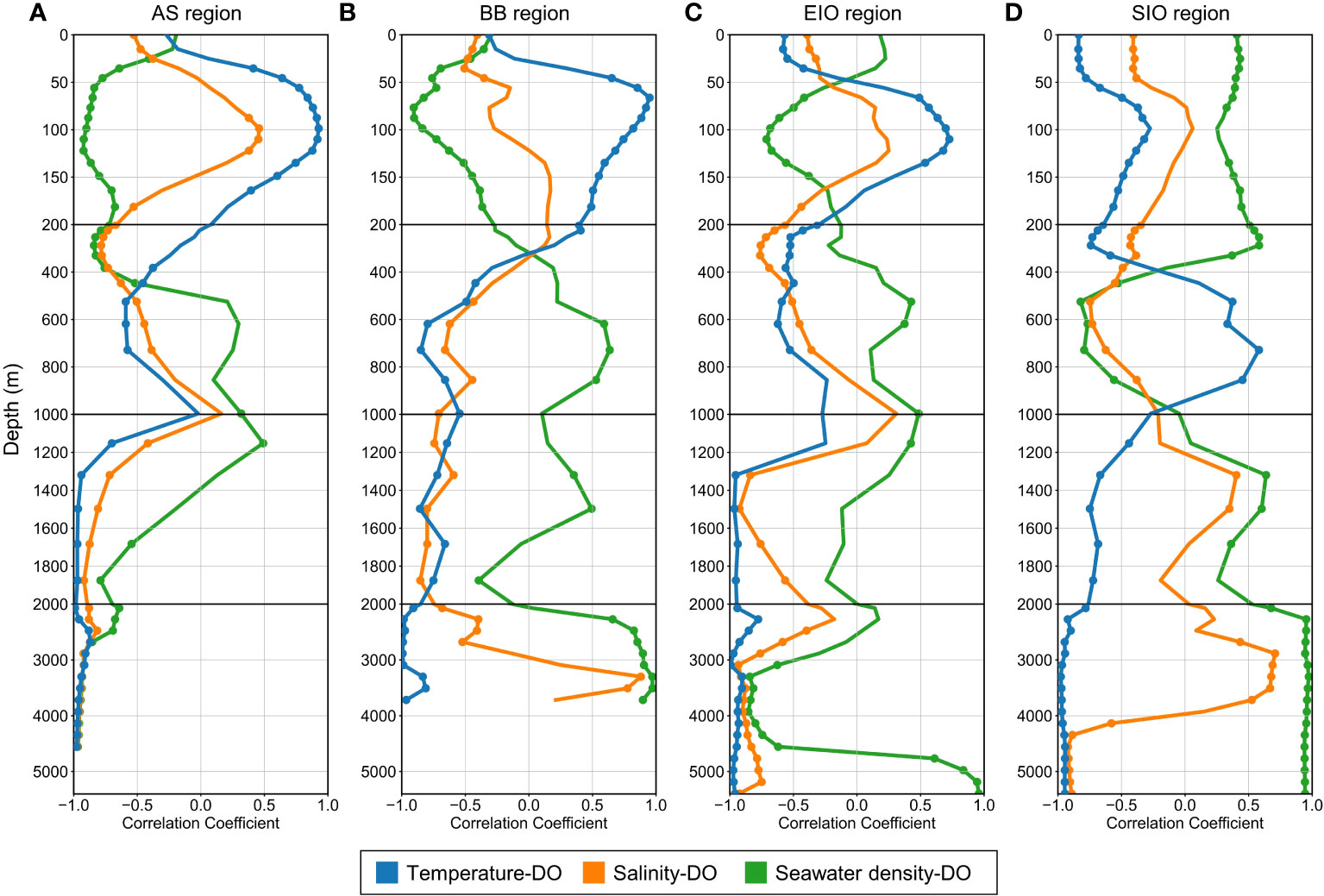
Figure 9 Correlation analysis between seawater temperature (blue lines), salinity (orange lines), potential density (green lines), and dissolved oxygen (DO) in the (A) Arabian Sea (AS), (B) Bay of Bengal (BB), (C) Equatorial Indian Ocean (EIO), and (D) Southern Indian Ocean (SIO). The blue, orange, and green scatter points represent that the correlations between seawater temperature, salinity, density, and DO within these depth layers are statistically significant at a 95% confidence level (p< 0.05), respectively.

In the upper 1,000 m of the AS, seawater temperature (trend = 0 to 0.1°C dec⁻¹) and salinity (trend = 0 to 0.05 psu dec⁻¹) have relatively small variations, but they still have complicated and heterogeneous correlations with DO concentration. At 0–200 m, DO has a mainly positive correlation with temperature (r = −0.27 to 0.93) but has different correlations with salinity (r = −0.53 to 0.46) and ocean currents (r = −0.60 to 0.40). DO variations may not be mainly caused by thermal factors, because temperature and salinity are not negatively correlated with DO as the oxygen solubility equation. At these regions, deoxygenation could be attributed to other factors such as biological consumption and remineralization. At 200–1,000 m, DO is mainly negatively correlated with temperature (r = −0.59 to 0.07) and salinity (r = −0.78 to 0.16), indicating that oxygen loss is controlled by the decreased solubility induced by warming. At 2,000 m–bottom, there are large increases in temperature (trend = 0.03 to 0.43°C dec⁻¹), salinity (trend = 0 to 0.12 psu dec⁻¹), and density (trend = 0 to 0.06 kg m⁻³ dec⁻¹). At these mid-depths, DO is highly negatively correlated with temperature (r = −0.99 to −0.87), salinity (r = −0.97 to −0.81), and density (r = −0.97 to −0.64). As a result, a rapid reduction in DO levels is strongly influenced by the combined effects of temperature and salinity variations, as well as enhanced stratification.

The deoxygenation situation in the EIO is similar to that of the AS, but DO variations in the EIO are relatively small compared to the AS. In the EIO at 0–200 m, DO has complex correlations with seawater temperature (r = −0.58 to 0.73), salinity (r = −0.44 to 0.25), and density (r = −0.71 to 0.22), indicating that this region has complex mechanisms of DO variations. Notably, the temperature trend is from increasing to decreasing at depths of 50–150 m, from which can be inferred that the EIO is not as strongly affected by ocean warming as the AS. At 200–1,000 m, DO has negative correlations with temperature (r = −0.62 to −0.24) and salinity (r = −0.76 to 0.31), and oxygen loss begins to be controlled by the increase of temperature (trend = 0.02 to 0.05°C dec⁻¹) and salinity (trend = 0 to 0.01 psu dec⁻¹). At 2,000 m–bottom, the variations of sea temperature (trend = 0 to 0.1°C dec⁻¹) and salinity (trend = 0 to 0.02 psu dec⁻¹) are still small, with coefficients ranging from −0.99 to −0.78 and −0.93 to 0.18, respectively. DO decline in these regions is strongly controlled by solubility, and other biological effects are weakened, leading to a significant decrease in solubility and DO loss.

5.1.2 Drivers of DO increase

The DO increasing regions are mainly located in the AS at 1,000–2,000 m, the BB at 40–80 m and 800–2500 m, the EIO at 1,000–2,000 m, and the SIO of 400–800 m. This section mainly analyzes the AS, BB, EIO, and SIO regions with increasing DO (Figures 8, 9, S4–S7).

Ocean conditions have similarities in the AS and EIO at depths of 1,000–2,000 m. At these water depths of sea regions, seawater temperature (AS trend = −0.05 to −0.02°C dec⁻¹, EIO trend = −0.02 to −0.01°C dec⁻¹) and salinity (AS trend = −0.02 to −0.01 psu dec⁻¹, EIO trend = 0 to −0.01 psu dec⁻¹) have decreased, and DO has strongly negative correlations with temperature (AS r = −0.97 to −0.70, EIO r = −0.96 to −0.25) and salinity (AS r = −0.92 to −0.42, EIO r = −0.92 to 0.08). In these regions, DO increase is mainly controlled by oxygen solubility, and a decrease in temperature and salinity causes an increase in DO solubility.

In the BB at 40–80 m and 800–2500 m, seawater temperature (upper trend = 0.05 to 0.15°C dec⁻¹, deeper trend = −0.02 to 0.05°C dec⁻¹) and salinity (upper trend = 0.02 psu dec⁻¹, deeper trend = 0 to −0.01 psu dec⁻¹) have increasing variations, and DO has different correlations with temperature (upper r = 0.65 to 0.95, deeper r = −0.98 to −0.54) and salinity (upper r = −0.35 to −0.15, deeper r = −0.85 to −0.40). In the SIO at 400–800 m, seawater temperature (trend = 0.04 to 0.05°C dec⁻¹) and salinity (trend = 0 to −0.01 psu dec⁻¹) have more slight variations, and DO has stable correlations with temperature (r = 0.11 to 0.58) and salinity (r = −0.75 to −0.55). It can be seen that the negative correlations between DO and sea temperature and salinity in those regions are weaker than the AS and EIO. Therefore, DO increases at these mid-depths are not only caused by solubility changes but also influenced by other DO supply mechanisms, such as vertical mixing and ocean circulation.

5.2 Change patterns of DO content

5.2.1 Spatiotemporal variations of DO content

In this section, we will mainly discuss the spatiotemporal variations of DO content in the Indian Ocean. We calculated the spatial distribution and trends of DO content (Figure 10) to analyze the spatial patterns of DO content. The spatial distribution of DO content in the Indian Ocean has the characteristics of being low in the north and high in the south, and changes transitionally along latitude, which is determined by ocean bathymetry and seawater volume. DO content in the AS and BB regions is relatively small, generally lower than 400 mol m⁻². However, DO content in the SIO is relatively large, and DO content in the southeast sea of Africa and the southwest sea of Australia can reach more than 1,000 mol m⁻². The greatest oxygen loss occurs in the AS, the western part of the EIO adjacent to the AS, and the southern African sea area, with DO loss up to 10 mol m⁻² dec⁻¹.

FIGURE 10

Figure 10 Spatial distribution, spatial trend, and time series of DO content at full depth of the Indian Ocean. (A) Spatial distribution and (B) spatial trend of DO content at full depth. Time series of DO content in the (C) Arabian Sea (AS), (D) Bay of Bengal (BB), (E) Equatorial Indian Ocean (EIO), (F) Southern Indian Ocean (SIO), and (G) total Indian Ocean regions. In (C–G), all DO content trends are statistically significant at a 95% confidence level (p < 0.01). The blue area surrounding the curve represents the uncertainty of oxygen, which is equal to twice the annual standard deviation of DO content, and the red dashed line represents the linear trend of DO content. In the BB, SIO, and total region, we used piecewise linear regression at a turning point of 2,000. (H) Time series of mean DO concentrations at 0–200 m, 200–1,000 m, 1,000–2,000 m, and 2,000 m–bottom. In (H), the solid curve represents the vertical mean DO concentration time series in different depth layers, and the bold dashed curve represents the full-depth mean DO concentration time series.

Furthermore, we calculated the entire DO content using volume integral, obtained the time series of DO content, and performed least square linear regression to estimate the trend of DO content in the Indian Ocean (Figure 10G) (the total trend and all the piecewise trends are statistically significant at a 95% confidence level). The result shows that the trend of total DO content is −141.5 ± 15.1 Tmol dec⁻¹, indicating that the Indian Ocean has lost −1.38 ± 0.15% oxygen from 1980 to 2019. We further used piecewise linear regression analysis on the time series of DO content and found that the change time of the DO trend appears around 2000 due to the DO content increasing from 2000 to 2010. Before 2000, DO content has a relatively large trend of −208.8 ± 25.9 Tmol dec⁻¹, while the trend decreases to −68.9 ± 31.3 Tmol dec⁻¹ after 2000.

To find out the cause of total DO content increasing, we compared the time series of DO content in subregions (Figures 10C–F) (the total trend and all the piecewise trends are statistically significant at a 95% confidence level). According to piecewise linear regression, DO content in the AS and EIO shows no significant trend change around 2000, and has a downward trend overall, which is −12.3 ± 2.5 Tmol dec⁻¹ and −45.1 ± 4.3 Tmol dec⁻¹, respectively. In contrast, DO content in the BB and SIO shows a time turning point around 2000, which is consistent with the change time of total DO. DO content in the BB decreased by −3.8 ± 1.2 Tmol dec⁻¹ in 1980–2000, and increased by 2.1 ± 1.3 Tmol dec⁻¹ in 2000–2019. DO content in the SIO decreased by −121.7 ± 21.7 Tmol dec⁻¹ in 1980–2000, and decreased by −41.4 ± 26.7 Tmol dec⁻¹ in 2000–2019. From the perspective of the order of magnitude, the expansion of DO content of the SIO from 2000 to 2010 resulted in the overall rise of the total DO content in the Indian Ocean, which can be attributed to the expansion of water bodies with high DO concentration at 200–1,000 m (Figure 6). The DO supply in the SIO has offset part of the oxygen loss in the Indian Ocean in the past 20 years, resulting in the DO decline trend slowing down.

Overall, the decline of oxygen in the Indian Ocean slowed down after the 2000s, with some sea areas experiencing oxygen increase. The upper 1,000-m circulation transports a substantial amount of oxygen-rich water, effectively mitigating the deterioration of the oxygen environment in the Indian Ocean. This suggests that the Indian Ocean may have a potential self-regulating mechanism against global warming.

5.2.2 Patterns of DO change rate

From the perspective of DO content, this section considers the trends of DO content at different depths in each sea region, and evaluates the oxygen change rates in different regions of the Indian Ocean. The mean oxygen change rate of the Indian Ocean is −0.59 ± 0.06 mmol m⁻³ dec⁻¹. We analyzed DO content anomalies in different layers (Figure 10H; Table 5) and found that the DO decline rate at depths of 0–200 m and 2,000 m–bottom is rapid, which is −1.10 ± 0.24 mmol m⁻³ dec⁻¹ and −0.69 ± 0.07 mmol m⁻³ dec⁻¹, respectively. Notably, DO content in the upper 200 m of the Indian Ocean is quite low due to the small ocean volumes, but oxygen decline rate in this region is extremely high.

TABLE 5

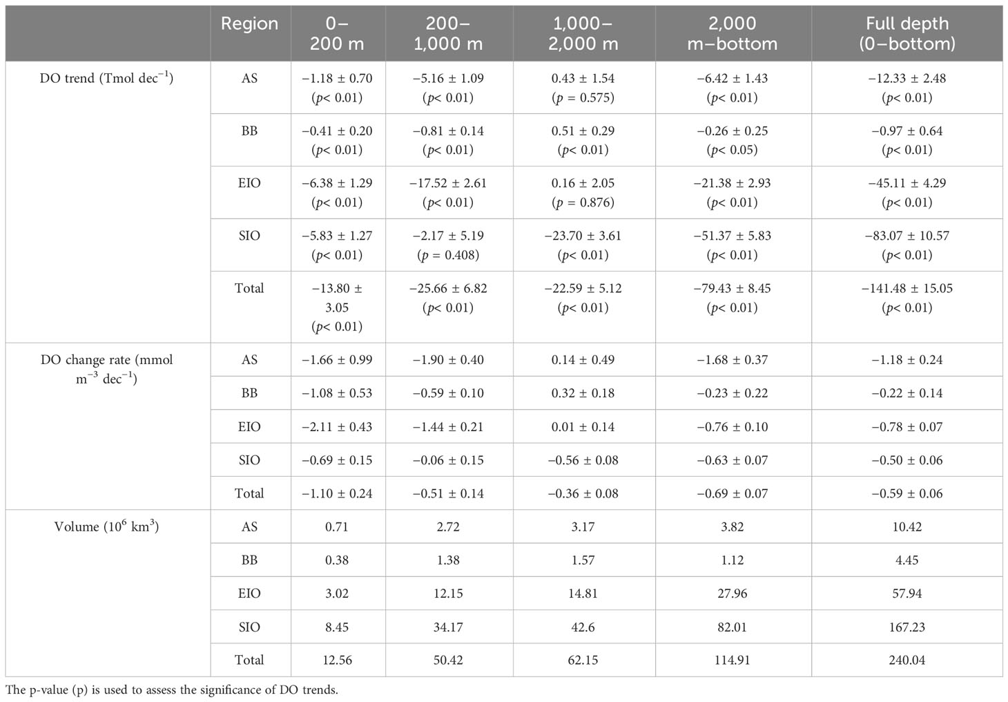
Table 5 The DO trend, DO change rate, and ocean volume in the Arabian Sea (AS), Bay of Bengal (BB), Equatorial Indian Ocean (EIO), Southern Indian Ocean (SIO), and total Indian Ocean at depths of 0–200 m, 200–1,000 m, 1,000–2,000 m, 2,000 m–bottom, and full depth during 1980–2019.

Considering the full depth of the water column, the oxygen decline rate ranking is AS > EIO > SIO > BB and the oxygen loss rates of the AS, BB, EIO, and SIO are −1.18 ± 0.24 mmol m⁻³ dec⁻¹, −0.22 ± 0.14 mmol m⁻³ dec⁻¹, −0.78 ± 0.07 mmol m⁻³ dec⁻¹, and −0.50 ± 0.06 mmol m⁻³ dec⁻¹, respectively. To compare spatiotemporal variations of DO in different regions, we calculated the DO change rates in different layers (Table 5). According to analysis of the results, the main deoxygenation regions are found in the AS at 0–1,000 m and 2,000 m–bottom, the BB at 0–200 m, and the EIO at 0–1,000 m with oxygen decline rates exceeding 1 mmol m⁻³ dec⁻¹, and oxygen-fixed regions are found at depths of 1,000–2,000 m in the AS, BB, and EIO.

We further compared our study with a previous study and found that our estimation for DO change in the Indian Ocean is consistent with the previous results (Schmidtko et al., 2017) in which the DO decline change rate of the EIO is greater than that of the SIO at full depth, and less than that of the SIO at depths of 1,000 m–bottom (Figure 11). Our study also found that the DO supply mechanism of the SIO at depths of 0–1,000 m was weakened, which resulted in a DO decline trend rather than an increasing trend like that during 1960–2010 in the SIO.

FIGURE 11

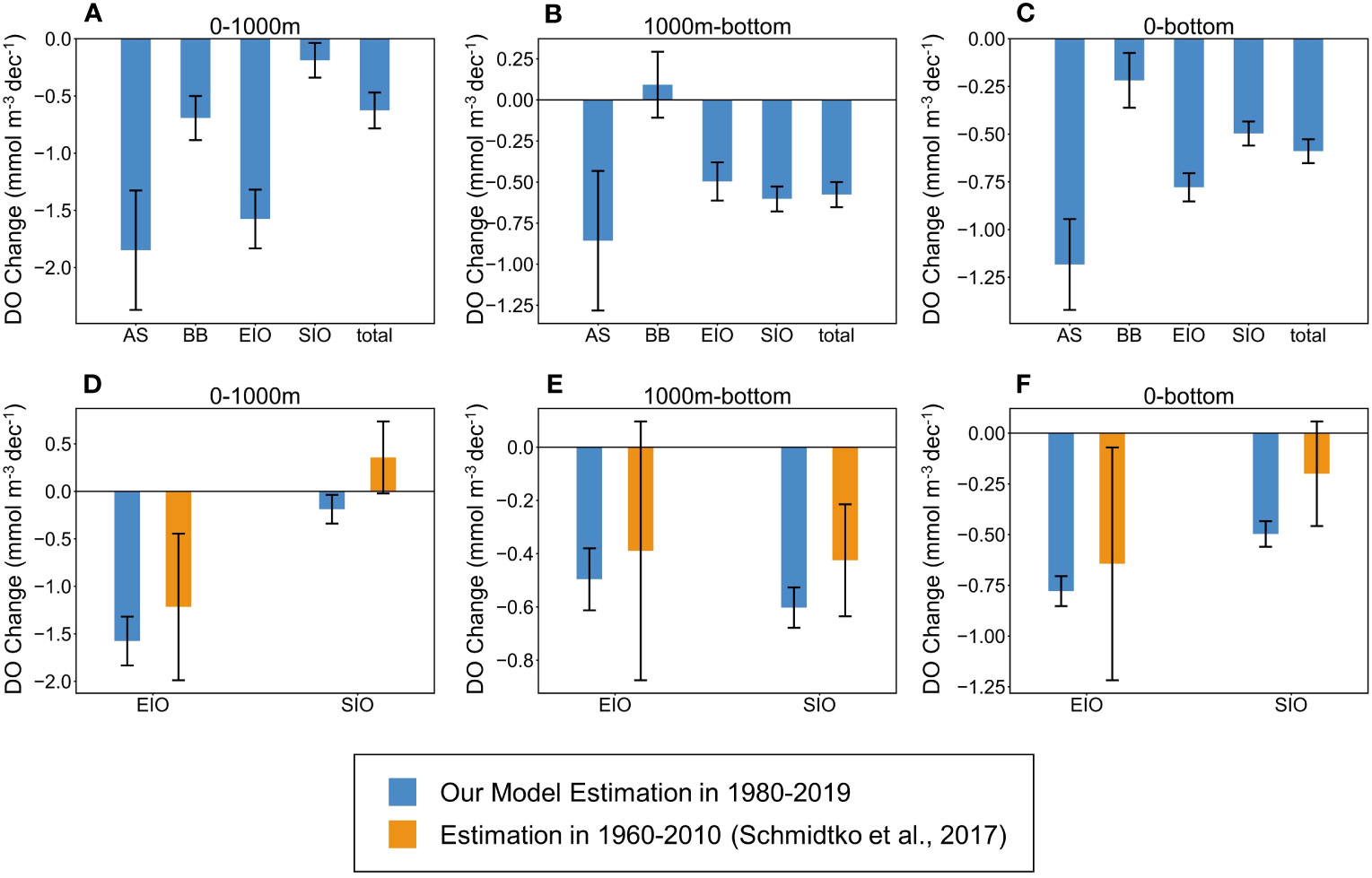
Figure 11 The DO change rates in the Indian Ocean. DO change rates of the Arabian Sea (AS), the Bay of Bengal (BB), the Equatorial Indian Ocean (EIO), Southern Indian Ocean (SIO), and the total regions (total) at depths of (A) 0–1,000 m, (B) 1,000 m–bottom, and (C) full depth. Comparison of DO change rates in 1980–2019 and 1960–2010 (Schmidtko et al., 2017) at depths of (D) 0–1,000 m, (E) 1,000 m–bottom, and (F) full depth.

6 Conclusion

In this study, we applied the ERT model to reconstruct DO in the Indian Ocean from 1980 to 2019 using a combination of measured DO observations, reanalysis data, and spatiotemporal information. Our evaluation shows that the reconstructed DO data have a high level of accuracy and are consistent with in situ observations, without abnormal overestimation or underestimation. Additionally, our results demonstrate that the spatiotemporal variation of our reconstructed DO data is more consistent with observations than the mean CMIP6 dataset.

We analyzed the spatiotemporal distribution of DO in the Indian Ocean using reconstructed data. DO concentration is higher in the SIO and lower in the AS and BB, with relatively high concentrations in the surface, subsurface, and deep waters and low concentrations in the thermocline. The OMZs in the Indian Ocean deteriorated, with the expansion of OMZ20 in the AS and BB and the emergence of OMZ60 in the EIO since the 1990s. DO decline regions are mainly located in the AS at 0–1,000 m and 2,000 m–bottom, the BB at 0–200 m, and the EIO at 0–1,000 m and 2,000 m–bottom. The deoxygenation is controlled by solubility reduction at mid-depths, and caused by other mechanisms at subsurface depths. DO increasing regions are located in the AS at 1,000–2,000 m, the BB at 40–80 m and 800–2500 m, the EIO at 1,000–2,000 m, and the SIO at 400–800 m. The rising DO is attributed to solubility increase (in the AS and EIO) and vertical mixing and circulation (in the BB and SIO). The complete time series of DO shows a trend of −141.5 ± 15.1 Tmol dec⁻¹ in 1980–2019, with a larger trend before 2000 and a lower trend after 2000. Since the beginning of the 21st century, the hypoxic areas and deoxygenation in the Indian Ocean have shown a slowdown trend, indicating that the Indian Ocean possesses a certain capacity to resist the deterioration of oxygen-depleted environments in the face of climate change.

Our findings of the long-term DO variations in the Indian Ocean could be beneficial for stakeholders and decision-makers working toward the conservation of marine organisms in this region. However, the contribution of remineralization, biological respiration, and ocean ventilation to DO changes is not fully investigated. Further efforts should focus on comprehensive research that examines the complex interactions among geographical factors, climate patterns, and oceanic processes to gain a deeper understanding of the drivers of DO changes. This knowledge with data-driven methods can then inform effective strategies for environmental management and conservation in the Indian Ocean, ensuring the preservation of this vital marine ecosystem for future generations.

Data availability statement

The raw data supporting the conclusions of this article will be made available by the authors, without undue reservation.

Author contributions

SH: Investigation, Methodology, Writing – original draft. JS: Data curation, Writing – review & editing. YC: Investigation, Validation, Writing – review & editing. JQ: Writing – review & editing. SW: Conceptualization, Methodology, Writing – review & editing. FZ: Writing – Review & editing. XH: Writing – review & editing. ZD: Funding acquisition, Project administration, Writing – review & editing.

Funding

The author(s) declare that financial support was received for the research, authorship, and/or publication of this article. This work was supported by the National Natural Science Foundation of China (grants 42225605, 42001323), National Key Research, Development Program of China (grant 2021YFB3900900), Provincial Key R&D Program of Zhejiang (grant 2021C01031), and Fundamental Research Funds for the Central Universities (2022FZZX01-05).

Acknowledgments

The authors thank three reviewers for their constructive suggestions. The authors extend their gratitude to the National Centers for Environmental Information in the National Oceanic and Atmospheric Administration for providing the WOD2018 data. The authors also appreciate The Ocean Climate Lab at the University of Maryland at College Park and the Asia-Pacific Data Research Center at the University of Hawaii at Mānoa for providing the SODA v3.4.2 data. Additionally, the authors acknowledge the World Climate Research Programme for providing the CMIP6 data. This work is also supported by the Deep-time Digital Earth (DDE) Big Science Program. The authors appreciate Professor Andreas Oschlies for his guidance on collecting measured oxygen data and determining the boundaries of the Indian Ocean. The authors appreciate Professor James T. Potemra for his guidance with utilizing and differentiation of SODA data. The authors are thankful to Dr. Hongjing Gong for her guidance on the long-term trend analysis of oxygen minimum zones and data visualization. The authors also express their gratitude to Professor Renguang Wu, Professor Long Cao, Professor Xiaojing Jia, Professor Cheng Su, Dr. Xiaoyan Chen, Dr. Qiwei Hu, Dr. Siqi Zhang, and Dr. Zhiyi Fu for their guidance in the development of ocean data-driven modeling. The generous support and guidance from the aforementioned researchers have significantly advanced the progress of this research.

Conflict of interest

The authors declare that the research was conducted in the absence of any commercial or financial relationships that could be construed as a potential conflict of interest.

Publisher’s note

All claims expressed in this article are solely those of the authors and do not necessarily represent those of their affiliated organizations, or those of the publisher, the editors and the reviewers. Any product that may be evaluated in this article, or claim that may be made by its manufacturer, is not guaranteed or endorsed by the publisher.

Supplementary material

The Supplementary Material for this article can be found online at: https://www.frontiersin.org/articles/10.3389/fmars.2023.1291232/full#supplementary-material

References

Amante C., Eakins B. W. (2009). ETOPO1 arc-minute global relief model: procedures, data sources and analysis. doi: 10.7289/V5C8276M

CrossRef Full Text | Google Scholar

Bopp L., Resplandy L., Orr J. C., Doney S. C., Dunne J. P., Gehlen M., et al. (2013). Multiple stressors of ocean ecosystems in the 21st century: projections with CMIP5 models. Biogeosciences 10 (10), 6225–6245. doi: 10.5194/bg-10-6225-2013

CrossRef Full Text | Google Scholar

Boyer T. P., Baranova O. K., Coleman C., Garcia H. E., Grodsky A., Locarnini R. A., et al. (2018). World ocean database 2018. A. V. Mishonov, Technical Editor, NOAA Atlas NESDIS 87. Available at: https://www.ncei.noaa.gov/sites/default/files/2020-04/wod_intro_0.pdf

Google Scholar

Breiman L. (2001). Random forests. Mach. Learn 45, 5–32. doi: 10.1023/A:1010933404324

CrossRef Full Text | Google Scholar

Breitburg D., Levin L. A., Oschlies A., Grégoire M., Chavez F. P., Conley D. J., et al. (2018). Declining oxygen in the global ocean and coastal waters. Science 359 (6371), eaam7240. doi: 10.1126/science.aam7240

PubMed Abstract | CrossRef Full Text | Google Scholar

Buchanan P. J., Tagliabue A. (2021). The regional importance of oxygen demand and supply for historical ocean oxygen trends. Geophys. Res. Lett. 48 (20), e2021GL094797. doi: 10.1029/2021GL094797

CrossRef Full Text | Google Scholar

Carton J. A., Chepurin G. A., Chen L. (2018). SODA3: A new ocean climate reanalysis. J. Climate 31 (17), 6967–6983. doi: 10.1175/JCLI-D-18-0149.1

CrossRef Full Text | Google Scholar

Cheng L., Trenberth K. E., Fasullo J., Boyer T., Abraham J., Zhu J., et al. (2017). Improved estimates of ocean heat content from 1960 to 2015. Sci. Adv. 3 (3), e1601545. doi: 10.1126/sciadv.1601545

PubMed Abstract | CrossRef Full Text | Google Scholar

Cocco V., Joos F., Steinacher M., Frölicher T. L., Bopp L., Dunne J., et al. (2013). Oxygen and indicators of stress for marine life in multi-model global warming projections. Biogeosciences 10 (3), 1849–1868. doi: 10.5194/bg-10-1849-2013

CrossRef Full Text | Google Scholar

Deutsch C., Brix H., Ito T., Frenzel H., Thompson L. (2011). Climate-forced variability of ocean hypoxia. Science 333 (6040), 336–339. doi: 10.1126/science.1202422

PubMed Abstract | CrossRef Full Text | Google Scholar

Dunne J. P., Horowitz L. W., Adcroft A. J., Ginoux P., Held I. M., John J. G., et al. (2020). The GFDL Earth System Model version 4.1 (GFDL-ESM 4.1): Overall coupled model description and simulation characteristics. J. Adv. Model. Earth Syst. 12 (11), e2019MS002015. doi: 10.1029/2019MS002015

CrossRef Full Text | Google Scholar

Freund Y., Schapire R. E. (1997). A decision-theoretic generalization of on-line learning and an application to boosting. J. Comput. Syst. Sci. 55 (1), 119–139. doi: 10.1006/jcss.1997.1504

CrossRef Full Text | Google Scholar

Friedman J. H. (2001). Greedy function approximation: a gradient boosting machine. Ann. Stat. 29 (5), 1189–1232. doi: 10.1214/aos/1013203451

CrossRef Full Text | Google Scholar

Garcia H. E., Gordon L. I. (1992). Oxygen solubility in seawater: Better fitting equations. Limnol. Oceanogr. 37, 1307–1312. doi: 10.4319/lo.1992.37.6.1307

CrossRef Full Text | Google Scholar

Garcia-Soto C., Cheng L., Caesar L., Schmidtko S., Jewett E. B., Cheripka A., et al. (2021). An overview of ocean climate change indicators: sea surface temperature, ocean heat content, ocean pH, dissolved oxygen concentration, Arctic Sea ice extent, thickness and volume, sea level and strength of the AMOC (Atlantic Meridional Overturning Circulation). Front. Mar. Sci. 8, 642372. doi: 10.3389/fmars.2021.642372

CrossRef Full Text | Google Scholar

Geurts P., Ernst D., Wehenkel L. (2006). Extremely randomized trees. Mach. Learn 63, 3–42. doi: 10.1007/s10994-006-6226-1

CrossRef Full Text | Google Scholar

Giglio D., Lyubchich V., Mazloff M. R. (2018). Estimating oxygen in the Southern Ocean using Argo temperature and salinity. J. Geophys. Res. Oceans 123 (6), 4280–4297. doi: 10.1029/2017JC013404

CrossRef Full Text | Google Scholar

Gruber N. (2011). Warming up, turning sour, losing breath: ocean biogeochemistry under global change, Philosophical Transactions of the Royal Society A: Mathematical. Phys. Eng. Sci. 369 (1943), 1980–1996. doi: 10.1098/rsta.2011.0003

CrossRef Full Text | Google Scholar

Helm K. P., Bindoff N. L., Church J. A. (2011). Observed decreases in oxygen content of the global ocean. Geophys. Res. Lett. 38 (23), n/a–n/a. doi: 10.1029/2011GL049513

CrossRef Full Text | Google Scholar

Irrgang C., Boers N., Sonnewald M., Barnes E. A., Kadow C., Staneva J., et al. (2021). Towards neural Earth system modelling by integrating artificial intelligence in Earth system science. Nat. Mach. Intell. 3 (8), 667–674. doi: 10.1038/s42256-021-00374-3

CrossRef Full Text | Google Scholar

Ito T., Minobe S., Long M. C., Deutsch C. (2017). Upper ocean O2 trends: 1958–2015. Geophys. Res. Lett. 44 (9), 4214–4223. doi: 10.1002/2017GL073613

CrossRef Full Text | Google Scholar

Keeling R. E., Körtzinger A., Gruber N. (2010). Ocean deoxygenation in a warming world. Annu. Rev. Mar. Sci. 2 (1), 199–229. doi: 10.1146/annurev.marine.010908.163855

CrossRef Full Text | Google Scholar

Kwiatkowski L., Torres O., Bopp L., Aumont O., Chamberlain M., Christian J. R., et al. (2020). Twenty-first century ocean warming, acidification, deoxygenation, and upper-ocean nutrient and primary production decline from CMIP6 model projections. Biogeosciences 17 (13), 3439–3470. doi: 10.5194/bg-17-3439-2020

CrossRef Full Text | Google Scholar

Lachkar Z., Lévy M., Smith S. (2018). Intensification and deepening of the Arabian Sea oxygen minimum zone in response to increase in Indian monsoon wind intensity. Biogeosciences 15 (1), 159–186. doi: 10.5194/bg-15-159-2018

CrossRef Full Text | Google Scholar

Lachkar Z., Lévy M., Smith K. S. (2019). Strong intensification of the arabian sea oxygen minimum zone in response to arabian gulf warming. Geophys. Res. Lett. 46 (10), 5420–5429. doi: 10.1029/2018GL081631

CrossRef Full Text | Google Scholar

LeCun Y., Bengio Y., Hinton G. (2015). Deep learning. Nature 521 (7553), 436–444. doi: 10.1038/nature14539

PubMed Abstract | CrossRef Full Text | Google Scholar

Levin L. A. (2018). Manifestation, drivers, and emergence of open ocean deoxygenation. Annu. Rev. Mar. Sci. 10 (1), 229–260. doi: 10.1146/annurev-marine-121916-063359

CrossRef Full Text | Google Scholar

Li G., Cheng L., Zhu J., Trenberth K. E., Mann M. E., Abraham J. P. (2020). Increasing ocean stratification over the past half-century. Nat. Clim. Change 10 (12), 1116–1123. doi: 10.1038/s41558-020-00918-2

CrossRef Full Text | Google Scholar

Long M. C., Deutsch C., Ito T. (2016). Finding forced trends in oceanic oxygen. Global Biogeochem. Cycles 30 (2), 381–397. doi: 10.1002/2015GB005310

CrossRef Full Text | Google Scholar

Lovato T., Peano D., Butenschön M., Materia S., Iovino D., Scoccimarro E., et al. (2022). CMIP6 simulations with the CMCC earth system model (CMCC-ESM2). J. Adv. Model. Earth Syst. 14 (3), e2021MS002814. doi: 10.1029/2021MS002814

CrossRef Full Text | Google Scholar

Mauritsen T., Bader J., Becker T., Behrens J., Bittner M., Brokopf R., et al. (2019). Developments in the MPI-M Earth System Model version 1.2 (MPI-ESM1. 2) and its response to increasing CO2. J. Adv. Model. Earth Syst. 11 (4), 998–1038. doi: 10.1029/2018MS001400

PubMed Abstract | CrossRef Full Text | Google Scholar

McCreary J. P., Yu Z., Hood R. R., Vinaychandran P. N., Furue R., Ishida A., et al. (2013). Dynamics of the Indian-Ocean oxygen minimum zones. Prog. Oceanogr. 112-113, 15–37. doi: 10.1016/j.pocean.2013.03.002

CrossRef Full Text | Google Scholar

Naqvi S. W. A. (2021). Deoxygenation in marginal seas of the Indian ocean. Front. Mar. Sci. 8, 624322. doi: 10.3389/fmars.2021.624322

CrossRef Full Text | Google Scholar

Oschlies A., Brandt P., Stramma L., Schmidtko S. (2018). Drivers and mechanisms of ocean deoxygenation. Nat. Geosci 11 (7), 467–473. doi: 10.1038/s41561-018-0152-2

CrossRef Full Text | Google Scholar

Portela E., Kolodziejczyk N., Vic C., Thierry V. (2020). Physical mechanisms driving oxygen subduction in the global ocean. Geophys. Res. Lett. 47 (17), e2020GL089040. doi: 10.1029/2020GL089040

CrossRef Full Text | Google Scholar

Reichstein M., Camps-Valls G., Stevens B., Jung M., Denzler J., Carvalhais N., et al. (2019). Deep learning and process understanding for data-driven Earth system science. Nature 566 (7743), 195–204. doi: 10.1038/s41586-019-0912-1

PubMed Abstract | CrossRef Full Text | Google Scholar

Reiniger R. F., Ross C. K. (1968). “A method of interpolation with application to oceanographic data.” in Deep Sea Research and Oceanographic Abstracts (Elsevier), 185–193. doi: 10.1016/0011-7471(68)90040-5

CrossRef Full Text | Google Scholar

Rixen T., Cowie G., Gaye B., Goes J., Do Rosario Gomes H., Hood R. R., et al. (2020). Reviews and syntheses: Present, past, and future of the oxygen minimum zone in the northern Indian Ocean. Biogeosciences 17 (23), 6051–6080. doi: 10.5194/bg-17-6051-2020

CrossRef Full Text | Google Scholar

Roxy M. K., Ritika K., Terray P., Masson S. (2014). The curious case of Indian ocean warming. J. Climate 27 (22), 8501–8509. doi: 10.1175/JCLI-D-14-00471.1

CrossRef Full Text | Google Scholar

Sadaiappan B., Balakrishnan P. C. R. V., Vijayan N. T., Subramanian M., Gauns M. U. (2023). Applications of machine learning in chemical and biological oceanography. ACS Omega 8 (18), 15831–15853. doi: 10.1021/acsomega.2c06441

PubMed Abstract | CrossRef Full Text | Google Scholar

Sallée J., Pellichero V., Akhoudas C., Pauthenet E., Vignes L., Schmidtko S., et al. (2021). Summertime increases in upper-ocean stratification and mixed-layer depth. Nature 591 (7851), 592–598. doi: 10.1038/s41586-021-03303-x

PubMed Abstract | CrossRef Full Text | Google Scholar

Santer B. D., Wigley T. M. L., Boyle J. S., Gaffen D. J., Hnilo J. J., Nychka D., et al. (2000). Statistical significance of trends and trend differences in layer-average atmospheric temperature time series. J. Geophys. Res. Atmospheres 105 (D6), 7337–7356. doi: 10.1029/1999JD901105

CrossRef Full Text | Google Scholar

Sarma V. V. S. S., Bhaskar T. V. S. U., Kumar J. P., Chakraborty K. (2020). Potential mechanisms responsible for occurrence of core oxygen minimum zone in the north-eastern Arabian Sea. Deep Sea Res. Part I: Oceanographic Res. Papers 165, 103393. doi: 10.1016/j.dsr.2020.103393

CrossRef Full Text | Google Scholar

Sarma V. V. S. S., Krishna M. S., Viswanadham R., Rao G. D., Rao V. D., Sridevi B., et al. (2013). Intensified oxygen minimum zone on the western shelf of Bay of Bengal during summer monsoon: influence of river discharge. J. Oceanogr. 69 (1), 45–55. doi: 10.1007/s10872-012-0156-2

CrossRef Full Text | Google Scholar

Schmidtko S., Stramma L., Visbeck M. (2017). Decline in global oceanic oxygen content during the past five decades. Nature 542 (7641), 335–339. doi: 10.1038/nature21399

PubMed Abstract | CrossRef Full Text | Google Scholar

Séférian R., Nabat P., Michou M., Saint Martin D., Voldoire A., Colin J., et al. (2019). Evaluation of CNRM Earth System Model, CNRM-ESM2-1: Role of Earth system processes in present-day and future climate. J. Adv. Model. Earth Syst. 11 (12), 4182–4227. doi: 10.1029/2019MS001791

CrossRef Full Text | Google Scholar

Sharp J. D., Fassbender A. J., Carter B. R., Johnson G. C., Schultz C., Dunne J. P. (2023). GOBAI-O2: temporally and spatially resolved fields of ocean interior dissolved oxygen over nearly 2 decades. Earth Syst. Sci. Data 15 (10), 4481–4518. doi: 10.5194/essd-15-4481-2023

CrossRef Full Text | Google Scholar

Stramma L., Johnson G. C., Sprintall J., Mohrholz V. (2008). Expanding oxygen-minimum zones in the tropical oceans. Science 320 (5876), 655–658. doi: 10.1126/science.1153847

PubMed Abstract | CrossRef Full Text | Google Scholar

Stramma L., Prince E. D., Schmidtko S., Luo J., Hoolihan J. P., Visbeck M., et al. (2012). Expansion of oxygen minimum zones may reduce available habitat for tropical pelagic fishes. Nat. Clim. Change 2 (1), 33–37. doi: 10.1038/nclimate1304

CrossRef Full Text | Google Scholar

Stramma L., Schmidtko S., Levin L. A., Johnson G. C. (2010). Ocean oxygen minima expansions and their biological impacts. Deep Sea Res. Part I: Oceanographic Res. Papers 57 (4), 587–595. doi: 10.1016/j.dsr.2010.01.005

CrossRef Full Text | Google Scholar

Swart N. C., Cole J. N. S., Kharin V. V., Lazare M., Scinocca J. F., Gillett N. P., et al. (2019). The canadian earth system model version 5 (CanESM5.0.3). Geosci. Model. Dev. 12 (11), 4823–4873. doi: 10.5194/gmd-12-4823-2019

CrossRef Full Text | Google Scholar

Vaquer-Sunyer R., Duarte C. M. (2008). Thresholds of hypoxia for marine biodiversity. Proc. Natl. Acad. Sci. 105 (40), 15452–15457. doi: 10.1073/pnas.0803833105

CrossRef Full Text | Google Scholar

Zhou Y., Gong H., Zhou F. (2022). Responses of horizontally expanding oceanic oxygen minimum zones to climate change based on observations. Geophys. Res. Lett. 49 (6), n/a–n/a. doi: 10.1029/2022GL097724

CrossRef Full Text | Google Scholar

Ziehn T., Chamberlain M. A., Law R. M., Lenton A., Bodman R. W., Dix M., et al. (2020). The Australian earth system model: ACCESS-ESM1.5. J. South. Hemisphere Earth Syst. Sci. 70 (1), 193–214. doi: 10.1071/ES19035

CrossRef Full Text | Google Scholar