A method for estimating particulate organic carbon at the sea surface based on geodetector and machine learning

1 Introduction

Marine particulate organic carbon (POC) refers to the organic particles in the ocean that are generated through the metabolic processes of marine organisms, resuspension of sediments, and input from land sources. These particles include phytoplankton cells, bacteria, and organic debris, among other substances (Brewin et al., 2021). POC accounts for approximately 10% of ocean organic carbon reservoirs (Jahnke and Richard, 1996; Loisel et al., 2002). Although POC accounts for a small proportion of the open ocean, it is an essential component of biological pumps with a high carbon turnover rate and significant carbon flux (Sarmiento, 2006; Kim et al., 2022; Lao et al., 2023a). Therefore, analyzing spatiotemporal variations in the stock and flux of POC in the ocean is of great significance for studying the marine carbon cycle. Remote sensing data offer significant advantages in terms of temporal and spatial resolution (Sawaya et al., 2003; Devi et al., 2015). By utilizing remote sensing techniques, it is possible to provide additional methods for estimating the POC stock in the ocean (Stramski et al., 1999). POC does not possess optical activity, making it challenging to directly retrieve POC information from remote sensing signals (Wang et al., 2017). Researchers, both domestically and internationally, have conducted a series of studies on the factors influencing POC and found correlations between POC and inherent optical properties (IOPs), apparent optical properties (AOPs), and water constituents (Stramski et al., 1999; Stramski et al., 2008). Based on these findings, scientists proposed a range of POC retrieval algorithms.

Stramski et al. (1999) were the first to estimate the distribution of POC using the IOPs of water. Based on measured POC data, they established an empirical relationship between POC and the particle backscattering coefficient (bbp). This relationship was then used to quantitatively estimate POC concentrations in the Southern Ocean (Stramski et al., 1999). Loisel et al. (2001) discovered a near-linear relationship between POC and bbp in the Southern Ocean. Based on this relationship, they derived the global spatial distribution and seasonal variations of POC using bbp (Loisel et al., 2001). According to the measured POC data, Gardner et al. (2006) established an empirical relationship between the particle attenuation coefficient (cp) and POC. Using this relationship, they developed a Two-Step algorithm (Gardner et al., 2006). However, accurately deducing IOPs from AOPs is crucial for a POC retrieval model based on IOPs (Jiang et al., 2015; Hayley et al., 2017; Liu et al., 2021).

In addition, some algorithms directly estimate POC based on AOPs. For instance, Stramski et al. (2008) proposed a blue-to-green band ratio algorithm based on the relationship between POC concentrations and remote sensing reflectance (Rrs) in the blue and green bands (Stramski et al., 2008). Currently, the NASA standard POC algorithm belongs to this category. O'Reilly and Werdell (2019) proposed a maximum band ratio-OCx (MBR-OCx) algorithm for chlorophyll estimation. Stramski et al. (2022) tested the performance of the Maximum Band Ratio for POC estimation (O'Reilly, 2000; O'Reilly and Werdell, 2019; Stramski et al., 2022). Le et al. (2017) established a POC estimation method using a color index (CI) based on satellite Rrs data and matched POC measurements (Le et al., 2017). Son et al. (2009) proposed the estimation of POC using the normalized difference carbon index (NDCI) inspired by the normalized difference vegetation index. The results showed high accuracy (R² = 0.97, N=58). Furthermore, Son et al. (2009) introduced the maximum normalized difference carbon index (MNDCI) based on the NDCI, demonstrating even higher accuracy than the previous NDCI (Son et al., 2009; Wang et al., 2017). The algorithms mentioned above are suitable for open-ocean Type I waters, whereas the others are more suitable for coastal Type II waters (Morel and Prieur, 1977). Several scholars have comprehensively tested the algorithms above and developed a series of hybrid algorithms. Stramski et al. (2022) combined the band ratio difference index (BRDI) algorithm with the MBR-OC4 algorithm based on POC concentration. The final hybrid algorithm achieved good accuracy in both Type I and Type II waters, significantly improving the universality of POC estimation algorithms. Cai et al. (2022) developed a hybrid algorithm for the East China Sea based on the CI and band ratio algorithms. Using this algorithm, they conducted a long-term time-series estimation and achieved satisfactory accuracy (Cai et al., 2022; Stramski et al., 2022).

Owing to the improved fitting capability of machine learning for nonlinear data, its application in water color remote sensing has become increasingly widespread. Scholars have already explored the use of machine learning methods for estimating POC. Liu et al. (2021) trained three machine learning models: extreme gradient boosting (XGBoost), support vector machine (SVM), and Artificial Neural Networks (ANN). They compared these models with the traditional blue-to-green band ratio algorithm for POC estimation. The results showed that the performance of the machine learning algorithms was superior to that of traditional algorithms. Additionally, machine learning algorithms better estimate the POC in marginal seas and optically complex estuarine waters (Liu et al., 2021). Sauzède et al. (2016) developed the “Satellite Ocean-Color merged with Argo data to infer bio-optical properties to depth” (SOCA) method, a neural network-based method trained using the Biogeochemical-Argo database, for estimating the vertical distribution of bbp. SOCA was improved by Sauzède et al. (2020), and the new SOCA2020 model improved the accuracy of POC estimation and additionally estimated chlorophyll-a (Sauzède et al., 2021; Sauzède et al., 2020). However, owing to the complex optical conditions in coastal areas, the distribution of POC exhibits significant spatial heterogeneity, which results in uncertainty in POC estimation, even when using machine learning methods.

Geodetector is a novel statistical method for detecting spatial heterogeneity and identifying the underlying driving factors. This approach does not assume linearity and can be used to measure spatial differentiation, detect explanatory factors, or analyze the interactions between variables. It has been applied in various fields of the natural and social sciences (Wang and Xu, 2017). In this study, to improve the performance of machine learning in estimating the global ocean POC, geodetector was used to detect the spatial correlation between POC and 30 factors. Six machine learning models were trained: backpropagation neural network (BPNN), convolutional neural network (CNN), attention-based neural network (ABNN), random forest (RF), adaptive boosting (AdaBoost), and extreme gradient boosting (XGBoost). The performances of these models were compared and evaluated. This study estimated the annual average surface POC concentration globally from 2007 to 2017 and compared it with NASA’s POC product. This study contributes to the development of global high-precision POC products by addressing the uncertainty caused by the significant spatial heterogeneity of POC in coastal areas.

2 Materials and methods

2.1 In situ data

This study utilized data from three publicly available datasets: 1) The NASA Bio-Optical Marine Algorithm Dataset, which is a global, high-quality dataset for in situ bio-optical measurements; it is used to develop ocean color algorithms and validate satellite products (Werdell and Bailey, 2005). 2) The SeaWiFS Bio-optical Archive and Storage System (SeaBASS) website (https://seabass.gsfc.nasa.gov/) provides access to the in situ POC measurement data. SeaBASS is an oceanic and atmospheric measurement database maintained by the NASA Ocean Biology Processing Group; it collects in situ measurement data from various global cruise missions and observation sites (Werdell and Bailey, 2005). 3) Martiny et al. (2014) collected 60,811 in situ data points from 70 global cruise missions (Martiny et al., 2014). To establish a global surface POC estimation model in their study, the downloaded POC data were standardized, and data at depths of less than 20 m were retained as shallow surface POC concentrations. In cases where multiple measurements were available for the same spatiotemporal coordinates, the average value was considered the measured POC value for that particular point. In total, 21,955 surface POC data points were obtained.

2.2 Matching of satellite and reanalysis data with in situ data

Moderate Resolution Imaging Spectroradiometer (MODIS) data was downloaded from the NASA OCEAN COLOR website (https://oceancolor.gsfc.nasa.gov/), and remote sensing reanalysis data from multiple databases downloaded from the Copernicus Marine Service (https://marine.copernicus.eu/) (Lavergne et al., 2019; Merchant et al., 2019; Good et al., 2020). The statistical information on the remote sensing and reanalysis data is presented in Supplementary Table S1. According to the collected in situ POC measurement data, remote sensing, and reanalysis data covering 2007 to 2017 were used. The temporal resolution was standardized at monthly intervals. The ArcGIS mapping tool was used to match the POC measurement data with satellite data using a monthly time window, which reduces the time lag in the correlation between POC and influencing factors and improves the stability of the matching results (Bonelli et al., 2022). Finally, 14,067 matched points were obtained for the 2007–2017 period. The geographic distribution of the matching points is shown in Figure 1. The maximum POC concentration observed was 4743 mg/m³, the minimum was 1.45 mg/m³, and the average was 156.59 mg/m³.

Figure 1

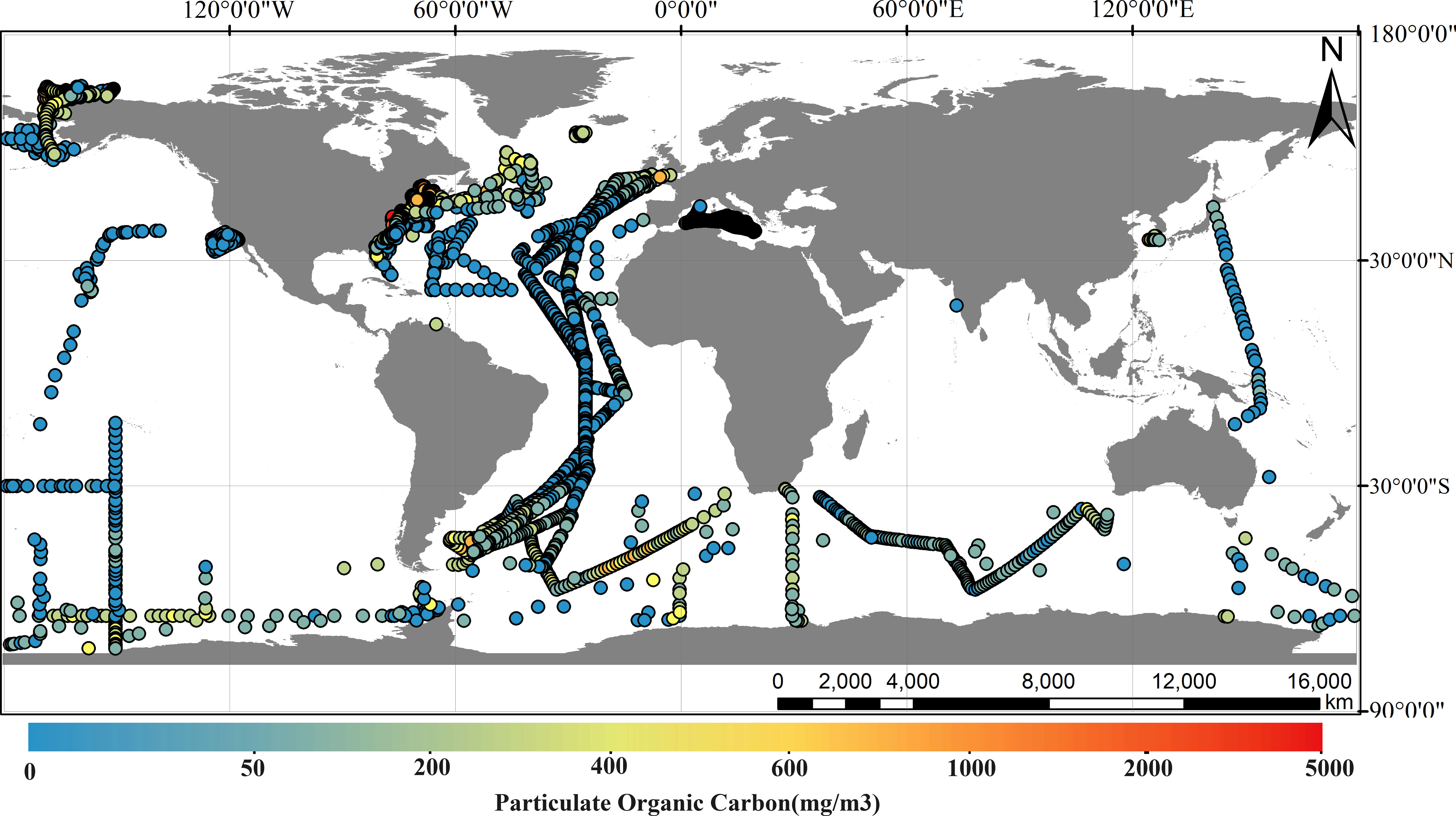
Figure 1 Geographic distribution of matching points for particulate organic carbon (POC) and remote sensing data, where the color of the point represents the magnitude of the POC concentration.

2.3 Dataset segmentation

Suspended particulate matter (SPM) refers to the solid particles suspended in water, including organic and inorganic particles. Therefore, the ratio of POC to SPM (POC/SPM) can be used to measure the contribution of organic particles to total suspended particles (Stramski et al., 2008; Woźniak et al., 2010; Tran et al., 2019). According to the POC/SPM ratio, waters can be classified into three types (Woźniak et al., 2010): if POC/SPM< 0.06, the particles in the water are predominantly mineral-based; if POC/SPM > 0.25, the particles in the water are predominantly organic-based; if 0.06< POC/SPM< 0.25, it is considered a mixed water. This study compiled the POC concentration ranges for the three types of waters in the dataset, as shown in Table 1 and illustrated in the box plot in Figure 2.

Table 1

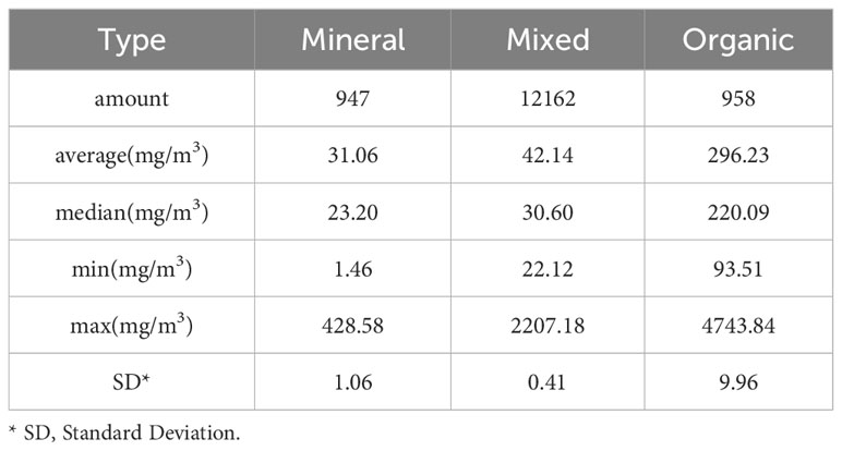
Table 1 Statistical data table of measured points for mineral, organic, and mixed water.

Figure 2

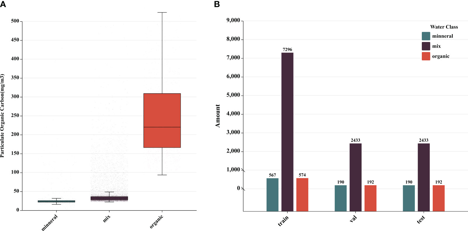
Figure 2 (A) Statistics of the particulate organic carbon concentration ranges of organic water, mineral water, and mixed water in the dataset; (B) Statistics of the number of measured data belonging to the three types of waters in the training, validation, and test datasets.

As shown in Table 1, there were 947 observations of mineral water type in the dataset, with an average POC concentration of 31.06 mg/m³ and a median of 23.20 mg/m³. For the mixed water type, there were 12,162 observations with an average POC concentration of 42.14 mg/m³ and a median of 30.60 mg/m³. Finally, for the organic water type, there were 958 observations with an average POC concentration of 296.23 mg/m³ and a median of 220.09 mg/m³. The standard error of POC for all three water types was less than 10 mg/m³, indicating a relatively concentrated distribution of data within each group. From Figure 2, it is evident that there are significant differences among the three groups. Thus, using POC/SPM as a classification criterion for waters effectively represented the differences in POC concentrations within this research dataset.

The dataset was divided into three parts according to the water type to train and evaluate the machine learning model. Each part was further split into training, validation, and test datasets at a ratio of 6:2:2, as shown in Figure 2. The resulting dataset contained approximately equal proportions of the three water types, with distributions of approximately 7% mineral, 86% mixed, and 7% organic water. This data partitioning method ensures that the POC measured data in the training, validation, and test datasets have similar distribution patterns, which can enhance the effectiveness of the subsequent machine learning model training and evaluation.

2.4 Feature selection method

The objective of feature selection is to find the features most relevant to the target variable while excluding those that do not contribute to the model’s performance. This is an important step in machine learning that helps reduce data redundancy and noise and improves the model’s generalization and interpretability (Liu et al., 2021). Geodetector was employed to select features for the model. Its theoretical foundation is spatial autocorrelation, which breaks the assumption of independent and identically distributed data in classical statistics (Elhorst, 2010). The core idea is that if an independent variable significantly influences a dependent variable, the spatial distribution of the independent variable should be similar to that of the dependent variable (Wang and Hu, 2012). Geodetector is adept at analyzing categorical variables, and for ordinal, ratio, or interval variables, they can also be subjected to appropriate discretization for statistical analysis using geodetector (Cao et al., 2013). Geodetector consist of four detectors, where the q-value in factor detection represents the extent to which factor explains the spatial variation in attribute POC. The formula used is as Equation 1:

$\begin{array}{ll}\text{q}=1-\frac{WSS}{\text{TSS}}& (1)\end{array}$

In the equation, WSS represents the within sum of squares, and TSS represents the total sum of squares. Interaction detection assesses whether the interaction between two factors increases or decreases the explanatory power of the dependent variable or whether the effects of these factors on POC are independent of each other.

The spatial distribution of POC at a global scale is uneven. This study utilized geodetector analysis to identify the factors influencing POC concentration, ensuring that the spatial distribution of each factor is similar to that of POC. By validating the spatial correlation between each factor and POC, the model can better represent the spatial distribution characteristics of POC.

2.5 Machine learning methods

Six machine learning models were trained in this study, including the BPNN, CNN, ABNN, RF, AdaBoost, and XGBoost, to estimate POC on the ocean surface. The performance of each model was tested individually.

ANN consist of a complex network structure that includes an input layer, hidden layer(s), and an output layer (Mcculloch and Pitts, 1990). The ANN learns and adapts to tasks through continuous training and weights (Lecun et al., 2015). Popular training algorithms for ANN include backpropagation and gradient descent algorithms. This study’s BPNN model consisted of one input layer, ten hidden layers, and one output layer. The first hidden layer contained 89 neurons, and the remaining hidden layers contained 52 neurons. The activation function used between the input and hidden layers and between the output and hidden layers is ReLU. The mean squared error (MSE) was used as a loss function to train the model.

CNN is widely used in image recognition and computer vision tasks. Compared with traditional fully connected neural networks, CNNs have the characteristics of local connectivity and weight sharing, which enable them to effectively extract spatial features from images (Lecun et al., 1998). The core components of a CNN are the convolutional and pooling layers. The CNN model used in this study consisted of a one-dimensional convolutional layer with one input channel, 16 output channels, and three convolutional kernels. It also included a fully connected layer and an output layer. The ReLU activation function was applied to the nonlinear transformations between each layer. The MSE was used as a loss function to train the model.

The ABNN enhances the model’s performance for specific tasks by introducing attention mechanisms; it can automatically learn and select important features from input data and model their correlations using a special weight allocation method (Yang et al., 2019). In this study, we first used fully connected layers for the feature transformation. The softmax function was used to calculate attention weights, which were used to weigh the features. The weighted features were summed. Similarly, the ReLU activation function was used for nonlinear transformations between layers.

AdaBoost builds a robust classifier by combining multiple weak classifiers, such as decision stumps (decision trees with only one split node) or simple linear classifiers. One characteristic of AdaBoost is that in each training round, it assigns higher weights to samples misclassified in the previous round. This allows weak classifiers to focus on misclassified samples, improving their overall performance and robustness (Freund and Schapire, 1995). This study used the sklearn library for python to build Adaboost. Decision trees were used as weak regressors, and the total number of iterations in the ensemble was set to 100.

XGBoost is an ensemble learning method based on a gradient-boosting algorithm used to solve classification and regression problems. This is an extension of the boosting algorithm and is known for its efficiency and accuracy, making it widely applicable across various domains. In the context of quantitative watercolor remote sensing, XGBoost is primarily used to predict and estimate water quality parameters of water (Krishnapuram et al., 2016; Massari et al., 2018; Zou et al., 2021). In this study, we implemented XGBoost using sklearn library for python with 100 decision trees in the ensemble and a 0.1 learning rate.

Random Forest (RF) is also an ensemble learning algorithm that combines multiple decision trees for classification and regression. This improves the robustness and generalizability of the model by utilizing random sampling and feature selection to combine multiple decision trees (Breiman, 2001; Verde et al., 2018; Shi et al., 2019).

2.6 Statistical indicators used for model development, validation and test

This research model performance assessment metrics include coefficient of determination (R2), root mean square error (RMSE), mean absolute percentage error (MAPE), bias, and variance.

R² is a statistical measure used to assess the degree to which a model fits the data. The formula is as Equation 2:

$\begin{array}{ll}{R}^2=1-\frac{SSR}{SS}& (2)\end{array}$

SSR represents the sum of squares due to regression, and SS represents the sum of squares.

The RMSE is a statistical measure that assesses the error between predicted and true values in a model. The calculation formula is as Equation 3:

$\begin{array}{ll}RMSE=\sqrt{(\frac{1}{n}\times {\displaystyle \sum {(PO{C}_{pred}-PO{C}_{true})}^2})}& (3)\end{array}$

The MAPE is a statistical measure that assesses the average relative error between a model’s predicted and true values. The formula is as Equation 4:

$\begin{array}{ll}MAPE=\frac{1}{n}\times {\displaystyle \sum (\left|\frac{PO{C}_{pred}-PO{C}_{true}}{PO{C}_{true}}\right|)}\times 100& (4)\end{array}$

Bias measured the overall error direction of the model. Variance measures the sensitivity and volatility of the model to the samples. The formulas for the bias and variance are as Equations 5, 6:

$\begin{array}{ll}Bias=\frac{1}{n}\times {\displaystyle \sum (PO{C}_{pred}-PO{C}_{true})}& (5)\end{array}$

$\begin{array}{ll}Variance=\frac{1}{n}\times {\displaystyle \sum {(PO{C}_{pred}-PO{C}_{mean})}^2}& (6)\end{array}$

In the formulas above, n represents the number of samples, POC_pred represents the model’s predicted value, POC_true represents the true value, POC_mean represents the mean predicted value, and Σ denotes the summation.

3 Results and discussion

3.1 Feature selection

This study utilized factor and interaction detection in a geodetector to select features for pre-model training. The candidate features can be divided into three parts.

The first part comprises the apparent optical properties (AOPs) and their mathematical combination. The AOPs is a product of the interaction between the incident light flux inside the water and the intrinsic optical properties of the water, which varies with the distribution and intensity of the incident light field. These quantities include downward irradiance (Ed), upward irradiance (Eu), water-leaving radiance (LW), Rrs, and the diffuse attenuation coefficients of these variables (Zaneveld and Mobley, 1995). In this study, the diffuse attenuation coefficient (kd) at 490 nm from the MODIS sensor was collected, as well as the Rrs at wavelengths of 412 nm, 443 nm, 469 nm, 488 nm, 547 nm, 555 nm, 645 nm, and 667 nm. This encompassed the wavelength ranges of red, green, and blue light. Based on the AOPs (mainly Rrs), this study combined band ratios (red-green, red-blue, and blue-green), normalized difference carbon index (NDCI), color index (CI), and band ratio difference index (BRDI) as candidate features.

The second part consists of Inherent optical properties (IOPs), which are solely related to the internal composition of water and do not vary with changing illumination conditions. IOPs are typically used to describe seawater’s absorption and scattering processes, including the absorption, scattering, and attenuation coefficients of various components within the water (Maritorena et al., 2010). POC is an important component of organic particulate matter. Therefore, this study used the backscattering coefficient of particles (bbp) as a candidate feature.

The third part included other features that may be related to POC, including sea surface temperature (SST), sea surface salinity (SSS), Chlorophyll-a (CHL), suspended particulate matter (SPM) concentration, euphotic zone depth (EZD), mixed layer depth (MLD), and photosynthetically active radiation (PAR). These parameters are closely related to marine biological activity and the ocean carbon cycle. Spatial and temporal variations in temperature and salinity directly and indirectly affect marine plants’ and animals’ growth, reproduction, distribution, and ecological functions. Chlorophyll concentration is an essential indicator of plant biomass and photosynthetic activity in the ocean. SPM reflects the concentration of particulate matter in water, and the scattering and absorption effects of suspended particles on light can affect the conditions for photosynthesis and growth of marine organisms. EZD and PAR are closely associated with marine plants’ growth and photosynthetic activity. Changes in MLD can cause variations in the distribution of different nutrients, dissolved oxygen, and light, thereby affecting marine organisms’ distribution and ecological processes (Bopp et al., 2002; Sarmiento, 2006; Doney et al., 2009). These parameters were all considered candidate features for training the model in this study.

The geodetector analysis was performed using the GD software package developed by Song (Song et al., 2020). Because the geodetector tool only accepts discrete variables as inputs, it is necessary to discretize the continuous variables for analysis. The GD package supports data discretization. This study used four methods: equal intervals, natural breakpoints, quantiles, and geometric intervals. The selected features were then subjected to factor and interaction detection. The results of factor detection are shown in Figure 3, whereas the results of interaction detection are shown in Figure 4. In factor analysis, considering the important influence of bbp on POC in other scholars’ research, and the weak correlation between remote sensing reflectance in the purple band and POC (Stramski et al., 1999; Tran et al., 2019), we used a threshold of q=0.3 for bbp to determine the strength of its correlation with POC. Specifically, variables with q<0.3 are considered weakly correlated with POC, while variables with q>0.3 are considered strongly correlated with POC. Variables that showed nonlinear attenuation in both factor and interaction detection were excluded. NDCI and CI have two categories: one based on 443 nm and the other based on 488 nm. The factor detection results for these four features had q values greater than 0.3, indicating a significant impact on the POC. In interaction detection, there was no nonlinear or single-factor nonlinear attenuation with other factors. However, building a model using two identical factors is not meaningful. Therefore, in this study, NDCI (443) and CI (443) with lower q values were excluded from the analysis. Finally, 20 variables were selected to train the POC estimation model, and the results are listed in Supplementary Table S2.

Figure 3

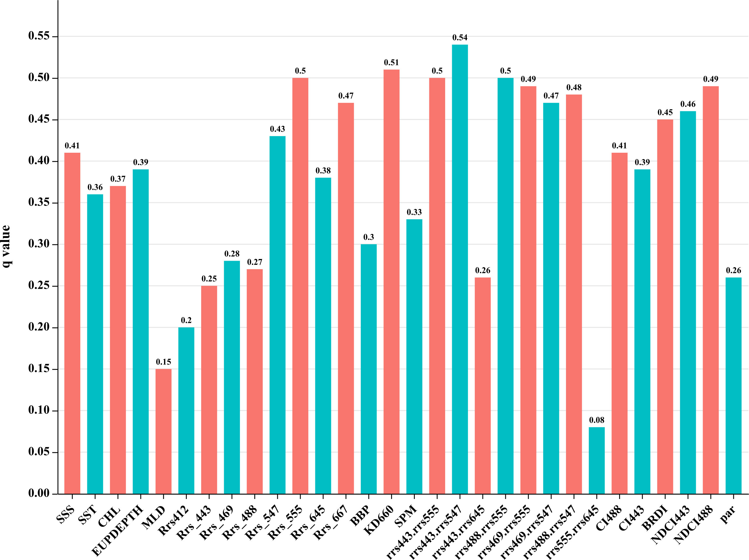
Figure 3 Geodetector factor detection results.

Figure 4

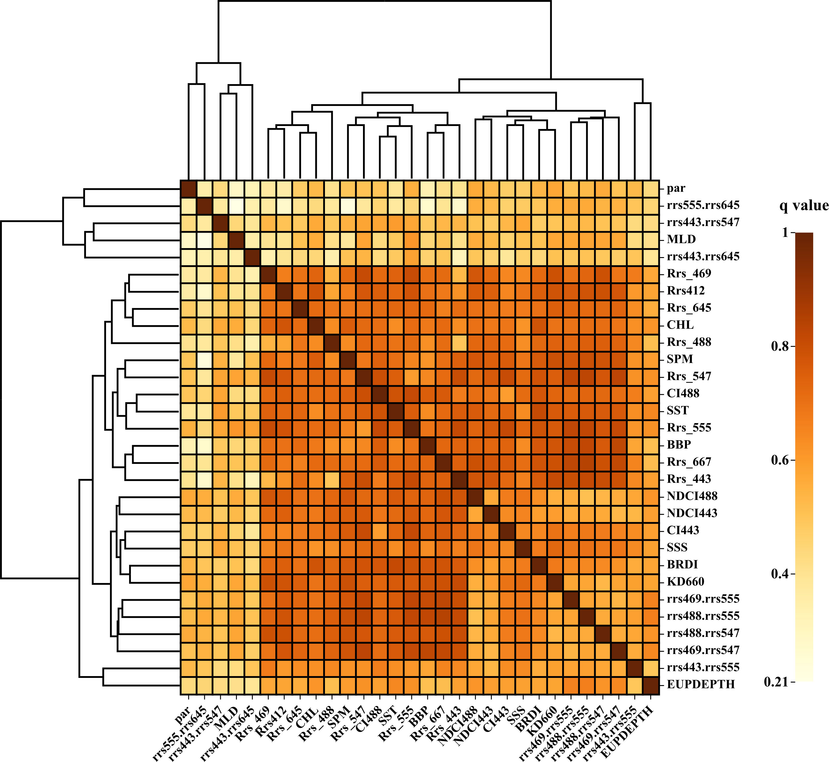
Figure 4 Heat map of geodetector interaction results.

3.2 Machine learning methods development and validation

3.2.1 Accuracy of the model on different datasets

The observed dataset was divided into training, validation, and test datasets. These datasets were used for the machine learning model training, hyperparameter tuning, and model performance validation. Hyperparameter tuning was performed using Bayesian optimization, as described by Shahriari and Swersky (Shahriari et al., 2016).

In this study, the six trained machine learning models were divided into two categories: BPNN, CNN, and ABNN, which are artificial neural networks (ANN), whereas AdaBoost, RF, and XGBoost are ensemble algorithms. These models can achieve high accuracy in multivariate regression tasks and exhibit good fitting performance for nonlinear functions. However, the large differences in data quantities for mineral, mixed, and organic water in the dataset are unfavorable for model training. They may lead to an increase in model variance. To enhance the generalization performance of the models, we applied a logarithmic transformation with a base of 10 to both the observed and estimated POC values. Table 2 shows the accuracy of the six machine learning models in estimating the log₁₀(POC) for the three datasets. Bold accuracy indicators represent the best performance for the corresponding dataset. Among the six models, the ensemble algorithms outperformed the neural network algorithms. The RF model achieved the best performance with an R² of 0.85, RMSE of 0.11 log₁₀(mg/m³), MAPE of 2.73%, variance of 0.09, and bias of 0.003 on the test dataset. This indicates that the RF model for estimating POC has good fitting and generalization capabilities.

Table 2

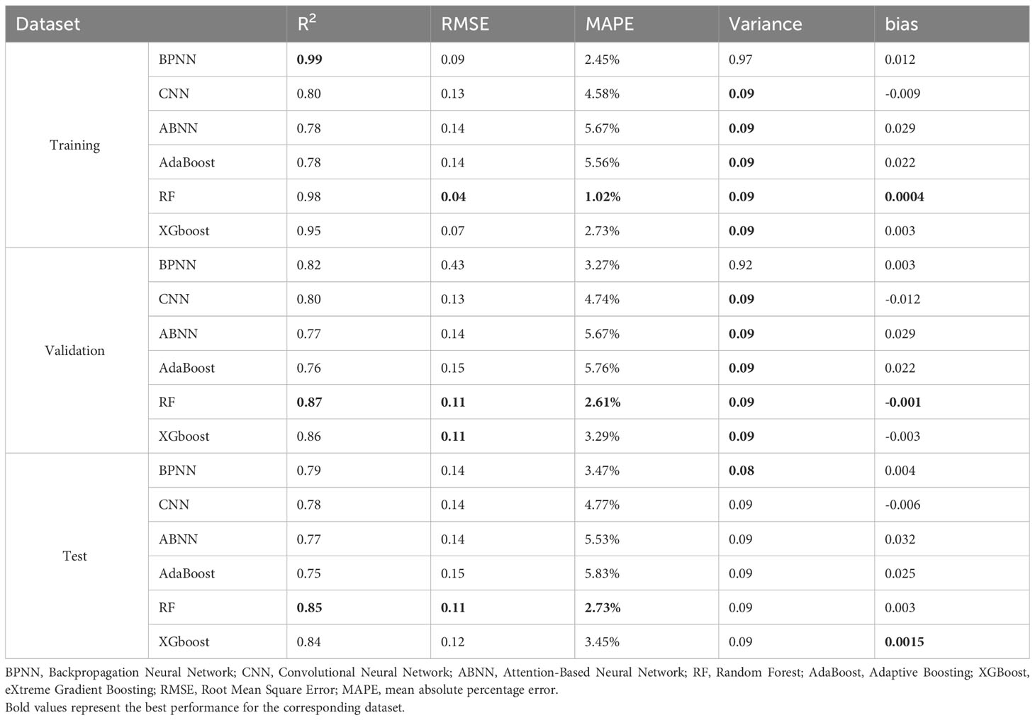
Table 2 Model accuracy on training, validation, and test datasets.

Normalized residuals were used to evaluate the fit of the statistical model and detect outliers. By observing the distribution of the normalized residuals, we can assess the model’s fit and identify outliers, which can help improve the model or clean the data. The normalized residuals of the predictions made by the six models on the test dataset was calculated. Figure 5 shows a scatterplot comparing the predicted and true values, where each point’s color represents the normalized residual’s magnitude. It can be visually observed that the BPNN performed the best among the neural network algorithms, with a MAPE of 3.471%. Among the ensemble algorithms, the RF performed the best. In contrast, the CNN, ABNN, and AdaBoost algorithms have a relatively poorer fit than the other models, and they have many data points with larger normalized residuals at high POC concentrations. This indicates that these three models have lower accuracy in estimating high POC concentrations. The BPNN, XGBoost, and RF algorithms exhibited a better fit, and RF performed well in predicting low and high POC concentrations. This is related to the strong noise immunity of RF, which can effectively reduce the effects of randomness and noise by means of multiple training and averaging predictions (Breiman, 2001), thus improving the robustness of the model and increasing the estimation accuracy of the POC.

Figure 5

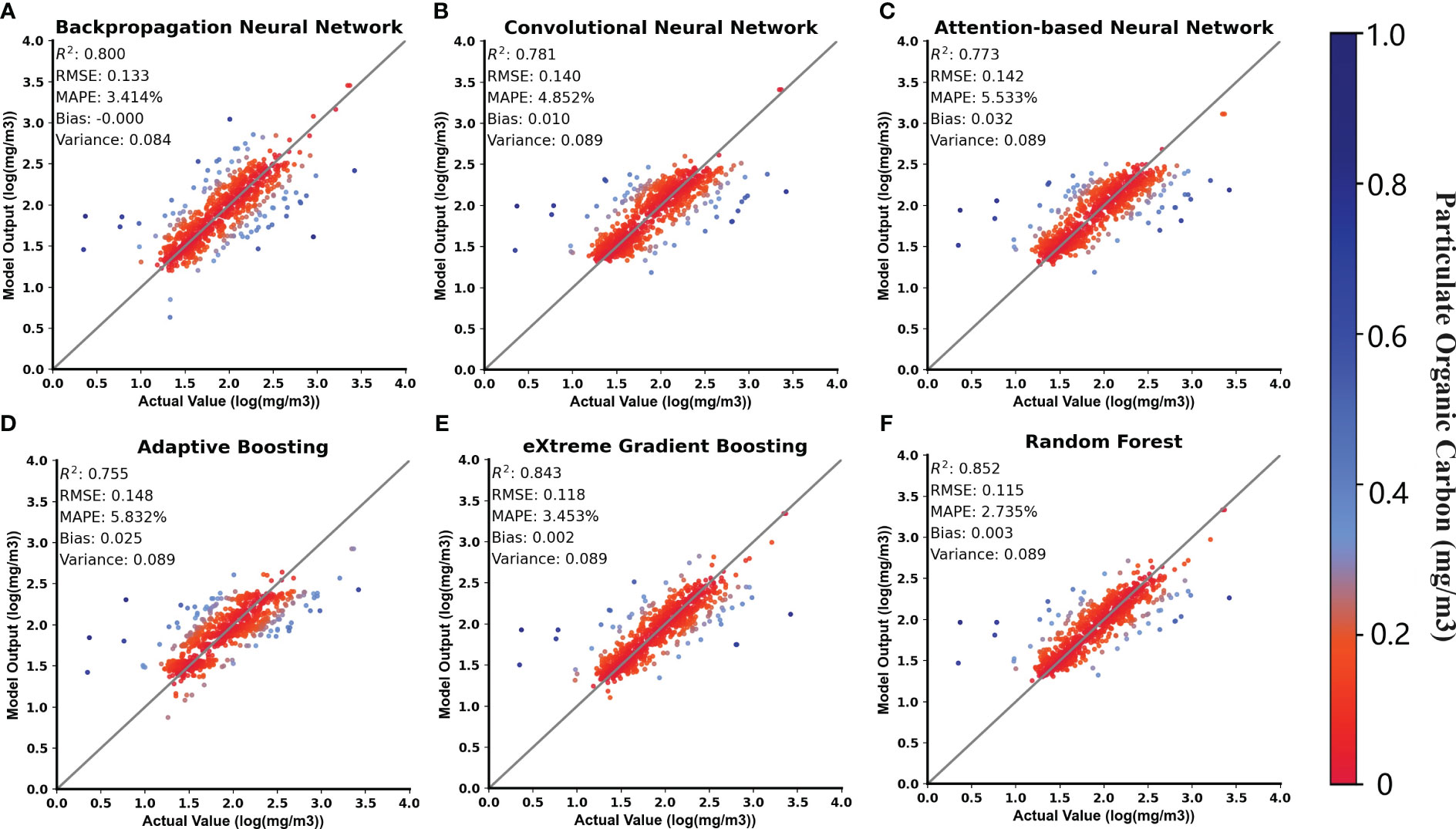
Figure 5 Scatterplot comparing model predicted and true values, where the color of the points represents the magnitude of the normalized residuals. (A–F) represent Backpropagation Neural Network, Convolutional Neural Network, Attention Neural Network, Adaptive Boosting, Extreme Gradient Boosting and Random Forest, respectively.

3.2.2 Accuracy of the model on different waters

To investigate the performance of the machine learning models in estimating POC for different water types, 200 matched POC data points belonging to mineral, organic, and mixed water were randomly sampled from the observed dataset. These data points were used to predict and assess the accuracy of the six trained machine-learning models. Table 3 presents the performance of the models in estimating log₁₀(POC) for the three water types. The bold indicators in the table represent the best performance of each machine learning model in estimating log₁₀(POC) for the three water types. It can be observed that all six machine learning models performed best in estimating the POC for mixed water. The RMSE is less than 0.1 log₁₀(mg/m³), the MAPE is less than 4%, the variance is less than 0.008, and the absolute value of the bias is less than 0.03. Figure 2 illustrates the significant differences in the POC concentration distributions in mineral, mixed, and organic water. These three water types represent low and high POC concentrations, respectively.

Table 3

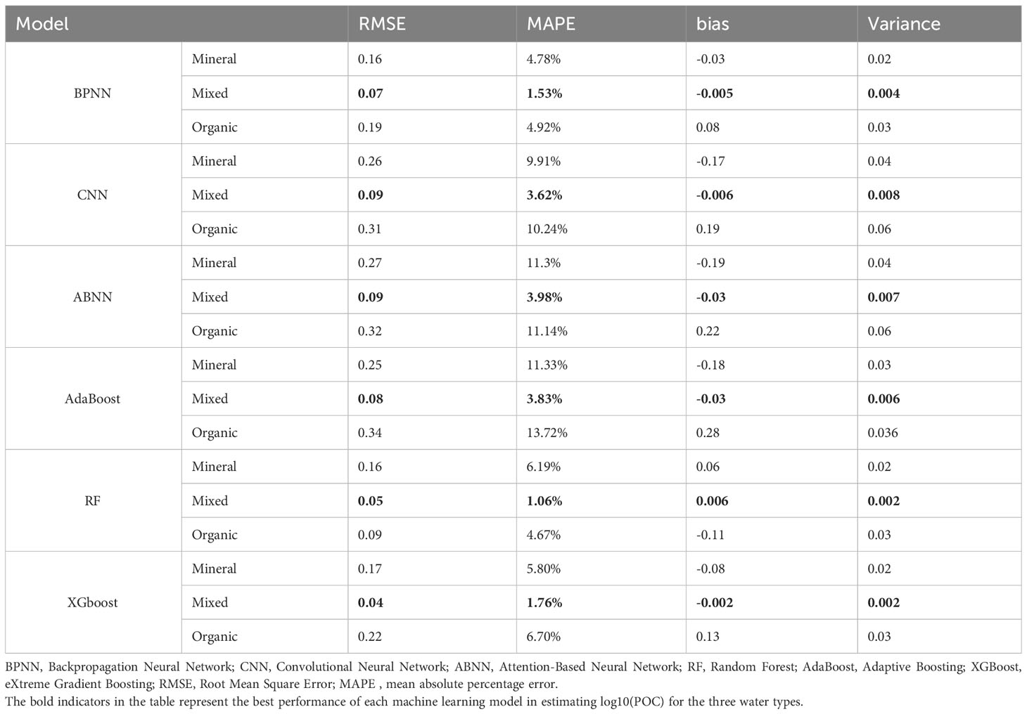
Table 3 Model performance for particulate organic carbon estimation in mineral, mixed, and organic water.

As shown in Table 3, except for the RF algorithm, the other five machine learning algorithms had higher prediction accuracies for mineral water than organic water, indicating that these five algorithms performed better in estimating low POC values. The RF algorithm had better estimation accuracy for organic water than mineral water, indicating that the RF model can better estimate high POC concentrations. Figure 6 normalizes the RMSE, MAPE, variance, and bias metrics, allowing for a visual comparison of the performance of each model for the three water types. The BPNN performed the best in mineral water, RF performed the best in mixed water, and RF demonstrated a significantly higher accuracy in estimating organic water than the other models. In contrast, CNN, ABNN, and AdaBoost performed relatively poorly for all three water types.

Figure 6

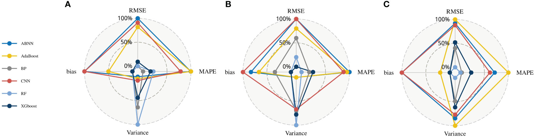
Figure 6 Radar plots of the performance of machine learning models for estimating particulate organic carbon in: (A) mineral water; (B) mixed water; (C) organic water.

In summary, the six machine learning models had good estimation performances for the moderate POC concentration range represented by mixed water (30 mg/m³–100 mg/m³). The BPNN achieved higher estimation accuracy for low POC concentrations represented by mineral water (10 mg/m³–30 mg/m³). In comparison, RF performed better in estimating high POC concentrations represented by organic water (>100 mg/m³).

3.3 Model application

3.3.1 Comparison with NASA’s POC products in space and time

This study compared global POC estimation products using RF and BPNN and band-ratio algorithms in terms of spatial and temporal analysis. The National Aeronautics and Space Administration (NASA) has utilized the blue-to-green band ratio algorithm to estimate POC concentrations in global oceans. This algorithm used the ratio of Rrs(443nm) to Rrs(555nm) from MODIS (Stramski et al., 2008). This study obtained NASA global POC products from the NASA OCEAN COLOR, spanning 2007 to 2017, for spatial and temporal analyses. Products from 2007 to 2016 were used for interannual POC variation analysis, whereas products from 2017 were used for spatial distribution analysis.

Figure 7 shows the spatial distribution of the global POC concentrations estimated using the RF, BPNN, and NASA standard POC product for 2017. Figure 7 shows that the spatial distributions of POC concentrations estimated by the three algorithms were similar worldwide. In global oceans, POC concentrations are mostly below 100 mg/m³ in the Atlantic, Pacific and Indian Oceans, but above 100 mg/m3 in the Arctic Ocean. Additionally, POC concentrations in coastal waters were significantly higher than in open ocean waters, because of the abundant land-based input of nutrients to coastal waters, and the intense water mass movements that cause bottom nutrients to be transported to the surface layer, which promotes phytoplankton growth and increases the efficiency of POC production (Lao et al., 2023b).

Figure 7

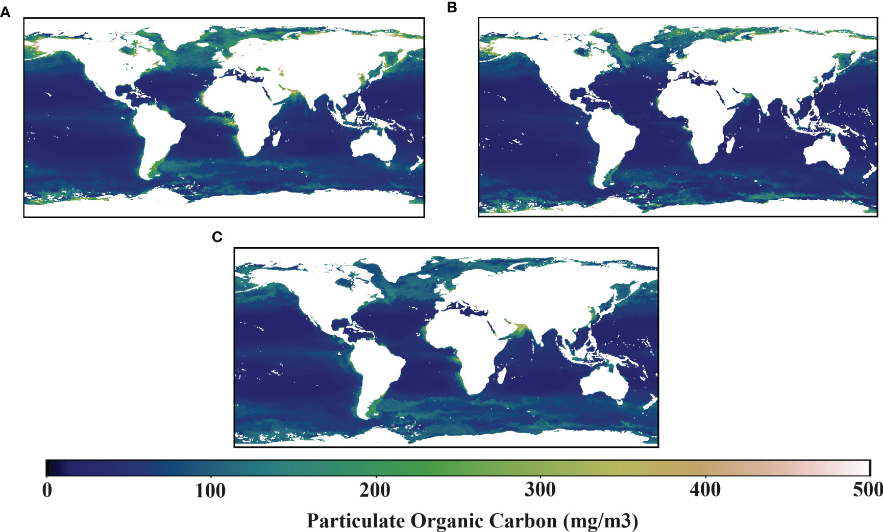
Figure 7 The global POC concentration distribution in 2017, estimated using three algorithms: (A) band ratio, (B) backpropagation neural network, and (C)random forest.

Figure 8 presents the deviation and percentage deviation of the global POC concentrations estimated by the RF and BPNN compared to NASA standard POC product. In the Arctic Ocean, the BPNN estimated significantly higher POC concentrations than the NASA standard POC product, with deviations exceeding 75 mg/m³ and percentage deviations exceeding 50%. However, the RF algorithm showed little deviation from the NASA standard POC product in the Arctic Ocean, with some regions showing lower POC concentrations of more than 50 mg/m³ and a percentage deviation exceeding 30%. In the Pacific, Atlantic, and Indian Oceans, the RF algorithm showed minimal deviation from the NASA standard POC product, with the Atlantic region having slightly lower POC concentrations and the Pacific and Indian Oceans having slightly higher POC concentrations. The deviation was less than 15 mg/m^3, and the percentage deviation was less than 40%. In contrast, the BPNN exhibited lower POC concentrations than the NASA standard POC product in the central Atlantic, central Pacific, and northern Indian Oceans. Although the deviation was within 25 mg/m³, the percentage deviation exceeded 50%, indicating that the BPNN can improve the estimation of POC concentrations in part of the open ocean. In the Antarctic Ocean, the RF algorithm and the BPNN estimated higher POC concentrations than the NASA standard POC product, with a deviation exceeding 50 mg/m³ and, in some regions, even exceeding 100 mg/m³, with a variance exceeding 50%. The NASA reference product uses the blue-green band ratio algorithm, which only considers Rrs and cannot effectively represent the influence of water components such as chlorophyll on POC. In polar ocean, the melting of glaciers increases the input of nutrient-rich water, promoting the growth of surface phytoplankton, leading to significantly higher chlorophyll-a concentrations compared to low-latitude seas (Babin et al., 2003; Arrigo, 2005; Steinacher et al., 2008). The RF and BPNN estimation models utilize Chl-a, which can effectively reflect the relationship between Chl-a and POC. Therefore, it is reasonable for RF and BPNN to exhibit certain differences from the NASA reference product in polar ocean. Moreover, in the Persian Gulf, Red Sea, and Arabian Sea, the RF algorithm showed significantly higher results than the reference products, with a deviation exceeding 100 mg/m³ and a percentage deviation exceeding 50%. These waters are strongly influenced by the monsoon winds of the Indian Ocean, which cause upwelling of deep water to the sea surface, promoting the mixing and transport of nutrients. Additionally, certain areas may also be affected by nutrient-rich water inputs from the Red Sea and the Persian Gulf, leading to possible occurrences of eutrophication in some sea areas (Kumar et al., 2000). The abundant nutrients facilitate the growth of phytoplankton in these waters, further promoting the production of POC and resulting in elevated POC concentrations.

Figure 8

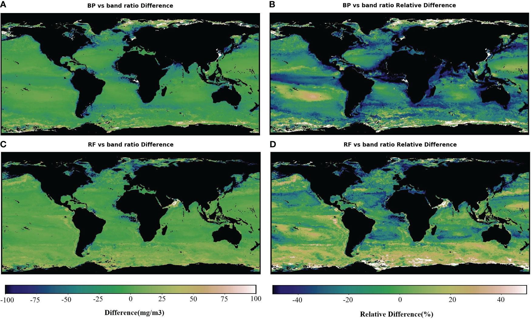
Figure 8 Deviation and percentage deviation between the 2017 global POC concentration estimated by random forest and backpropagation neural network algorithms and NASA’s particulate organic carbon standard algorithm. (A) Deviation of the back propagation neural network from the NASA standard algorithm for estimating POC. (B) Percentage deviation of the back propagation neural network from the NASA standard algorithm for estimating POC. (C) Deviation of the random forest from the NASA standard algorithm for estimating POC. (D) Percentage deviation of the random forest from the NASA standard algorithm for estimating POC.

Overall, the BPNN performed better than the RF algorithm in estimating open ocean POC concentrations. The RF algorithm showed a minor difference from the NASA standard POC product in the open ocean regions, with a percentage deviation of approximately 20%. However, in some coastal areas, the RF algorithm estimates higher POC concentrations than the NASA standard POC product, which helps improve the underestimation of POC concentrations by the band ratio algorithm in coastal waters.

Figure 9 shows the annual average variations in global POC concentrations estimated by the NASA standard POC product, the random forest (RF) algorithm, and the BPNN between 2007 and 2016. The annual average values estimated by the NASA standard POC product range from 85 mg/m³ to 100 mg/m³. In contrast, the annual average POC concentrations estimated using the BPNN and RF algorithm ranged from 60 mg/m³ to 70 mg/m³. The average percentage deviation of the BPNN from the NASA standard POC product is 27.15%. In comparison, the RF algorithm has an average deviation of 25.33% from the NASA standard POC product. This deviation can be attributed to two factors.

Figure 9

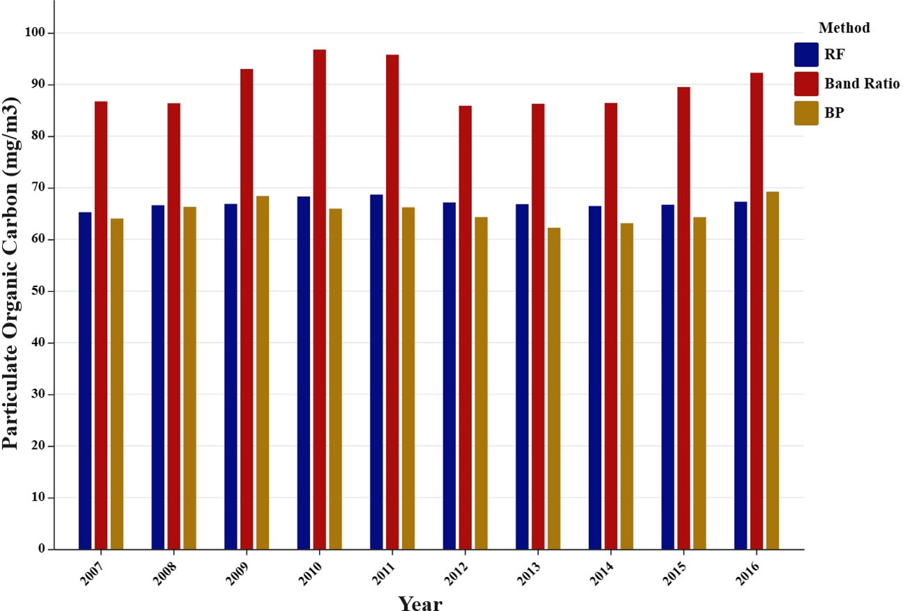
Figure 9 Annual changes in global POC from 2007 to 2016 as estimated by the blue-to-green band ratio, backpropagation neural network, and random forest algorithm.

First, the NASA global standard POC product includes estimates of POC concentrations in inland waters. Although inland waters have smaller surface areas than oceans, they may have higher POC contents. This is because inland waters are usually shallower, making it easier for light to penetrate to the bottom of the water. This promotes active photosynthesis and higher biological productivity. At the same time, inland waters are influenced by input substances, organisms, and human activities from land, such as organic matter, nutrients, and pollutants carried by rivers, which may result in relatively higher POC content (Yang et al., 2016). This affected the average value of the NASA global POC product to some extent. Second, POC concentrations can exceed 10,000 mg/m3 (Steinacher et al., 2008). The measured POC values collected in this study range from 1.46 mg/m3 to 4743 mg/m3, and there are relatively few measured points with high POC concentrations. This caused the trained model to underestimate the values of high POC concentrations. Combining these two factors, the machine learning model estimates global average annual POC value is lower than the average annual POC value in NASA’s standard POC product.

Figure 9 shows that, from 2007 to 2011, the global mean POC estimated by the RF algorithm and the NASA standard product increased. From 2011 to 2014, there was a slight decrease in global mean POC; from 2014 to 2016, there was a subsequent increase. In contrast, the BPNN estimated an increase in global POC from 2007 to 2009, a decrease from 2009 to 2013, and an increase from 2013 to 2017. Regarding the annual trends, the RF estimation of the global mean POC showed better consistency with the NASA standard product than with the BPNN, and the RF-estimated POC product can be used to investigate the spatial and temporal trends in POC in various global ocean areas.

3.3.2 Results of the random forest algorithm for estimating global surface POC

The BPNN and random forest algorithm performed well in estimating global surface POC concentrations. However, the Random Forest algorithm provides a better estimate of POC in coastal waters. This study estimated the global surface POC concentration from 2007 to 2016 using the random forest algorithm and discussed the variations in POC in different ocean regions during this period.

Figure 10 illustrates the distribution of global surface POC concentrations from 2007 to 2016, which indicates a consistent spatial distribution of POC over the 10-year period. The global biomass of zooplankton is higher in the coastal zone than in the open ocean due to sufficient land inputs, abundant sunlight and nutrient-rich currents. The distribution of surface POC is higher in the coastal zone than in the open ocean. Figure 10 shows that surface POC concentrations are significantly higher in nearshore areas (e.g., the Arabian Sea, off China and off Angola) than in other areas. Indeed, the distribution of surface POC concentrations is also related to latitude. Figure 10 shows that high-latitude regions, such as the Arctic Ocean, Antarctic waters, North and South Atlantic, and North and South Pacific, have higher surface POC concentrations than middle and low-latitude regions. This was related to several factors.

Figure 10

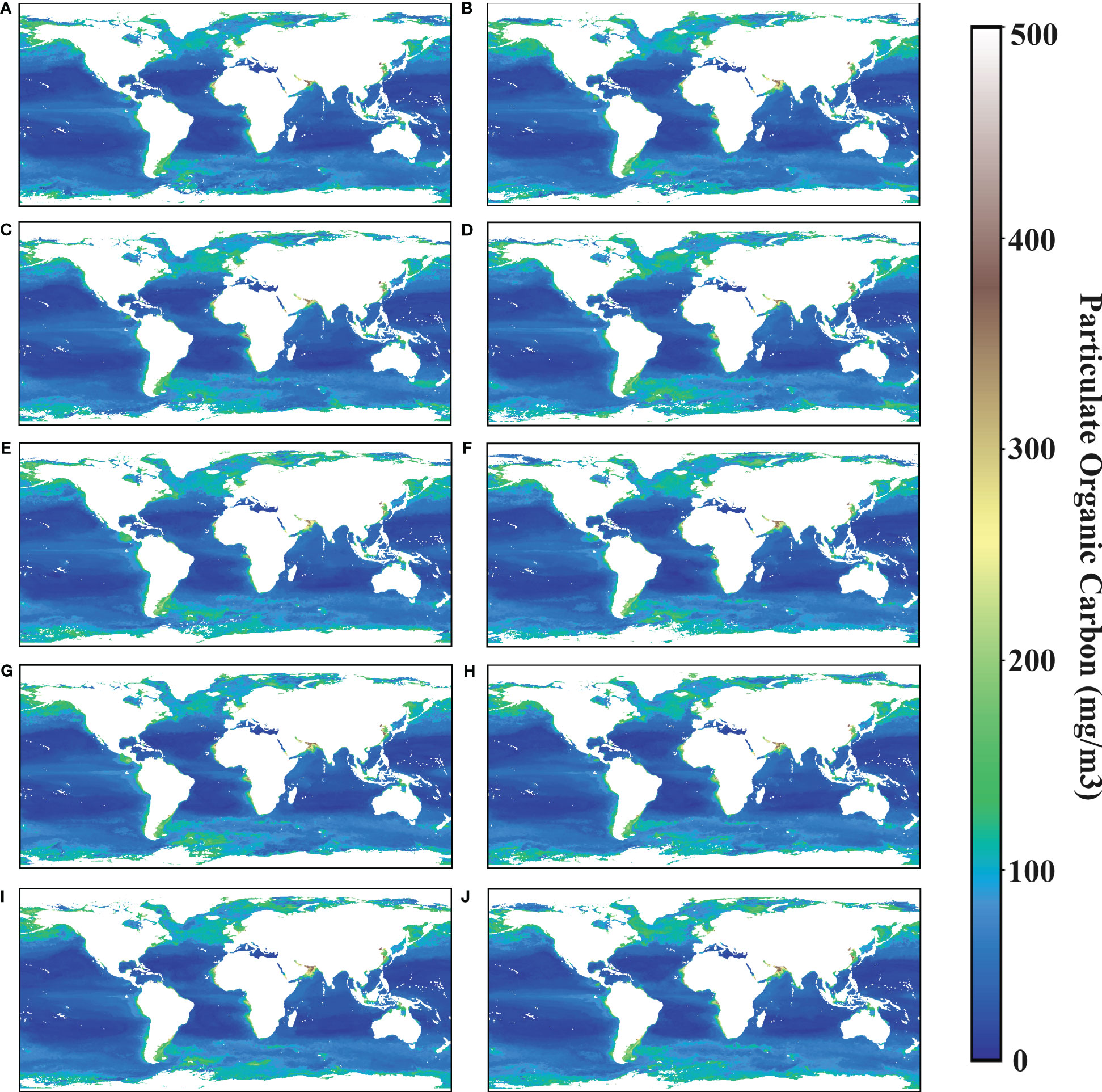
Figure 10 (A–J) Represent global particulate organic carbon distribution from 2007 to 2016 estimated using the random forest algorithm.

First, nutrients provided by water transport have a significant impact on the growth of phytoplankton (Sardessai et al., 2010; Xu et al., 2019; Lao et al., 2023b), including enhanced vertical mixing (Lao et al., 2023c), which directly affects the distribution of organic matter content in the ocean (Yamashita et al., 2019; Wang et al., 2021).

Water masses are more strongly mixed at high latitudes due to cold water, glacial melt, polar eddies, and boundary currents, and these fluid movements bring deep organic matter (e.g., dead organisms and detritus) to the surface of the oceans, which increases the organic content of the surface layer, enhances the productivity of marine organisms, and increases the production of POC. Secondly, high latitudes have relatively weak sunlight, especially in winter. This limits the photosynthesis of phytoplankton. As a result, they focus on growth and reproduction during the shorter summer months, leading to higher surface POC concentrations (Babin et al., 2003; Arrigo, 2005; Steinacher et al., 2008).

Figure 11 shows the results of classifying the POC products estimated using RF into mineral water, mixed water and organic water for the period 2007-2016. Mineral water is mainly found in the Arctic Ocean, Antarctic waters, and regions between 20° and 40° north and south latitudes. Mixed water is predominantly found in equatorial regions and the North and South Atlantic and Pacific waters. Organic water was distributed along the continental margins. Although the POC concentration is higher in the Arctic Ocean, intense ocean currents and glacial melting in polar regions result in higher concentrations of suspended particles. This classification implies that the Arctic Ocean region falls under the mineral water category.

Figure 11

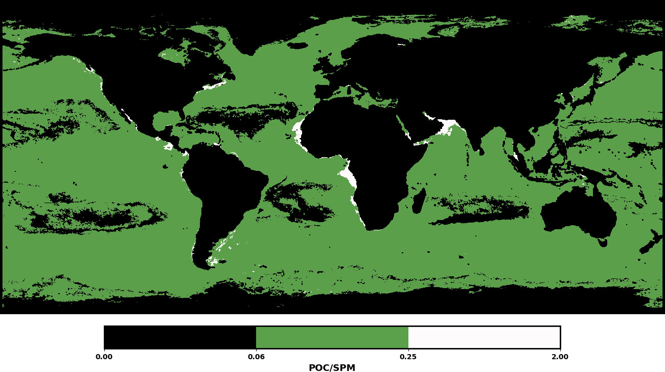
Figure 11 Distribution of mineral, mixed, and organic water according to particulate organic carbon/suspended particulate matter.

Fifty sampling points were selected from the three waters mentioned above. POC concentrations at the sampling points collected between 2007 and 2016 were extracted. The average value of these 50 concentrations represented the average POC concentration of the corresponding waters in the current year. A line graph was plotted to examine the variations in POC concentrations over time in different waters. Figure 12 shows that the POC concentrations in the mineral and mixed water remained relatively stable over the 10-year period. However, the POC concentration in organic water decreased from 2009 to 2010, increased from 2010 to 2012, and decreased again from 2015 to 2016. POC concentrations at the sea surface may be related to the El Niño phenomenon. El Niño leads to an increase in the sea surface temperature in the equatorial Pacific. The stratification of the water column become more pronounced with the increase in sea surface temperature, inhibiting the upwelling of deep eutrophic water to the upper layers, thus affecting phytoplankton growth, which further led to a decrease in primary productivity and a decrease in the concentration of POC in the surface layer of the ocean. Additionally, El Niño can cause changes in wind patterns and ocean circulation, which may alter the distribution of nutrients in the ocean and affect phytoplankton (Chavez et al., 1999; Behrenfeld et al., 2006; Dore et al., 2009; Lao et al., 2023b). Indeed, El Niño events in both 2009-2010 and 2015-2016 can partially explain the variations in POC concentrations observed in organic waters, as shown in Figure 12.

Figure 12

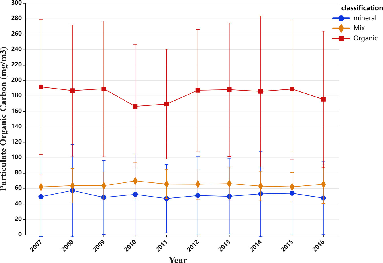
Figure 12 Changes in annual mean values of mineral, mixed, and organic water sampling sites from 2007 to 2016.

3.4 Limitations

This study compared the performances of six machine learning algorithms in estimating POC on the ocean surface. The RF algorithm improved the estimation of POC in areas with complex optical conditions near the coast. A brief discussion was also conducted on the spatiotemporal distribution of the global POC based on RF. However, this study still has some limitations that need to be addressed. These limitations are listed below:

1) The data collected were unevenly distributed in terms of spatial coverage. Most data points are concentrated in the Atlantic, Pacific, and Mediterranean Seas. There is a lack of sufficient measured data in the Indian Ocean and the Arctic Ocean, as well as in some eutrophic regions, such as the Red Sea, Arabian Sea, and Persian Gulf. This can affect the accuracy of the machine-learning model and result in an underestimation of POC concentrations in areas with complex optical conditions near the coast. In the future, more POC data should be collected on a global scale, and the accuracy of the data should be controlled to improve the model’s accuracy.

2) This study only produced annual POC products from 2007 to 2016. However, the POC exhibited strong seasonal variability. Therefore, conducting monthly POC estimation in the future would be beneficial, allowing for a more accurate investigation of the spatiotemporal characteristics of global POC.

4 Conclusions

This article is based on a large amount of open-source data and has created a large in-situ POC dataset distributed in various oceans around the world. By using geodetector, twenty factors closely related to oceanic POC concentration were screened. The dataset was partitioned based on the POC/SPM to ensure the training, validation, and test datasets had similar data distributions. Six machine learning methods were used to construct POC estimation models, with the accuracy being evaluated. By comparing the performances of six different machine learning models and their performances in different water types, it was found that the random forest algorithm achieved the highest accuracy on the test dataset. The RMSE was measured at 0.11 log10(g/m3), the MAPE was 2.73%, the variance reached 0.09, and the bias was only 0.003. The RF estimation of POC had the highest accuracy in organic waters, and the BPNN had the highest accuracy in mineral waters. Furthermore, the RF estimation results showed better consistency with NASA standard products, thereby enhancing the accuracy of POC estimation in optically complex seas. In future research, a high-precision POC estimation model should be constructed based on a large amount of measured data in all types of waters.

Based on the RF model, POC products from 2007 to 2017 were generated, and the spatio-temporal distribution characteristics of global POC during this 10-year period were investigated. The results indicated that the POC concentration in high-latitude seas was higher than that in mid-latitude and low-latitude seas. This could be attributed to the strong fluid motions in high-latitude regions, such as polar eddies and boundary currents, which intensify the mixing of water masses and bring organic materials from deeper layers to the ocean surface, thereby promoting the growth of phytoplankton and increasing the concentration of surface POC. Additionally, the El Niño phenomenon may be associated with interannual variations in POC, as higher sea surface temperatures and increased seawater stratification during the El Niño period reduce the upwelling of nutrients from the seafloor, restricting phytoplankton growth and thus lowering the concentration of POC in the surface layer. El Niño events in both 2009-2010 and 2015-2016 can partially explain the variations in POC concentrations observed in organic waters. In future studies, seasonal-scale variations in POC should be investigated, and the relevant drivers of changes in POC concentrations should be studied in greater depth.

Data availability statement

The original contributions presented in the study are included in the article/Supplementary Material. Further inquiries can be directed to the corresponding author.

Author contributions

HW: Conceptualization, Funding acquisition, Methodology, Project administration, Supervision, Writing – review & editing. LC: Data curation, Formal Analysis, Methodology, Resources, Software, Validation, Visualization, Writing – original draft, Writing – review & editing. LW: Resources, Software, Validation, Visualization, Writing – review & editing. RS: Investigation, Writing – review & editing. ZZ: Data curation, Writing – review & editing.

Funding

The author(s) declare financial support was received for the research, authorship, and/or publication of this article. This research was funded by Key Laboratory of Land Satellite Remote Sensing Application, Ministry of Natural Resources of the People’ s Republic of China, grant numbers G202211, and the Ministry of Education Industry- University Collaborative Education Project, grant numbers 220504039151258, and the Fundamental Research Funds for the Central Universities, grant numbers 18CX02064A.

Acknowledgments

We are grateful to the NASA Ocean Biology Processing Group for providing MODIS products (https://oceancolor.gsfc.nasa.gov/) and in situ data from seabass (https://seabass.gsfc.nasa.gov/); We are grateful to Copernicus Marine Service (https://marine.copernicus.eu/) providing remote sensing reanalysis data.

Conflict of interest

The authors declare that the research was conducted in the absence of any commercial or financial relationships that could be construed as a potential conflict of interest.

Publisher’s note

All claims expressed in this article are solely those of the authors and do not necessarily represent those of their affiliated organizations, or those of the publisher, the editors and the reviewers. Any product that may be evaluated in this article, or claim that may be made by its manufacturer, is not guaranteed or endorsed by the publisher.

Supplementary material

The Supplementary Material for this article can be found online at: https://www.frontiersin.org/articles/10.3389/fmars.2023.1295874/full#supplementary-material

References

Arrigo K. R. (2005). Marine microorganisms and global nutrient cycles. nat. 437, 349. doi: 10.1038/nature04265

CrossRef Full Text | Google Scholar

Babin M., Morel A., Fournier-Sicre V., Fell F., Stramski D. (2003). Light scattering properties of marine particles in coastal and open ocean waters as related to the particle mass concentration. Limnology Oceanogr. 48 (2), 843–859. doi: 10.4319/lo.2003.48.2.0843

CrossRef Full Text | Google Scholar

Behrenfeld M. J., O Malley R. T., Siegel D. A., Mcclain C. R., Sarmiento J. L., Feldman G. C., et al. (2006). Climate-driven trends in contemporary ocean productivity. Nature 444 (7120), 752–755. doi: 10.1038/nature05317

PubMed Abstract | CrossRef Full Text | Google Scholar

Bonelli A. G., Loisel H., Jorge D. S. F., Mangin A., D'Andon O. F., Vantrepotte V. (2022). A new method to estimate the dissolved organic carbon concentration from remote sensing in the global open ocean. Remote Sens. Environ. 281, 113227. doi: 10.1016/j.rse.2022.113227

CrossRef Full Text | Google Scholar

Bopp L., Le Quéré C., Heimann M., Manning A. C., Monfray P. (2002). Climate-induced oceanic oxygen fluxes: Implications for the contemporary carbon budget. Global Biogeochem. Cycles. 16 (2), 6–1-6-13. doi: 10.1029/2001GB001445

CrossRef Full Text | Google Scholar

Breiman L. (2001). Random forests. Mach. Learn. 45 (1), 5–32. doi: 10.1023/A:1010933404324

CrossRef Full Text | Google Scholar

Brewin R. J. W., Sathyendranath S., Platt T., Bouman H., Ciavatta S., Dall'Olmo G., et al. (2021). Sensing the ocean biological carbon pump from space: A review of capabilities, concepts, research gaps and future developments. Earth-Sci. Rev. 217, 103604. doi: 10.1016/j.earscirev.2021.103604

CrossRef Full Text | Google Scholar

Cai S., Wu M., Le C. (2022). Satellite observation of the long-term dynamics of particulate organic carbon in the east China Sea based on a hybrid algorithm. Remote Sens. 14 (13), 3220. doi: 10.3390/rs14133220

CrossRef Full Text | Google Scholar

Cao F., Ge Y., Wang J. (2013). Optimal discretization for geographical detectors-based risk assessment. GIScience Remote Sensing. 50 (1), 78–92. doi: 10.1080/15481603.2013.778562

CrossRef Full Text | Google Scholar

Chavez F. P., Strutton P. G., Friederich G. E., Feely R. A., Feldman G. C., Foley D. G., et al. (1999). Biological and chemical response of the equatorial pacific ocean to the 1997-98 El Niño. Science 286 (5447), 2126–2131. doi: 10.1126/science.286.5447.2126

PubMed Abstract | CrossRef Full Text | Google Scholar

Devi G. K., Ganasri B. P., Dwarakish G. S. (2015). Applications of remote sensing in satellite oceanography: A review. Aquat. Procedia. 4, 579–584. doi: 10.1016/j.aqpro.2015.02.075

CrossRef Full Text | Google Scholar

Dore J. E., Lukas R., Sadler D. W., Church M. J., Karl D. M. (2009). Physical and biogeochemical modulation of ocean acidification in the central North Pacific. Proc. Natl. Acad. Sci. 106 (30), 12235–12240. doi: 10.1073/pnas.0906044106

CrossRef Full Text | Google Scholar

Doney S. C., Fabry V. J., Feely R. A., Kleypas J. A. (2009). Ocean acidification: the other CO₂ problem. Annu. Rev. Mar. Sci. 1(1), 169–192. doi: 10.1146/annurev.marine.010908.163834

CrossRef Full Text | Google Scholar

Elhorst J. P. (2010). Spatial Panel Data Models. In: Fischer M.M., Getis A. (eds). Handbook of Applied Spatial Analysis: Software Tools, Methods and Applications (Berlin, Heidelberg: Springer Berlin Heidelberg). 377–407. doi: 10.1007/978-3-642-03647-7_19

CrossRef Full Text | Google Scholar

Freund Y., Schapire R. E. (1995). "A decision-thoretic generalization of on-line learning and an application to boosting," in Computational Learning Theory. EuroCOLT 1995. Lecture Notes in Computer Science, eds Vitányi P. (Berlin, Heidelberg: Springer) 55 (1), 119–139. doi: 10.1007/3-540-59119-2_166

CrossRef Full Text | Google Scholar

Gardner W. D., Mishonov A. V., Richardson M. J. (2006). Global POC concentrations from in-situ and satellite data. Deep Sea Res. Part II: Topical Stud. Oceanogr. 53 (5), 718–740. doi: 10.1016/j.dsr2.2006.01.029

CrossRef Full Text | Google Scholar

Good S., Fiedler E., Mao C., Martin M. J., Worsfold M. (2020). The current configuration of the OSTIA system for operational production of foundation sea surface temperature and ice concentration analyses. Remote Sens. 12 (4), 720–. doi: 10.3390/rs12040720

CrossRef Full Text | Google Scholar

Hayley E. K., Victor M. V., Brewin R. J. W., Giorgio D., Hickman A. E., Thomas J., et al. (2017). Validation and intercomparison of ocean color algorithms for estimating particulate organic carbon in the oceans. Front. Mar. Sci. 4. doi: 10.3389/fmars.2017.00251

CrossRef Full Text | Google Scholar

Jahnke, Richard A. (1996). The global ocean flux of particulate organic carbon: Areal distribution and magnitude. Global Biogeochem. Cycles. 10 (1), 71–88. doi: 10.1029/95GB03525

CrossRef Full Text | Google Scholar

Jiang G., Loiselle S. A., Cai W., Yang J., Duan (2015). Remote sensing of particulate organic carbon dynamics in a eutrophic lake (Taihu Lake, China). Sci. Total Environ. 532, 245–254. doi: 10.1016/j.scitotenv.2015.05.120

PubMed Abstract | CrossRef Full Text | Google Scholar

Kim M., Hwang J., Kim G., Na T., Kim T., Hyun J. (2022). Carbon cycling in the East Sea (Japan Sea): A review. Front. Mar. Sci. 9. doi: 10.3389/fmars.2022.938935

PubMed Abstract | CrossRef Full Text | Google Scholar

Krishnapuram B., Shah M., Smola A., Aggarwal C., Shen D., Rastogi R. (2016). KDD '16: The 22nd ACM SIGKDD International Conference on Knowledge Discovery and Data Mining (San Francisco, California, USA: Association for Computing Machinery). doi: 10.1145/2939672

CrossRef Full Text | Google Scholar

Kumar S. P., Madhupratap M., Kumar M. D., Gauns M., Muraleedharan P. M., Sarma V. V. S. S., et al. (2000). Physical control of primary productivity on a seasonal scale in central and eastern Arabian Sea. J. Earth Syst. Sci. 109, 433–441. doi: 10.1007/BF02708331

CrossRef Full Text | Google Scholar

Lao Q., Chen F., Jin G., Lu X., Chen C., Zhou X., et al. (2023a). Characteristics and mechanisms of typhoon-induced decomposition of organic matter and its implication for climate change. J. Geophysical Research: Biogeosciences 128 (6), e2023JG007518. doi: 10.1029/2023JG007518

CrossRef Full Text | Google Scholar

Lao Q., Liu S., Ling Z., Jin G., Chen F., Chen C., et al. (2023b). External dynamic mechanisms controlling the periodic offshore blooms in Beibu gulf. J. Geophysical Research: Oceans 128 (6), e2023JC019689. doi: 10.1029/2023JC019689

CrossRef Full Text | Google Scholar

Lao Q., Lu X., Chen F., Jin G., Chen C., Zhou X., et al. (2023c). Effects of upwelling and runoff on water mass mixing and nutrient supply induced by typhoons: Insight from dual water isotopes tracing. Limnology Oceanogr. 68 (1), 284–295. doi: 10.1002/lno.12266

CrossRef Full Text | Google Scholar

Lavergne T., Srensen A. M., Kern S., Tonboe R., Pedersen L. T. (2019). Version 2 of the EUMETSAT OSI SAF and ESA CCI sea-ice concentration climate data records. Cryosphere. 13 (1), 49–78. doi: 10.5194/tc-13-49-2019

CrossRef Full Text | Google Scholar

Le C., Lehrter J. C., Hu C., Macintyre H., Beck M. W. (2017). Satellite observation of particulate organic carbon dynamics on the Louisiana continental shelf. J. Geophysical Research: Oceans. 122 (1), 555–569. doi: 10.1002/2016JC012275

CrossRef Full Text | Google Scholar

Lecun Y., Bengio Y., Hinton G. (2015). Deep learning. Nature 521 (7553), 436–444. doi: 10.1038/nature14539

PubMed Abstract | CrossRef Full Text | Google Scholar

Lecun Y., Bottou L., Bengio Y., Haffner P. (1998). Gradient-based learning applied to document recognition. Proc. IEEE. 86 (11), 2278–2324. doi: 10.1109/5.726791

CrossRef Full Text | Google Scholar

Liu H., Li Q., Bai Y., Yang C., Wang J., Zhou Q., et al. (2021). Improving satellite retrieval of oceanic particulate organic carbon concentrations using machine learning methods. Remote Sens. Environ. 256, 112316. doi: 10.1016/j.rse.2021.112316

CrossRef Full Text | Google Scholar

Loisel H., Bosc E., Stramski D., Oubelkheir K., Deschamps P. Y. (2001). Seasonal variability of the backscattering coefficient in the Mediterranean Sea based on satellite SeaWiFS imagery. Geophys. Res. Lett. 28 (22), 4203–4206. doi: 10.1029/2001GL013863

CrossRef Full Text | Google Scholar

Loisel H., Nicolas J., Deschamps P., Frouin R. (2002). Seasonal and inter-annual variability of particulate organic matter in the global ocean. Geophys. Res. Lett. 29 (24), 49. doi: 10.1029/2002GL015948

CrossRef Full Text | Google Scholar

Maritorena S., D'Andon O. H. F., Mangin A., Siegel D. A. (2010). Merged satellite ocean color data products using a bio-optical model: Characteristics, benefits and issues. Remote Sens. Environ. 114 (8), 1791–1804. doi: 10.1016/j.rse.2010.04.002

CrossRef Full Text | Google Scholar

Martiny A. C., Vrugt J. A., Lomas M. W. (2014). Concentrations and ratios of particulate organic carbon, nitrogen, and phosphorus in the global ocean. Sci. Data. 1 (1), 140048. doi: 10.1038/sdata.2014.48

PubMed Abstract | CrossRef Full Text | Google Scholar

Massari C., Camici S., Ciabatta L., Brocca L. (2018). Exploiting satellite-based surface soil moisture for flood forecasting in the Mediterranean area: state update versus rainfall correction. Remote Sensing. 10 (2), 292. doi: 10.3390/rs10020292

CrossRef Full Text | Google Scholar

Mcculloch W. S., Pitts W. (1990). A logical calculus of the ideas immanent in nervous activity. Bull. Math. Biol. 52 (1), 99–115. doi: 10.1007/BF02459570

PubMed Abstract | CrossRef Full Text | Google Scholar

Merchant C. J., Embury O., Bulgin C. E., Block T., Donlon C. (2019). Satellite-based time-series of sea-surface temperature since 1981 for climate applications. Sci. Data. 6 (1), 223. doi: 10.1038/s41597-019-0236-x

PubMed Abstract | CrossRef Full Text | Google Scholar

Morel A., Prieur L. (1977). Analysis of variations in ocean color. Limnol. Oceanogr. 22 (4), 709–722. doi: 10.4319/lo.1977.22.4.0709

CrossRef Full Text | Google Scholar

O'Reilly J. E. (2000). Ocean color chlorophyll algorithms for SeaWiFS, OC2, and OC4 : Ver 4. SeaWiFS Postlaunch Calibration and Validation Analyses, Part 3. NASA Tech. Memo. 11, 9–27. Available at: https://cir.nii.ac.jp/crid/1570572701233940096.

Google Scholar

O'Reilly J. E., Werdell P. J. (2019). Chlorophyll algorithms for ocean color sensors-OC4, OC5 & OC6. Remote Sens. Environ.: Interdiscip. J. 229, 32–47. doi: 10.1016/j.rse.2019.04.021

CrossRef Full Text | Google Scholar

Sardessai S., Shetye S., Maya M. V., Mangala K. R., Prasanna Kumar S. (2010). Nutrient characteristics of the water masses and their seasonal variability in the eastern equatorial Indian Ocean. Mar. Environ. Res. 70 (3), 272–282. doi: 10.1016/j.marenvres.2010.05.009

PubMed Abstract | CrossRef Full Text | Google Scholar

Sarmiento J. L. (2006). Ocean Biogeochemical Dynamics. Princeton University Press. doi: 10.1515/9781400849079

CrossRef Full Text | Google Scholar

Sauzède R., Claustre H., Uitz J., Jamet C., Dall'Olmo G., D'Ortenzio F., et al. (2016). A neural network-based method for merging ocean color and Argo data to extend surface bio-optical properties to depth: Retrieval of the particulate backscattering coefficient. J. Geophysical Research: Oceans. 121 (4), 2552–2571. doi: 10.1002/2015JC011408

CrossRef Full Text | Google Scholar

Sauzède R., Johnson J. E., Claustre H., Camps-Valls G., Ruescas A. B. (2020). ESTIMATION OF OCEANIC PARTICULATE ORGANIC CARBON WITH MACHINE LEARNING. ISPRS Ann. Photogramm. Remote Sens. Spatial Inf. Sci. 2, 949–956. doi: 10.5194/isprs-annals-V-2-2020-949-2020

CrossRef Full Text | Google Scholar

Sauzède R., Claustre H., R., Remanan P., Uitz J., Guinehut S., et al. (2021). New global vertical distribution of gridded particulate organic carbon and chlorophyll-a concentration using machine learning for cmems. 9th EuroGOOS International conference. Shom and Ifremer and EuroGOOS AISBL. (Brest, France), 313–320. https://hal.science/hal-03335370v2.

Google Scholar

Sawaya K. E., Olmanson L. G., Heinert N. J., Brezonik P. L., Bauer M. E. (2003). Extending satellite remote sensing to local scales: land and water resource monitoring using high-resolution imagery. Remote Sens. Environ. 88 (1), 144–156. doi: 10.1016/j.rse.2003.04.006

CrossRef Full Text | Google Scholar

Shahriari B., Swersky K., Wang Z., Adams R. P., De Freitas N. (2016). Taking the human out of the loop: A review of Bayesian optimization. Proc. IEEE. 104 (1), 148–175. doi: 10.1109/JPROC.2015.2494218

CrossRef Full Text | Google Scholar

Shi Y., Zhang D., Ji H., Dai R. (2019). Application of synchrosqueezed wavelet transform in microseismic monitoring of mines. IOP Conference Series: Earth and Environmental Science 384 (01), 012075. doi: 10.1088/1755-1315/384/1/012075

CrossRef Full Text | Google Scholar

Son Y. B., Gardner W. D., Mishonov A. V., Richardson M. J. (2009). Multispectral remote-sensing algorithms for particulate organic carbon (POC): The Gulf of Mexico. Remote Sens. Environ. 113 (1), 50–61. doi: 10.1016/j.rse.2008.08.011

CrossRef Full Text | Google Scholar

Song Y., Wang J., Ge Y., Xu C. (2020). An optimal parameters-based geographical detector model enhances geographic characteristics of explanatory variables for spatial heterogeneity analysis: cases with different types of spatial data. GISci. Remote Sens. 57 (5), 593–610. doi: 10.1080/15481603.2020.1760434

CrossRef Full Text | Google Scholar

Steinacher M., Joos F., Frölicher T. L., P. G. K., Doney S. C. (2008). Imminent ocean acidification projected with the NCAR global coupled carbon cycle-climate model. Biogeosciences Discussions 5 (4), 4353–4393. doi: 10.5194/bgd-5-4353-2008

CrossRef Full Text | Google Scholar

Stramski D., Joshi I., Reynolds R. A. (2022). Ocean color algorithms to estimate the concentration of particulate organic carbon in surface waters of the global ocean in support of a long-term data record from multiple satellite missions. Remote Sens. Environ. 269, 112776. doi: 10.1016/j.rse.2021.112776

CrossRef Full Text | Google Scholar

Stramski D., Reynolds R. A., Babin M., Kaczmarek S., Lewis M. R., Röttgers R., et al. (2008). Relationships between the surface concentration of particulate organic carbon and optical properties in the eastern South Pacific and eastern Atlantic Oceans. Biogeosciences 5 (1), 171–201. doi: 10.5194/bg-5-171-2008

CrossRef Full Text | Google Scholar

Stramski D., Reynolds R. A., Kahru M. (1999). Estimation of particulate organic carbon in the ocean from satellite remote sensing. Science 285 (5425), 239–242. doi: 10.1126/science.285.5425.239

PubMed Abstract | CrossRef Full Text | Google Scholar

Tran T. K., Duforêt-Gaurier L., Vantrepotte V., Jorge D. S. F., Mériaux X., Cauvin A., et al. (2019). Deriving particulate organic carbon in coastal waters from remote sensing: inter-comparison exercise and development of a maximum band-ratio approach. Remote Sens. 11 (23), 2849. doi: 10.3390/rs11232849

CrossRef Full Text | Google Scholar

Verde N., Mallinis G., Tsakiri-Strati M., Georgiadis C., Patias P. (2018). Assessment of radiometric resolution impact on remote sensing data classification accuracy. Remote Sensing. 10 (8), 1267. doi: 10.3390/rs10081267

CrossRef Full Text | Google Scholar

Wang J., Hu Y. (2012). Environmental health risk detection with GeogDetector. Environ. Modell. Software 33, 114–115. doi: 10.1016/j.envsoft.2012.01.015

CrossRef Full Text | Google Scholar

Wang C., Li Y., Li Y., Zhou H., Stubbins A., Dahlgren R. A., et al. (2021). Dissolved organic matter dynamics in the epipelagic northwest pacific low-latitude western boundary current system: insights from optical analyses. J. Geophysical Research: Oceans 126 (9), e2021JC017458. doi: 10.1029/2021JC017458

CrossRef Full Text | Google Scholar

Wang Y., Wang F., Chen Y. (2017). Research progress on remote sensing inversion of ocean particulate organic carbon. J. Hangzhou Normal Univ. (Natural Sci. Edition). 16 (2), 205–212. doi: 10.3969/j.issn.1674-232X.2017.02.015

CrossRef Full Text | Google Scholar

Wang J., Xu C. (2017). Geodetector: principle and prospective. Acta Geographica Sinica. 72 (01), 116–134. doi: 10.11821/dlxb201701010

CrossRef Full Text | Google Scholar

Werdell P. J., Bailey S. W. (2005). An improved bio-optical data set for ocean color algorithm development and satellite data product variation. Remote Sens. Environ. 98 (1), 122–140. doi: 10.1016/j.rse.2005.07.001

CrossRef Full Text | Google Scholar

Woźniak S. B., Stramski D., Stramska M., Reynolds R. A., Wright V. M., Miksic E. Y., et al. (2010). Optical variability of seawater in relation to particle concentration, composition, and size distribution in the nearshore marine environment at Imperial Beach, California. J. Geophysical Res. 115, C08027. doi: 10.1029/2009JC005554

CrossRef Full Text | Google Scholar

Xu Q., Sukigara C., Goes J. I., Do Rosario Gomes H., Zhu Y., Wang S., et al. (2019). Interannual changes in summer phytoplankton community composition in relation to water mass variability in the East China Sea. J. Oceanogr. 75 (1), 61–79. doi: 10.1007/s10872-018-0484-y

CrossRef Full Text | Google Scholar

Yamashita Y., Yagi Y., Ueno H., Ooki A., Hirawake T. (2019). Characterization of the water masses in the shelf region of the Bering and Chukchi seas with fluorescent organic matter. J. Geophysical Research: Oceans. 124 (11), 7545–7556. doi: 10.1029/2019JC015476

CrossRef Full Text | Google Scholar

Yang C., Kim T., Wang R., Peng H., Kuo C. C. J. (2019). Show, attend, and translate: unsupervised image translation with self-regularization and attention. IEEE Trans. Image Process. 28 (10), 4845–4856. doi: 10.48550/arXiv.1806.06195

PubMed Abstract | CrossRef Full Text | Google Scholar

Yang X., Liu Q., Fu G., He Y., Luo X., Zheng Z. (2016). Spatiotemporal patterns and source attribution of nitrogen load in a river basin with complex pollution sources. Water Res. 94, 187–199. doi: 10.1016/j.watres.2016.02.040

PubMed Abstract | CrossRef Full Text | Google Scholar

Zaneveld J. R. V., Mobley C. D. (1995). Review of light and water: radiative transfer in natural waters, by C. D. Mobley. Bull. Amer. Meteorol. Soc 76 (1), 60–63. Available at: https://www.jstor.org/stable/2623161.

Google Scholar

Zou X., Li Z., Li Y., Wang Y., Tang W., Deng C., et al. (2021). A novel method to mitigate the multipath error for BDS-2 dam deformation monitoring. Remote Sensing. 13 (9), 1787. doi: 10.3390/rs13091787

CrossRef Full Text | Google Scholar