Surface ocean warming near the core of hurricane Sam and its representation in forecast models

1 Introduction

Protecting life and property from the threats of hurricanes depends on timely and accurate storm track and intensity forecasts. During the past decade, increases in the accuracy of storm track predictions have substantially outpaced those for intensity (Gopalakrishnan et al., 2022). The transfers of heat and momentum across the ocean surface during tropical cyclone (TC) development largely affect storm intensity when mid-to-upper tropospheric conditions are conducive to storm development (Emanuel, 1986). Sea surface temperature (SST) is known to influence tropical cyclone (TC) intensity and has long been used as a statistical predictor (Kaplan et al., 2010). SST and other ocean characteristics are presently incorporated in the numerical models used to support TC prediction (Yablonksy et al., 2015), wherein accurate prediction of the heat transfer from the ocean requires accurate prediction of SST near the eyewall (Emanuel, 2003). These factors draw our attention to the output from ocean models and ocean-atmosphere models used in operational hurricane forecast systems and the benefits that might be achieved with further improvements to them (Domingues et al., 2019).

During the 2021 Atlantic hurricane season, five saildrone uncrewed surface vehicles were deployed in selected areas of the northwestern tropical Atlantic, Caribbean, and South Atlantic Bight. Saildrones use solar panels and batteries to power navigation, telemetry and sensors, and vertically oriented wings and wind for propulsion. To withstand hurricanes, the wings of the 2021 deployment were reduced in height and strengthened compared with other missions. One of the saildrones, SD-1045, was remotely navigated to intercept Hurricane Sam on 30 September when it was 350 km northeast of Puerto Rico (Foltz et al., 2022) and Category 4 on the Saffir-Simpson hurricane wind scale. This marked the first time a saildrone successfully collected and telemetered its data through a hurricane. Sam was the 2021 Atlantic hurricane season’s strongest and longest-lived storm (Pasch and Roberts, 2022), and one of the longer-lived Atlantic hurricanes since basinwide satellite monitoring began in 1966 (c.f. Landsea, 2007; Vecchi and Knutson, 2011): For example, with a total of 7.75 days at or above Category 3, Sam ranks, at the time of manuscript preparation, as the 5th longest-lived major Atlantic hurricane in the satellite era of the International Best Track Archive for Climate Stewardship (Knapp et al., 2018) data set.

The direct and continuous measurements collected by SD-1045 in Sam offer an opportunity to expand upon previous studies that used observations such as satellite-derived products and profiling floats to examine the ocean surface response to TCs in tropical Atlantic regions affected by freshwater from the Amazon and Orinoco Rivers (Reul et al., 2014; Rudzin et al., 2019; Rudzin et al., 2020; Sanabia and Jayne, 2020; Le Hénaff et al., 2021; Sun et al., 2021). Here we evaluate Hurricane Weather Research and Forecasting (HWRF) Model output with a focus on the ocean’s response to Sam and the impact of errors in the initial conditions provided to HWRF by the Global Real-Time Ocean Forecast System (RTOFS). We find substantial biases in the operationally predicted (HWRF) ocean surface temperature response that are linked to errors in the model ocean initial conditions (RTOFS). We then quantify the effects of the surface temperature biases on surface enthalpy flux and discuss their implications for intensity forecasts.

2 Materials and methods

2.1 Saildrone observations

Wind speed and direction were measured with a 20-Hz anemometer mounted atop the wing. Synchronous measurements from the vehicle’s inertial measurement unit and global navigation satellite system allow geo-referenced wind velocity to be calculated onboard (Zhang et al., 2019). The connectivity needed to account for vehicle motion was nearly continuous during intercept (Figure 1C). One-minute averaged wind speed and gusts were reported in near-real time and are used herein (Figure 1A), with gusts defined as the maximum 3 s average within a 1-minute period. Measurement height depends on vehicle pitch and roll. The mean measurement height for SD-1045 on 30 September was 3.24 m with a standard deviation of 0.20 m (Figure 1D). Wind speeds are reported without reference height adjustments unless otherwise noted. Ricciardulli et al. (2022) compared the SD-1045 wind measurements collected on 30 September to co-located satellite winds and found agreement within the 10% uncertainty expected for satellite measurements. This included the Advanced Microwave Scanning Radiometer 2 (AMSR2) TC-wind satellite overpass at 1708 Universal Coordinated Time (UTC), which measured a co-located wind speed of 45.2 m s^-1 compared to the corresponding 10 minute-average saildrone measurement of 41.5 m s^-1 (Ricciardulli et al., 2022).

Figure 1

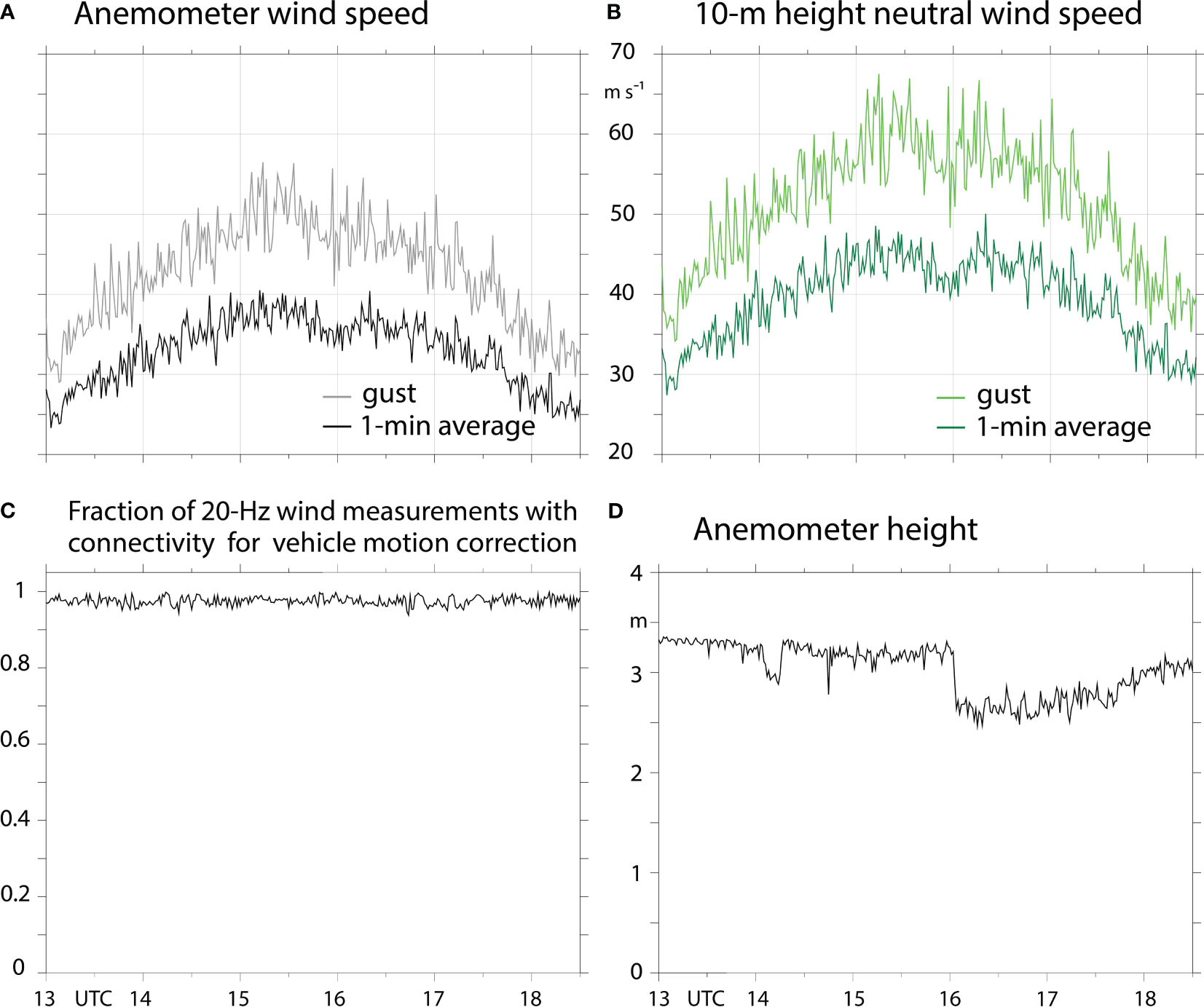
Figure 1 (A) One-minute averaged, earth-relative wind speed and gusts measured by the anemometer; (B) same as (A) except adjusted to 10-m height neutral wind speed using the COARE 3.5 algorithm; (C) fraction of 20-Hz wind measurements with Inertial Mesaurement Unit (IMU) and Global Navigation Satellite System (GNSS) connectivity needed to remove vehicle motion effects from the wind measurements; (D) height of the anemometer above the vehicle water line. The time interval shown includes the period over which 1-min averaged hurricane strength winds (>33 m/s) at 10-m height were measured by the vehicle (i.e., 1316–1824 UTC).

Relative humidity and air temperature sensors were installed 2.3 m above the water line. A low bias in relative humidity, identified through buoy comparisons at the start of this mission and with similarly equipped vehicles in the tropical Pacific, was corrected by adding 4%, up to a maximum of 100%. Conclusions are not affected by this adjustment. Surface pressure was measured at 0.2 m height and Photosynthetically Active Radiation (PAR) at 2.6 m height. Incoming solar radiation was estimated from PAR (García-Rodríguez et al., 2020) and was found to be greatly reduced, compared to clear-sky daytime conditions, under convective clouds in the hurricane’s eyewall. Near-surface seawater temperature and conductivity were measured 1.5 m below the vehicle water line. The 1.5 m temperature will be referred to as SST hereafter and was found to be in close agreement with underwater glider (Eriksen et al., 2001; Goni et al., 2017; Testor et al., 2019) temperatures averaged over 0–10 m depth when the saildrones and gliders were co-located (< 10 km apart) north and south of Puerto Rico (Supplementary Text 1). See Zhang et al. (2023) for a discussion of how near-surface glider and saildrone temperature and salinity differences varied with vehicle separation. Saildrone SST also showed close agreement with independent measurements from thermistors mounted on the saildrone hull at 0.5 m depth in other missions that sampled TCs, supporting the accuracy of saildrone SST in high-wind, overcast conditions (Supplementary Text 1 and Supplementary Figure 1). RTOFS simulated little temperature variation between 0 and 2 m depth during our study period (within 0.01°C on 30 September) implying that saildrone SST offers an appropriate comparison to RTOFS SST for this analysis. The sensor-resolution (1 Hz) conductivity measurements collected near the core of Sam showed negative spikes that may have been caused by air bubbles entering the conductivity cell. The spikes were flagged by comparison with valid measurements apparent in each 1-minute sampling period and removed prior to calculating the 1-minute average salinity used in this study. Ocean currents in the upper 100 m were measured by an Acoustic Doppler Current Profiler (ADCP) mounted at 1.9 m depth. Other saildrone measurements include surface wave height and period. A schematic showing sensor location on the vehicle is provided in Figure 2. The complete sensor list is provided in Supplementary Table 1.

Figure 2

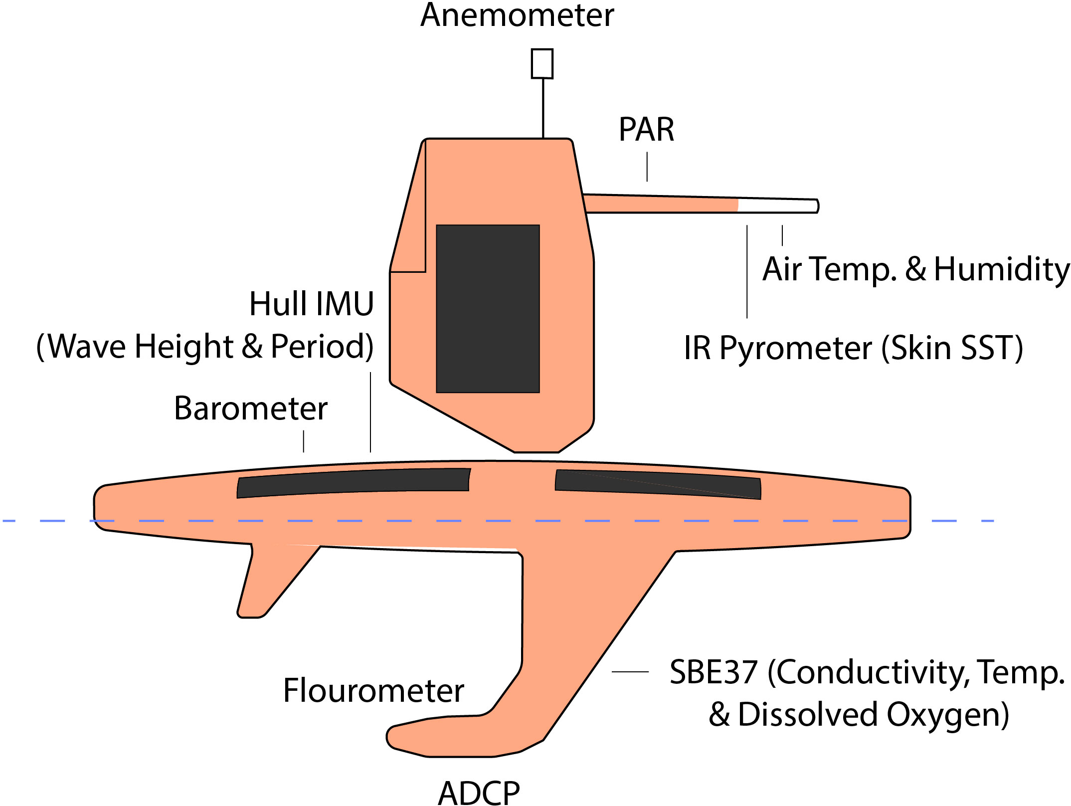
Figure 2 Hurricane-wing saildrone sensor schematic. See Supplementary Table 1 for sensor make and model, installation height, sampling frequency and nominal accuracy.

2.2 Other observations

Upper-ocean temperature and salinity profiles were provided by Argo float-dive numbers 5906436-015, 6902766-165, and 4902326-116 (Figure 3). Uppermost measurements were between 0.2 m and 4.0 m depth, with vertical resolution thereafter between 1 m and 2 m. Profile dates, locations, times and distances to the hurricane intercept and closest distance to the track of the storm center are listed in Table 1. An Airborne Expendable Bathy Thermograph (AXBT) was deployed ahead of Sam at 1120 UTC 29 September, approximately 200 km east of Argo profile 6902766-165 (Table 1; Figure 3).

Figure 3

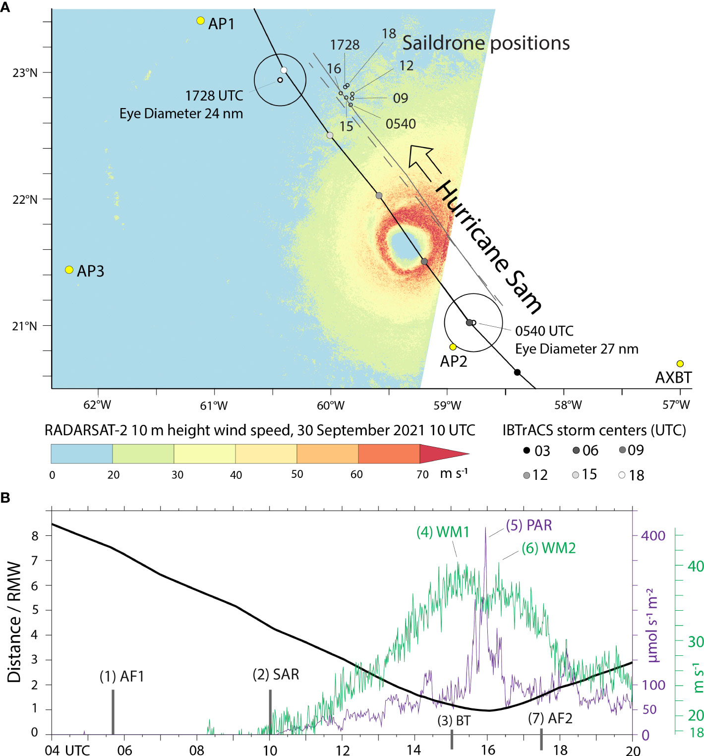
Figure 3 (A) SAR 10-m height wind speed field from RADARSAT-2. The SAR measurement occurred ~6 hours before SD-1045 was closest to the center of Hurricane Sam, when Sam was moving toward the saildrone at 6.32 m s^-1. SD-1045’s positions at the listed times are shown by small, open black circles. The black line intersecting the figure is the path of Sam’s center according to IBTrACS, with its 3-hourly center position shown in color coded circle markers. The gray lines to its right show the extent of the RMW estimated using aircraft (dashed) and IBTrACS (solid) center fixes. The eye diameters (black circular contours) and storm center positions at 0540 and 1728 UTC 9/30 (small white circles) were provided by aircraft reconnaissance. The locations of Argo Profile (AP) 1, 2 and 3, and the 1120 UTC 9/29 AXBT are shown with small yellow circles. (B) The black line shows the distance between SD-1045 and the IBTrACS center of Sam on 9/30, normalized by the RMW (30km). The times of other relevant measurements are marked, as follows: 1) AF1 = First Air Force storm center fix; 2) SAR = collection time of winds shown in panel (A); 3) BT = Infrared Brightness Temperature shown in Figure 4; 4) WM1 = First saildrone wind speed maximum; 5) PAR maximum; 6) WM2 = Second saildrone wind speed maximum; 7) AF2 = Second Air Force storm center fix. The green and purple lines show the 1-minute saildrone wind speed and PAR, respectively.

Table 1

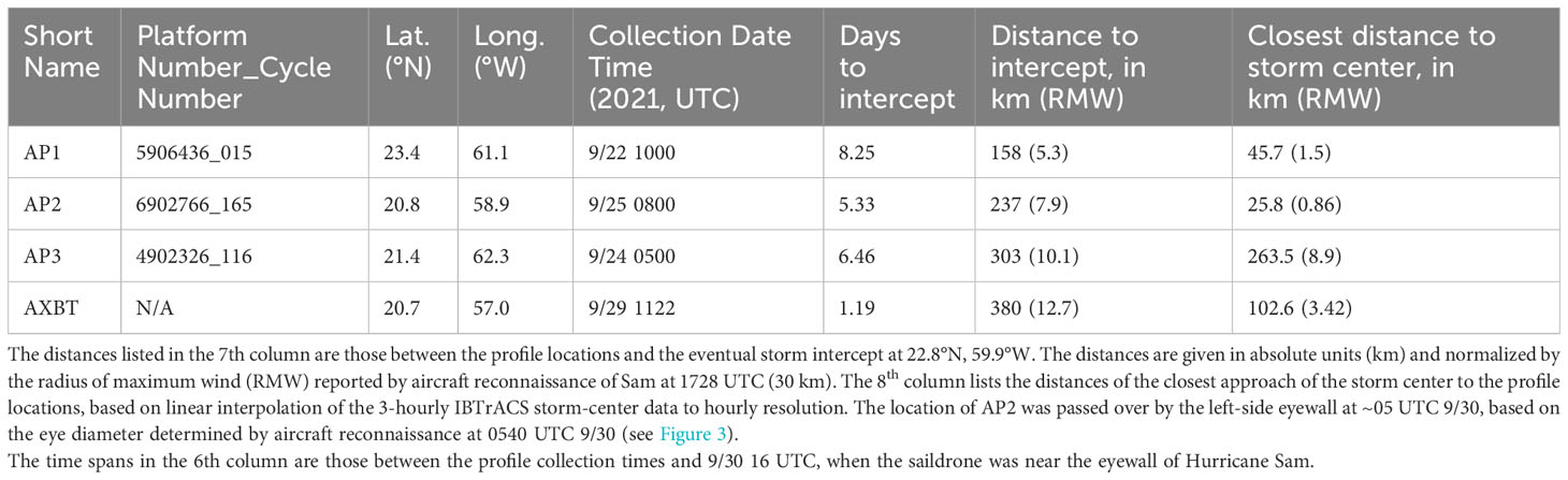
Table 1 Locations of nearest, pre-storm Argo Profile (AP) and Airborne Expendable Bathy Thermograph (AXBT) profiles.

Figure 4

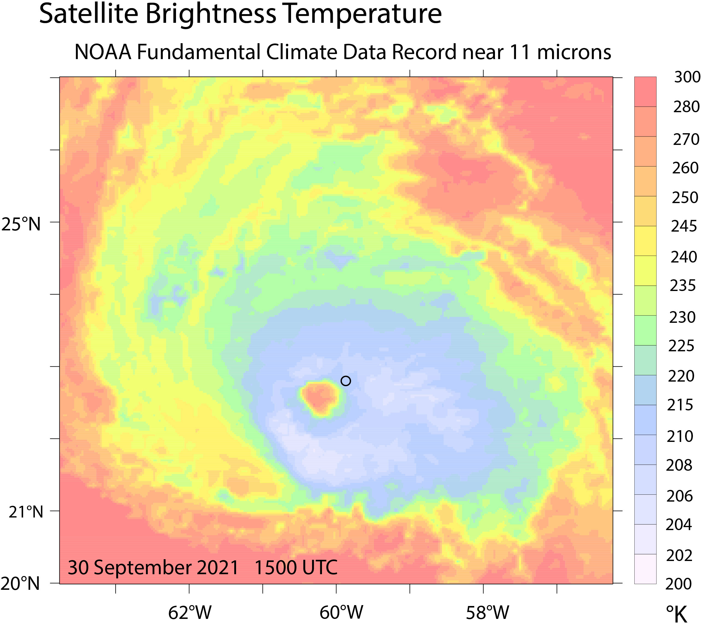
Figure 4 Geostationary infrared radiation (IR) channel brightness temperature, valid 15 UTC, 30 September 2021. The circle shows the location of SD-1045 in Hurricane Sam at this time.

Hurricane track information was provided by the International Best Track Archive for Climate Stewardship (IBTrACS; Knapp et al., 2018) project. IBTrACS combines 6-hourly records from the North Atlantic Hurricane Database version 2 (HURDAT2; Landsea and Franklin, 2013) with intermediate advisories to produce a 3-hourly record. Additional storm track information was provided by United States Air Force aircraft reconnaissance (Figure 3).

SST gradients in the vicinity of SD-1045 were estimated using Group for High Resolution Sea Surface Temperature (GHRSST; version 4.1) and Optimum Interpolation Sea Surface Temperature (OISST; version 5.1) data. These daily SST data sets were made available by NASA Jet Propulsion Laboratory (JPL) and Remote Sensing Systems (RSS), respectively. GHRSST and OISST have been used to estimate the effects of SST advection and SST response in the hurricane environment previously (e.g., Rudzin et al., 2019; Sun et al., 2021). OISST has a spatial resolution of 0.25° latitude by 0.25° longitude. GHRSST has a finer spatial resolution of 1 km. GHRSST, however, has been shown by Jaimes de la Cruz et al. (2021) to have an in-storm SST bias up to 0.6°C, which is close to the SST bias between the saildrone and the model output (RTOFS and HWRF) that we investigate (~0.5°C). The spatial resolution of GHRSST is also on the order of the distance that the saildrone drifted during storm overpass (as discussed below), meaning that evaluation of the effects of SST gradient advection relative to the saildrone are, at best, at the detection limit of the available SST gradient information. Hence, the uncertainty associated with the gridded SST product likely prevents a high-confidence assessment of the effects of the advection of the SST gradient on the saildrone SST. While we acknowledge this limitation, we have nonetheless chosen to offer such an assessment in Section 3.4 with the qualification that it should not be considered main support for the conclusions, but rather, complementary to the main analyses presented in Sections 3.2 and 3.3.

2.3 Air-sea flux calculations

Air-sea momentum (τ), latent (Q_l) and sensible (Q_s) heat fluxes were calculated in parameterized form (Cronin et al., 2019):

$${\tau }_x= \rho C_d S dU, {\tau }_y= \rho C_d S dV$$

$$Q_l= \rho L_v C_e S dQ$$

$$Q_s= \rho c_p C_h S dT$$

using the Coupled Ocean-Atmosphere Response Experiment (COARE) 3.5 algorithm (Fairall et al., 2003; Edson et al., 2013). τ_x and τ_y are the zonal and meridional components of wind stress; ρ is air density. dU and dV are the zonal and meridional components of the surface-relative wind vector, calculated by subtracting the uppermost (6 m depth) ADCP current vector from the geo-relative wind vector. S is surface-relative wind speed. dQ and dT are the near-surface ocean to atmosphere differences in specific humidity and temperature (SST). Specific humidity is assumed to be very near its equilibrium value at the ocean surface and is, thus, a function of SST. L_v is the latent heat of vaporization, and c_p is specific heat at constant pressure. C_d, C_e and C_h are the exchange coefficients for momentum, latent and sensible heat flux. Little observational evidence is available to evaluate coefficient behavior for S > 25 m s^-1. Therefore, for S > 25 m s^-1, we assumed that surface roughness length saturated at the mean value predicted by COARE 3.5 for 23< S< 25 m s^-1, resulting in C_d ~3.0×10^-3 for S > 25 m s^-1. This assumption follows Ricciardulli et al. (2022) and is motivated by the Black et al. (2007) and Chen et al. (2013) findings that C_d is invariant with wind speed above 25-30 m s^-1. Following Black et al. (2007), we estimate air-sea enthalpy flux as the sum of surface latent and sensible heat flux. The resulting saildrone enthalpy flux is similar to the Coupled Boundary Layer Air-Sea Transfer (CBLAST) parameterization (Chen et al., 2007).

2.4 Operational hurricane forecast models

HWRF is an atmosphere-ocean model developed for TC applications (Biswas et al., 2018). In 2021, 3-D temperature and salinity fields from daily RTOFS nowcasts (a.k.a. analyses) were used to initialize the ocean component of HWRF, namely the Princeton Ocean Model. RTOFS was itself initialized with fields from the Navy Coupled Ocean Data Assimilation (NCODA) system, which used 3-D multi-variate data assimilation (Cummings, 2005) to incorporate observations such as ocean temperature and salinity profiles from Argo floats. RTOFS incorporates momentum, radiation, and precipitation flux forcing from operational NOAA Global Forecast System (GFS) fields, and the resulting 3-D RTOFS temperature and salinity fields valid each day at 00 UTC were used to initialize the four daily HWRF runs (00 UTC, 06 UTC, 12 UTC and 18 UTC; see Biswas et al., 2018 for more information about the operational HWRF system).

The RTOFS analysis surface salinity and temperature data used in this study has hourly and 7-9 km horizontal resolution over our study area (Mehra et al., 2015). The RTOFS analysis subsurface variables have 6 hourly resolution and vertical grid cells spaced 2 m apart from 0-12 m, 5 m from 15-50 m, 10 m from 50-100 m, and 25 m from 100-150 m depth.

Two operationally-issued HWRF runs, initialized at 06 UTC on September 29th and 30th (HWRF_0929 and HWRF_0930, hereafter) were obtained following the mission. These initialization times occurred 10 and 34 hours before the saildrone was closest to the center of Sam at ~ 9/30 16 UTC (Section 3.1). SST change near the core of TCs is known to be largely driven by the wind-driven entrainment of sub-surface water into the mixed layer (Price, 1981; Black et al., 2007). It follows that coupled-model simulation of TC-driven SST changes depend on the accuracy of the near-surface wind fields. HWRF near-surface wind and track forecasts have generally demonstrated improved accuracy with decreasing lead time over the 10 - 34 hour range (see Figures 5 and 6 of Bachmann and Torn, 2021) and tend to offer improved accuracy at this range (10 - 34 hours) compared runs initialized two, or more, days out. Thus, by evaluating HWRF results at relatively short lead time, we are evaluating the model nearer to the time it was last provided observations and when we expect its ability to simulate in-storm SST change to be high, compared to longer-lead forecasts.

The HWRF data obtained for this study has 1.3-2.4 km horizontal and hourly resolution. To facilitate model evaluation, the 1-minute saildrone measurements were averaged to the hourly model time grid and the model output was linearly interpolated to the hourly mean saildrone position.

2.5 1-Dimensional ocean model experiments

Forced 1-Dimensional (1D) ocean model experiments were performed to evaluate the effects of alternately initializing the model ocean with salinity and temperature from the nearest Argo profiles, compared to corresponding RTOFS profiles. The experiments were performed using the K-Profile Parameterization model (KPP; Large et al., 1994) implemented in the General Ocean Turbulence Model (GOTM; Burchard et al., 1999). Base-case surface forcing was primarily calculated from hourly averaged saildrone observations and the COARE 3.5 algorithm, with downward solar radiation estimated from saildrone PAR measurements, following García-Rodríguez et al. (2020). The exceptions were precipitation minus evaporation, which was set to 0 following RTOFS, and downward longwave radiation; SD-1045 did not measure precipitation or downward longwave radiation, which was obtained by linearly interpolating GFS data to the saildrone location. GFS was used to maintain consistency with RTOFS. The 1D model resolved the 0 to 300 m depth range with 1-m resolution. Experiments were initialized at 20 UTC the day prior to intercept (29 September) and produced hourly output. The sensitivity of the results to the choice of critical Richardson number (Ric) was tested by using three different settings; the theoretical value (Ric = 0.25), Ric = 0.235 and Ric = 0.3. The use of Ric = 0.235 and Ric = 0.3 was motivated by comments from a reviewer and the study of Reichl et al. (2016), which compared KPP and large eddy simulation (LES) results in TC conditions and found that, at 1-m vertical resolution (as used herein), KPP with Ric = 0.235 best matched results from LES run without the effects of Langmuir turbulence, and KPP with Ric = 0.3 produced SSTs that tracked the LES experiments that included Langmuir turbulence.

A second set of tests were performed to evaluate the sensitivity of KPP results to variations in the wind speeds used to calculate the surface forcing. In this case, the KPP model was forced with 6 different sets of surface forcing. Two were identical to the base case, except with in-storm wind speeds adjusted by -10% and +10% to evaluate the effects of the 10% in-storm wind speed uncertainty suggested by the findings of Ricciardulli et al. (2022). Two other experiments were forced with in-storm wind speeds increased by up to +25% and +50%. These larger adjustments were applied to evaluate scenarios in which the saildrone happened to transect the storm closer to the point, anywhere in the storm, where maximum wind speeds occurred. Finally, two other experiments were forced with surface fluxes sampled from HWRF_0929 along two saildrone transects through the storm. These transects are described in Section 3.3. Because results from the first set of tests (Ric sensitivity) showed that the differences in KPP SST between Argo versus RTOFS initialization were insensitive to the choice of Ric (Section 3.3), one Ric setting (Ric = 0.25) was used for the second set of wind speed sensitivity tests.

3 Results

3.1 Storm intercept

Hurricane Sam’s track was forecasted by GFS as early as 21 September when SD-1045 was at ~22.3°N, 61.4°W. Routed to intercept Sam, SD-1045 traveled 140 km east-northeast over the next 5 days at an average speed of 0.58 m s^-1. The saildrone reached its preliminary intercept waypoint on 26 September, leaving 4 days to fine-tune position as subsequent storm track forecasts became available, which typically become more reliable as lead time decreases and a TC forms.

Radarsat-2 synthetic aperture radar (SAR) measurements offered a view of near-surface wind speed at 10 UTC, ~6 hours before the saildrone was closest to the center of Sam (Figure 3). At the SAR collection time, Sam was centered at 21.68°N, 59.33°W, still 130 km from the saildrone’s location, moving in direction 324° (northwest toward the saildrone) at a speed of 6.3 m s^-1 based on IBTrACS. The eventual minimum distance between the saildrone and the storm center was 29 km at 1603 UTC based on interpolation of IBTrACS 3-hourly storm center estimates, and 35 km at 1535 UTC based on interpolation of the two storm center fixes provided by aircraft reconnaissance at 0540 UTC and 1728 UTC 30 September (Figure 3B).

Aircraft reconnaissance determined the location of maximum winds in the northeast storm sector to be 30 km from the storm center at 1728 UTC (Figure 3A). Assuming that a radius of maximum winds (RMW) of 30 km holds at the time the saildrone was closest to the storm center, the saildrone was then either within the RMW by 1 km based on IBTrACS, or 5 km beyond it based on linear interpolation of the 0540 UTC and 1728 UTC aircraft center fixes. The following examination of the character of the observations collected near the core of Sam offers more information about which parts of the storm were transected.

The maximum 1-minute averaged saildrone wind speed of 40.5 m s^-1 was recorded at 1512 UTC 30 September, with gusts to 52.11 m s^-1 (Figures 1A and 3B). A measured wind speed of 40.5 m s^-1 at 3.0 m height equates to a COARE 3.5 10 m-height wind speed of 47.16 m s^-1 (Figure 1B). Gusts reached 56.49 m s^-1 two minutes later. Wind speeds comparatively slowed between 1550 and 1610 UTC (32.93 to 36.24 m s^-1) before a second peak of 40.41 m s^-1 (2.5 m height) was observed at 1620 UTC. Adjusted to 10-m height, this second peak equates to 49.04 m s^-1.

Between wind speed peaks, PAR increased from an average of 80 μmol s^-1 m^-2 (1500-1520 UTC), to an average of 234 (1550-1610 UTC), with a peak of 417.0 μmol s^-1 m^-2 at 1557 UTC (Figure 3B). From 1630 to 17 UTC, PAR remained below 100 μmol s^-1 m^-2. This was during daytime, when measurements under clear skies would have been much larger (for example, PAR remained above 1785 μmol s^-1 m^-2 from 15 to 17 UTC on 28 September). Thus, the comparative reduction in PAR during the storm intercept was likely caused by convective cloud cover in the eyewall, and the peak at 1557 UTC was indicative of a partial cloud break. That this cloud break occurred near the time that the vehicle was closest to the storm center (1535 UTC based on aircraft; 1603 UTC based on IBTrACS) and between peaks in wind speed (Figure 3B) suggests that the saildrone collected measurements between the eyewall and eye, after penetrating the radius of maximum winds. This is consistent with the storm-relative vehicle tracks presented as part of the HWRF simulation analysis in the following section (c.f. Figures 6B, C).

3.2 Observed upper-ocean response to hurricane Sam

On 30 September 2021, observed SST held near 28.8°C from 00 to 0930 UTC as observed wind speed rose from 8.8 to 16.9 m s^-1 (Figure 5A). SST increased by 0.2°C from 0930 to 14 UTC, reaching 29.0°C as wind speed rose above 30 m s^-1. Similar SST changes relative to a TC center were observed in Sraj et al. (2013). SST remained above 28.85°C through 1512 UTC as wind speed peaked for the first time and remained above 28.5°C through 17 UTC.

Figure 5

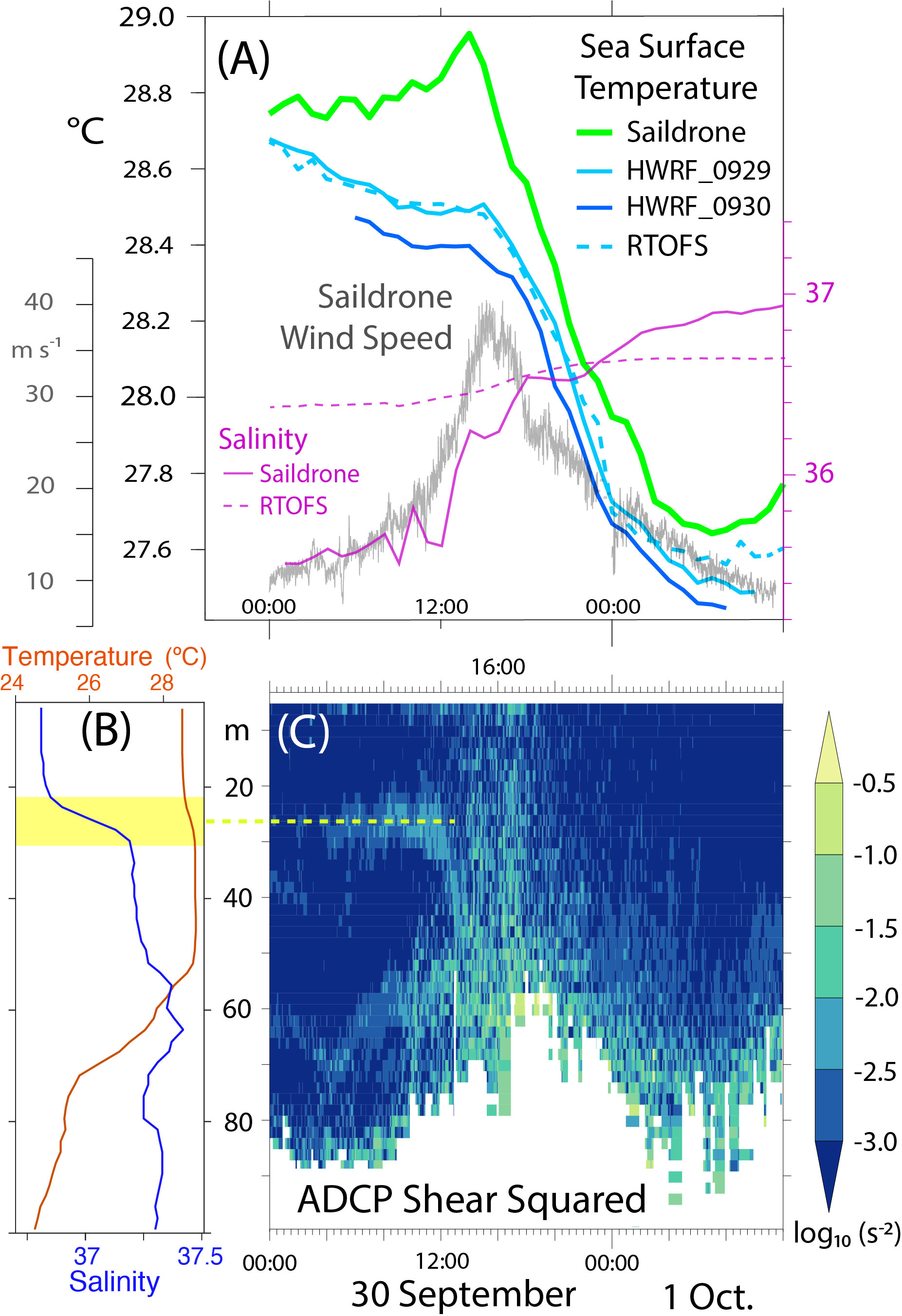
Figure 5 (A) Saildrone SST (green), wind speed (gray) and salinity (purple) in Hurricane Sam, with SST from RTOFS (dashed, light blue), HWRF_0929 (light blue) and HWRF_0930 (dark blue). Sea surface salinity from RTOFS is drawn with a dashed purple line. (B) Upper-ocean temperature (red) and salinity (blue) from the nearest Argo profile. Yellow shading highlights the halocline discussed in the text. (C) Vertical ocean current shear squared; dashed yellow line marks the central halocline depth.

RTOFS SST at the saildrone location was in relatively close agreement with the saildrone measurements at the start of the day (-0.07°C model bias at 00 UTC), but cooled during the first half of the storm, contrary to observations. The model cold bias reached 0.47°C at 14 UTC. The other two largest cold biases (~0.4°C) occurred at 13 and 15 UTC.

SST predicted by HWRF_0929 was quantitatively similar to RTOFS. For example, the peak HWRF_0929 bias of -0.46°C at 14 UTC is within 0.01°C of the RTOFS bias at that time (Figure 5A). HWRF_0930 results are also qualitatively similar to RTOFS, except cooler by ~0.1°C. This suggests that the initial conditions provided by RTOFS to HWRF largely controlled the in-storm SST behavior simulated by the ocean component of HWRF.

Effects of model storm track error were evaluated by adjusting the vehicle-sampling transects to account for the differences between the HWRF-predicted and IBTrACS storm centers. This was done by adjusting the vehicle transect through the model storm by first calculating the time-dependent distances between the HWRF storm centers and those reported in IBTrACS, then subtracting those distances (linearly interpolated to hourly HWRF output resolution) from the saildrone positions used to sub-sample the HWRF_0929 and HWRF_0930 SST. In this way, the observed (saildrone-IBTrACS) relationship between storm center and vehicle location was replicated in the adjusted-transect HWRF sampling. The adjusted transects are illustrated in panels B and C of Figure 6 and produce similar SSTs to their unadjusted counterparts (Figure 6A), confirming that the cool bias in HWRF cannot be attributed to the model track errors.

Figure 6

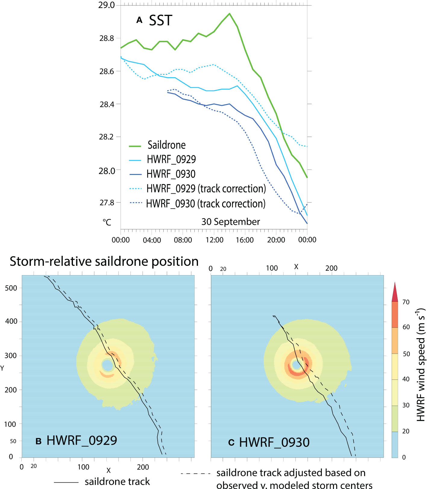
Figure 6 (A) SST measured by SD-1045 (green curve) and sampled at the saildrone location in HWRF_0929 (light blue) and HWRF_0930 (dark blue). The dashed SST curves were also produced by sampling HWRF_0929 and HWRF_0930, respectively, after adjusting the transect by subtracting the differences between the modeled storm centers and those reported in IBTrACS. The original (solid black curve) and adjusted (dashed black curve) saildrone transects are shown in panels (B, C).

The closest Argo float profile (AP1; 8.25 days and 158 km from intercept) reveals a halocline centered at ~25 m depth wherein salinity increases by 0.36 from 20 m (36.83) to 30 m (37.19; Figure 5B) and potential density increases by 0.169 kg m^-2. Temperature from the surface to 15 m depth is nearly constant at 28.51°C, but then increases by 0.31°C from 15 m to 30 m depth. Temperature remains above the mixed layer value of 28.51°C until 55 m depth, revealing a 40 m-thick temperature inversion. The maximum temperature was 28.88°C at 45 m depth. The closest AXBT (1122 UTC 29 September) also showed a temperature inversion centered around 30 m depth (Supplementary Figure 2).

The ADCP measurements reveal enhanced shear near the pycnocline from 04 to 13 UTC (Figure 5C). Evidently, a pycnocline at the saildrone’s location prevented storm-induced mixing from entraining much of the warm water below 30 m during this time. Enhanced shear from the surface to 60-m depth is evident after ~14 UTC, suggesting entrainment of deeper (warmer) water into the surface mixed layer began in earnest then. Consistent with this view, salinity measured by the saildrone rose ~1 unit from its 04 - 13 UTC average of 35.6 to a value of 36.5 at 1824 UTC, when hurricane-strength wind (10 m-height wind speed > 33 m s^-1) was last measured by SD-1045 (Figure 5A). The rise in RTOFS salinity during this time was much weaker than observed (c.f. dashed and solid magenta curves in Figure 5A).

These observational results suggest that vertical mixing was responsible for the maintenance and warming of SST through the first half of the storm. This hypothesis will be tested in a series of 1D ocean model experiments in the following section. The alternative hypothesis, that the mid-storm warming was caused by horizontal vehicle motion and advection of the SST gradient, will be evaluated in section 3.4.

3.3 1D Model ocean response

A series of 1D ocean model experiments was performed to isolate the impacts of upper-ocean initial conditions on the response to Sam. Two sets of experiments were conducted: in the first, ocean initial conditions were taken from one of the three nearest Argo profiles (AP1, AP2 and AP3, hereafter; see Table 1 and Figure 3A for profile locations). The other set was initialized with RTOFS profiles sampled at the model grid points and times closest to the actual Argo profiles. The same surface forcing was applied in each case.

Mid-storm surface warming, with amplitude and timing similar to observations, was simulated in the experiment initialized with AP1 (Figure 7A). The model in this case also simulated enhanced vertical ocean current shear between 20 m and 30 m depth from ~04 to 13 UTC, in qualitative agreement with the ADCP observations (c.f. Figure 5C and Supplementary Figure 3).

AP2 and AP3 also exhibit upper ocean haloclines and temperature inversions (Figure 8; black curves) but with somewhat different characteristics than AP1: AP2 has a thicker inversion than AP1 (5 to 65 m) and AP3 has a warmer maximum temperature (29.05°C at 30 m). The resulting differences in model output produce a spread in simulated SST that varies in time. The average spread is 0.12°C between 14 UTC and 16 UTC. Nonetheless, the Argo-initialized average (black curve in Figure 7A) resembles the AP1 case in that it exhibits mid-storm warming with similar amplitude and timing as the observations.

Figure 7

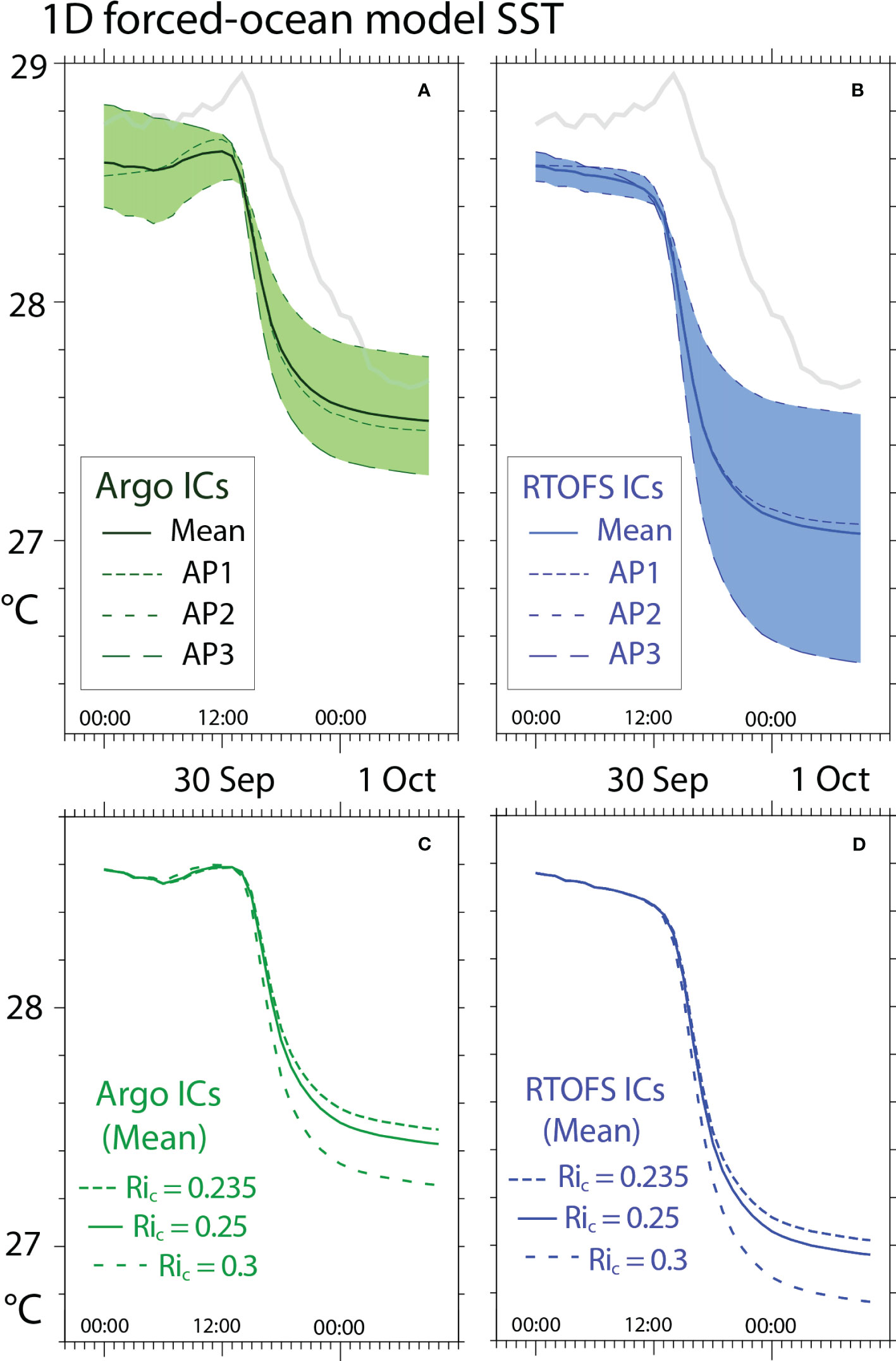
Figure 7 (A) SST from the Argo-initialized 1D ocean model experiments (Ric = 0.25) and saildrone measurements (light-gray curve). (B) Same as (A), except RTOFS-initialized. (C) The mean SST from panel (A) and mean SSTs from Argo-initialized runs with Ric = 0.235 and Ric = 0.3. (D) Same as (C), except RTOFS-initialized.

Figure 8

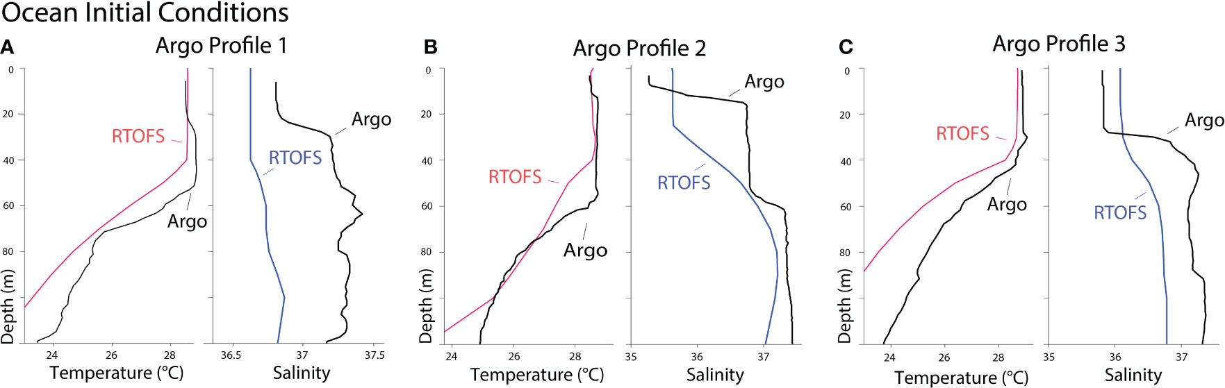
Figure 8 (A) AP1 upper-ocean temperature (left) and salinity (right). (B) same as (A), except for AP2. (C) Same as (A) except for AP3.

The average model result is a few tenths °C cooler than the observations during the first half of the storm (Figure 7A). This discrepancy may be due to spatial and temporal upper ocean variability (Ryan et al., 2015; Morrison et al., 2016) unresolved by profiles collected 5-8 days prior to, and 150-300 km away from the storm intercept.

Similar mid-storm warming is produced in the Argo-initialized average regardless of which Ric was used (Figure 7C). The amount of SST cooling seen during the second half of the storm shows a more noticeable dependence on Ric. For example, KPP SST at 18 UTC is 0.05 °C warmer with Ric = 0.235, and 0.15 °C cooler with Ric=0.3, than the Ric = 0.25 results. The signs of these later changes in SST are unsurprising considering that less shear is needed to decrease the Richardson number (ratio of buoyancy divided by vertical shear) below a larger critical value and that, by this point in the experiment, the vertical mixing is (finally) entraining cooler water into the mixed layer. The more salient question here is how the choice of Ric affects the Argo versus RTOFS experiments. This will be discussed momentarily.

The RTOFS-initialized experiments start, on average, with nearly the same SST as the mean of the Argo-initialized experiments and closely track the Argo case over the first hours of the run (their mean difference is only 0.016°C during 00 - 04 UTC; c.f. solid-black lines in Figures 7A, B). Unlike the Argo case, however, the RTOFS case does not warm during the storm. Rather, it cools as the storm approaches, leading to a cold bias, relative to Argo-initialization, that reaches ~0.4°C near the time of maximum winds (-0.40°C at 16 UTC; -0.42°C at 17 UTC). A larger net cooling is also seen in the second half of the storm in the RTOFS case.

Using the smaller (0.235) and larger (0.3) Ric values affected the RTOFS and Argo initialized experiments similarly (c.f. Figures 7C, D), with Ric=0.235 and Ric = 0.3 runs both showing small effects in the first compared to the second half of the storm. The key result in the second half is that the difference in SST caused by Argo versus RTOFS initialization proved to be similar regardless of which Ric was used. This holds during the few-hour interval bracketing the time that maximum winds (hence, maximum enthalpy fluxes) were observed by the saildrone. For example, the Ric = 0.235 and Ric = 0.3 experiments yielded RTOFS-initialized cold SST biases that, averaged 15-17 UTC, were within 1% and 2% of the Ric = 0.25 results, respectively. Evidently, the upper ocean temperature and salinity biases in RTOFS cause similar cold biases in KPP SST throughout the range of Ric values evaluated previously by Reichl et al. (2016) for use in TC simulation.

Sensitivity experiments revealed that similar SST biases (-0.37°C to -0.41°C) occurred in the RTOFS- compared to Argo-initialized runs regardless of which set of surface fluxes was applied (Supplementary Figures 4–6). The cool SST bias of ~0.4°C can therefore be attributed to the RTOFS ocean initialization. Comparisons of the corresponding Argo and RTOFS initial conditions highlight reasons why the RTOFS-initialized runs cool more readily than the Argo runs: the RTOFS profiles do not exhibit the temperature inversions or degree of salinity stratification evident in the Argo observations (Figure 8; red and blue compared to black curves). In the AP1 case, for example, RTOFS has virtually uniform temperature from the surface to the start of the thermocline and lacks the halocline evident in the measurements between 20 and 30 m depth (Figure 8A).

3.4 Horizontal advection

This section investigates the possibility that a combination of saildrone movement relative to the horizontal SST gradient and advection of the SST gradient past the saildrone by the local surface current caused the maintenance and warming of SST observed by SD-1045 during the approach of hurricane Sam.

To estimate the effects of vehicle movement on the saildrone SST measurements, we subsampled the GHRSST and OISST fields based on 1-minute SD-1045 position during its intercept of Sam. We focused on results from gridded-product SST data valid for 27 September because that was the day when the last pre-storm, 1-km horizontal resolution (relatively high resolution) satellite-based SST measurements were included in GHRSST in the vicinity of the intercept. The results of sampling the gridded SST products at the saildrone position are shown in Figure 9. From the time SD-1045 reached its pre-storm waypoint at ~09 UTC to the time that 1-minute SST peaked at ~14 UTC there is not much change in the SST caused by saildrone movement relative to the background SST gradient (dashed blue curve in Figures 9A, B). This is in part because the saildrone did not move very far during this time interval. For example, the saildrone had a net displacement of only 1.2 km between 09 and 14 UTC (Supplementary Figure 7) and stayed within 5 km of its 09 UTC location during this time. Thus, there would have needed to be a rather strong SST gradient in this region to cause the observed warming, and such a gradient is not evident in the available gridded SST data.

Figure 9

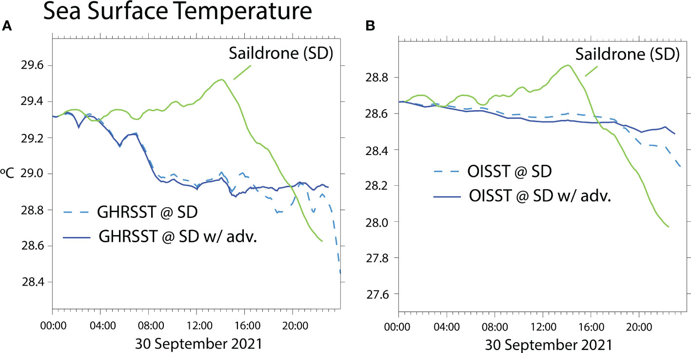
Figure 9 (A) The dashed blue curve shows the result of sampling pre-storm GHRSST data (valid 27 September) at the saildrone location to estimate the effects of vehicle motion on the saildrone SST measurements. The solid blue curve shows the result of adding the estimated effects of advection of the SST gradient past the saildrone location. Saildrone SST (green curve) has been overlaid with an offset that makes it initially (00 UTC) match the blue curve. The offset was applied to facilitate comparison. (B) Same as (A) except based on OISST.

We also estimated the change in temperature due to advection of the local SST gradient using the same GHRSST and OISST gridded-products discussed above and the uppermost (6m depth) ADCP current measured by the saildrone. The time-integral of this temperature advection term has been added to the gridded-product SST results in Figure 9 (solid-blue curves). Inclusion of this term does not change the result that the warming observed during the storm cannot be explained by the estimated effects of vehicle motion and temperature advection. For completeness, we repeated this analysis using SST gridded-products valid for the 28th and 29th of September and found qualitatively similar results (i.e., little SST change due to vehicle motion and horizontal temperature advection from 09 - 14 UTC; not shown). Gridded SST data for the 30th was not considered because of the likelihood that they incorporated in-storm and post-storm measurements that would be substantially altered by the storm overpass relative to the period of main interest here (i.e., storm approach to mid-overpass).

3.5 Enthalpy flux

To quantify the impacts of the operational RTOFS and HWRF SST biases on the estimation of air-sea heat fluxes, we compared four sets of enthalpy fluxes. In the first, the enthalpy flux is calculated using saildrone observations of wind, SST, air temperature and relative humidity. The other three sets use the same meteorological parameters, but substitute RTOFS, HWRF_0929 or HWRF_0930 output for the observed SST.

Saildrone SST produces the largest ocean-to-air difference in specific humidity (Δq) and temperature (ΔT) and, therefore, the largest enthalpy flux (Figure 10A). Using simulated SST reduces the flux by up to 120-160 W m^-2, depending on whether RTOFS, HWRF_0929 or HWRF_0930 is chosen. HWRF_0930 exhibits the largest surface cold bias and, therefore, the largest enthalpy flux bias (Figure 10B). Averaged between the peaks in wind speed at 1512 UTC and 1620 UTC, the use of forecasted rather than observed SST produces a 12-17% drop in enthalpy flux. Averaging over other high-wind intervals yields similar results (e.g., 1430-1630 UTC also yields a 12-17% drop). Together, these results suggest that the model surface temperature errors, which peaked near the time of maximum winds, likely caused surface enthalpy flux to be reduced by 12-17% in the HWRF simulations.

Figure 10

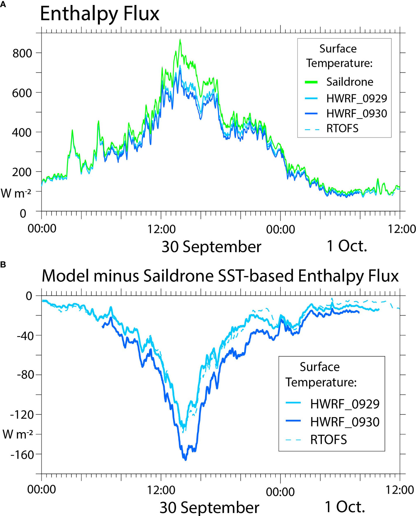
Figure 10 (A) Surface enthalpy flux calculated using observed atmospheric parameters and SST from saildrone observations (green curve), HWRF_0929 (light-blue curve), HWRF_0930 (blue curve) and RTOFS (dashed curve). (B) Difference between the observational and model results shown in Panel (A).

3.6 Potential intensity

A theoretical framework for relating air-sea enthalpy flux (F_k) in the eyewall of a TC to its potential intensity has been proposed by Emanuel (2003) and evaluated by D’Asaro et al. (2007) using the formulation:

$$V_{max}^3\approx F_k \frac{T_s-T_o}{ \rho C_d T_o}$$

Here, inputs of $\rho$ in kg m^-3 and SST (T_s) and tropospheric outflow temperature (T_o) in Kelvin yield maximum sustained 10-m wind speeds (V_max) in m s^-1. We estimate T_o = 200°K based on the minimum infrared radiation-channel brightness temperatures (Knapp, 2008) seen in Sam around the time maximum winds were measured by SD-1045 (15 UTC; Figure 4). The 12-17% drop in F_k caused by substituting forecasted for observed surface temperatures equates to reductions in V_max of 4-6% from the observation-based value of 49.5 m s^-1.

Pasch and Roberts (2022) report that, after reaching maximum strength on 26 September, Sam weakened during an eyewall replacement cycle on the 27^th and 28^th and then moderately restrengthened on 30 September and 1 October (c.f. Figure 11). Specifically, from the day prior (29 September) to the day after (1 October) the intercept, the V_max of Sam increased by 13% based on IBTrACS. This constitutes an average daily increase of ~6.5%, which is close in magnitude to the drop in V_max theoretically attributable to the near-eyewall cold biases in HWRF SST. These findings motivate the hypothesis that one reason for the lack of a multi-day increase in intensity in the HWRF_0929 and HWRF_0930 forecasts is that the cold biases in HWRF SST unrealistically limited the enthalpy fluxes simulated in HWRF near the eyewall.

Figure 11

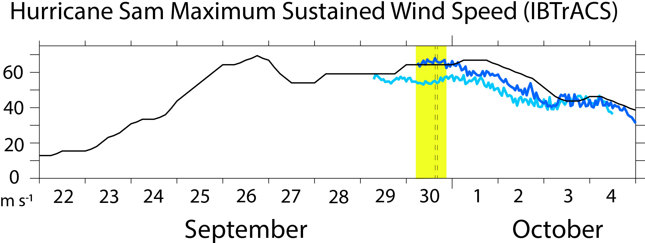
Figure 11 (A) Hurricane Sam maximum sustained wind speed at 10 m height from IBTrACS (black curve), HWRF_0929 (light blue curve) and HWRF_0930 (dark blue curve). The dashed vertical lines denote the SD1045-Hurricane Sam intercept period between wind speed peaks. The yellow shading is in between the times at which the center track of hurricane Sam was closest to the locations of AP1 (45.7 km; Table 1) and AP2 (25.8 km).

This hypothesis assumes that the cold SST biases revealed by the near-eyewall saildrone measurements were representative of model biases near the core of Sam during its restrengthening on 30 September and 1 October. Although having only a single vehicle transect limits our ability to assess the validity of this assumption, a couple of factors support the representativeness of the saildrone measurements in this case. One is that similar SST biases were produced in the 1D model experiments regardless of which set of surface fluxes were applied. This suggests that the development of a cold bias in HWRF SST depends less on the details of the in-storm surface fluxes than the lack, in the model system, of upper ocean salinity stratification and temperature inversions resembling the nearest Argo profiles. That the center of Sam passed<50 km from the locations of AP1 and AP2 on 30 September (at 21 and 05 UTC, respectively) supports the assumption that Sam encountered such upper-ocean conditions on the 30^th to the extent that the temperature inversions and the associated haloclines seen in the Argo measurements held from the time the profiles were collected to intercept (5-8 days). Efforts to improve our understanding of actual temporal and spatial variability of temperature inversions in TC prone regions (c.f., Mignot et al., 2012) would improve our ability to quantify this uncertainty, and by extension, the effectiveness of our observing system. This may provide fertile ground for future study.

3.7 Regional distribution of temperature inversions

To better understand the likelihood that a TC would encounter an upper-ocean temperature inversion elsewhere in the study region (i.e., away from the intercept), the 263 Argo profiles collected between 15 September - 31 October 2021, 13°N-30°N, and 70°W-50°W were evaluated. Inversions were identified by screening for subsurface temperatures that exceeded the 0 – 10 m depth average temperature by the 0.03°C uncertainty level, or greater. 29% (77 of 263) of the profiles in the study region exhibited inversions (Figure 12). The maximum subsurface temperature exceeded the 0 - 10 m average temperature by up to 0.75°C, with an average of 0.26°C over the 77 profiles with inversions. Evidently, the potential for TC-driven vertical mixing to cause SST warming was not unique to the Argo profiles nearest the saildrone intercept. This suggests that in-storm RTOFS and HWRF SST biases, like those identified here, may affect a substantial portion of TC simulations over the broader study region.

Figure 12

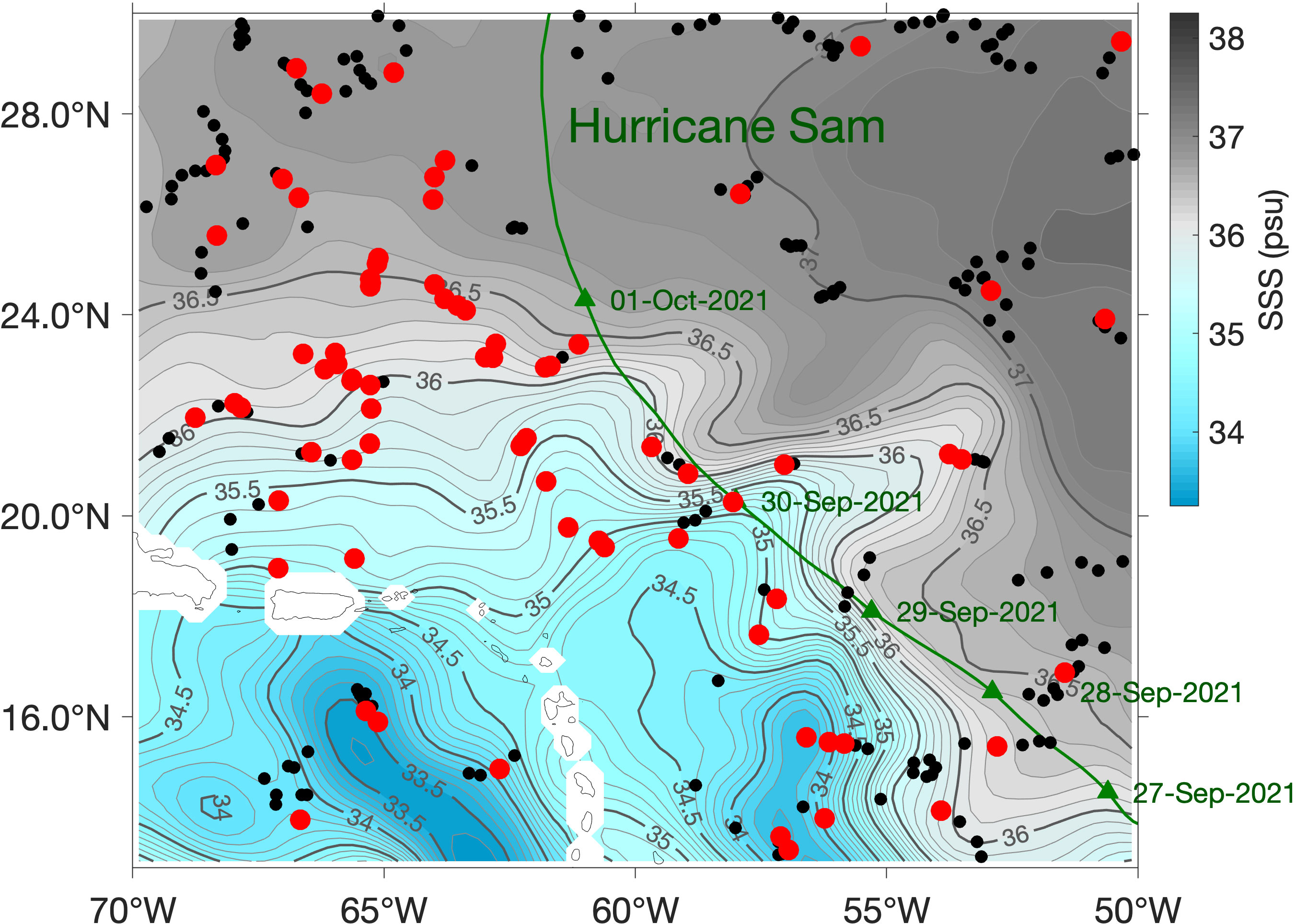
Figure 12 Argo float profiles with (red dots) and without (black dots) temperature inversions during 15 September 2021 – 31 October 2021. 29% (77 of 263) of the profiles in the study region exhibited inversions. The background shading shows Sea Surface Salinity (SSS) averaged for the same time period from the Multi-Mission Optimally Interpolated Sea Surface Salinity (OISSS) data set. The green line marks hurricane Sam’s path from IBTrACS.

4 Discussion

Storm intercept logistics, Radarsat-2 winds, IR brightness temperature from geostationary satellites and the character of the saildrone observations collected in Hurricane Sam led us to conclude that the saildrone traversed the northeastern-to-eastern eyewall of Sam, consistent with initial assessments of Foltz et al. (2022) and (Zhang et al. (2023). This part of the storm was targeted because it is where maximum surface wind speeds typically occur and, correspondingly, where positive feedbacks between wind speed and air-sea enthalpy flux typically extract the most energy for TC intensification (Emanuel, 2003).

Observed surface temperatures held steady or warmed ahead of the TC center and dropped by an atypically small amount in the rear region of the storm after the passage of the storm center (Price, 1981; Cione et al., 2000; LLoyd and Vecchi, 2011; Sraj et al., 2013; Zhang et al., 2017). RTOFS and HWRF predicted cooling throughout the storm, which increased their cold biases from initial magnitudes of ~0.1°C to a peak of ~0.5°C near the time that strongest winds were observed.

Pre-storm Argo profiles exhibited upper-ocean temperature inversions capped by haloclines that were not apparent in RTOFS. This discrepancy explains why surface temperature maintenance and warming was simulated in the Argo-initialized 1D ocean model experiments but was not simulated in the RTOFS-initialized cases.

The 1D-model mean surface temperature difference (Argo minus RTOFS) increased from ~0.0°C at the start to ~0.4°C mid-storm. Thus, the 1D experiments capture the surface temperature bias (0.5°C) identified by saildrone measurements near the eyewall once the initial biases (0.1°C operational; 0.0°C 1D) are considered. The ~0.5°C cold biases that developed near the eyewall in the HWRF forecasts (identified by the saildrone) can be primarily attributed to the lack of realistic, pre-storm, upper ocean structure in RTOFS (identified by Argo). This type of model validation demonstrates the potential utility of combining subsurface (Argo or glider) and near-surface (saildrone) monitoring in the hurricane environment.

The cold biases simulated in HWRF peaked near the eyewall, where they likely caused surface enthalpy flux to be reduced by 12-17%. This reduction accounts for a 6% reduction in potential intensity (Emanuel, 2003) compared to evaluation with observations. Hurricane Sam intensified by approximately this amount near the time it passed over the saildrone (Pasch and Roberts, 2022). HWRF failed to capture the observed multi-day intensification. We hypothesize that the pre-storm upper ocean structure contributed to the observed intensification, and thereby, the notable longevity of Sam. The absence of intensification in HWRF may be, at least in part, attributable to the lack of temperature inversions and haloclines in RTOFS initial conditions. Coupled model experiments, however, will be needed to validate this hypothesis.

Typically, the tropical ocean is stratified by temperature so that storm-driven vertical mixing cools SST (Price, 1981; Price et al., 1986), reducing the potential intensity of storms. Reduced cooling during storm overpass owing to salinity stratification has been documented previously and associated, in this part of the ocean, with freshwater input from the Amazon and Orinoco Rivers (Ffield, 2007; Balaguru et al., 2012; Reul et al., 2014; Rudzin et al., 2019).

Less attention has been paid to the implications of the upper-ocean conditions described here, in which a pre-storm halocline separates a warmer subsurface from a colder surface layer. The continuous saildrone observations of SST in Sam confirm that warming occurred near the eyewall, and our analysis clearly attributes this to the prevailing upper-ocean temperature inversion, which was not captured in RTOFS even though it was evident in the nearest Argo and AXBT profiles. Temperature inversions were evident in 29% of the Argo profiles collected in the broader study region implying that the potential for an approaching TC to drive surface warming via vertical mixing was not limited to the intercept vicinity. Together, these results suggest that enhancing the regional upper-ocean observing system and improving the fidelity with which the observations are assimilated into ocean data assimilation systems could directly benefit Atlantic and Caribbean TC intensity forecasts.

Data availability statement

The datasets presented in this study can be found in online repositories. Argo profile 4902326_116 data are available at https://www.ncei.noaa.gov/data/oceans/argo/gdac/aoml/4902326/profiles/, 5906436_015 available at https://www.ncei.noaa.gov/data/oceans/argo/gdac/aoml/5906436/profiles/ and 6902766_165 available at https://www.ncei.noaa.gov/data/oceans/argo/gdac/coriolis/6902766/profiles/.

Author contributions

AC: Writing – original draft, Writing – review & editing. HH: Writing – original draft. GF: Writing – original draft, Writing – review & editing. JZ: Writing – review & editing. CM: Writing – review & editing. CE: Writing – review & editing. CZ: Writing – review & editing. CMe: Writing – review & editing. DZ: Writing – review & editing. EM: Writing – review & editing. EC: Writing – review & editing. EB: Writing – review & editing. FB: Writing – review & editing. GG: Writing – review & editing. H-SK: Writing – review & editing. SC: Writing – review & editing. JT: Writing – review & editing. KB: Writing – review & editing. KO: Writing – review & editing. MM-C: Writing – review & editing. NL: Writing – review & editing. SC: Writing – review & editing. XC: Writing – review & editing.

Funding

The author(s) declare financial support was received for the research, authorship, and/or publication of this article. Funding was provided by the NOAA Office of Marine and Aviation Operations, Oceanic and Atmospheric Research Ocean Portfolio, Weather Program Office, Global Ocean Monitoring and Observation Program (http://data.crossref.org/fundingdata/funder/10.13039/100018302), Pacific Marine Environmental Laboratory (PMEL), and Atlantic Oceanographic and Meteorological Laboratory (AOML). Funding for SC was provided by the Office of Naval Research, grant number N0001417WX01401. This publication is [partially] funded by the Cooperative Institute for Climate, Ocean, and Ecosystem Studies (CICOES) under NOAA Cooperative Agreement NA20OAR4320271, Contribution No. 2022-1231. This is PMEL contribution #5431.

Acknowledgments

The notable longevity of Hurricane Sam was previously pointed out by Phil Klotzbach. The principal investigators responsible for the 3 Argo float profiles closest to the SD1045-Sam intercept are Steve Riser, Ken Johnson, Guillaume Maze and Dean Roemmich. The manuscript benefited from helpful conversations with D.E. Harrison and comments and suggestions from reviewers. The PyFerret program was used for analysis and graphics in this paper. PyFerret is a product of PMEL. PyFerret software and more information is available at http://ferret.pmel.noaa.gov/Ferret/. The authors also sincerely thank the team at Saildrone, Inc. who supported and made this mission possible, including founder Richard Jenkins, Julia Paxton and Kimberly Sparling.

Conflict of interest

The authors declare that the research was conducted in the absence of any commercial or financial relationships that could be construed as a potential conflict of interest.

The author(s) declared that they were an editorial board member of Frontiers, at the time of submission. This had no impact on the peer review process and the final decision.

Publisher’s note

All claims expressed in this article are solely those of the authors and do not necessarily represent those of their affiliated organizations, or those of the publisher, the editors and the reviewers. Any product that may be evaluated in this article, or claim that may be made by its manufacturer, is not guaranteed or endorsed by the publisher.

Supplementary material

The Supplementary Material for this article can be found online at: https://www.frontiersin.org/articles/10.3389/fmars.2023.1297974/full#supplementary-material

References

Bachmann K., Torn R. D. (2021). Validation of HWRF-based probabilistic TC wind and precipitation forecasts. Weather Forecasting. 36, 2057–2070. doi: 10.1175/WAF-D-21-0070.1

CrossRef Full Text | Google Scholar

Balaguru K., Chang P., Saravanan R., Leung L. R., Xu Z., Li M., et al. (2012). Ocean barrier layers’ effect on tropical cyclone intensification. Proc. Natl. Acad. Sci. U.S.A. 109, 14343–14347. doi: 10.1073/pnas.1201364109

PubMed Abstract | CrossRef Full Text | Google Scholar

Biswas M. K., Bernardet L., Abarca S., Ginis I., Grell E., Kalina, et al. (2018). Hurricane Weather Research and Forecasting (HWRF) Model: 2017 Scientific Documentation (No. NCAR/TN-544+STR). doi: 10.5065/D6MK6BPR

CrossRef Full Text | Google Scholar

Black P. G., D’Asaro E. A., Drennan W. M., French J. R., Niiler P. P., Sanford T. B., et al. (2007). Air-sea exchange in hurricanes: Synthesis of observations from the Coupled Boundary Layer Air-Sea Transfer experiment. Bull. Am. Meteorol. Soc 88 (3), 357–374. doi: 10.1175/BAMS-88-3-357

CrossRef Full Text | Google Scholar

Burchard H., Bolding K., Ruiz-Villarreal M. (1999). GOTM, a general ocean turbulence model. Theory, implementation and test cases (European Commission).

Google Scholar

Chen S. S., Price J. F., Zhao W., Donelan M. A., Walsh E. J. (2007). The CBLAST-Hurricane Program and the next-generation fully coupled atmosphere-wave-ocean models for hurricane research and prediction. Bull. Amer. Meteor. Soc. 88, 311–317. doi: 10.1175/BAMS-88-3-311

CrossRef Full Text | Google Scholar

Chen S. S., Zhao W., Donelan M. A., Tolman H. L. (2013). Directional wind-wave coupling in fully coupled atmosphere-wave-ocean models: Results from CBLAST-Hurricane. J. Atmos. Sci. 70, 3198–3215. doi: 10.1175/JAS-D-12-0157.1

CrossRef Full Text | Google Scholar

Cione J. J., Black P. G., Houston S. H. (2000). Surface observations in the hurricane environment. Mon. Wea. Rev. 128, 1550–1561. doi: 10.1175/1520-0493(2000)128.1550:SOITHE.2.0.CO;2.,/jrn

CrossRef Full Text | Google Scholar

Cronin M. F., Gentemann C. L., Edson J., Ueki I., Bourassa M., Shannon Brown S., et al. (2019). Air-Sea Fluxes with a focus on heat and momentum. Front. Mar. Sci. 6. doi: 10.3389/fmars.2019.00430

CrossRef Full Text | Google Scholar

Cummings J. A. (2005). Operational multivariate ocean data assimilation. Q. J. R. Meteorol. Soc 131, 3583–3604. doi: 10.1256/qj.05.105

CrossRef Full Text | Google Scholar

D’Asaro E. A., Sanford T. B., Niiler P. P., Terrill E. J. (2007). Cold wake of hurricane Frances. Geophys. Res. Lett. 34, L15609. doi: 10.1029/2007GL030160

CrossRef Full Text | Google Scholar

Domingues R., Kuwano-Yoshida A., Chardon-Maldonado P., Todd R. E., Halliwell G., Kim H. S., et al. (2019). Ocean observations in support of studies and forecasts of tropical and extratropical cyclones. Front. Mar. Sci. 6. doi: 10.3389/fmars.2019.00446

CrossRef Full Text | Google Scholar

Edson J. B., Jampana V., Weller R. A., Bigorre S. P., Plueddemann A. J., Fairall C. W., et al. (2013). On the exchange of momentum over the open ocean. J. Phys. Oceanogr. 43, 1589–1610. doi: 10.1175/JPO-D-12-0173.1

CrossRef Full Text | Google Scholar

Emanuel K. A. (1986). An air-sea interaction theory for tropical cyclones. Part I. J. Atmos. Sci. 42, 1062–1071. doi: 10.1175/1520-0469(1985)042<1062:FCITPO>2.0.CO;2

CrossRef Full Text | Google Scholar

Emanuel K. (2003). Tropical cyclones. Annu. Rev. Earth Planet. Sci. 31, 75–104. doi: 10.1146/annurev.earth.31.100901.141259

CrossRef Full Text | Google Scholar

Eriksen C. C., Osse T. J., Light R. D., Wen T., Lehman T. W., Sabin P. L., et al. (2001). Seaglider: a long-range autonomous underwater vehicle for oceanographic research. IEEE J. Ocean. Eng. 26, 424–436. doi: 10.1109/48.972073

CrossRef Full Text | Google Scholar

Fairall C. W., Bradley E. F., Hare J. E., Grachev A. A., Edson J. B. (2003). Bulk parameterization of air-sea fluxes: updates and verification for the COARE algorithm. J. Clim. 16, 571–591. doi: 10.1175/1520-04422003016<0571:BPOASF<2.0.CO;2

CrossRef Full Text | Google Scholar

Ffield A. (2007). Amazon and Orinoco River plumes and NBC rings: Bystanders or participants in hurricane events? J. Climate 20, 316–333. doi: 10.1175/JCLI3985.1

CrossRef Full Text | Google Scholar

Foltz G. R., Zhang C., Meinig C., Zhang J. A., Zhang D. (2022). An unprecedented view inside a hurricane. Eos 103, 22–28. doi: 10.1029/2022EO220228

CrossRef Full Text | Google Scholar

García-Rodríguez A., García-Rodríguez S., Díez-Mediavilla M., Alonso-Tristán C. (2020). Photosynthetic active radiation, solar irradiance and the CIE standard sky classification”. Appl. Sci. 10 (22), 8007. doi: 10.3390/app10228007

CrossRef Full Text | Google Scholar

Goni G. J., Todd R. E., Jayne S. R., Halliwell G., Glenn S., Dong J., et al. (2017). Autonomous and Lagrangian ocean observations for Atlantic tropical cyclone studies and forecasts. Oceanography 30 (2), 92–103. doi: 10.5670/oceanog.2017.227

CrossRef Full Text | Google Scholar

Gopalakrishnan S. S., Upadhayay S., Jung Y., Marks F., Tallapragada V., Mehra A. (2022). 2021 HFIP R&D activities summary: recent results and operational implementation, HFIP technical report: HFIP2022-1 (Silver Spring, MD, United States: United States National Oceanic and Atmospheric Administration). doi: 10.25923/718e-6232

CrossRef Full Text | Google Scholar

Jaimes de la Cruz B., Shay L. K., Wadler J. B., Rudzin J. E. (2021). On the hyperbolicity of the bulk air–sea heat flux functions: insights into the efficiency of air–sea moisture disequilibrium for tropical cyclone intensification. Mon. Weather Rev. 149 (5), 1517–1534. doi: 10.1175/MWR-D-20-0324.1

CrossRef Full Text | Google Scholar

Kaplan J., DeMaria M., Knaff J. A. (2010). A revised tropical cyclone rapid intensification index for the Atlantic and Eastern North Pacific Basins. Weather Forecasting 25, 220–241. doi: 10.1175/2009WAF2222280.1

CrossRef Full Text | Google Scholar

Knapp K. R. (2008). Scientific data stewardship of International Satellite Cloud Climatology Project B1 global geostationary observations. J. Appl. Remote Sens. 2, 023548. doi: 10.1117/1.3043461

CrossRef Full Text | Google Scholar

Knapp K. R., Diamond H. J., Kossin J. P., Kruk M. C., Schreck C. J. III (2018). International best track archive for climate stewardship (IBTrACS) project, version 4.00 (Bellingham, WA, USA: NOAA National Centers for Environmental Information).

Google Scholar

Landsea C. W. (2007). Counting Atlantic tropical cyclones back to 1900. Eos Trans. Amer. Geophys. Union 88. doi: 10.1029/2007EO180001

CrossRef Full Text | Google Scholar

Landsea C. W., Franklin J. L. (2013). Atlantic hurricane database uncertainty and presentation of a new database format. Mon. Wea. Rev. 141, 3576–3592. doi: 10.1175/MWR-D-12-00254.1

CrossRef Full Text | Google Scholar

Large W. G., McWilliams J. C., Doney S. C. (1994). Oceanic vertical mixing: a review and a model with a nonlocal boundary layer parameterization. Rev. Geophys. 32, 363–403. doi: 10.1029/94RG01872

CrossRef Full Text | Google Scholar

Le Hénaff M., Domingues R., Halliwell G., Zhang J. A., Kim H.-S., Aristizabal M., et al. (2021). The role of the Gulf of Mexico ocean conditions in the intensification of Hurricane Michael, (2018). J. GeophysicalResearch: Oceans 126, e2020JC016969. doi: 10.1029/2020JC016969

CrossRef Full Text | Google Scholar

LLoyd I. D., Vecchi G. A. (2011). Observational evidence for oceanic controls on hurricane intensity. J. Clim. 24, 1138–1153. doi: 10.1175/2010JCLI3763.1

CrossRef Full Text | Google Scholar

Mehra A., Rivin I., Garraffo Z., Rajan B. (2015). Upgrade of the operational global real time ocean forecast system 2015. In: Research Activities in Atmospheric and Oceanic modeling. Ed. Askathova (Geneva, Switzerland: WMO/World Climate Research Program Report No.12/2015). Available at: https://www.wcrp-climate.org/WGNE/BlueBook/2015/individual-articles/08_Mehra_Avichal_etal_RTOFS_Upgrade.pdf.

Google Scholar

Mignot J. C., Lazar A., Lacarra M. (2012). On the formation of barrier layers and associated vertical temperature inversions: A focus on the northwestern tropical Atlantic. J. Geophys. Res. 117, C02010. doi: 10.1029/2011JC007435

CrossRef Full Text | Google Scholar

Morrison A., Ramsay L., Arroyo M., Ashbrook K., Czerewko O., Lee S., et al. (2016). “Model comparison for transatlantic ocean glider flight: Student analysis of modern circumnavigation,” in OCEANS 2015 - MTS/IEEE Washington (Washington, DC, United States: Institute of Electrical and Electronics Engineers). doi: 10.23919/oceans.2015.7404505

CrossRef Full Text | Google Scholar

Pasch R. J., Roberts D. P. (2022) National hurricane center tropical cyclone report: hurricane sam (AL182021). Available at: https://www.nhc.noaa.gov/data/tcr/AL182021_Sam.pdf.

Google Scholar

Price J. F. (1981). Upper ocean response to a hurricane. J. Phys. Ocean. 11, 153–175. doi: 10.1175/1520-0485(1981)011<0153:UORTAH>2.0.CO;2

CrossRef Full Text | Google Scholar

Price J. F., Weller R. A., Pinkel R. (1986). Diurnal cycling: observations and models of the upper ocean response to diurnal heating, cooling, and wind mixing. J. Geophysical Res. 91, 8411–8427. doi: 10.1029/JC091iC07p08411

CrossRef Full Text | Google Scholar

Reichl B. G., Ginis I., Hara T., Thomas B., Kukulka T., Wang D. (2016). Impact of sea-state-dependent langmuir turbulence on the ocean response to a tropical cyclone. Mon. Wea. Rev. 144, 4569–4590. doi: 10.1175/MWR-D-16-0074.1

CrossRef Full Text | Google Scholar

Reul N., Quilfen Y., Chapron B., Fournier S., Kudryavtsev V., Sabia R. (2014). Multisensor observations of the Amazon-Orinoco River plume interactions with hurricanes. J. Geophys. Res. Oceans 119, 8271–8295. doi: 10.1002/2014JC010107

CrossRef Full Text | Google Scholar

Ricciardulli L., Foltz G. R., Manaster A., Meissner T. (2022). Assessment of Saildrone extreme wind measurements in Hurricane Sam using MW satellite sensors. Remote Sens. 14, 2726. doi: 10.3390/rs14122726

CrossRef Full Text | Google Scholar

Rudzin J. E., Chen S., Sanabia E. R., Jayne S. R. (2020). The air-sea response during Hurricane Irma’s, (2017) rapid intensification over the Amazon-Orinoco River plume as measured by atmospheric and oceanic observations. J. Geophys. Res. Atmos., 125, e2019JC032368. doi: 10.1029/2019JD032368

CrossRef Full Text | Google Scholar

Rudzin J. E., Shay L. K., de la Cruz B.J. (2019). The impact of the Amazon–Orinoco river plume on enthalpy flux and air–sea interaction within Caribbean Sea tropical cyclones. Monthly Weather Rev. 147 (3), 931–950. doi: 10.1175/MWR-D-18-0295.1

CrossRef Full Text | Google Scholar

Ryan A. G., Regnier C., Divakaran P., Spindler T., Mehra A., Smith G. C., et al. (2015). GODAE OceanView Class 4 forecast verification framework: global ocean inter-comparison. J. Operat. Oceanogr. 8 (sup1), pp.s98–pps111. doi: 10.1080/1755876X.2015.1022330

CrossRef Full Text | Google Scholar

Sanabia E. R., Jayne S. R. (2020). Ocean observations under two major hurricanes: Evolution of the response across the storm wakes. AGU Adv. 1, e2019AV000161. doi: 10.1029/2019AV000161

CrossRef Full Text | Google Scholar

Sraj I., Iskandarani M., Srinivasan A., Thacker W. C., Winokur J., Alexanderian A., et al. (2013). Bayesian inference of drag parameters using Fanapi AXBT data. Mon. Wea. Rev. 141, 2347–2367. doi: 10.1175/MWR-D-12-00228.1

CrossRef Full Text | Google Scholar

Sun J., Vecchi G., Soden B. (2021). Sea surface salinity response to tropical cyclones based on satellite observations. Remote Sens. 13, 420. doi: 10.3390/rs13030420

CrossRef Full Text | Google Scholar

Testor P., De Young B., Rudnick D., de Young B., Rudnick D. L., Glenn S., et al. (2019). OceanGliders: A component of the integrated GOOS. Front. Mar. Sci 6. doi: 10.3389/fmars.2019.00422,2019

CrossRef Full Text | Google Scholar

Yablonksy R. M., Ginis I., Thomas B., Tallapragada V., Sheinin D., Bernardet L. (2015). Description and analysis of the ocean component of NOAA’s operational hurricane weather research and forecasting model (HWRF). J. Atmos. Oceanic Technol. 32, 144–163. doi: 10.1175/JTECH-D-14-00063.1

CrossRef Full Text | Google Scholar

Zhang C., Foltz G. R., Chiodi A. M., Mordy C. W., Edwards C. R., Meinig C., et al. (2023). Hurricane observations by uncrewed systems. Bull. Amer. Meteor. Soc 104, E1893–E1917. doi: 10.1175/BAMS-D-21-0327.1

CrossRef Full Text | Google Scholar

Zhang J. A., Cione J. J., Kalina E. A., Uhlhorn E. W., Hock T., Smith J. A. (2017). Observations of infrared sea surface temperature and air–sea interaction in Hurricane Edouard, (2014) using GPS dropsondes. J. Atmos. Oceanic Technol. 34, 1333–1349. doi: 10.1175/JTECH-D-16-0211.1

CrossRef Full Text | Google Scholar

Zhang D., Cronin M. F., Meinig C., Farrar J. T., Jenkins R., Peacock D., et al. (2019). Comparing air-sea flux measurements from a new unmanned surface vehicle and proven platforms during the SPURS-2 field campaign. Oceanography 32, 122–133. doi: 10.5670/oceanog.2019.220

CrossRef Full Text | Google Scholar

Vecchi G. A., Knutson T. R. (2011). Estimating annual numbers of atlantic hurricanes missing from the HURDAT database (1878-1965) using ship track density. J. Climate 24 (6), 1736–1746. doi: 10.1175/2010JCLI3810.1

CrossRef Full Text | Google Scholar