Biologically Important Areas for bowhead whales (Balaena mysticetus): Optimal site selection with integer programming

1 Introduction

Anthropogenic activities in the marine environment are increasing in number, geographic extent, and often duration, resulting in increased potential risk to marine ecosystems worldwide. Due to the rapid rate of ecological changes occurring in sensitive ecosystems such as the Arctic, there is an urgency in making conservation and management decisions on where and when to allow human activities and how to minimize or mitigate the effects of those activities on marine species. Our goal is to address the critical first step in this decision-making process: developing a structured, repeatable site selection framework that can incorporate spatial and temporal characteristics of a marine species based on purely ecological information.

Place-based approaches to marine conservation and management have the potential to increase the protection of marine species within the overarching framework of systematic marine spatial planning (di Sciara et al., 2016). Marine spatial planning may be defined as “a process of analyzing and allocating parts of three-dimensional marine spaces to specific uses, to achieve ecological, economic, and social objectives that are usually specified through the political process” (Ehler and Douvere, 2007). Efforts to identify marine areas that meet specific ecological criteria include Canadian Ecologically or Biologically Significant Marine Areas (EBSAs; DFO, 2004), UN EBSAs (Dunn et al., 2014; Johnson et al., 2018), Australian (Commonwealth of Australia, 2014) and United States (US) (Ferguson et al., 2015b) Biologically Important Areas (BIAs), Key Biodiversity Areas (KBAs; IUCN, 2016), and Important Marine Mammal Areas (IMMAs; IUCN Marine Mammal Protected Areas Task Force, 2018), among others. These place-based approaches were designed to be transparent and provide numerous benefits to ecosystems, natural resource conservation and management, economics, and society. Cetaceans (whales, dolphins, and porpoises) pose challenges to conservation and management efforts due to (1) the dynamic nature of marine environments; (2) the species’ vast geographic ranges, which often cross jurisdictional boundaries; and (3) the potential for far-reaching socioeconomic implications of associated conservation and management decisions. Some conservation protocols directly consider socioeconomic factors in their delineation criteria (e.g., KBAs, and US Endangered Species Act (ESA) Critical Habitat designations).

In the US, the National Oceanic and Atmospheric Administration (NOAA) undertook an expert elicitation process in 2011 to identify BIAs for 24 cetacean species, populations, or stocks in seven regions within US waters using data collected through 2012 (Ferguson et al., 2015b; https://oceannoise.noaa.gov/biologically-important-areas). The second round of the BIA delineation and scoring process, known as BIA II, is underway. For a comprehensive overview of the BIA delineation and scoring methods and intended use, see Harrison et al. (2023); we provide a concise summary here. For simplicity, hereafter “species” is used to refer to species, populations, or stocks and “BIA” implies NOAA’s BIAs. BIAs delineate areas and periods that individual species are known to preferentially use for certain activities or where small resident populations are found. For this purpose, the activities considered to be biologically important are feeding, migrating, and activities associated with reproduction, such as mating, giving birth, and calf rearing. BIAs do not include buffer zones, which are defined as areas outside the species’ known concentration area that serve to enable a precautionary approach to management or to provide a gap between the animals and adjacent anthropogenic activities. NOAA’s BIA delineation criteria do not consider socioeconomic factors and BIAs have no inherent or direct regulatory power. A BIA represents the best available ecological information about a species.

BIAs can be considered in regulatory and management decisions under existing authorities to minimize or mitigate the impacts of anthropogenic activities on cetaceans and to achieve conservation goals. BIAs have been used in US stock assessments (e.g., Muto et al., 2020), management decisions¹, and impact analyses, such as those required for offshore energy and military activities under the ESA, US Marine Mammal Protection Act (MMPA), and National Environmental Policy Act (NEPA). In addition to providing input into marine spatial planning efforts, BIAs may identify information gaps and help to prioritize future research and modeling efforts to better understand cetaceans, their habitat, and ecosystems.

In contrast to many products derived through marine spatial planning such as marine reserve designs, BIA designation is an abstract tool intended to highlight specific areas and periods that are preferentially and fundamentally important to a species. Given the purely ecological criteria for BIA delineation, assigning costs to alternative delineations is neither straightforward nor required. In practice, however, there likely is a maximum total area that can be allocated to BIAs: if the entire ocean is designated as a BIA, the value of designation might be deflated.

The BIA delineation process shares three essential questions that are also relevant to reserve design (Carr et al., 2003): How large should an area be? How many areas should there be? Where should the areas be located? The answers to these questions depend on the spatial and temporal scales and associated variability of the ecosystem components, and on the characteristics of each species. The answers are also influenced by the methods used to observe the species and analyze existing information about the species. These are questions that may be definitively answered with combinatorial optimization methods; they cannot be definitively answered with statistical analyses.

To identify specific areas and periods in which a species undertakes biologically important activities, we often rely on making inference from a sample of information about a species, representing only a fraction of its range and moments in time. It is difficult to directly observe cetaceans, especially large whales, because they spend most of their time underwater. Furthermore, the type, quantity, and quality of data available to delineate BIAs varies by species, region, and period. In the first BIA delineation process (van Parijs et al., 2015), experts determined geographic boundaries for BIAs primarily by drawing polygons around data derived from various sources, including aerial and vessel-based line-transect, non-systematic, and photo-identification surveys; shore-based surveys; satellite telemetry; historical whaling records; passive acoustic monitoring; opportunistic observations; and spatially explicit density surface models (e.g., Clarke et al., 2015; Ferguson et al., 2015a; Ferguson et al., 2015b; Ferguson et al., 2015c). Although thoroughly documented, the methods were relatively subjective and lacked repeatability.

For some species in certain regions and periods, sufficient data exist to estimate the relative or absolute density of individuals engaged in specific activities. This is the case for the Western Arctic stock of bowhead whales (Balaena mysticetus) in the western Beaufort Sea, which was studied using aerial line-transect surveys every autumn from 1979 to 2019 and summer from 2012 to 2019 (Clarke et al., 2020). Western Arctic bowhead whales undertake annual migrations from wintering areas in the Bering Sea, through the Bering Strait to the Chukchi Sea in spring (Moore and Reeves, 1993; Citta et al., 2021). Most whales continue eastward past Point Barrow and spend the summer feeding in the eastern Beaufort Sea and Amundsen Gulf, although some whales are found in the western Beaufort Sea during summer (Ferguson et al., 2021). In late summer or autumn, most whales migrate westward across the western Beaufort Sea, back through the Chukchi Sea, completing their annual cycle in the Bering Sea. This stock is listed as endangered under the ESA and depleted under the MMPA. It is also a valued spiritual, cultural, nutritional, and economic resource for Alaska Natives (Braund et al., 2018).

The goal of this paper is to introduce a combinatorial optimization method, integer programming, as an objective and repeatable modeling framework that allows the incorporation of a variety of spatial criteria in the marine BIA delineation process. These spatial criteria can include contiguity, connectivity, dysconnectivity, proximity, external edge-to-area ratio, or total area. While many spatially-explicit models for finding an exact (i.e., global) optimal solution (Possingham et al., 1993; Underhill, 1994) have been proposed for terrestrial reserves in the refereed literature (e.g., Önal and Briers, 2002; Fischer and Church 2003; Önal and Briers, 2003; Önal and Briers, 2005; Önal and Briers, 2006; Snyder et al., 2007; Marianov et al., 2008; Önal and Wang, 2008; Tóth et al., 2009; St. John et al., 2018; Yemshanov et al., 2019; Yemshanov et al., 2020), similar combinatorial models for spatial marine reserves are largely lacking (although see e.g., Rassweiler et al., 2012). In contrast to methods that use spatial smoothing functions to identify marine important or core areas based on predicted species densities (Clarke et al., 2020) or utilization distributions (i.e., probability densities; Citta et al., 2015), our proposed model can capture both observed species densities and the desired spatial contiguity of the resulting BIAs, and the solution may be found in practical time.

The premise of this study is that introducing combinatorial optimization methods such as integer programming to marine site selection has the potential to change how we manage our oceans. Integer programming is a prescriptive modeling approach that can identify proven optimal sets of conservation or management actions given quantitative objectives, criteria, and constraints. Integer programming can complement descriptive, statistical modeling approaches such as kernel density estimation (KDE) or resource selection functions (RSFs) in ecology. As an example of the flexibility of prescriptive models, they may input raw count data, simple summary statistics, or the outputs of statistical tools like KDE (e.g., O’Brian et al., 2012) or RSFs that attempt to describe the system that we wish to optimize.

An important distinction exists between the concept of connectivity vs. minimum or maximum contiguity in the context of spatial reserve design. Unlike in Jafari et al. (2017) or Conrad et al. (2012), our study does not concern a fully connected network. One reason for this choice is that fully connected networks are more expensive than those where the connectivity restriction is relaxed and only some minimum contiguity threshold is enforced. Thus, the connectivity problem tackled in the above papers is markedly different from the contiguity problem that we present here. In Jafari and Hearne (2013), a modified formulation of the max flow problem is proposed in which the number of contiguous regions that is desired can be controlled with a constraint. However, the question remains: how does one decide the number of contiguous regions that would be optimal? While one could start with one region and sequentially increase the number of regions by one until the total number of cells is reached, and then determine which scenario would be feasible and produce the highest objective function value, this strategy would require potentially solving as many integer programs as there are cells on the landscape. Lastly, Yoshimoto and Asante (2018) proposes a way to decompose a graph representation of a landscape (a network of nodes and arcs) using the max flow problem, but they solve a third type of problem that is distinctly different from ours. Their model addresses a forestry problem in which adjacent forest stands, represented by polygons, can be harvested simultaneously (or within a specific timeframe called a green-up period) as long as the combined areas do not exceed a predefined limit. This area limit is what can be conveniently represented as the max flow in their network formulation. However, in our present problem we are considering a minimum contiguity threshold, not a maximum threshold. It is not immediately obvious how to reformulate Yoshimoto and Assante’s (2018) max flow model into a min flow model that would address our contiguity problem.

To demonstrate the mechanics and the benefits of our proposed optimization model, we use Western Arctic bowhead whales for a case study in which we illustrate how BIA contiguity and total area thresholds can be captured in spatial optimization. Our objectives for this illustrative case study are two-fold. First, to delineate important bowhead whale feeding habitat and calf rearing areas using the proposed integer programming framework that maximize the number of whales in selected areas under the constraints of spatial contiguity and total area. NOAA’s BIA delineation criteria explicitly address only monthly or seasonal variability. However, other characteristics of a BIA’s temporal variability may influence the development of conservation or management actions, such as monitoring or mitigation methods, as certain methods may be better suited for specific patterns of temporal variability. Therefore, to provide additional insight into the ecological characteristics of the BIAs selected during the optimization step, our second objective is to quantify inter-annual variability for each BIA. Our results ultimately should be considered alongside at least three additional factors in the decision-making process: (1) information about existing and predicted stressors to the species; (2) socioeconomics, including identification and quantification of objectives and acceptable costs and risks by relevant interested parties, such as environmental non-governmental organizations, co-management partners, industry (e.g., offshore energy, commercial fisheries, shipping, tourism), and other stakeholders; and (3) constraints of existing laws or international agreements.

The remainder of this paper is structured as follows. We begin with a detailed description of our case study area and field methods. This is followed by a formal introduction of our optimization model. Next, we detail the post-optimization methods we used to quantify inter-annual variability in BIAs. After presenting the analytical results, we discuss the potential implications of our findings for conservation and management.

2 Methods

2.1 Study area

The study area is in the western Beaufort Sea (140°-157°W), including US and Canadian waters, extending from the coastline to basin waters exceeding 2,000 m depth (maximum latitude 72°N) (Figure 1). Most of the study area covers the inner (0-20 m) and outer (20-50 m) continental shelf. Barrow Canyon is a dominant bathymetric feature located along the western boundary of the study area. The bathymetry of Barrow Canyon affects the hydrography of the region, ultimately forcing the concentration and spatiotemporal variability of nutrients, phytoplankton, and prey. This makes Barrow Canyon a hotspot for seabirds and marine mammals (Kuletz et al., 2015). Water around the outer continental shelf is influenced by the Beaufort shelfbreak jet, a northern branch of currents that advects nutrients and prey from the Bering Sea to the Beaufort Sea (Pickart, 2004). On the shelf east and northeast of Point Barrow, bounded offshore by Barrow Canyon, winds may cause euphausiids (krill) to be upwelled and trapped (Ashjian et al., 2010; Okkonen et al., 2020). Euphausiids are often the dominate prey of bowhead whales harvested at Utqiaġvik, Alaska, in autumn, whereas copepods tend to be the primary prey consumed by bowhead whales harvested near Kaktovik, Alaska, in autumn (Lowry et al., 2004; Sheffield and George, 2013; Sheffield and George, 2021). The largest rivers draining into the western Beaufort Sea are the Colville, Kuparuk, Sagavanirktok, Canning, and Hulahula rivers. Freshwater discharged from these rivers may create hydrographic fronts in the coastal environment, which, in turn, may concentrate prey, thereby attracting a large number of feeding bowhead whales at these particular locations (Okkonen et al., 2018; Ferguson et al., 2021).

FIGURE 1

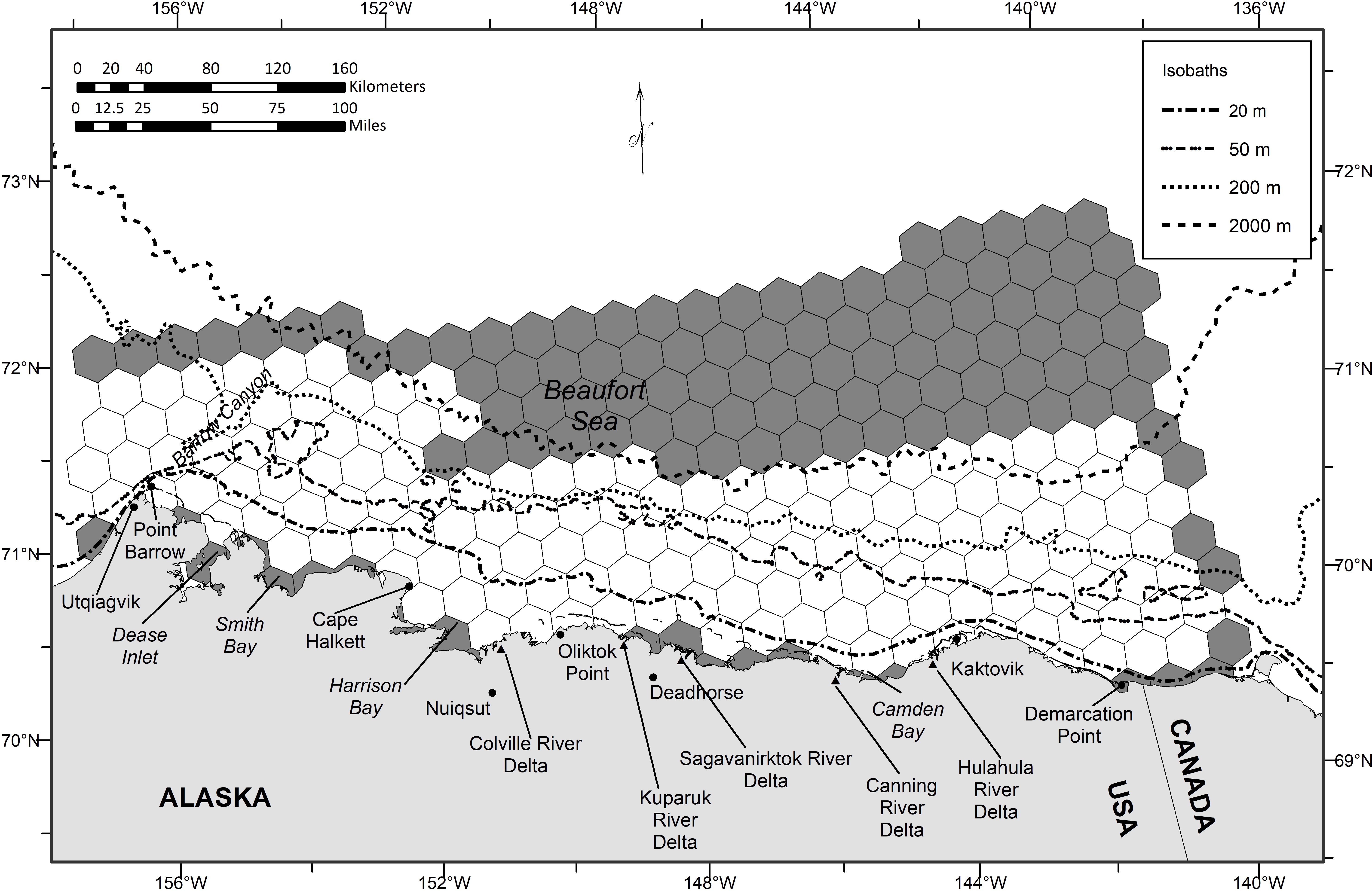
Figure 1 Study area in the western Beaufort Sea. Unshaded hexagonal cells represent those that the spatial optimization models could select to be delineated as Biologically Important Areas.

2.2 Aerial survey methods

A brief overview of the field methods is provided here. See Clarke et al. (2019) and Clarke et al. (2020) for detailed information.

Line-transect aerial surveys were flown in the western Beaufort Sea during summer (July-August) 2012-2019 and autumn (September-October) 2000-2019 as part of the Aerial Surveys of Arctic Marine Mammals (ASAMM) project. ASAMM was funded and co-managed by the Bureau of Ocean Energy Management and conducted and co-managed by NOAA. Systematic transects were placed 19 km apart, based on a grid with a randomly selected start point. Transects were approximately 80-175 km long, oriented perpendicular to the coastline, to cut across isobaths, from shore to beyond the 2,000-m isobath.

Surveys were flown in de Havilland Twin Otters and Turbo Commanders, twin turbine aircraft with bubble windows on the left and right sides, allowing unobstructed views from the horizon to the transect directly beneath the aircraft. The aircraft were based out of Utqiaġvik and Deadhorse, Alaska. Surveys were flown 305-460 m above the sea surface, at 213 km/hr survey speed.

Each survey team comprised two primary observers and one dedicated data recorder. The data recorder input sighting data into a laptop computer, connected to a global positioning system, running specialized, menu-driven ASAMM Survey software. Time and position data (latitude, longitude, altitude) were automatically recorded every 30 seconds (in time) or whenever a manual data entry was recorded. Environmental and viewing conditions were recorded every 5 minutes (in time) or whenever conditions changed. Primary observers scanned the seascape with naked eye, using binoculars only to check potential targets or to get a magnified view of a confirmed target. Declination angles from the horizon to each sighting were measured using handheld Suunto clinometers once the sighting was abeam. A “sighting” was defined as all animals of the same species within 5 body lengths of each other. Once the declination angle was recorded, most sightings of large cetaceans (anything larger than a beluga, Delphinapterus leucas) were circled to determine a final group size estimate, confirm species identification, look for calves, and determine behavior. Both initial and final group size estimates were recorded in the database; if group size could not be determined with certainty, high and low estimates could also be recorded. The database distinguished between calves initially detected from the trackline and calves that were only detected during circling. Circling did not commence in special circumstances, such as restrictions due to weather, fuel, time of day, or duty hours, or in the vicinity of sensitive wildlife or subsistence hunting activities. Sightings that could not be positively identified to species were recorded at the taxonomic level to which they could be identified (e.g., “unidentified cetacean”).

Bowhead whale demographic classification was based on morphology and behavior. Most bowhead whale calves are born in spring and early summer (April to June) (Tarpley et al., 2021), although recently-born calves have been reported as late as August (Koski et al., 1993). Small bowhead whales that have a streamlined appearance, have small heads compared to their body lengths, are light gray in color, or are in close association with adult bowhead whales are likely to be calves born that year. Calves observed without an adult nearby are likely associated with a cow that is completely submerged, especially when feeding. In autumn, calves are more rotund than calves observed in summer. If an individual’s age class was uncertain, the animal was not designated as a calf in the ASAMM database.

The complete list of cetacean behaviors and associated definitions is provided in Clarke et al. (2020). Feeding behavior for bowhead whales was defined as the “[a]nimal(s) diving repeatedly in a fixed area, sometimes with mud streaming from the mouth and/or defecation observed upon surfacing; synchronous diving and surfacing or echelon formations at the surface, with swaths of clearer water behind the whale(s), or surface swimming with mouth agape”. Milling behavior was defined as “[t]wo or more animals moving slowly at the surface with varying headings, in close proximity (within 100 m) to, but not obviously interacting with, other animals”. Bowhead whales feed on the seafloor, in the middle of the water column, or at the surface of the water. Milling behavior could be indicative of subsurface feeding. Behavior could also be recorded as “swim” or “unknown” or left blank.

Data collected during the four survey modes transect, circling from transect, Cetacean Aggregation Protocols (CAPs) passing, and CAPs circling (Clarke et al., 2019) were used in the optimization model introduced below in Section 2.3.1. During all four of these survey modes, observers were actively surveying and all marine mammal sightings and effort data were recorded. Transect effort refers to systematic survey effort along a prescribed transect line. Circling from transect occured when the aircraft diverted from flat and level flight on transect to circle a localized area to investigate a sighting or potential sighting. Standard line-transect survey protocols were followed until large whale encounter rates exceeded the observers’ ability to accurately record location and declination angle to each sighting. In areas with extremely high densities of large whales, CAPs was used, wherein the survey team flew through the high-density aggregation in passing mode (without circling) to collect accurate encounter rate data, and then flew back through the aggregation in closing (CAPs circling) mode to collect information on group size, number of calves, and behavior (Clarke et al., 2019; Clarke et al., 2020).

2.3 Analytical methods

The study area was divided into a lattice composed of hexagonal cells with 25-km resolution (Figure 1). This analytical resolution was chosen based on the resolution of the data, as transects are spaced approximately 19 km apart, and on current understanding of the scale of the ecological mechanisms that drive spatiotemporal variability in bowhead whale density in the western Beaufort Sea (Ferguson et al., 2021).

Only a subset of the entire ASAMM western Beaufort Sea survey region was included in the analyses. The subset was defined as all cells with at least one sighting of a feeding or milling bowhead whale or a bowhead whale calf any time from July through October 2000-2019. Because the marine environment is dynamic and we wanted to examine whether it was optimal to include cells without sightings to support spatially cohesive networks, cells without any bowhead whale sightings that were surrounded by cells with bowhead whale sightings were also included in the analyses.

For transect and CAPs passing survey modes, the total kilometers surveyed, observed encounter rate (number of whales per kilometer) of feeding or milling (equivalently denoted by feeding/milling) bowhead whales, and observed encounter rate of bowhead whale calves were summarized for each cell-month-year combination. The number of whales on transect used to compute encounter rate corresponded to the final group size associated with records of feeding and milling whales or the total number of calves, including calves sighted during circling. The number of whales on CAPs was computed following the methods detailed in Appendix A of Ferguson (2020). Feeding/milling whale models were based on ASAMM data from 2000 to 2019. Calf models were limited to data from 2012 to 2019, when the western Beaufort Sea study area was surveyed consistently from July through October.

2.3.1 Delineating BIAs using spatial optimization methods

Our first objective was to maximize the number of feeding and milling bowhead whales or calves in selected areas, contingent upon spatial contiguity and total area constraints. Spatial contiguity may be desirable for both practical and ecological reasons. It may be simpler to monitor, enforce, and adhere to fewer contiguous management units than numerous dispersed islands of management units. Additionally, spatial contiguity is often associated with ecological integrity (e.g., IUCN, 2016) because it minimizes edge effects and facilitates movement and dispersal (Williams et al., 2005). Our optimization model can be formulated for any maximum total area, allowing the analyst to quantify the tradeoffs associated with alternative values.

Linear binary integer programming problems seek to maximize (or minimize) a linear objective function, $a^{\prime }x={\sum }_{i=1}^n{a}_i{x}_i$, over all n-dimensional vectors x = (x₁, …, x_n), where x_i may take the value of 0 or 1, and the maximization is subject to a set of linear inequality constraints (Bertsimas and Tsitsiklis, 1997). The vector a= (a₁, …, a_n) provides the value associated with each of the n decision variables, x₁, …, x_n. This linear binary integer programming problem can be expressed using vectors a, b, x, and matrix C as

maximize a’x

subject to Cx ≥ b

x ≥ 0

x ∈ {0,1}.

Inequalities such as Cx ≥ b are interpreted component-wise; that is, for every i, the ith component of the vector Cx, which is c’_ix, is greater than or equal to the ith component b_i of the vector b. A vector x satisfying all the constraints is called a feasible solution. A feasible solution x* that maximizes the objective function (that is, a’x* ≥ a’x, for all feasible x) is called an optimal feasible solution or, equivalently, an optimal solution. The value of a’x* is then called the optimal value. Depending on the problem, there may exist only one, multiple, or no optimal solutions. A key feature of this analysis is that linear binary integer programming searches for a global optimal solution. This contrasts with methods such as simulated annealing (e.g., Airamé et al., 2003; Leslie et al., 2003), which seek only an approximation of the optimum.

More specifically, the methods of Tóth et al. (2009) formed the basis of the analysis. The following is a formal, mathematical description of our optimization model formulation. We start with the definitions of variables, model parameters, and other mathematical objects (e.g., sets) that we use in the model:

Variables (both binary):

x_i = 1 if cell i is selected, 0 otherwise;

y_j = 1 if cluster j is selected, 0 otherwise.

Parameters:

d_i = relative density (encounter rate) of feeding/milling whales or calves in cell i, defined as the number of whales observed per square kilometer surveyed, assuming an effective strip width of 1 km;

a_i = area of cell i;

Z = proportion of occupied cells enclosed by BIA boundaries, where a cell is considered to be “occupied” if it had at least one sighting of feeding/milling bowhead whales or calves (as appropriate, depending on BIA type) during aerial surveys conducted in the specified month, pooled across all years;

δ = minimum d_i>0;

occ.cells = number of occupied cells;

Sets:

I = the set of all cells

P_i = the set of clusters that contain cell i;

C_j = the set of cells that comprise cluster j;

|C_j| = the number of cells that comprise cluster j (the cardinality of cluster j);

C = the set of all possible clusters.

Our integer programming model formulation is as follows:

$\begin{array}{ll}Max{\sum }_i{d}_i{a}_i{x}_i& \text{[1]}\end{array}$

Subject to:

$\begin{array}{ll}\frac{1}{occ.cells}\sum _{}\underset{i}{}{x}_i\le Z\text{ for each }i\in I& \text{[2]}\end{array}$

$\begin{array}{ll}{x}_i\le \sum _{}\underset{j\in P_i}{}{y}_j\text{ for each }i\in I& \text{[3]}\end{array}$

$\begin{array}{ll}\sum _{}\underset{i\in C_j}{}{x}_i\ge \left|C_j\right|y_j\text{ for each }{C}_j\in C& \text{[4]}\end{array}$

$\begin{array}{ll}\sum _{}\underset{i\in C_j}{}{x}_i-\left|C_j\right|+1 \le y_j\text{ for each }{C}_j\in C& \text{[5]}\end{array}$

$\begin{array}{ll}\frac{1}{\delta }\sum _{}\underset{i\in C_j}{}{d}_i{x}_i\ge y_j\text{ for each }{C}_j\in C& \text{[6]}\end{array}$

$\begin{array}{ll}{x}_i\in \left\{0,1\right\}& \text{[7]}\end{array}$

$\begin{array}{ll}{y}_j\in \left\{0,1\right\}& \text{[8]}\end{array}$

The objective function [1] maximizes the total number of bowhead whales detected during aerial surveys within the areas enclosed by the selected BIAs.

Constraint [2] limits the maximum total area selected for BIAs in terms of the proportion (Z) of occupied cells rather than a proportion of the study area. Our rationale for defining the area constraint this way is that the cells where bowhead whales are known to engage in a particular activity are the ecological features of interest, whereas study area boundaries may be somewhat arbitrary.

Constraint [3] ensures that any cell i can be selected to be part of a BIA if and only if it is part of at least one feasible cluster of cells that is selected as a BIA.

Inequality [4] states that variable y_j corresponding to cluster j may be set to 1 if every single cell in that cluster is selected. Conversely, if y_j is set to one, this forces all cells in C_j to be included in the BIA. That is, if y_j=1, then the right-hand side (RHS) of this constraint will equal the cardinality of set C_j, which in turn is the number of cells in cluster j. Because the left-hand-side (LHS) simply sums the number of cells in cluster j that are selected, then y_j=1 will force all of them to be selected. If on the other hand y_j=0, then, per Inequality [4], the number of cells in cluster j that can be selected must be strictly less than the cardinality of C_j (or, equivalently the number of cells in cluster j). This enforces that y_j can turn on if and only if all of its elements (its cells) are selected.

If x_i=1, then Inequality [3] forces at least one of the clusters that contain cell i (set P_i) to take the value of 1. For each cluster in set P_i that ends up with y_j=1, all cells in that C_j will also be forced to take the value of 1 per Inequality [4]. If on the other hand x_i=0, then Inequality [3] becomes inactive (i.e., the RHS can take any integer value between 0 and the cardinality of P_i). However, if x_i=0, Inequality [4] is activated for each cluster in P_i. Namely, Inequality [4] will force all y_j’s representing clusters in P_i to be 0 because they cannot possibly be protected if not all cells including cell i are selected.

Inequality [5] works in concert with [4]. Not only does the former allow but it forces y_j=1 if all cells in C_j are selected. To see this, consider a cluster that comprises four cells (in other words, the cardinality of this cluster is 4, | C_j | = 4). If all cells in this cluster are selected, then the sum on the LHS will equal 4. This makes the value of the LHS of the inequality [5] equal to 1, which in turn forces y_j to be 1. Otherwise, the inequality [5] would not hold as 1 is not less than or equal to 0.

Lastly, Inequality [6] ensures that only clusters with at least one observed feeding/milling bowhead whale or bowhead whale calf can be a BIA. Without [6], the model could allow empty (unoccupied) clusters into the solution if there were space to add cells before reaching the area threshold (Z) after all cells with applicable bowhead whale observations had been included in the solution.

A single cell may be found in more than one cluster in the optimal solution; that is, clusters in the optimal solution may overlap. The objective function [1] and maximum area threshold [2] operate at the cell level. Therefore, if a cell enters the optimal solution because it is a member of overlapping clusters in the solution, the number of whales in that cell will be counted only once towards the value of the objective function, and the area of that cell will be counted only once against the maximum area threshold.

Our recursive cluster enumeration algorithm proceeded as follows. We use the notation:= to mean “defined to be equal to”.

Initialization: Set Index x:= 0, Index j:= 0. For each Cell i∋I generate a list of cells A_i that are adjacent to Cell i: A_i ∀i∋I. Cells were considered adjacent when they shared a common boundary.

Step 1: Is set I empty (I = {Ø})? If yes, Terminate. Otherwise, set Index j:= j + 1, create a new empty Cluster j set area of Cluster j equal to 0 (a_j:= 0) and go to Step 2.

Step 2: Select any Cell i∋I and remove it from Set I (I:= \{i}). Add Cell i to Cluster j (j∶=j∪^​i) and add the area of Cell i (a_i) to the area of Cluster j (a_j∶=a_j+1 ) Set x: = i.

Step 3: Does Cell x not have any adjacent cells (A_x = {Ø})? If yes, go to Step 1. Otherwise, go to Step 4.

Step 4: Select any Cell c∋A_x that is not already included in Cluster j. Add Cell c to Cluster j (j∶=j∪^​c, a_j∶=a_j+1) Go to Step 5.

Step 5: Does the area of Cluster j equal the minimum cluster size a_min (a_j = a_min)? If yes, save Cluster j as feasible cluster and go to Step 1. Otherwise, set x:= c and then go to Step 3.

Post-processing: Remove identical clusters (combinations of cells) and leave only one copy of each.

This model was formulated for different scenarios, where a scenario was defined by the BIA type (feeding/milling or calf), month (July, August, September, October), minimum cluster size (1, 2, 3, 4, 5), and area threshold (Z = 0.1 to 1.2, by 0.1). Based on our knowledge of bowhead whale distribution in the study area and the spatial range of relevant biophysical processes that shape seasonal spatiotemporal variability in Arctic marine environments (Moore et al., 2018), we set the upper limit for minimum cluster size to 5 cells. Z was allowed to range up to 1.2 (delineation encompassing 120% of occupied cells) to allow the models with minimum cluster size greater than 1 to incorporate all occupied cells; the minimum cluster size restriction sometimes required empty cells to be incorporated into the solution in order to allow an adjacent occupied cell to enter the solution. Data for each model were pooled across years.

We solved our optimization model with a commercial integer programming solver and mapped the BIA selections that resulted from these model runs. For each BIA type and month, a single scenario (contiguity threshold and area threshold) was selected based on visual inspection as the basis for the inter-annual variability analysis detailed in Section 2.3.2 below. Scenario selection was based on the judgment of experts with 28 (JTC), 13 (MCF), and 12 (AAB) years of experience analyzing ASAMM data or conducting ASAMM surveys in the western Beaufort Sea. Expert elicitation is a common tool used in conservation science and natural resource management in general (e.g., Danovaro et al., 2020; Lettrich et al., 2020) and spatial planning in particular (e.g., Thomson et al., 2020). The rationale for selecting each scenario was based on direct knowledge of the inherent patchiness in bowhead whale density and ecological drivers of spatiotemporal variability in bowhead whale density in the western Beaufort Sea.

The spatial optimization analyses were conducted in R version 3.62 (R Core Team, 2019) and CPLEX Studio version 12.9.0.0. The following R packages were used: sp (Pebesma and Bivand, 2005; Bivand et al., 2013), maptools (Bivand and Lewin-Koh, 2019), rgeos (Bivand and Rundel, 2019), rgdal (Bivand et al., 2019), ggplot2 (Wickham, 2016), and dichromat (Lumley, 2013). The optimization models were solved in CPLEX, using default parameters. We instructed CPLEX to abort either if the default 0.01% optimality gap or the 1 hour of runtime limit was reached. All analyses were conducted on a PC laptop computer with an Intel(R) Core(TM) i7-8650U CPU @ 1.90GHz 2.11 GHz processor.

2.3.2 Quantifying BIA inter-annual variability

Classifying areas according to their temporal characteristics can provide insight into the methods needed to monitor the ecosystem and anthropogenic activities in the area, and to minimize or mitigate risks to the ecosystem from human activities. For example, the Convention on Biological Diversity created a classification scheme to classify EBSAs into four categories (Johnson et al., 2018): static features, groups of features, ephemeral features, and dynamic features. However, there is no clear way to rank the ecological significance of a feature based on these temporal characteristics, so we did not incorporate them into our optimization model. Because most BIAs were defined by month and the remainder were defined by season, we focus the following investigation of temporal variation on inter-annual variability.

Specifically, once we solved the monthly bowhead whale calf and feeding spatial optimization models for each combination of maximum area threshold and cluster size, we used expert judgement to select a single characteristic scenario (i.e., maximum area threshold and minimum cluster size) for each month and BIA type (calves and feeding). Then, for each selected scenario, we used statistical analyses to quantify inter-annual variability within each of the BIA units identified by the optimization model. We define inter-annual variability as the differences across years in bowhead whale occurrence or density during a given month in a particular BIA unit. The BIA unit is defined as one or more cells sharing at least one boundary with a neighboring cell that was delineated in the selected scenarios described above. The two types of metrics used to quantify inter-annual variability are: (1) empirical statistics from observed bowhead whale sightings and survey effort; and (2) the standard deviation of the random effect of year from generalized linear mixed models (GLMMs).

The empirical statistical analysis follows the methods that Sigler et al. (2017) used to identify persistent prey hotspots. For each combination of BIA type, month, and spatial resolution, we calculated the number of years in which at least one bowhead whale (feeding/milling or calf, as appropriate) was sighted (Y_bowhead; “bowhead whale years”), the number of survey years in which surveys were conducted (Y_survey; “survey years”), and the ratio of these two values, which we refer to as the proportion of bowhead whale years (p_bowhead):

$\begin{array}{ll}{\text{p}}_{\text{bowhead}}{\text{ = Y}}_{\text{bowhead}}{\text{/Y}}_{\text{survey.}}& \text{[9]}\end{array}$

The second analysis of inter-annual variability was applied independently to each BIA and involved a simple Poisson GLMM with random effects for year (y ϵ {2000,…, 2019} for the feeding/milling BIAs; y ϵ {2012,…,2019} for the calf BIAs):

$\begin{array}{ll}lo{g}_e[E(w_{i,y}|{\gamma }_{i,y})]={\beta }_i+{\gamma }_{i,y}+lo{g}_e(k{m}_{i,y})& \text{[10]}\end{array}$

This formulation uses a natural logarithmic link function to relate the expected number of bowhead whales (w) in BIA i and year y to a linear predictor comprised of three terms: an overall mean value (the fixed intercept) β_i; a random effect for year, γ_i,y, which represents the deviation around the mean that can be attributed to inter-annual variability; and an offset for the natural logarithm of the number of kilometers flown on transect and CAPs passing in area i and year y. It is assumed that the random effect for year comes from a normal distribution with zero mean and variance ${\sigma }_{i,y}^2$

$\begin{array}{ll}{\gamma }_{i,y}~N(0,{\sigma }_{i,y}^2)& \text{[11]}\end{array}$

Only years with non-zero survey effort were included in each GLMM. Because the number of whales on CAPs is not restricted to integer values (Ferguson, 2020), w_i was rounded to the nearest integer for parameterizing the GLMMs. (Non-integer w_i was only an issue for one BIA in the September calf analysis and one BIA in the October calf analysis.) Applying the inverse link function, exp(·) to [10] gives:

$\begin{array}{ll}E(w_{i,y}|{\gamma }_{i,y})=exp[{\beta }_i+{\gamma }_{i,y}+lo{g}_e(k{m}_{i,y})]& \text{[12]}\end{array}$

In [12] it is clear that the expected number of whales is conditioned on the random effect for year, as is standard in GLMMs. The statistical distribution for this model can be represented as:

$\begin{array}{ll}{w}_{i,y}|{\gamma }_{i,y}~Pois\left\{exp[{\beta }_i+{\gamma }_{i,y}+lo{g}_e(k{m}_{i,y})]\right\}& \text{[13]}\end{array}$

The investigation into inter-annual variability was conducted in R version 3.62 (R Core Team, 2019), using package lme4 (Bates et al., 2015) in addition to those packages detailed above.

3 Results

We will first present the results of our aerial surveys as this information was critical to formulating and parameterizing our optimal BIA selection models whose solutions will be given next, along with a description of the computational cost of running the models. Lastly, we will describe the results of our inter-annual variability analyses conducted based on these solutions to the optimization models.

3.1 Survey effort and sighting summaries

The distribution and density of line-transect survey effort and bowhead whale sightings (by activity state) differed by month and year. We present a summary of the results here and provide supplementary graphics in Appendix S1.

We begin with a summary of transect and CAPs survey effort and bowhead whale sightings in the study area from 2000 to 2019, the years used in the analysis of feeding and milling whales. September had the most survey effort overall (134,819 km) and the highest median effort per cell (916 km); July had the least overall (40,749 km) and the lowest median effort per cell (253 km) (Table 1). Survey effort per cell and month (all years pooled) ranged from a minimum of 22 km per cell in October to a maximum of 1,637 km in September (Table 1, Appendix S1: Figure S1). During each month, survey effort covered the longitudinal range of the study area, extending to waters deeper than 2,000 m, although it was mostly concentrated in waters from 0 to 200 m (Appendix S1: Figure S1). Summer (July and August) survey effort was limited from 2000 to 2011, whereas autumn (September and October) survey effort was more consistent across all years (Appendix S1: Figure S2). Survey effort per cell by month and year ranged from 0 km in some months and years, to a maximum of 258 km in September 2015 (Appendix S1: Figure S2). September generally had the most survey effort due to a combination of factors, including weather and timing of the bowhead whale migration.

TABLE 1

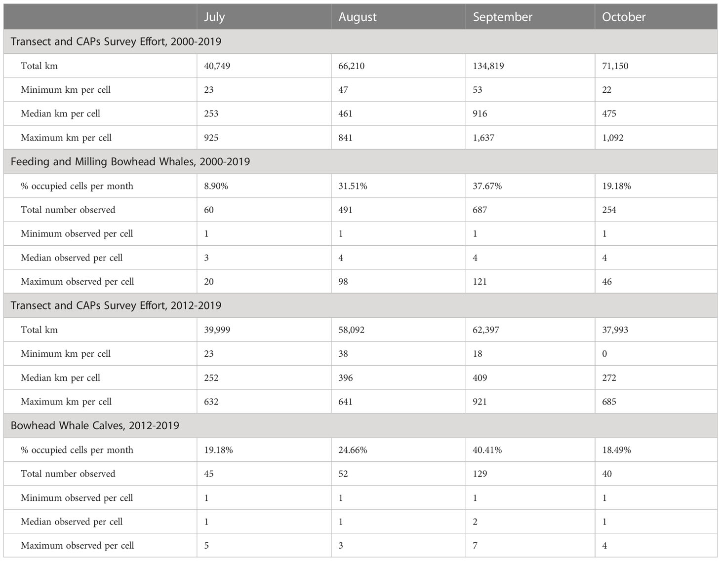
Table 1 Summary of survey effort and bowhead whale sightings from aerial surveys in the western Beaufort Sea study area during transect and Cetacean Aggregation Protocols (CAPs) survey modes from 2000 to 2019 (feeding and milling analysis years), and from 2012 to 2019 (calf analysis years).

From 2000 to 2019, September had the most feeding and milling bowhead whales detected overall (687 whales) and per cell (121 whales), and the greatest percentage of occupied cells (37.67%) (Table 1; Appendix S1: Figure S3). There was considerable inter-annual variability in the number of feeding and milling bowhead whales per cell by month, with no observations during some months in some years and the most observations per cell during August 2016 and September 2017 (Appendix S1: Figure S4). August was the month with the highest encounter rates per cell (Appendix S1: Figure S5). The depth distribution of feeding and milling whales was farthest offshore in July, closer to shore in August, and closest to shore in September and October (Appendix S1: Figure S5). Additionally, the distribution of feeding and milling activity progressed westward from July through October (Appendix S1: Figure S5). BIAs for bowhead whale feeding that were delineated in the original effort (Clarke et al., 2015) are shown in Appendix S1: Figures S3, S5.

The calf analyses were limited to data from 2012 to 2019. Approximately 74% (433 of 582 calves) of the bowhead whale calves recorded throughout the ASAMM study area during this period were initially detected during circling effort. September was the month with the most survey effort (62,397 km) and July had the least (39,999 km) (Table 1). Combined transect and CAPs survey effort per cell and month (2012-2019 pooled) ranged from 0 km to 921 km (Table 1, Appendix S1: Figure S6), and show patterns with respect to depth and longitude consistent with those for the longer time series beginning in 2000 (Appendix S1: Figure S1).

September had the most bowhead whale calves detected per cell (7 calves), the greatest total number of calves throughout the study area (129 calves), the broadest distribution of calves, and the highest percentage of cells with calves (Table 1; Appendix S1: Figures S7, S8), although the highest calf encounter rate occurred in August (Appendix S1: Figure S9). Calves were observed in all months except August 2018, although inter-annual variability in calf sightings per cell is evident (Appendix S1: Figure S8). Calves were encountered farther offshore and in the eastern half of the study area during July, and their distribution moved closer to shore and westward as the survey season progressed (Appendix S1: Figure S9). The BIAs for bowhead whale reproduction that were delineated in the original effort are shown in Appendix S1: Figures S7, S9.

3.2 BIAs delineated using spatial optimization methods

3.2.1 Computational costs

Running the cluster enumeration algorithm for both BIA types (feeding and calves), all four months, all twelve maximum area constraints, and minimum cluster sizes 2, 3, 4, and 5 (2*4*12*4 = 384 total models) required approximately 4.5 hours of computing time. The sum total time to find the optimal solutions for these 384 scenarios was approximately 19.5 hours. For these 384 scenarios, the optimality gap was the binding constraint in all cases except for 13 scenarios that had a minimum cluster size of 5 and that reached the maximum run-time limit of 1 hour. It took only two minutes to find the optimal solutions for all of the scenarios with minimum cluster size of 1 (2 BIA types * 4 months * 12 max area thresholds = 96 total scenarios).

3.2.2 Model results

The number of possible clusters in the study area increased nonlinearly with increasing minimum cluster size. The study area comprised a total of 146 cells, including 331 pairs of cells sharing a common border, 892 possible 3-cell clusters, 2,269 possible 4-cell clusters, and 5,308 possible 5-cell clusters.

The optimization models resulted in three consistent patterns with respect to minimum cluster size and maximum area threshold for both BIA types and all months. First, cells with the highest density were selected when contiguity or maximum area thresholds were small (Appendix S2). Second, for a given area threshold, the number of feeding/milling whales or calves inside BIAs was inversely proportional to cluster size. This result occurred because a smaller minimum cluster size provided the model with more freedom to select cells with the highest whale densities (Figures 2, 3; Appendix S2). As minimum cluster size increased, the model was forced to select cells with zero observed whales to add clusters containing relatively high densities of whales (Figures 2, 3; Appendix S2). Third, the number of feeding/milling whales or calves inside BIA boundaries initially increased rapidly as the area threshold increased, but eventually approached an asymptote near Z ≥ 1.0 (Figures 2, 3). This result reflects the models’ preference for selecting the cells with the lowest density last. Scenarios selected for further consideration in the analysis of inter-annual variability used minimum cluster size of either 2 or 3, and area threshold of Z = 0.5 or 0.7 (Table 2).

FIGURE 2

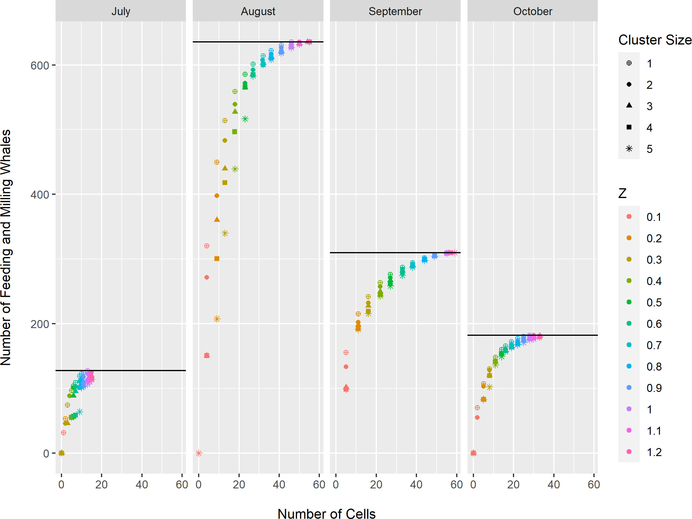
Figure 2 Estimated number of feeding/milling bowhead whales (Eqn. 1) enclosed by Biologically Important Areas for spatial optimization models constructed for each month (July-October), minimum contiguity threshold (cluster size 1-5), and maximum occupied area threshold (Z = 0.1, 0.2, 0.3, 0.4, 0.5, 0.6, 0.7, 0.8, 0.9, 1.0, 1.1, 1.2). The black horizontal line in each column represents the total number of observed feeding/milling bowhead whales for that month.

FIGURE 3

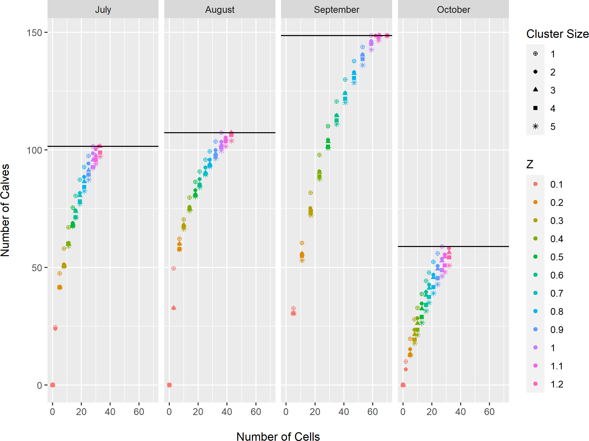
Figure 3 Estimated number of bowhead whale calves (Eqn. 1) enclosed by Biologically Important Areas for spatial optimization models constructed for each month (July-October), minimum contiguity threshold (cluster size 1-5), and maximum occupied area threshold (Z = 0.1, 0.2, 0.3, 0.4, 0.5, 0.6, 0.7, 0.8, 0.9, 1.0, 1.1, 1.2). The black horizontal line in each column represents the total number of observed bowhead whale calves for that month.

TABLE 2

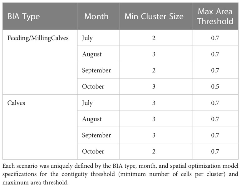
Table 2 Spatial optimization model scenarios selected for the analysis of inter-annual variability in bowhead whale feeding/milling and calf Biologically Important Areas (BIAs).

Results from the September feeding/milling and calf models are summarized here. Figures for both BIA types and all months, cluster sizes, and area thresholds are presented in Appendix S2.

The selected scenario for September feeding/milling bowhead whales was the 2-cell cluster optimization model with maximum area threshold of Z = 0.7. At the lowest area threshold of 0.1, the optimization model for feeding/milling bowhead whales in September selected high density cells located in the nearshore “krill trap area” east of Point Barrow and in coastal waters between Prudhoe and Camden bays, which are influenced by upwelling and freshwater discharge from rivers (Appendix S2: Figure S12). As the area threshold increased, cells with lower whale densities were incorporated into the solution, first incorporating cells off Cape Halkett and east of Kaktovik, and eventually adding all cells with observations of feeding/milling bowhead whales.

The selected scenario for September bowhead whale calves was the 3-cell cluster optimization model with maximum area threshold of Z = 0.7. The September bowhead whale calf optimization model selected cells with high calf densities in the vicinity of Camden Bay under the lowest area threshold (Z = 0.1) (Appendix S2: Figure S33). As the maximum area threshold was relaxed, solutions began to incorporate more cells on the inner continental shelf, stretching eastward to the US-Canada border, before encompassing the lower density cells in the central and western portions of the study area. The relatively low density cells near Barrow Canyon were among the last to be added to the solution.

The September calf BIAs provide an instructive example of the potential effects of cluster size on optimal delineation of BIAs. In the selected scenario (minimum cluster size 3, maximum area threshold Z = 0.7), there were no calf BIAs delineated in the nearshore cells between Point Barrow and Smith Bay. However, two nearshore cells north and west of Smith Bay were included among the BIAs for the scenario with minimum cluster size of 2 cells and maximum area threshold Z = 0.7 (Appendix S2: Figure S32D).

3.3 Inter-annual variability in BIAs

Results from the September analyses of inter-annual variability of feeding/milling and calf BIAs are summarized here. Analogous figures for the remaining selected scenarios are provided in Appendix S3.

The six BIAs delineated for feeding and milling bowhead whales in the selected scenario for September were (from west to east) krill trap, offshore Harrison Bay, Harrison Bay to Deadhorse, Camden Bay, east of Kaktovik, and Demarcation Point (Figure 4A and Appendix 3: Figure S3). The number of bowhead whale years ranged from 2 to 12 years (Figure 4B and Appendix 3: Figure S3). The number of survey years ranged from 18 to 20 years (Figure 4B and Appendix 3: Figure S3). The proportion of bowhead whale years, p_bowhead, ranged from 0.11 to 0.60 (Figure 4B and Appendix 3: Figure S3). BIAs ranked from highest to lowest GLMM fixed intercept (β_i) were: 1) krill trap; 2) Harrison Bay to Deadhorse; 3) offshore Harrison Bay; 4) east of Kaktovik; 5) Demarcation Point; and 6) Camden Bay (Figure 4B and Appendix 3: Figure S3). BIA ranks based on p_bowhead were similar, but not identical, to the β_i ranks (Figure 4B and Appendix 3: Figure S3). By contrast, BIA ranks based on the standard deviation of the random effect for year (σ_i,y) were the reverse of the β_i ranks (Figure 4B and Appendix 3: Figure S3). These results suggest that the highest average density (largest β_i) bowhead whale feeding and milling areas in the study area are also relatively stable, both in terms of occurrence (largest p_bowhead) and density (smallest σ_i,y) from year to year.

FIGURE 4

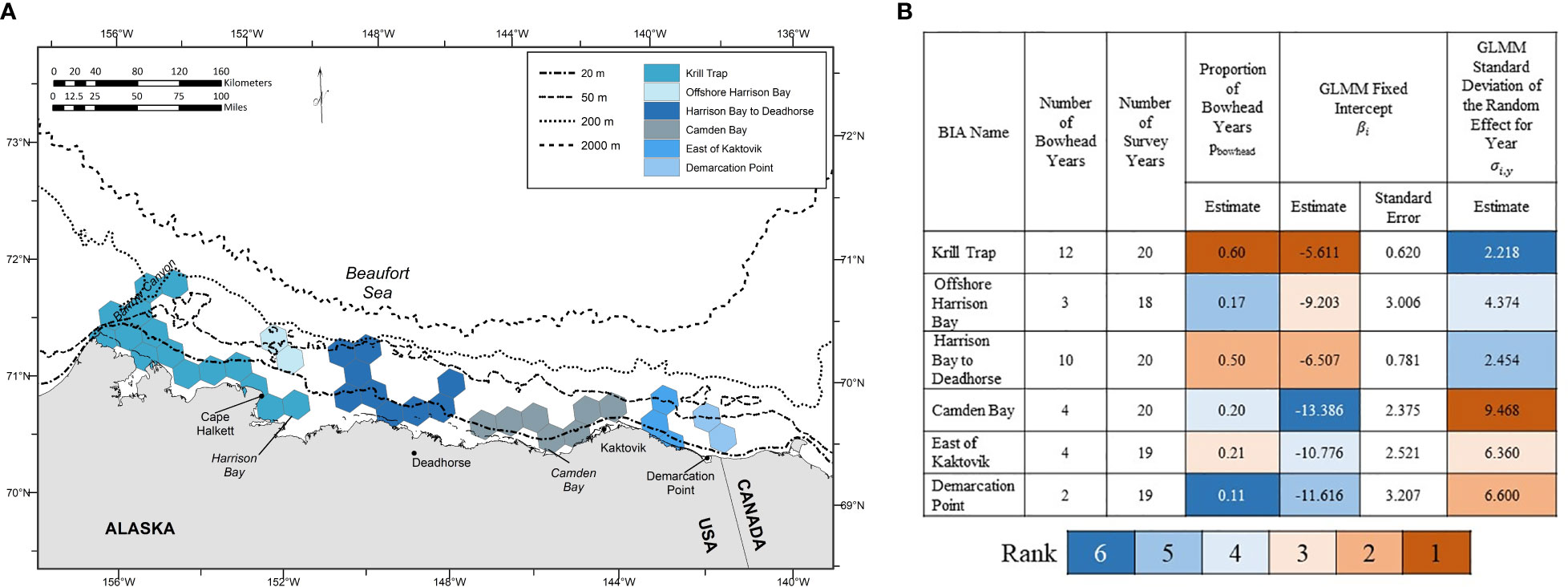
Figure 4 Results of the inter-annual variability analysis for each of the six Biologically Important Areas (BIAs) identified in the selected scenario for feeding/milling bowhead whales in September. (A) Geographic location. (B) Summary statistics and GLMM parameter estimates. Parameter estimates are color-coded based on their associated rank, from high (rank 1) to low (rank 6).

The five BIAs delineated for bowhead whale calves in the selected scenario for September were (from west to east) Barrow Canyon, Cape Halkett, offshore Harrison Bay, central Alaskan Beaufort, and eastern Alaskan Beaufort (Figure 5A and Appendix S3: Figure S7). The number of bowhead whale years ranged from 3 to 8 yrs (Figure 5B and Appendix S3: Figure S7). Every BIA had 8 survey years (Figure 5B and Appendix S3: Figure S7). Values of p_bowhead ranged from 0.4 to 1.0 (Figure 5B and Appendix S3: Figure S7). Although σ_i,y for Cape Halkett and offshore Harrison Bay were estimated to be zero (the GLMMs were singular; Figure 5B), this result may be due to the small sample size. The relationships among the different inter-annual variability metrics for bowhead whale calves were more complicated than those for feeding and milling bowhead whales. For example, the eastern Alaskan Beaufort BIA had the highest of both p_bowhead and σ_i,y, but ranked third in β_i Figure 5B). In other words, calves are consistently found in the eastern Alaskan Beaufort, but inter-annual variability in density is relatively large. Barrow Canyon ranked 2^nd for σ_i,y (relatively high inter-annual variability in calf density), 3.5^th for p_bowhead, and last for β_i (relatively low average calf density).

FIGURE 5

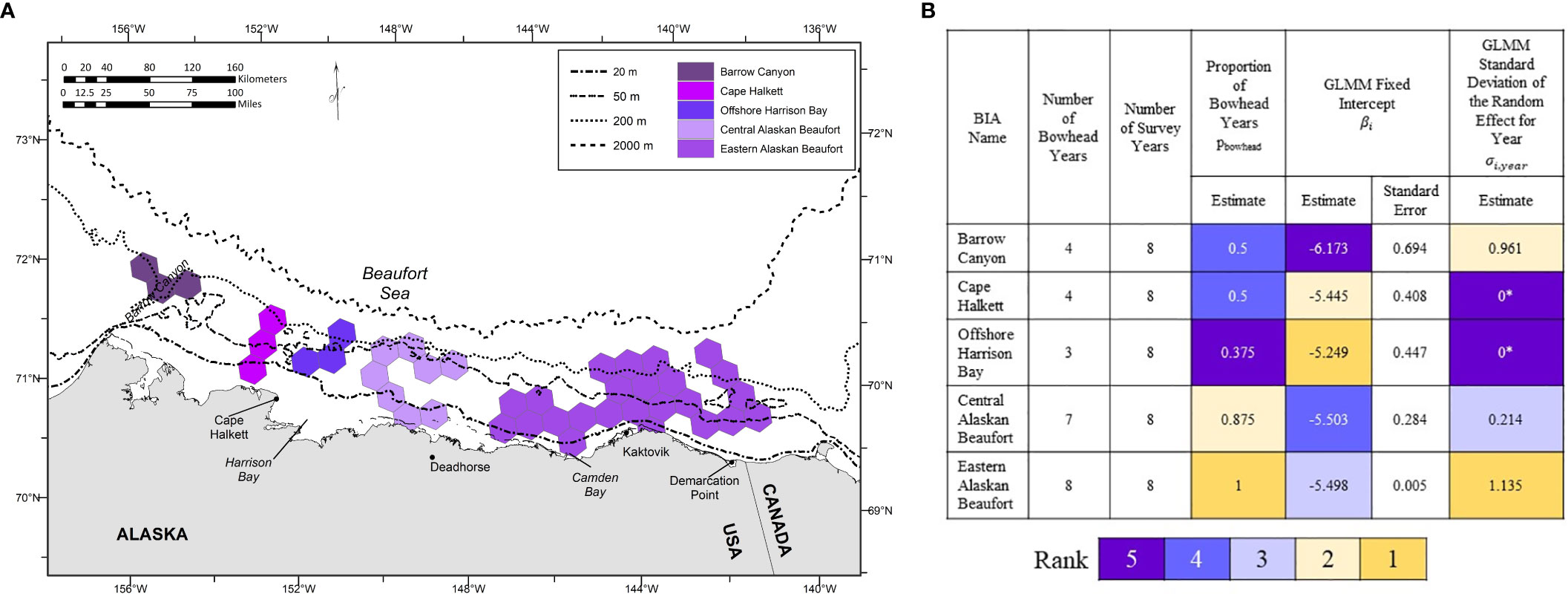
Figure 5 Results of the inter-annual variability analysis for each of the five Biologically Important Areas (BIAs) identified in the selected scenario for bowhead whale calves in September. (A) Geographic location. (B) Summary statistics and GLMM parameter estimates. Parameter estimates are color-coded based on their associated rank, from high (rank 1) to low (rank 5). ^*Singular model; σ_i,y estimated to be zero.

4 Discussion

We provide an objective and reproducible analytical framework for optimally delineating areas that are biologically important for cetaceans that explicitly addresses size and spatial contiguity. We also provide methods for characterizing the temporal variability in cetacean occurrence or density in a given area. We hope that by explicitly incorporating spatial and temporal characteristics of the species into the BIA evaluation process, we have ultimately produced an effective tool that can be incorporated with other relevant information (e.g., project objectives, ecological stressors, costs, acceptable risk, legal constraints) into conservation and management decision-making processes. Additionally, we have identified areas that have real ecological value to bowhead whales. This, in turn, will help focus localized, collaborative investigations to better understand the ecological mechanisms driving the spatiotemporal variability in bowhead whale density in the western Beaufort Sea.

Ecological mechanisms known to affect bowhead whale prey density and availability in the September feeding/milling BIAs identified here include a combination of local and remote drivers (Ferguson et al., 2021). Local winds may generate upwelling and affect the pathway of currents, mechanisms that establish the physical conditions necessary to activate the krill trap near Point Barrow (Ashjian et al., 2010; Okkonen et al., 2011; Okkonen et al., 2020; Ashjian et al., 2021). However, even if the circulation patterns are conducive to concentrating krill on the shelf, the krill trap can activate only if krill are available to be trapped. This requires remote connections to the northern Bering Sea, because there are no known self-sustaining populations of krill in the region surrounding Point Barrow (Berline et al., 2008). Therefore, krill recruitment in the northern Bering Sea and subsequent transport through the Bering Strait and northward through the Chukchi Sea are essential to complete the biophysical coupling generating the krill trap (Berline et al., 2008). Wind-driven upwelling may also transport prey from depth to nearshore areas where freshwater runoff from rivers may create nearshore fronts that aggregate the prey (Okkonen et al., 2018); this mechanism is likely largely responsible for the bowhead whale feeding/milling BIAs that we identified in the central Alaska Beaufort Sea. Spatial planning efforts that rely on BIAs should consider the spatiotemporal characteristics of the ecological mechanisms that drive spatiotemporal variability in species density and habitat use because those characteristics may affect site prioritization or the methods used for mitigation, monitoring, conservation, or management.

The distribution of bowhead whale calves in the Beaufort Sea exhibits spatiotemporal variability and demographic segregation (Clarke et al., 2022). Clarke et al. (2022) examined bowhead whale calf data from ASAMM surveys conducted from July to October 2012-2019 in the western Beaufort Sea (140°W-157°W). They found that bowhead whale calves were primarily found east of 150°W in summer (July and August). The Canadian Beaufort Sea (waters east of 141°W) is where the majority of Western Arctic bowhead whales are presumed to be in summer, feeding. In September, calves were broadly distributed throughout the western Beaufort Sea study area. In October, calves were primarily found west of 143°W. During August and September in the western Beaufort Sea, calves were observed significantly farther from shore than non-calves. As the Northwest Passage opens to increased vessel traffic in offshore waters, calves may be at increased vulnerability to vessel strikes both due to their offshore distribution and because they may spend longer periods at the surface compared to accompanying adults who are feeding underwater (Clarke et al., 2022).

Within the combinatorial optimization framework that we invoke, there exists an optimal solution for a given data set under a specified collection of constraints; statistical methods cannot identify an optimal solution to the problem. The collection of BIAs that comprise the optimal solution to the spatial optimization model may be considered decision variables that can be combined with additional information (e.g., ecological, social, economic, legal) in subsequent analyses to determine which BIAs should be incorporated into the final conservation or management plan. For a narrowly defined conservation or management issue, our basic optimization model could be modified to address a wide variety of other factors, such as considerations about past or predicted future changes to the marine environment (via a multi-stage stochastic programming model), remote factors, and connectivity.

Increasing contiguity and patch size have both ecological and practical advantages. Oceanographic phenomena have characteristic spatial and temporal scales that affect the distribution, density, and movement patterns of cetaceans and other marine life across multiple hierarchical scales (Haury et al., 1978; Mannocci et al., 2017). At small spatiotemporal scales, cetaceans track ephemeral prey patches over tens of meters. At intermediate scales spanning tens to hundreds of kilometers, cetaceans target ephemeral and seasonal oceanographic features such as fronts, eddies, and the krill trap area east of Utqiaġvik. At broad scales, cetaceans select persistent water masses and current systems extending over thousands of kilometers that delimit their geographic range. From the perspective of conservation, natural resource management, impact analysis, and enforcement, it is simpler to evaluate the potential effects of, and monitor, an activity in a small number of relatively large areas than in a multitude of small areas.

There are no consistent guidelines on the minimum or maximum size of delineated areas in marine place-based conservation or management schemes. Rather, it is widely accepted that basic characteristics of each species, such as animal density and habitat use, should inform the delineation process. During the process of designing a marine reserve for the Channel Islands in California, scientists recommended that 30-50% of all representative habitats in each biogeographic region be included (Airamé et al., 2003). This size range was determined after considering conservation goals and risks from human threats and natural catastrophes. As another example, there is no minimum or maximum size requirement for a KBA: “The size of the KBA will depend on the ecological requirements of the biodiversity elements triggering the criteria and the actual or potential manageability of the area” (IUCN, 2016). For UN EBSAs, as of 2021, 321 marine areas meeting the EBSA criteria had been described and considered, ranging in size from 1 km² to 11.1 × 10⁶ km² (personal communication, J. Cleary [Duke University, Marine Geospatial Ecology Lab] to M. Ferguson on 26 August 2021). The different optimal solutions to the optimization problem that our model found under various combinations of contiguity and total area constraints may serve as a sensitivity analysis, allowing our results to be applied to a broad range of conservation or management problems: our optimization model can help planners analyze the tradeoffs that would result from the use of different minimum patch sizes or maximum network sizes.

In the present analysis, the area of a single hexagonal cell was 541 km² and the range in areas delineated across all months for both BIA types was 1,082 km² (2 cells) to 12,990 km² (24 cells). In the inaugural BIA delineation process (Ferguson et al., 2015b; van Parijs et al., 2015), the geographic extent of BIAs ranged from 117 km² for one small resident stock of bottlenose dolphin (Tursiops truncatus) in the Gulf of Mexico (LaBrecque et al., 2015) to 373,000 km² for the fin whale (Balaenoptera physalus) feeding BIA in the Bering Sea (Ferguson et al., 2015c). The average size of the first round of BIAs for small resident populations was approximately 4,600 km², although they were as small as 117 km² for the Gulf of Mexico bottlenose dolphin stock mentioned above and as large as 31,500 km² for Bristol Bay belugas (Ferguson et al., 2015c).

The inter-annual variability analysis presented above provides two quantitative metrics for comparing the persistence of bowhead whale use in each BIA for feeding/milling and rearing calves. Gaining a deeper understanding of the inter-annual variability in bowhead whale use of an area can not only advance ecological understanding of the underlying mechanisms causing the variability, it can also help conservation planners and natural resource managers evaluate potential threats to the species and identify appropriate conservation, management, and monitoring measures to mitigate or minimize impacts to the species (Johnson et al., 2018; Johnson et al., 2019). The two inter-annual variability metrics, the proportion of survey years with bowhead whales present (p_bowhead) and the standard deviation of the random effect of year on whale density (σ_i,y), did not show consistent relationships to each other for the two BIA types. The September feeding and milling BIAs showed an inverse relationship between p_bowhead and σ_i,y. For example, the krill trap area exhibited the highest p_bowhead, but it also had the lowest σ_i,y. In contrast, there was not a simple relationship between p_bowhead and σ_i,y for the September calf BIAs. Parameter p_bowhead required minimal data to compute and, therefore, might be the best metric in data-limited cases. Relatively more data was required to derive an estimate of σ_i,y in the GLMM; hence, it will not be possible to compute this metric for all cases and other types of information would be needed to characterize the associated inter-annual variability.

There is no consensus on the consideration or treatment of inter-annual variability in place-based approaches to marine conservation and management. For example, IMMAs explicitly require delineation of areas that are spatially and temporally fixed (IUCN Marine Mammal Protected Areas Task Force, 2018) and the Global Standard for the identification of KBAs (IUCN, 2016) does not address the issue of temporal variability. In contrast, Australian BIAs (Commonwealth of Australia, 2014) and UN EBSAs² allow seasonal variation in BIAs. Furthermore, UN EBSAs can be classified into four types, three of which incorporate temporal characteristics (static, ephemeral, and dynamic) (Johnson et al., 2018). If temporal dynamics were explicitly incorporated in place-based delineation criteria, an optimization model that includes constraints on both temporal and spatial parameters (such as Könnyű et al., 2014) could be used to evaluate alternative designs.

NOAA’s BIA II process is nearing completion (Clarke et al., 2023; Harrison et al. 2023). Although the basic BIA delineation protocols remain unchanged in BIA II compared to BIA I, NOAA developed methods for BIA II to rank BIA intensity, evaluate the strength of supporting information (raw data, analytical methods, and derived parameters), characterize uncertainty, and classify BIAs as ephemeral, dynamic, or static. The analytical tools described here address each of these concerns using objective, reproducible quantitative metrics and may be useful in delineating BIAs for cases in which the appropriate data are available.

Data availability statement

The original contributions presented in the study are included in the article/Supplementary Material. Further inquiries can be directed to the corresponding author.

Author contributions

MF assisted with field work, data editing, conducted the analyses, drafted the manuscript, and created the figures and tables. ST and TW assisted with developing the analytical methods, drafting the manuscript, and designing the figures and tables. JC, AW, and AB assisted with field work, data editing, drafting the manuscript, and designing the figures and tables. All authors contributed to the article and approved the submitted version.

Funding

Funding for, and co-management of, ASAMM aerial surveys in the western Beaufort Sea were provided by the Bureau of Ocean Energy Management (BOEM), Alaska OCS Region, under Interagency Agreement Nos. M11PG00033, M16PG00013, and M17PG00031, where we particularly appreciate the support and guidance of Cathy Coon, Jeffrey Denton, Carol Fairfield, Charles Monnett, Rick Raymond, and Dee Williams. The ASAMM project was co-managed by the Marine Mammal Laboratory (MML), Alaska Fisheries Science Center (AFSC), NOAA.

Acknowledgments

Mike Hay of XeraGIS provided invaluable and timely software support. Numerous observers, pilots, mechanics, and flight followers, were essential to ASAMM’s success, conducting surveys safely and effectively, while collecting high-quality data. We would especially like to acknowledge Clearwater Air, Inc., and Andrew Harcombe for their support in meeting all of the operational challenges that faced our aerial surveys. Damon Ferguson provided intellectual and emotional support throughout all aspects of this manuscript’s analyses and write-up. Kim Shelden and Janice Waite (MML-NOAA) provided helpful feedback on a previous draft of the manuscript. Jim Lee (AFSC-NOAA) provided assistance with manuscript editing and formatting. Reference to trade names does not imply endorsement by the National Marine Fisheries Service, NOAA. The views expressed here are those of the authors and do not necessarily reflect the views of the US National Marine Fisheries Service, NOAA.

Conflict of interest

The authors declare that the research was conducted in the absence of any commercial or financial relationships that could be construed as a potential conflict of interest.

Publisher’s note

All claims expressed in this article are solely those of the authors and do not necessarily represent those of their affiliated organizations, or those of the publisher, the editors and the reviewers. Any product that may be evaluated in this article, or claim that may be made by its manufacturer, is not guaranteed or endorsed by the publisher.

Supplementary material

The Supplementary Material for this article can be found online at: https://www.frontiersin.org/articles/10.3389/fmars.2023.961163/full#supplementary-material

Footnotes

1. ^ For example: Federal Register / Vol. 86, No. 75 / Wednesday, April 21, 2021 / Rules and Regulations, beginning on page 21082: Endangered and Threatened Wildlife and Plants: Designating Critical Habitat for the Central America, Mexico, and Western North Pacific Distinct Population Segments of Humpback Whales.
2. ^ https://gobi.org/ebsas/#what_is, accessed 22 November 2021.

References

Airamé S., Dugan J. E., Lafferty K. D., Leslie H., McArdle D. A., Warner R. R. (2003). Applying ecological criteria to marine reserve design: A case study from the California Channel Islands. Ecol. Appl. 13, 170–184. doi: 10.1890/1051-0761(2003)013[0170:AECTMR]2.0.CO;2

CrossRef Full Text | Google Scholar

Ashjian C. J., Braund S. R., Campbell R. G., George J. C., Kruse J., Maslowski W., et al. (2010). Climate variability, oceanography, bowhead whale distribution, and Iñupiat subsistence whaling near Barrow, Alaska. Arctic 63 (2), 179–194. doi: 10.14430/arctic973

CrossRef Full Text | Google Scholar

Ashjian C. J., Campbell R. G., Okkonen S. R. (2021). “Biological environment,” in The bowhead whale Balaena mysticetus: Biology and human interactions. Eds. George J. C., Thewissen J. G. M. (London: Academic Press), 403–416. doi: 10.1016/C2018-0-04139-0

CrossRef Full Text | Google Scholar

Bates D., Mächler M., Bolker B., Walker S. (2015). Fitting linear mixed-effects models using lme4. J. Stat. Softw. 67 (1), 1–48. doi: 10.18637/jss.v067.i01

CrossRef Full Text | Google Scholar

Berline L., Spitz Y. H., Ashjian C. J., Campbell R. G., Maslowski W., Moore S. E. (2008). Euphausiid transport in the Western Arctic ocean. Mar. Ecol. Prog. Ser. 360, 163–178. doi: 10.3354/meps07387

CrossRef Full Text | Google Scholar

Bertsimas D., Tsitsiklis J. N. (1997). “Introduction to linear optimization,” in Athena Scientific and dynamic ideas (Massachusetts, USA: Belmont).

Google Scholar

Bivand R., Keitt T., Rowlingson B. (2019) Rgdal: Bindings for the ‘Geospatial’ data abstraction library. r package version 1.4-8. Available at: https://CRAN.R-project.org/package=rgdal.

Google Scholar

Bivand R., Lewin-Koh N. (2019) Maptools: Tools for reading and handling spatial objects. r package version 0.9-9. Available at: https://CRAN.R-project.org/package=maptools.

Google Scholar

Bivand R. S., Pebesma E. J., Gomez-Rubio V. (2013). Applied spatial data analysis with r. 2nd ed. (New York: Springer). Available at: http://www.asdar-book.org/.

Google Scholar

Bivand R., Rundel C. (2019) Rgeos: Interface to geometry engine - open source (‘GEOS’). r package version 0.5-2. Available at: https://CRAN.R-project.org/package=rgeos.

Google Scholar

Braund S. R., et al. (2018) Description of Alaskan Eskimo bowhead whale subsistence sharing practices. Final report submitted to the Alaska Eskimo Whaling Commission. Available at: http://www.north-slope.org/assets/images/uploads/Braund_AEWC16_Bowhead_Sharing_Report_5-23-18.pdf.

Google Scholar

Carr M. H., Neigel J. E., Estes J. A., Andelman S., Warner R. R., Largier J. L. (2003). Comparing marine and terrestrial ecosystems: Implications for the design of coastal marine reserves. Ecol. Appl. 13 (sp 1), 90–107. doi: 10.1890/1051-0761(2003)013[0090:CMATEI]2.0.CO;2

CrossRef Full Text | Google Scholar

Citta J. J., Quakenbush L., George J. C. (2021). “Distribution and behavior of Bering-Chukchi-Beaufort bowhead whales as inferred by satellite telemetry,” in The bowhead whale Balaena mysticetus: Biology and human interactions. Eds. George J. C., Thewissen J. G. M. (London: Academic Press), 31–56. doi: 10.1016/C2018-0-04139-0

CrossRef Full Text | Google Scholar

Citta J. J., Quakenbush L. T., Okkonen S. R., Drunkenmiller M. L., Maslowski W., Clement-Kinney J. (2015). Ecological characteristics of core-use areas used by Bering–Chukchi–Beaufort (BCB) bowhead whales 2006–2012. Prog. Oceanogr. 136, 201–222. doi: 10.1016/j.pocean.2014.08.012

CrossRef Full Text | Google Scholar

Clarke J. T., Brower A. A., Ferguson M. C., Willoughby A. L. (2019). Distribution and relative abundance of marine mammals in the eastern Chukchi and western Beaufort seas 2018. Annual Report, OCS study BOEM 2019-021 (7600 Sand Point Way NE, Seattle, WA: Marine Mammal Laboratory, Alaska Fisheries Science Center, NMFS, NOAA), 98115–96349.

Google Scholar

Clarke J. T., Brower A. A., Ferguson M. C., Willoughby A. L., Rotrock A. D. (2020). Distribution and relative abundance of marine mammals in the Eastern ChukchiSea, eastern and western Beaufort Sea, and Amundsen Gulf 2019. Annual Report, OCS study BOEM 2020-027 (7600 Sand Point Way NE, F/AKC3, Seattle, WA: Marine Mammal Laboratory, Alaska Fisheries Science Center, NMFS, NOAA), 98115–96349.

Google Scholar

Clarke J. T., Ferguson M. C., Brower A. A., Fujioka E., DeLand S. (2023). Biologically important areas II for cetaceans in U.S. and adjacent waters - Arctic region. Front. Mar. Sci 10. doi: 10.3389/fmars.2023.1040123

CrossRef Full Text | Google Scholar

Clarke J. T., Ferguson M. C., Curtice C., Harrison J. (2015). Biologically important areas for cetaceans within the U.S. waters: Arctic region. Aquat. Mamm. 41 (1), 94–103. doi: 10.1578/AM.41.1.2015.94

CrossRef Full Text | Google Scholar

Clarke J. T., Ferguson M. C., Okkonen S. R., Brower A. A., Willoughby A. L. (2022). Bowhead whale calf detections in the western Beaufort Sea during the open water season 2012-2019. Arctic Sci. 8 (2), 531–548. doi: 10.1139/as-2021-0020

CrossRef Full Text | Google Scholar

Commonwealth of Australia (2014) Protocol for creating and updating maps of biologically important areas of regionally significant marine species. Available at: https://www.environment.gov.au/marine/publications/bias-protocol.

Google Scholar

Conrad J. M., Gomes C. P., vanHoeve W. J., Sabharwal A., Suter J. F. (2012). Wildlife corridors as a connected subgraph problem. J. Environ. Econom. Manage. 63, 1–18. doi: 10.1016/j.jeem.2011.08.001

CrossRef Full Text | Google Scholar

Danovaro R., Fanelli E., Aguzzi J., Billett D., Carugati L., Corinaldesi C., et al. (2020). Ecological variables for developing a global deep-ocean monitoring and conservation strategy. Nat. Ecol. Evol. 4, 181–192. doi: 10.1038/s41559-019-1091-z

PubMed Abstract | CrossRef Full Text | Google Scholar

DFO (2004). “Identification of ecologically and biologically significant areas,” in DFO Canadian Science Advisory Secretariat Ecosystem Status Report 2004/006. Available at: https://waves-vagues.dfo-mpo.gc.ca/library-bibliotheque/314806.pdf.

Google Scholar

di Sciara G. N., Hoyt E., Reeves R., Ardron J., Marsh H., Vongraven D., et al. (2016). Place-based approaches to marine mammal conservation. Aquat. Conserv.: Mar. Freshw. Ecosyst. 26 (S2), 85–100. doi: 10.1002/aqc.2642

CrossRef Full Text | Google Scholar

Dunn D. C., Ardron J., Bax N., Bernal P., Cleary J., Cresswell I., et al. (2014). The convention on biological diversity’s ecologically or biologically significant areas: Origins, development, and current status. Mar. Policy 49, 137–145. doi: 10.1016/j.marpol.2013.12.002

CrossRef Full Text | Google Scholar

Ehler C., Douvere F. (2007). “Visions for a Sea change,” in Report of the First International Workshop on Marine Spatial Planning. Intergovernmental Oceanographic Commission and Man and the Biosphere Orogramme. IOC Manual and Guides, 46: ICAM Dossier, 3 (Paris: UNESCO (English).

Google Scholar

Ferguson M. C. (2020). Bering-Chukchi-Beaufort seas bowhead whale (Balaena mysticetus) abundance estimate from the 2019 aerial line-transect survey, Paper SC/68B/ASI/09 presented to the International Whaling Commission Scientific Committee, May 2020. Available at: https://www.iwc.int/en.

Google Scholar

Ferguson M. C., Clarke J. T., Brower A. A., Willoughby A. L., Okkonen S. R. (2021). “Ecological variation in the western Beaufort Sea,” in The bowhead whale Balaena mysticetus: Biology and human interactions. Eds. George J. C., Thewissen J. G. M. (London: Academic Press), 365–379. doi: 10.1016/C2018-0-04139-0

CrossRef Full Text | Google Scholar

Ferguson M. C., Curtice C., Harrison J. (2015a). Biologically important areas for cetaceans within U.S. waters: Gulf of Alaska region. Aquat. Mamm. 41 (1), 65–78. doi: 10.1578/AM.41.1.2015.65

CrossRef Full Text | Google Scholar

Ferguson M. C., Curtice C., Harrison J., Van Parijs S. M. (2015b). Biologically important areas for marine mammals within U.S. waters: Overview and rationale. Aquat. Mamm. 41 (1), 2–16. doi: 10.1578/AM.41.1.2015.2

CrossRef Full Text | Google Scholar

Ferguson M. C., Waite J., Curtice C., Clarke J. T., Harrison J. (2015c). Biologically important areas for cetaceans within U.S. waters: Aleutian Islands and Bering Sea region. Aquat. Mamm. 41 (1), 79–93. doi: 10.1578/AM.41.1.2015.79

CrossRef Full Text | Google Scholar

Fischer D. T., Church R. L. (2003). Clustering and Compactness in Reserve Site Selection: An Extension of the Biodiversity Management Area Selection Model. Forest Science 49 (4), 555–565. doi: 10.1093/forestscience/49.4.555

CrossRef Full Text | Google Scholar

Harrison J., Ferguson M. C., New L., Cleary J., Curtice C., DeLand S., et al. (2023). Biologically important areas for cetaceans within U.S. and adjacent waters: updates and the application of a new scoring system. Front. Mar. Sci. 10. doi: 10.3389/fmars.2023.1081893

CrossRef Full Text | Google Scholar

Haury L. R., McGowan J. A., Wiebe P. H. (1978). “Patterns and processes in the time-space scales of plankton distributions,” in Spatial pattern in plankton communities. Ed. Steele J. H. (New York, USA: Springer), 205–212.

Google Scholar

IUCN (2016). A global standard for the identification of key biodiversity areas, version 1.0. 1st ed. (Gland, Switzerland: IUCN). Available at: https://portals.iucn.org/library/sites/library/files/documents/2016-048.pdf.

Google Scholar

IUCN Marine Mammal Protected Areas Task Force (2018) Guidance on the use of selection criteria for the identification of important marine mammal areas (IMMAs). Available at: https://www.marinemammalhabitat.org/download/guidance-on-the-use-of-selection-criteria-for-the-identification-of-important-marine-mammal-areas-immas/.

Google Scholar

Jafari N., Hearne J. (2013). A new method to solve the fully connected reserve network design problem. Eur. J. Oper. Res. 231 (1), 202–209. doi: 10.1016/j.ejor.2013.05.015

CrossRef Full Text | Google Scholar

Jafari N., Nuse B. L., Moore C. T., Dilkina B., Hepinstall-Cymerman J. (2017). Achieving full connectivity of sites in the multiperiod reserve network design problem. Comput. Oper. Res. 81, 119–127. doi: 10.1016/j.cor.2016.12.017

CrossRef Full Text | Google Scholar

Johnson D., Barrio Froján C., Bax N., Dunstan P., Woolley S., Halpin P., et al. (2019). The global ocean biodiversity initiative: Promoting scientific support for global ocean governance. Aquat. Conserv.: Mar. Freshw. Ecosyst. 29 (S2), 162–169. doi: 10.1002/aqc.3024

CrossRef Full Text | Google Scholar

Johnson D. E., Barrio Froján C., Turner P. J., Weaver P., Gunn V., Dunn D. C., et al. (2018). Reviewing the EBSA process: Improving on success. Mar. Policy 88, 75–85. doi: 10.1016/j.marpol.2017.11.014

CrossRef Full Text | Google Scholar

Könnyű N., Tóth S. F., McDill M. E., Rajasekaran B. (2014). Temporal connectivity of mature patches in forest planning models. For. Sci. 60 (6), 1089–1099. doi: 10.5849/forsci.12-112

CrossRef Full Text | Google Scholar

Koski W. R., Davis R. A., Miller G. W., Withrow D. E. (1993). “Reproduction,” in The bowhead whale. Special Publication no. 2, the Society for Marine Mammalogy. Eds. Burns J. J., Montague J. J., Cowles C. J. (Kansas, USA: Lawrence), 239–274.

Google Scholar

Kuletz K. J., Ferguson M. C., Hurley B., Gall A. E., Labunski E. A., Morgan T. C. (2015). Seasonal spatial patterns in seabird and marine mammal distribution in the eastern Chukchi and western Beaufort seas: Identifying biologically important pelagic areas. Prog. Oceanogr. 136, 175–200. doi: 10.1016/j.pocean.2015.05.012

CrossRef Full Text | Google Scholar

LaBrecque E., Curtice C., Harrison J., Van Parijs S. M., Halpin P. N. (2015). Biologically important areas for cetaceans within U.S. waters: Gulf of Mexico region. Aquat. Mamm. 41 (1), 30–38. doi: 10.1578/AM.41.1.2015.30

CrossRef Full Text | Google Scholar

Leslie H., Ruckelshaus M., Ball I. R., Andelman S., Possingham H. P. (2003). Using siting algorithms in the design of marine reserve networks. Ecol. Appl. 13 (1), S185–S198. doi: 10.1890/1051-0761(2003)013[0185:USAITD]2.0.CO;2

CrossRef Full Text | Google Scholar

Lettrich M. D., Dick D. M., Fahy C. C., Griffis R. B., Haas H. L., Jones T. T., et al. (2020). “A method for assessing the vulnerability of sea turtles to a changing climate,” in NOAA Technical Memorandum NMFS-F/SPO-211, 84 p. Available at: http://spo.nmfs.noaa.gov/tech-memos.

Google Scholar

Lowry L. F., Sheffield G., George J. C. (2004). Bowhead whale feeding in the Alaskan Beaufort sea, based on stomach contents analyses. J. Cetacean Res. Manage. 6 (3), 215–223. Available at https://www.iwc.int/en.

Google Scholar

Lumley T. (2013). “Dichromat: Color schemes for dichromats,” in R package version 2.0-0. Available at: https://CRAN.R-project.org/package=dichromat.

Google Scholar

Mannocci L., Boustany A. M., Roberts J. J., Palacios D. M., Dunn D. C., Halpin P. N., et al. (2017). Temporal resolutions in species distribution models of highly mobile marine animals: Recommendations for ecologists and managers. Diversity Distrib. 23 (10), 1098–1109. doi: 10.1111/ddi.12609

CrossRef Full Text | Google Scholar

Marianov V., ReVelle C. S., Snyder S. A. (2008). Selecting compact habitat reserves for species with differential habitat size needs. Comput. Oper. Res. 35, 475–487. doi: 10.1016/j.cor.2006.03.011

CrossRef Full Text | Google Scholar

Moore S. E., Reeves R. R. (1993). “Distribution and movement,” in The bowhead whale. Special Publication no. 2, The Society for Marine Mammalogy. Eds. Burns J. J., Montague J. J., Cowles C. J. (Kansas, USA: Lawrence), 313–386.

Google Scholar

Moore S. E., Stabeno P. J., Grebmeier J. M., Okkonen S. R. (2018). The Arctic marine pulses model: Linking annual oceanographic processes to contiguous ecological domains in the Pacific Arctic. Deep Sea Res. Part II: Topical Stud. Oceanogr. 152, 8–21. doi: 10.1016/j.dsr2.2016.10.011

CrossRef Full Text | Google Scholar

Muto M. M., Helker V. T., Delean B. J., Angliss R. P., Boveng P. L., Breiwick J. M., et al. (2020). “Alaska Marine mammal stock assessments, 2019,” in U.S. Department of Commerce, NOAA Tech. Memo. NMFS-AFSC-404, 395. Available at: https://www.fisheries.noaa.gov/national/marine-mammal-protection/marine-mammal-stock-assessments.

Google Scholar

O’Brian S. H., Webb A., Brewer M. J., Reid J. B. (2012). Use of kernel density estimation and maximum curvature to set marine protected area boundaries: Identifying a special protection area for wintering red-throated divers in the UK. Biol. Conserv. 156, 15–21. doi: 10.1016/j.biocon.2011.12.033

CrossRef Full Text | Google Scholar

Okkonen S., Ashjian C., Campbell R. G., Alatalo P. (2020). Krill diel vertical migration: A diagnostic for variability of wind forcing over the Beaufort and Chukchi seas. Prog. Oceanogr. 181. doi: 10.1016/j.pocean.2020.102265

CrossRef Full Text | Google Scholar

Okkonen S. R., Ashjian C. J., Campbell R. G., Clarke J. T., Moore S. E., Taylor K. D. (2011). Satellite observations of circulation features associated with a bowhead whale feeding ‘hotspot’ near Barrow, Alaska. Remote Sens. Environ. 115 (8), 2168–2174. doi: 10.1016/j.rse.2011.04.024

CrossRef Full Text | Google Scholar

Okkonen S. R., Clarke J. T., Potter R. A. (2018). Relationships among high river discharges, upwelling events, and bowhead whale (Balaena mysticetus) occurrence in the central Alaskan Beaufort Sea. Deep-Sea Res. Part II 152, 195–202. doi: 10.1016/j.dsr2.2016.11.015

CrossRef Full Text | Google Scholar

Önal H., Briers R. A. (2002). Incorporating spatial criteria in optimum reserve network selection. Proc. R. Soc. London B 269, 2437–2441. doi: 10.1098/rspb.2002.2183

CrossRef Full Text | Google Scholar

Önal H., Briers R. A. (2003). Selection of a minimum-boundary reserve network using integer programming. Proc. R. Soc. B 270, 1487–1491. doi: 10.1098/rspb.2003.2393

CrossRef Full Text | Google Scholar

Önal H., Briers R. A. (2005). Designing a conservation reserve network with minimal fragmentation: a linear integer programming approach. Environ. Model. Assess. 10, 193–202. doi: 10.1007/s10666-005-9009-3

CrossRef Full Text | Google Scholar

Önal H., Briers R. A. (2006). Optimal selection of a connected reserve network. Oper. Res. 54, 379–388. doi: 10.1287/opre.1060.0272

CrossRef Full Text | Google Scholar

Önal H., Wang Y. (2008). A graph theory approach for designing conservation reserve networks with minimal fragmentation. Networks 52, 142–152. doi: 10.1002/net.20211

CrossRef Full Text | Google Scholar

Pebesma E. J., Bivand R. S. (2005). “Classes and methods for spatial data in r,” in R news, vol. 5. . Available at: http://cran.r-project.org/doc/Rnews/.

Google Scholar

Pickart R. S. (2004). Shelfbreak circulation in the Alaskan Beaufort Sea: Mean structure and variability. J. Geophys. Res. 109 (C4). doi: 10.1029/2003JC001912

CrossRef Full Text | Google Scholar

Possingham H., Day J., Goldfinch M., Salzborn F. (1993). “The mathematics of designing a network of protected areas for conservation,” in Decision Sciences, Tools for Today. Proceedings of the 12th Australian Operations Research Conference (Adelaide, SA, Australia), 536–545.

Google Scholar

Rassweiler A., Costello C., Siegel D. A. (2012). Marine protected areas and the value of optimized fishery management. Proc. Natl. Acad. Sci. 109, 11884–11889. doi: 10.1073/pnas.1116193109

CrossRef Full Text | Google Scholar

R Core Team (2019). R: A language and environment for statistical computing (Vienna, Austria: R Foundation for Statistical Computing). Available at: http://www.R-project.org/.

Google Scholar

Sheffield G., George J. C. (2013). “Diet studies,” in Bowhead whale feeding ecology study (BOWFEST) in the western Beaufort Sea. Final Report, OCS study BOEM 2013. Eds. Shelden K. E. W., Mocklin J. A. (7600 Sand Point Way NE, Seattle, WA: National Marine Mammal Laboratory, Alaska Fisheries Science Center, NMFS, NOAA), 245–269, 98115–96349.

Google Scholar

Sheffield G., George J. C. (2021). “Diet and prey,” in The bowhead whale Balaena mysticetus: Biology and human interactions. Eds. George J. C., Thewissen J. G. M. (London: Academic Press), 429–455. doi: 10.1016/C2018-0-04139-0

CrossRef Full Text | Google Scholar

Sigler M. F., Gende S. M., Csepp D. J. (2017). Association of foraging Steller sea lions with persistent prey hot spots in southeast Alaska. Mar. Ecol. Prog. Ser. 571, 233–243. doi: 10.3354/meps12145

CrossRef Full Text | Google Scholar

Snyder S. A., Miller J. R., Skibbe A. M., Haight R. G. (2007). Habitat acquisition strategies for grassland birds in an urbanizing landscape. Environ. Manage. 40, 981–992. doi: 10.1007/s00267-007-9025-y

PubMed Abstract | CrossRef Full Text | Google Scholar

St. John R., Tóth S. F., Zabinsky Z. (2018). Optimizing the geometry of wildlife corridors in conservation reserve design. Oper. Res. 66 (6), 1471–1485. doi: 10.1287/opre.2018.1758

CrossRef Full Text | Google Scholar

Tarpley R. J., Hillmann D. J., George J. C., Thewissen J. G. M. (2021). “Female and male reproduction,” in The bowhead whale Balaena mysticetus: Biology and human interactions. Eds. Goerge J. C., Thewissen J. G. M. (London: Academic press), 185–211. doi: 10.1016/C2018-0-04139-0

CrossRef Full Text | Google Scholar

Thomson J., Regan T. J., Hollings T., Amos N., Geary W. L., Parkes D., et al. (2020). Spatial conservation action planning in heterogeneous landscapes. Biol. Conserv. 250, 108735. doi: 10.1016/j.biocon.2020.108735

CrossRef Full Text | Google Scholar

Tóth S. F., Haight R. G., Snyder S. A., George S., Miller J. R., Gregory M. S., et al. (2009). Reserve selection with minimum contiguous area restrictions: An application to open space protection planning in suburban Chicago. Biol. Conserv. 142 (8), 1617–1627. doi: 10.1016/j.biocon.2009.02.037

CrossRef Full Text | Google Scholar

Underhill L. (1994). Optimal and suboptimal reserve selection algorithms. Biol. Conserv. 35, 85–87. doi: 10.1016/0006-3207(94)90302-6

CrossRef Full Text | Google Scholar

van Parijs S. M., Curtice C, Ferguson M. C.(2015). Biologically important areas for cetaceans within U.S. waters. Aquat. Mamm. 41(1) (1), 128. doi: 10.1578/AM.41.1.2015.1

CrossRef Full Text | Google Scholar

Wickham H. (2016). ggplot2: Elegant graphics for data analysis (New York: Springer-Verlag).

Google Scholar

Williams J. C., ReVelle C. S., Levin S. A. (2005). Spatial attributes and reserve design models: A review. Environ. Model. Assess. 10 (3), 163–181. doi: 10.1007/s10666-005-9007-5

CrossRef Full Text | Google Scholar

Yemshanov D., Haight R. G., Koch F. H., Parisien M.-A., Swystun T., Barber Q., et al. (2019). Prioritizing restoration of fragmented landscapes for wildlife conservation: A graph-theoretic approach. Biol. Conserv. 232, 173–186. doi: 10.1016/j.biocon.2019.02.003

CrossRef Full Text | Google Scholar

Yemshanov D., Haight R. G., Rempel R., Liu N., Koch F. H. (2020). Protecting wildlife habitat in managed forest landscapes–how can network connectivity models help? Natural Resour. Model. 34 (1), 1–32. doi: 10.1111/nrm.12286

CrossRef Full Text | Google Scholar

Yoshimoto A., Asante P. (2018). A new optimization model for spatially constrained harvest scheduling under area restrictions through maximum flow problem. For. Sci. 64 (4), 392–406. doi: 10.1093/forsci/fxy006

CrossRef Full Text | Google Scholar