Biologically Important Areas II for cetaceans within U.S. and adjacent waters - West Coast Region

1 Introduction

Management and conservation of wildlife, especially as it relates to overlap with anthropogenic activities, requires information on the most important areas for different species (Matthiopoulos et al., 2020). This is especially the case along the U.S. West Coast, where the highly productive California Current Ecosystem supports diverse and important populations of marine megafauna, including cetaceans, but is also an important region for commercial seaports, fisheries, and military operations (Barlow and Forney, 2007; Checkley and Barth, 2009). There have been a number of documented threats to cetaceans in this region, including ship strikes (Berman-Kowalewski et al., 2010; Redfern et al., 2013; Rockwood et al., 2017), entanglements (NOAA, 2023; Santora et al., 2020; Saez et al., 2021; Tackaberry et al., 2022), and underwater sound (e.g., sonar; Southall et al., 2019). Assessing and managing these threats require information on their distributions and areas of most critical use for feeding, breeding, and migrating (Harrison et al., 2023). A number of studies have examined density and distribution of different cetaceans along the U.S. West Coast through a variety of data streams, including sightings from line-transect surveys (Becker et al., 2012; Jefferson et al., 2014; Becker et al., 2017; Becker et al., 2020a, b), satellite tracking data (Bailey et al., 2009; Irvine et al., 2014; Scales et al., 2017; Lagerquist et al., 2019; Palacios et al., 2019), acoustic detections (Širović et al., 2015; Ryan et al., 2022), historical whaling catch data (Mizroch et al., 2009), and sightings data from non-systematic survey efforts and citizen science platforms (Halpin et al., 2009; Falcone et al., 2022). These data have also been used to inform Critical Habitat for endangered species (e.g., NMFS, 2021). Few studies have tried to combine multiple data sources to identify important areas for cetaceans off the U.S. West Coast (although see Abrahms et al., 2019a), likely due to the inherent variability in sampling and scale among the different survey methods that can make it challenging to integrate multiple data streams. Despite these challenges, combining multiple data streams to identify important areas of cetaceans, especially those that have large spatial domains, can provide more comprehensive information for managers to use in conservation efforts.

As part of a nation-wide process coordinated by the National Marine Fisheries Service, we delineated and scored Biologically Important Areas (BIAs) for cetaceans off the U.S. West Coast (Van Parijs et al., 2015; Harrison et al., 2023). BIAs are times (months, seasons) and areas that are important to cetacean species, stocks, or populations for reproduction (R-BIAs), feeding (F-BIAs), or migration (M-BIAs; Harrison et al., 2023; Ferguson et al., 2015). BIAs can also be defined for small and resident populations (S-BIAs) based on their range and core areas. The aim of delineating BIAs is to use the best available science to characterize these important areas for specific species, populations, or stocks that can aid managers in cetacean impact assessments or other conservation efforts. BIAs have no inherent or direct regulatory authority. BIAs were developed and described in 2015 for the U.S. West Coast (Calambokidis et al., 2015) for blue (Balaenoptera musculus), humpback (Megaptera novaeangliae), and gray whales (Eschrichtius robustus) and for harbor porpoise (Phoceona phocoena). F-BIA boundaries for blue, humpback and gray whales were based on areas of concentrated sightings of these species from small vessel work along the U.S. West Coast. While those BIAs were useful, they suffered from a number of shortcomings: 1) the BIA delineations relied primarily on sightings from non-systematic small boat surveys and habitat-based density model predictions from NOAA-based ship surveys (Becker et al., 2012; Forney et al., 2012) but were not explicitly used to inform BIA boundaries; 2) BIA boundaries were somewhat subjective, based on expert judgement with a buffer added around the areas of concentration; and 3) other potential sources of data, including telemetry data, were not included.

To address some of the shortcomings of the original BIA designations and to make use of new data sources to both improve existing and add areas for additional species, we updated the original BIAs with the following major changes:

1. Delineation of BIAs for fin whales (Balaenoptera physalus) and Southern Resident killer whales (SRKW) (Orcinus orca), species that were not included in the original BIAs, but for which sufficient data are now available to make these designations.

2. Explicit integration of habitat-based density models, where available (blue, fin, and humpback whales), based on NOAA ship surveys conducted from 1991 to 2018 (Becker et al., 2020a; 2020b).

3. Inclusion of home ranges derived from tagging data that have been conducted for a number of the large whale species (Irvine et al., 2014; Scales et al., 2017; Lagerquist et al., 2019; Palacios et al., 2019).

4. A more quantitative and transparent method for assigning BIA boundaries through integration of the above data sources.

5. Broaden the number of researchers and diversity of expertise involved in assessing cetaceans along the U.S. West Coast. While not a formal expert elicitation, input was provided both through initial BIA meetings organized by NOAA and follow up discussions with our regional team in developing the West Coast BIAs and this manuscript.

The BIAs we propose cover some of the more common and well-studied species occurring along the U.S. West Coast but our designations do not represent all of the cetacean species in this region. Many other cetacean species, especially members of the delphinid family and offshore species including beaked whales, use these waters and it will be important to consider BIAs for these in the future.

2 Methods

2.1 General methodology and data sources

BIAs for all seven regions around the U.S. were delineated and scored using an overall approach detailed in Harrison et al. (2023). Given the differences in available data and the species being included, we outline here some of the region-specific approaches used to evaluate BIAs along the U.S. West Coast and provide additional details and relevant caveats in the Supplementary Materials (Supplementary File A, Section S1). All analyses involved in the development of the BIAs were conducted in the program R v. 4.1.2 (R Core Team, 2021).

The types of data used to inform BIA boundaries and scores varied across species and BIA type. The three types of BIAs considered were feeding (F-BIA), migratory (M-BIA), reproductive (R-BIA), and small and resident (S-BIA). Nearly all large whale (blue whale, fin whale, and humpback whale) F-BIAs were derived using three main sources of information through an integrated approach (detailed below): 1) sightings data collected primarily from dedicated small-boat surveys led by Cascadia Research Collective (CRC) along the West Coast since 1986 (CRC, Unpublished; Calambokidis and Barlow, 2004, 2020; Calambokidis et al., 1990, 1996, 2009, 2017), 2) satellite tag data from long-duration implant tags deployed by Oregon State University (OSU) spanning 1998-2019 (Irvine et al., 2014; Mate et al., 2018; Palacios et al., 2020), and 3) multi-year averaged habitat-based density (HD) models developed by NOAA Southwest Fisheries Science Center (SWFSC) from ship-based line-transect surveys spanning 1991-2018 (Becker et al., 2020a; 2020b). Medium-duration satellite tag deployment data from Marine Ecology & Telemetry Research (MarEcoTel; Scales et al., 2017) were also available for fin whales and incorporated into the fin whale BIA boundary delineation process. A multi-year averaged predicted density surface was chosen for the HD model layer to account for known year-to-year variability in whale distributions and density surface predictions. The HD models were based on surveys conducted during summer and fall months (typically July to November) when many large whales feed in the West Coast region. HD models have not been generated for gray whales. The Pacific Coast Feeding Group (PCFG) gray whale F-BIAs were supported by available sightings and satellite tag data. The F-BIAs for North Puget Sound “Sounders” gray whales were supported only by sightings because satellite tag data were not available. More details on these data and pre-processing methods can be found in Supplementary File A, Sections S2.1-S2.5).

For the large whale species that use the West Coast for feeding, we conducted an assessment of the spatial distribution (distance from shore, seafloor depth) of sightings of calves compared to sightings with no calves to determine whether differences warrant the delineation of an additional R-BIA (i.e., areas where there is disproportionate calf occurrence). For blue, humpback, and fin whales, this assessment was based off of CRC small-boat sightings as the other sighting data sources did not include information on the presence of calves. For gray whales, there is substantial published information on the different spatial distribution of migrating cow/calf pairs to support the delineation of an R-BIA (detailed in gray whale section of results), and thus no additional assessment with CRC sightings data was needed. Details on the assessment for the remaining large whales are available in Supplementary File A, Section S2.6.

The single M-BIA delineated for the West Coast region corresponding primarily to the Eastern North Pacific (ENP) gray whale (but also includes some Western North Pacific gray whales that migrate to Mexico wintering grounds), and was revised based on information from existing literature spanning several decades (early 1970s to 2010s), sightings from CRC small-boat surveys, sightings from community science platforms (OBIS-SEAMAP; Halpin et al., 2009), and expert elicitation (OSU, Unpublished). S-BIA boundaries for SRKWs and harbor porpoise were primarily based on existing management units (e.g., stock boundaries, designated Critical Habitat) that were adequately justified by contemporary studies while still aligning with BIA objectives outlined in Harrison et al. (2023).

Two new aspects of the BIA II delineation protocol are the options for identifying transboundary BIAs and “hierarchical” BIAs. Transboundary BIAs are BIAs that span more than one of the seven BIA regions, and thus allow for continuity in a species’ important area among BIA regions if necessary (e.g., for migration corridors; Supplementary File A, Section S2.1). Delineated BIA boundaries can extend into international waters if supporting data is available (i.e., BIAs were not truncated at the U.S. Exclusive Economic Zone (EEZ)), but BIAs were not identified solely within international waters (Harrison et al., 2023). Hierarchical BIAs are for situations where high-resolution data are available and it is appropriate and helpful to identify a gradation in animal use, available information, certainty in the spatial and/or temporal aspects of the boundary, or ecological characteristics across a broader area. For many species considered here, data were available to support the existence of core areas of use, or areas used notably more intensely, identified within a larger important area, which is termed “parent BIA” (Harrison et al., 2023). In these cases and throughout this manuscript, we refer to these areas as “core BIAs”, rather than child BIAs introduced in Harrison et al. (2023) to more clearly represent that these areas were identified as a portion of the parent BIA with intensified use (e.g., higher density) by the given species and corresponding higher intensity scores based on the criteria evaluated. One exception to this was the delineation of the hierarchical M-BIA for (primarily) ENP gray whales, where we identified one parent BIA that temporally and spatially spans both northbound and southbound migrations, with a transboundary extension to the Gulf of Alaska. The parent BIA encompasses several smaller (spatially) and shorter (temporally) phase-specific BIAs (i.e., southbound, northbound phase for adults/juveniles, northbound phase for cow/calf pairs). In this situation, we refer to such nested BIAs as “child BIAs”.

2.2 Integrated approach for large whale F-BIAs

An integrated approach was implemented for determining the spatial extents of the F-BIA boundaries for blue, fin, humpback, and PCFG gray whales. The approach leveraged information available from the different, complementary data sources. This methodology involved creating spatial layers derived from each of the three data sources (small boat sightings, satellite tags, and HD model) for each species and identifying areas of overlap among the layers as biologically important. Each of the three data sources has its own strengths and weaknesses. The CRC sightings data are extensive (spanning 35 years) and for several species include thousands of observations of feeding or milling whales, but is biased by the uneven distribution of effort (see Calambokidis et al., 2015). The satellite tagging datasets include a substantial number of deployments for large whales, providing detailed patterns of movement and habitat use over extensive periods, but can be subject to location bias if deployments are clustered in time and space and do not accurately represent the overall population (see for example Hays et al., 2020). The HD model is based on sightings from systematic ship-based line-transect surveys covering the entire West Coast, including offshore waters not reached by small-boat efforts, but the surveys were conducted only every few years in summer-fall, and with the exception of 2018, had relatively widely spaced transect lines including in coastal waters (see Becker et al., 2020b). Carefully combining these datasets to find concurrence in the prediction of high-use regions helps address the individual dataset biases while also capitalizing on their strengths, resulting in a robust way to define BIAs. For example, integration of HD model output and satellite tag data has been explored using ensembles of species distribution models for blue whales as a test case (Woodman et al., 2019; Abrahms et al., 2019a).

We used kernel density estimation (KDE) on the CRC sighting locations to generate a two-dimensional probability distribution surface using the package ks (Duong, 2021). The bandwidth value controls the degree of “smoothing” around sighting locations that generate the KDE density surface. There are many automated algorithms for determining a bandwidth value, but their default settings can artificially over-smooth the density surface, especially if locations are clumped in space (Worton, 1989; Kie et al., 2010), as is the case for our sighting data of feeding whales. Alternatively, this value can be specified by the user if there is some proper biological question or expert judgment to inform the value to achieve a more realistic density surface (Wand and Jones, 1995). To avoid over-smoothing our sighting data collected at a relatively small spatial scale, we decided to manually specify the bandwidth value. We also made this value species-specific to capture species-level differences in the spatial scale of feeding aggregations. These values were informed by expert judgement from over 35 years of field experience with all of these species and our understanding of their distribution patterns at multiple scales. The bandwidth value was set to 10 km for blue, fin, and humpback whales and 5 km for PCFG gray whales. Only sightings where feeding or milling behaviors were observed were included in this assessment. While there is a degree of subjectivity to this approach, it is an acceptable approach (Wand and Jones, 1995; Kie et al., 2010), and we feel that it is less subjective than automated bandwidth selection algorithms, of which many would not appropriately fit our data that are inherently clumped in space and time.

Overlapping feeding home ranges (HR) of individual whales were used as the spatial layer for the satellite tag data. HRs were estimated using kernel density estimation methods described in Irvine et al. (2014), Mate et al. (2018), and Palacios et al. (2020). Briefly, we quantified intensity of space use by mapping each tagged individual’s home range on a 10 km x 10 km raster (all on the same grid), summing the total number of home ranges that extended into each grid cell across all individuals, and calculating the proportion of the total number of whale home ranges within each grid cell.

The HD model was available as a single layer that provided estimates of whale density (animals per square km) at 10 km X 10 km spatial resolution, so no additional analyses were needed. To be consistent with methods among BIAs, we merged the more recent predictions reported in Becker et al. (2020b) that do not extend to the Washington U.S./Canada border with the earlier HD predictions reported by Becker et al. (2020a) that do extend to this northern region, but which do not include the most recent survey year (2018).

Spatial layers were created for each dataset that was available for each F-BIA species, then the layers were integrated to determine BIA boundaries based on two threshold values: one for creating parent BIAs and one for creating core BIAs. To facilitate the selection of threshold values, density values for each data layer (HD model density predictions, proportion of overlapping tagged whale HRs, sightings KDE contour) were mapped in quantiles to identify areas of low to high density among each data layer (e.g., see Redfern et al., 2019). Since F-BIAs indicate areas where a substantial portion of a species preferentially feeds, parent BIA thresholds were chosen to encompass a broader proportion of the density of feeding whales reflected in each data layer, whereas the core BIA thresholds were chosen to capture notably concentrated feeding areas reflected in each data layer (process for threshold assignment detailed below). These objectives were reflected in the ultimate selection of the BIA thresholds, where the proportional values of data represented in density layers (% of sightings, area of tagged whale space use) encompassed by resulting parent BIAs were high (90%), and those encompassed by core BIAs were lower and varied slightly among data types (29-74% for blue, fin, and humpbacks and 91% for nearshore-dwelling PCFG gray whales), due to potential biases among the survey methods and in species’ distributions (details in Results section). Overall, we applied this approach to further our region-specific goal of more completely capturing the distributions of important areas in the broader parent BIAs for each species but also identifying the smaller high-density areas in the core BIAs that were more similar to the areas delineated in the original BIA effort; species-specific comparisons of the new BIAs to the original BIAs are provided in the results section.

Two main sources of variation among the three data layers were considered in the threshold assignment process: (1) variability in density values across species (or populations) that relates to factors such as the geographic range of the species, behavior of the species, relative abundance, and survey coverage (or sample size of whales tagged); and (2) variability in the spatial sampling across the three data layers, due to the nature of the “survey” methods underlying each layer (i.e., large-scale ship-based line-transect surveys, free movements of tagged whales, localized small-boat surveys). Because of (1), setting exact, quantitative density values (e.g., 0.005 whales/km² predicted density) for each of the three layers for all species would not result in species-specific BIAs. While equal quantile-based thresholds (e.g., 0.60 quantile) could be established across layers to mitigate this, this approach would fail to recognize substantial differences in the spatial scale that each layer reflects (i.e., variation from (2)). Therefore, in an attempt to recognize biases that could arise from both (1) and (2), while also maintaining consistency across large whale F-BIAs, we applied a general approach in which threshold values for parent and core BIAs were defined by quantiles specific to each data layer but held the specific quantiles the same across species. Layer-specific quantile-based threshold values were identified through visual assessment of the spatial scales that each data layer and quantiles capture and are discussed below; choices for quantile thresholds for each data layer were reviewed by all subject matter experts involved in this effort. Overall, this approach of using consistent quantile cut-offs across species for each specific data layer provided an objective approach to setting the cut-offs.

The HD models were developed from sighting data collected on large-scale shipboard line-transect surveys conducted in waters off the U.S. West Coast to 556 km offshore, in conjunction with habitat covariates available at an approximate 0.1 degree (~10 km) resolution; this layer reflects very large-scale, coarse oceanography and associated whale density predictions. As a result, this particular method generates very large polygons for even the highest quantiles of predicted densities. Because of this contrast in geographic scale compared to the other two layers, and relative to the geographic range of these populations, higher quantiles in the HD model layer were specified for threshold values for the parent and core BIAs. The parent BIA HD model layer threshold was specified as the 0.80 quantile, and the core BIA threshold was one decile higher than the parent BIA threshold (0.90 quantile) for all species.

The satellite tag data layer often covered a broad geographic area (e.g., compared to sightings KDE) as the tags allow for documentation of independent whale occurrence outside of surveyable areas and over long time periods. This data layer is a direct, non-random depiction of the ecology of these whales. Moreover, many of the species with F-BIAs here often have large feeding home ranges (HRs) as a result of their extensive ranging behavior. Despite this, the geographic area where at least two whales’ HRs overlapped (i.e., increased evidence for importance of area for feeding) was frequently much smaller than the total area used by all tagged whales. Therefore, lower quantiles (i.e., intermediate-sized geographic areas) in this layer would adequately capture areas preferentially used for feeding. More specifically, we considered geographic areas preferentially used for feeding by at least two whales (0.20 quantile of the total proportion of overlapping HRs) to indicate areas of notable importance for feeding for a broader proportion of the population of interest (i.e., for the parent BIA). For the core BIA, one decile higher in the intensity of area use (i.e., proportion of overlapping HRs) was specified as the threshold value (i.e., 0.30 quantile of the total range of overlapping HRs). Quantiles of the proportion of overlapping HRs were the same across species.

The small-boat survey sightings data layer reflects localized, concentrated areas of feeding whales rather than broader areas of feeding whales, as the logistics of this survey method result in limited spatial sampling of the entire geographic range of all feeding whales along the West Coast. Consequently, this data layer (KDE of sighting points) was always comparatively small in geographic size. As such, when selecting threshold values for the parent and core BIAs, lower densities (i.e., larger contours) in this layer adequately captured areas preferentially used for feeding when considering the entire range of the respective species in this region. For the parent BIAs, the 90% KDE contour was used and for the core BIAs, one intensity level lower (80% KDE contour) was used.

Inner (i.e., shoreward) bounds were set for the parent and core BIAs based on a depth contour to capture a reasonable proportion of nearshore encounters, while recognizing that large whales do not use very shallow, nearshore waters up to the coastline. Depth contours chosen for inner boundaries of the BIAs were informed by frequency distributions of CRC sightings by seafloor depth. More specifically, we used these distributions to identify transition points in the frequency of sightings across depth bins that would indicate the relative distribution that each BIA type reflects (i.e., broader distribution for parent and concentrated for core); these transition points generally aligned with the 0.95 quantile and 0.55 quantile of the sighting depth distribution for each species. Figures of these distributions are provided in Supplementary File A, Section S2.5. Lastly, in some cases, the resulting BIAs included a limited number of discontinuous and small “islands”. The islands that were an artifact of edge overlap between two layers, and thus provided weak evidence of high space use, were removed using the smoothr package (Strimas-Mackey, 2021); small islands that resulted from more extensive overlap between two data layers (e.g., more than 50% of each layer) were retained.

2.3 Scoring

Scores were derived for each BIA to characterize key aspects the BIA, including the Intensity, Data Support, Importance (combined score of the latter two scores), Boundary Certainty, and Spatiotemporal Variability (Table 1), following the process and definitions outlined in Harrison et al. (2023) and summarized in Supplementary File A, Section S1. Several factors were considered when assigning Intensity scores, including abundance, intensity of space use (frequency, duration, size, etc.), behavior (e.g., site fidelity), and population structure (e.g., likelihood of relying on another foraging ground outside of the West Coast). Scores for Data Support, Importance, and Boundary Certainty were informed by the quality and quantity of supporting information, data and methods biases, and current knowledge gaps that were relevant to each score type (Harrison et al., 2023).

Table 1

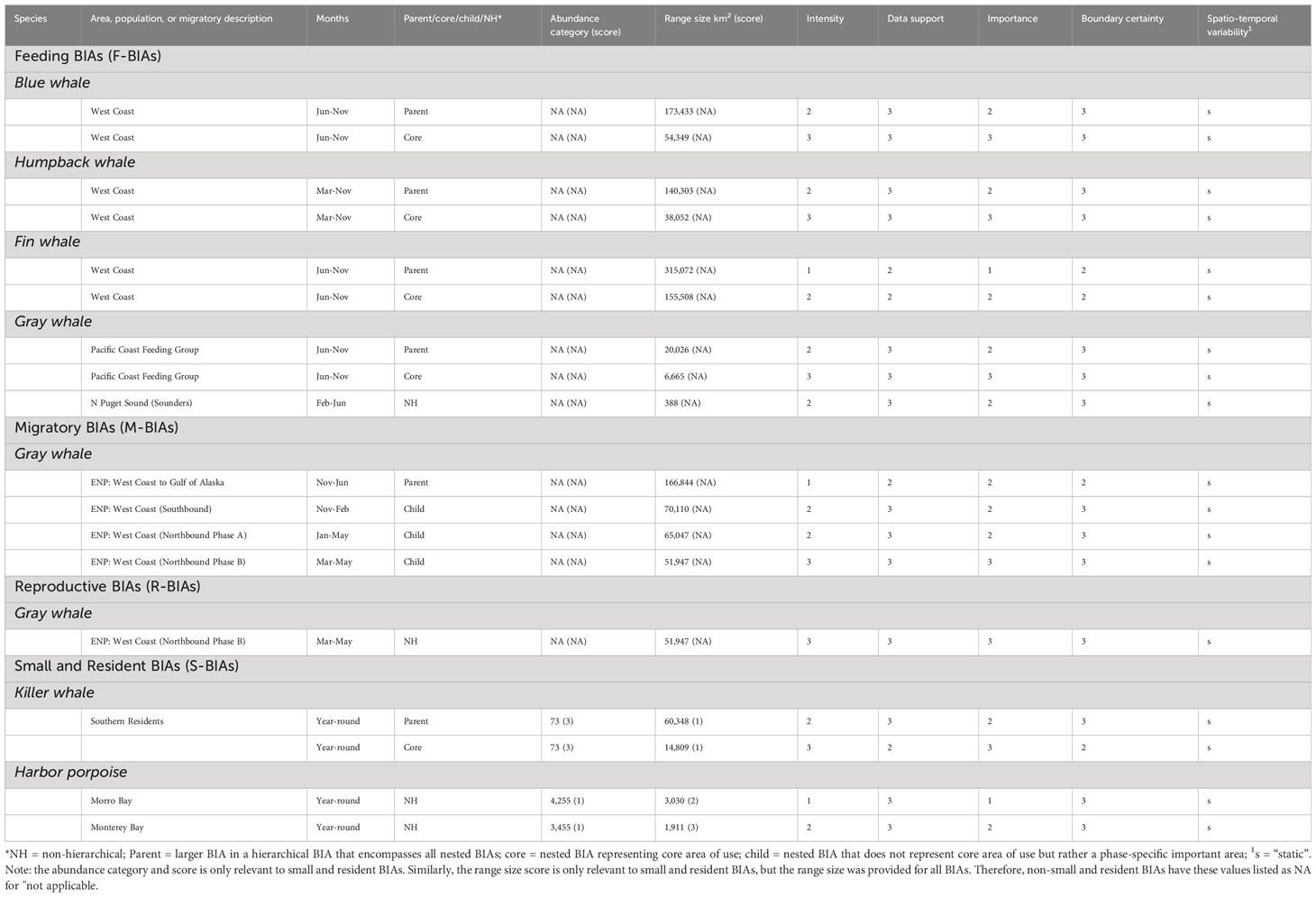
Table 1 Summary of types, species, areas, times, and key parameters and scores for the updated and newly delineated West Coast BIAs.

One important thing to note is the scoring assignments for the Spatiotemporal Variability Indicator. For many BIAs described here, particularly the F-BIAs, the species in consideration may respond to spatiotemporal variation in the environment and some of the habitat models for large whales have incorporated dynamic variables to account for this (Forney et al., 2012; Scales et al., 2017; Abrahms et al., 2019a; 2019b; Becker et al., 2020a; 2020b). More specifically, variability in oceanographic conditions along the West Coast region often results in variation in the spatial distribution of prey patches (e.g., krill, anchovies) upon which large whales feed. As such, these whales may adjust their feeding behavior in space and time accordingly. However, we assigned a Spatiotemporal Variability Indicator score of “static” for all BIAs here, for the following reasons: (1) for BIAs derived from the integrated approach, we intentionally attempted to account for year-to-year variability in whale distribution by using multi-year averaged HD model outputs; and (2) many of the BIAs’ spatial extents cover large areas, such that whale distribution within those areas may change in response to the environment, but the boundaries themselves are unlikely to move in space or time.

3 Results

Existing BIAs for many species described in Calambokidis et al. (2015) were revised to better align with the BIA protocols developed in this assessment (Harrison et al., 2023) and to make use of new data and analyses. In the sections that follow, we provided background information on each species and justified BIA delineation based on current understanding of their population structure and distribution from relevant published studies, stock assessment and technical reports, and/or unpublished information from the sources detailed above. We then described the data types and methods used to delineate new or update existing BIAs and reported summary information on each BIA in Table 1. While we provide full summaries and descriptions of the BIAs revised or delineated in this manuscript, for brevity, scores for all BIAs are reported in Table 1 and key highlights on scoring are provided in individual BIA sections. Comprehensive scoring narratives for all West Coast BIAs are provided in Supplementary Materials and are available on the BIA website¹. For the large whale F-BIAs, we also assessed how well revised (or new) BIAs captured important metrics from each data stream compared to the original BIAs delineated by Calambokidis et al. (2015), and these are reported in Table 2.

Table 2

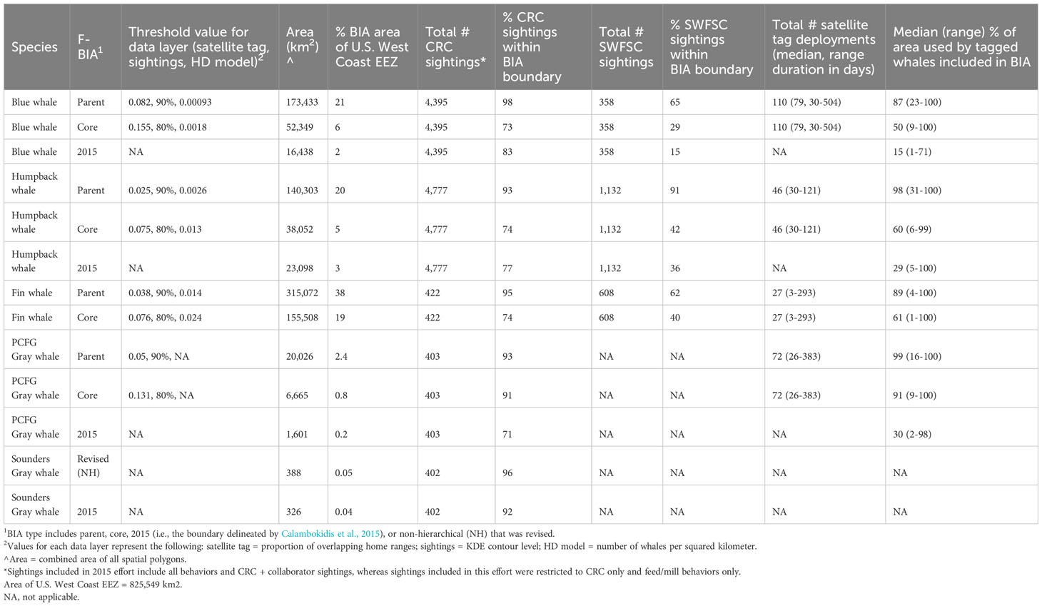
Table 2 Summary of key parameters for humpback, blue, fin, and gray whale BIAs updated or delineated here compared to previous BIAs delineated by Calambokidis et al. (2015) including threshold values (see methods), area, and summaries of how they encompassed proportions of sightings and tagged whale areas used.

3.1 Blue whale F-BIA

3.1.1 Background

Blue whales were initially spared as targets of early commercial whaling in the 1700 and 1800s due to their large size and speed but quickly became a primary target with the advent of modern whaling methods and ships starting in the early 20^th century. Due to rapid depletion throughout their range, the blue whale is listed as Endangered under the U.S. Endangered Species Act (ESA). Worldwide populations were reduced in the 20^th Century from over 200,000 to under 10,000 individuals, with most of those killed from the southern oceans (Gambell, 1976; Gambell, 1979). Blue whales in the North Pacific Ocean are thought to consist of at least a western/central and an eastern population based on distribution and vocalizations, although historically there may have been as many as five populations (National Marine Fisheries Service (NMFS), 1998). The eastern North Pacific blue whales range from the Costa Rica Dome to the Gulf of Alaska (Bailey et al., 2009; Calambokidis et al., 2009) and here we review the BIA status for this population off the U.S. West Coast.

Since the 1970s, large concentrations of blue whales have been documented feeding off California each summer and fall (Calambokidis et al., 1990). Relatively low numbers of blue whales were taken by whalers off the West Coast (Rice, 1963; 1974; Monnahan et al., 2014), so it was initially unclear how the animals feeding off the U.S. West Coast were related to those from the primary areas where they had been taken farther north off British Columbia, in the Gulf of Alaska, and in the Aleutians (NMFS, 1998). Shifts in blue whale distribution that occurred since the late 1990s, including documented movements of blue whales from California northward to areas off British Columbia and Alaska, have shown that blue whales inhabit a broad and shifting feeding area throughout the eastern North Pacific (Calambokidis et al., 2009). These changes in blue whale distribution appear related to decadal oceanographic variations because the timing coincided with shifts in the Pacific Decadal Oscillation (Calambokidis et al., 2009). Blue whale foraging intensity has also been shown to vary with decadal oceanographic variations off the U.S. West Coast (Palacios et al., 2019).

Blue whale total abundance in the eastern North Pacific estimated from capture-recapture of photo-identified individuals has only shown a slight increase since the 1990s with most recent estimates of about 2,000 (Calambokidis and Barlow, 2004; 2013; 2020). Density and average abundance of animals from line-transect surveys off the U.S. West Coast, however, have declined from about 1,400 in the early 1990s to 670 in 2018 (Barlow and Forney, 2007; Calambokidis and Barlow, 2013; Barlow, 2016; Becker et al., 2020b). These two methodologies provided different measures of abundance: data from line-transect surveys estimated the number of animals in the region during the survey period, whereas the photo-identification data provided estimates of the total population size. Differences in the line-transect estimates may be the result of fewer whales feeding off the U.S. West Coast and instead using other parts of their range (Calambokidis and Barlow, 2004; Calambokidis et al., 2009).

Blue whales along the U.S. West Coast face a number of anthropogenic threats (Carretta et al., 2022) but most importantly, vessel strikes have been identified as a significant source of mortality (Berman-Kowaleski et al., 2010; Redfern et al., 2013; Rockwood et al., 2017). Monnahan et al. (2014, 2015) concluded eastern North Pacific blue whales had recovered to pre-whaling abundance/carrying capacity levels and that current levels of ship strikes do not threaten their abundance, though this was based on a number of assumptions including absence of other threats or changes in environmental conditions. The initial blue whale F-BIAs from Calambokidis et al. (2015) were delineated through a qualitative assessment of sightings data relative to the best available habitat density model at the time. The 2015 F-BIAs are updated here with the more robust integrated approach and are more consistent with other regions (Harrison et al., 2023).

3.1.2 BIA boundary delineation and scoring

For this BIA, we implemented the integrated approach detailed in the Methods section, incorporating CRC sightings data (Calambokidis et al., 2015; CRC, Unpublished), OSU satellite tag data (Irvine et al., 2014; Mate et al., 2018), and SWFSC HD model predictions (Becker et al., 2020a, 2020b; Figure 1; Supplementary Table 3). This F-BIA spans June through November which is the primary feeding period for blue whales in this region (Calambokidis et al., 2009; Irvine et al., 2014; Širović et al., 2015; Derville et al., 2022). The new BIA is shown in Figure 2, and details on the spatiotemporal specifications and scoring are provided in Table 1. Threshold cut-off values for each layer are shown in Figure 2 and reported in Table 2. The inner (shoreward) boundary of the parent BIA was defined as the 50-m depth contour and the inner boundary of the core BIA was defined as the 80-m depth contour, based on major drops in the frequency of sightings in small boat efforts at those depths (see Supplementary File A, Section S2.5, Supplementary Figure 2). There was weak evidence for differences in the spatial distribution of feeding blue whale sightings with and without calves (Supplementary File A, Section S2.6, Supplementary Figures 5, 6), and thus no R-BIA was delineated for blue whales.

Figure 1

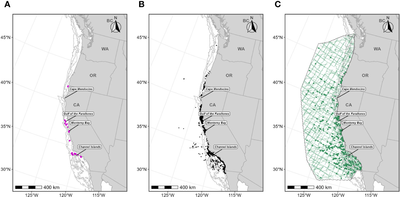
Figure 1 Individual data sources used in blue whale F-BIA boundary determinations: (A) OSU blue whale satellite tag deployment locations (magenta circles) for which HRs were estimated (n=110) from 1998-2017; (B) CRC blue whale sightings (black points) with observed feeding/milling behaviors (n=4,395) from dedicated small boat survey efforts from 1986 through 2020 during the feeding season (June-November); (C) SWFSC HD model prediction study area (black outline) encompassing line-transect surveys (green lines) conducted from 1991 through 2018, and blue whale sightings from these surveys shown as green circles. Depth contours (200 m, 1,000 m, and 2,000 m) are shown as light grey lines.

Figure 2

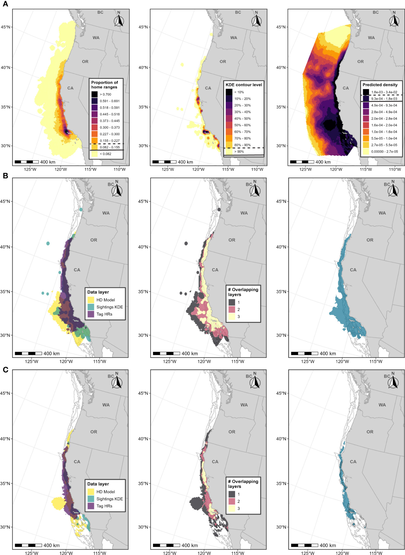
Figure 2 Boundary determination for blue whale F-BIAs on the West Coast. (A) Individual data layers used in BIA boundary determinations: (left) proportion of all blue whale HRs derived from satellite tag data; (center) blue whale feeding/milling sightings KDE; (right) HD model predictions averaged over 1991-2018; threshold values used in BIA delineation are indicated in the legend keys for each data layer (parent = solid line, core = dashed line). (B) Parent BIA boundary delineation: (left) subsetted data layers based on threshold values shown in (A) for each data layer; (center) overlap among subsetted data layers; (right) resulting parent BIA boundary based on areas with at least 2 overlapping polygons. (C) Core BIA boundary delineation: (left) subsetted data layers based on threshold values shown in (A) for each data layer; (center) overlap among subsetted data layers; (right) resulting core BIA boundary based on areas with at least 2 overlapping polygons. The shoreward boundaries for the parent and core BIAs were defined by the 50-m and 80-m depth contours, respectively. 2015 boundaries are outlined in black. Depth contours (200 m, 1,000 m, and 2,000 m) are shown in light grey lines.

In general, the parent blue whale F-BIA was assigned a lower Intensity score compared to the core F-BIA to reflect the differences in intensity of use between the two BIAs. This BIA has strong data support as it was derived from three extensive independent datasets spanning over 35 years through an integrated approach that complements the strengths and weaknesses of each data source. There are no other blue whale F-BIAs delineated for the eastern North Pacific population of blue whales. The resulting scores reflect our knowledge of feeding blue whales in this region and the data and methods used to delineate this BIA. A full narrative of the scoring is provided in Supplementary File B.

3.1.3 Area and level of inclusion of parent and core BIAs delineated

Parent BIAs for blue whales covered 173,000 km² or 21% of the U.S. West Coast EEZ and encompassed portions of coastal waters, shelf edge, and some offshore habitats (Table 2). This parent BIA successfully encompassed 98% of the CRC sightings of feeding whales, 65% of the sightings from SWFSC sightings, and a median of 87% of the area used by tagged blue whales (Table 2). While the previously described BIA (Calambokidis et al., 2015) encompassed a high proportion of the CRC feeding sightings (83%), it did a poor job of capturing the SWFSC sightings (15%), or the area used by tagged whales (15%) since those layers were not considered in the first delineation process (Calambokidis et al., 2015).

The core BIA represented 30% of the parent BIA but was still larger than the previous BIA (Table 2). Despite this smaller size, the core BIA encompassed 73% of the feeding sightings. Although it only encompassed a median of 50% of the area used by tagged animals and 29% of the SWFSC sightings, these values exceeded those of the previous 2015 BIA, which did not consider the tag or SWFSC line-transect data layers for BIA development (Table 2).

3.2 Humpback whale F-BIA

3.2.1 Background

Humpback whales are one of the most common and abundant large cetaceans in coastal waters of the U.S. West Coast. They were depleted by hunting during the modern era of commercial whaling including through 1966 from whaling stations along the U.S. West Coast. In the North Pacific Ocean, humpback whales migrate between winter breeding areas including those in the western North Pacific Ocean, Hawaiʻi, Mexico, and Central America, and more coastal feeding areas in spring, summer, and fall that range from California, north into Alaskan waters and west to waters off Russia (Calambokidis et al., 2001, 2008). Both photo-identification and genetic data indicate that, in the North Pacific Ocean, humpback whales remain loyal to specific feeding and wintering areas, although their migrations between these areas reveal a mixed stock structure (Calambokidis et al., 2008; Barlow et al., 2011; Baker et al., 2013).

Off the U.S. West Coast, humpback whales are most abundant from spring through fall, with most migrating to low-latitude areas located primarily off Mexico and Central America in winter (Calambokidis et al., 2000). However, sightings and passive acoustic detections off the U.S. West Coast in winter and spring indicate a portion of the population can be in northern waters through the winter (Forney and Barlow, 1998; Oleson et al., 2009). There are also indications of seasonal shifts in occurrence both up and down the coast as well as inshore and offshore (Campbell et al., 2015; Fleming et al., 2015; Becker et al., 2017; Derville et al., 2022). During small-boat surveys off the Washington coast in 2004-2008, humpback whales were seen farther offshore (along the shelf edge) and in lower densities in winter and spring than during the remainder of the year (Oleson et al., 2009). Humpback whale distribution off Oregon and northern California and the relationship with environmental variables differed by season (Tynan et al., 2005).

Interchange between the humpback whale feeding aggregation off California/Oregon and those off Washington and southern British Columbia is much lower than within these regions (Calambokidis et al., 1996, 2000, 2001, 2004, 2008). Similarly, studies have confirmed dramatic genetic (mtDNA) differences between these two areas (Baker et al., 2008). For this reason, abundance estimates from mark-recapture of photographically identified individuals have been conducted separately for these areas (Calambokidis and Barlow, 2004, 2013, 2020). Abundance of humpback whales off California/Oregon has increased dramatically since late 1980s at about 7-8% per year and now numbers close to 5,000 (Calambokidis and Barlow, 2020). Estimates for Washington/southern British Columbia have increased even more rapidly and most recently numbers 1,000-1,500 (Calambokidis and Barlow, 2020).

Humpback whales that feed off the U.S. West Coast migrate primarily to wintering grounds off mainland Mexico, Central America, and Hawaiʻi (Calambokidis et al., 2000, 2008; Wade et al., 2016) though with a shifting proportion by latitude. Humpback whales wintering off Central America have significant differences in mtDNA haplotypes from other North Pacific wintering areas, including mainland Mexico (Baker et al., 2008, 2013) though these differences do not allow assignment of whales to winter breeding areas based solely on genetics (Martien et al., 2020). Due to differences in genetics and more limited interchange from photo-identification, humpback whale winter breeding areas in the North Pacific (Bettridge et al., 2015) are designated by NOAA as having four Distinct Population Segments (DPS) under the U.S. ESA: 1) Central America DPS, recognized as Endangered, 2) Mexico DPS, recognized as Threatened, 3) Hawaiʻi DPS, no longer listed, and 4) Western North Pacific DPS, recognized as Endangered. Humpback whales in our BIAs include whales from the first three of these DPSs, meaning they include whales considered Endangered, Threatened and not listed under the ESA. Additionally, there might be an occasional presence of whales from the Western North Pacific DPS since one whale from this DPS has been seen along the Washington/British Columbia border (Darling et al., 1996).

The Central America DPS was estimated to consist of <1,000 whales in the mid-2000s (the reason for its Endangered status) and almost exclusively migrates to the U.S. West Coast feeding areas (Calambokidis et al., 2008; Rasmussen et al., 2011; Wade et al., 2016; Wade, 2017). More recent estimates indicate an abundance of closer to 1,500 (Curtis et al., 2022). Even though humpback whales along the U.S. West Coast have been increasing, they face a number of anthropogenic threats (Carretta et al., 2022). Vessel strikes have been increasingly identified as a source of mortality of a number of large whale species, including humpback whales, worldwide, but this problem is heightened where key feeding areas overlap with areas of high vessel traffic as occurs in several areas along the U.S. West Coast (Redfern et al., 2013; Rockwood et al., 2017). Humpback whale entanglements have increased dramatically off the U.S. West Coast since the mid-2010s (Saez et al., 2021; NOAA, 2023).

Potential Impacts to this Endangered DPS from anthropogenic threats like entanglements or ship strikes off the U.S. West Coast are of great concern. Photo-identification data indicates the proportion of humpback whales belonging to each DPS varies along the U.S. West Coast with the highest proportion of whales from the Endangered Central America DPS occurring in southern California and decreasing northward as the proportion from the Mexico and Hawaiʻi DPS increases (Calambokidis et al., 2000, 2008, Unpublished).

NOAA developed and listed Critical Habitat for humpback whales along the U.S. West Coast in 2021 (NOAA, 2021) partly in response to concerns about entanglements and other threats. We did not specifically use Critical Habitat in our delineation of BIAs since these were based on different criteria. Our parent BIA is smaller than the area designated as Critical Habitat but does include some areas that were excluded from Critical Habitat due national security considerations, such as the Navy’s Quinault Range Site (plus a buffer zone).

3.2.2 BIA boundary delineation and scoring

For the humpback whale F-BIAs in this region, we implemented the integrated approach detailed in the Methods section, incorporating CRC sightings data, OSU satellite tag data (Palacios et al., 2020), and SWFSC HD model predictions (Becker et al., 2020a, 2020b; Figure 3; Supplementary Table 3). This F-BIA spans March through November which is the primary feeding period for humpback whales in this region (Carretta and Forney, 1993; Calambokidis et al., 2000; Becker et al., 2017; Derville et al., 2022). The new BIA is shown in Figure 4, and details on the spatiotemporal specifications and scoring are provided in Table 1. Threshold cut-off values for each layer are shown in Figure 4 and Table 2. The inner boundary of the parent BIA was defined as the 30-m depth contour and the inner (shoreward) boundary of the core BIA was defined as the 70-m depth contour, based on major drops in the frequency of small boat sightings below those depths (see Supplementary File A, Section S2.5, Supplementary Figure 3). There was weak evidence for differences in the distribution of feeding humpback whales with and without calves (Supplementary File A, Section S2.6, Supplementary Figures 7, 8), and thus no R-BIA was delineated for humpback whales.

Figure 3

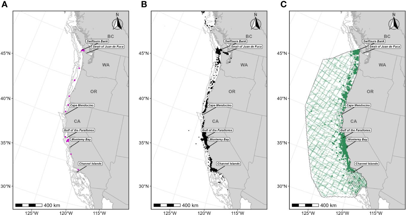
Figure 3 Individual data sources used in humpback whale F-BIA boundary determinations. (A) OSU humpback whale satellite tag deployment locations (magenta circles) for which HRs were estimated (n=41) from 2004-2019; (B) CRC humpback whale sightings (black points) with observed feeding/milling behaviors (n=4,777) from dedicated small boat survey efforts from 1986 through 2020; (C) SWFSC HD model prediction study area (black outline) and encompassing line-transect surveys (green lines) conducted from 1991 through 2018, and humpback whale sightings from these surveys shown as green circles. Depth contours (200 m, 1,000 m, and 2,000 m) are shown as light grey lines.

Figure 4

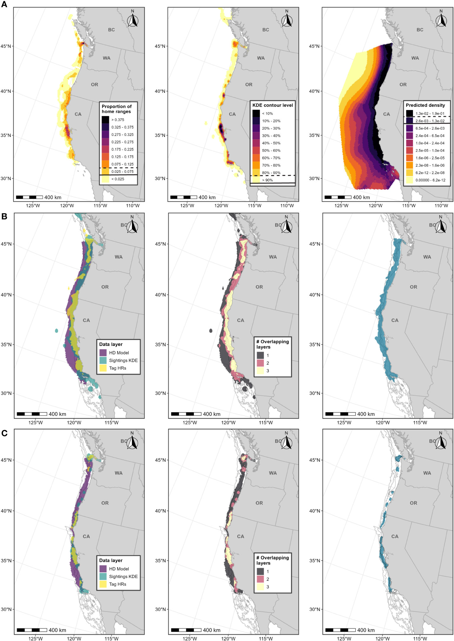
Figure 4 Boundary determination for humpback whale F-BIAs on the West Coast. (A) Individual data layers used in BIA boundary determinations: (left) proportion of all humpback whale HRs derived from satellite tag data; (center) humpback whale feeding/milling sightings KDE; (right) HD model predictions averaged over 1991-2018; threshold values used in BIA delineation are indicated in the legend keys for each data layer (parent = solid line, core = dashed line). (B) Parent BIA boundary delineation: (left) subsetted data layers based on threshold values shown in (A) for each data layer; (center) overlap among subsetted data layers; (right) resulting parent BIA boundary based on areas with at least 2 overlapping polygons. (C) Core BIA boundary delineation: (left) subsetted data layers based on threshold values shown in (A) for each data layer; (center) overlap among subsetted data layers; (right) resulting core BIA boundary based on areas with at least 2 overlapping polygons. The shoreward boundaries for the parent and core BIAs were defined by the 30-m and 70-m depth contours, respectively. 2015 boundaries are outlined in black. Depth contours (200 m, 1,000 m, and 2,000 m) are shown in light grey lines.

Scores for this BIA are provided in Table 1 and narratives are provided in Supplementary File B and on the BIA website. Scoring for the humpback whale F-BIA were the same as those for the blue whale F-BIA due to similar reasons, primarily the known intensity of use of the areas defined by the BIAs for feeding and the substantial support by all data sources used to delineate the BIA.

3.2.3 Area and level of inclusion of parent and core BIAs delineated

The combined layers and the use of a depth criterion results in a parent BIA of 140,000 km² representing 20% of the area of the U.S. West Coast EEZ (Table 2). This parent BIA successfully encompassed 93% of the CRC sightings of feeding whales, 91% of the sightings from SWFSC sightings, and a median 98% of the area used by tagged humpback whales (Table 2). While the previous BIA (Calambokidis et al., 2015) encompassed a high proportion of the CRC feeding sightings (77%), it did a poor job of capturing the SWFSC sightings (36%), or the area used by tagged whales (29%) since those layers were not considered.

The core BIA represented 27% of the parent BIA but was still a little over 50% larger than the original 2015 BIAs (Table 2). The core BIA encompassed 74% of the feeding sightings, though only a median of 60% of the area used by tagged whales and 42% of the SWFSC sightings; the new core BIA nonetheless included higher proportions than the 2015 BIA that did not consider those data layers (Table 2).

3.3 Fin whale F-BIA

3.3.1 Background

Fin whales are widely distributed through the world’s oceans including northern and southern hemispheres. In the eastern North Pacific, fin whales occur from the tropical Pacific up to Arctic waters (Mizroch et al., 2009) and the fin whales off California, Oregon, and Washington are treated as a single stock (Carretta et al., 2022). In general, their migrations and population structure are less well understood than for blue or humpback whales, but numbers are generally higher in summer/fall compared to winter/spring especially off southern California (Douglas et al., 2014; Campbell et al., 2015). Abundance estimates of fin whales off the U.S. West Coast show increasing numbers since the early 1990s (Moore and Barlow, 2011) and now are estimated at 11,065 (Becker et al., 2020b; Carretta et al., 2022). Fin whales along the U.S. West Coast face a number of anthropogenic threats (Carretta et al., 2022). Rockwood et al. (2017) estimated that ship-strike mortality for fin whales was 2.7x above the potential biological removal (PBR) limit set by NMFS. While fin whales are always at risk of ship-strike, the diving behavior of fin whales at night increases their risk of a strike twofold over daytime (Calambokidis et al., 2019a; Keen et al., 2019).

Additional data in recent years have helped examine the movements and population status of fin whales off the U.S. West Coast. Fin whales in the Southern California Bight (SCB) tended to occur closer to shore in shallower waters in Winter/Spring compared to Summer/Fall (Douglas et al., 2014; Scales et al., 2017; Falcone et al., 2022). Irvine et al. (2019) reported the movements and feeding behavior of five fin whales tagged with medium-duration archival tags in the nearshore waters of the SCB and which largely stayed in that region. Scales et al. (2017) reported the results of 67 deployments of medium- duration satellite tags deployed mostly in the SCB but also off Washington and which ranged from southern Baja California to northern Vancouver Island while tagged. A different set of medium-duration archival tags deployed on fin whales mostly off southern California also showed feeding and fairly limited movements in the SCB though one whale moved from the California/Oregon border north to off Vancouver Island in a few weeks (Calambokidis et al., 2019a; CRC, Unpublished data).

Falcone et al. (2022) using long-term photo-ID data suggest the existence of two overlapping groups of fin whales off the U.S. West Coast including a year-round resident group in the SCB that shifts inshore/offshore seasonally and a more transient group with broader seasonal movements ranging much farther north. Fin whale vocalizations also show changes both through the season and across years supporting the hypothesis of two possible populations (Širović et al., 2013; 2015; 2017). Genetic data from fin whales also suggested the possible existence of multiple populations in the eastern North Pacific with a possible north/south separation (Archer et al., 2013; 2019).

BIAs for fin whales were not delineated in the previous round of BIA determinations due to inadequate data, but fin whale distribution was discussed (Calambokidis et al., 2015). Given the availability of additional data, we were able to designate BIAs for fin whales in this round using the integrated multiple data approaches employed for other large whale species, but applying a weighting scheme to account for the variability in the strength of the data layers. Specifically, we weighted the HD models more heavily than with blue and humpback whales because they more consistently covered the entire U.S. West Coast including offshore waters compared to the small-boat sightings or the satellite tag deployments.

3.3.2 BIA boundary delineation and scoring

For this BIA, we implemented the integrated approach detailed in the Methods section, incorporating CRC sightings data, OSU and MarEcoTel satellite tag data (Scales et al., 2017; Falcone et al., 2018; Mate et al., 2018; 2022), and SWFSC HD model predictions (Becker et al., 2020a; 2020b; Figure 5, Supplementary Table 3). Medium-duration archival data from Irvine et al. (2019) and Calambokidis et al. (2019a) were not incorporated due to limited sample size and because these tags collected data over much shorter time periods (1-2 weeks) than the other tracking data we included and thus could bias delineation of important areas towards the areas where these tags were deployed. The integrated approach was modified for this BIA to place more weight on the HD model layer; the shipboard line-transect surveys used to support the HD models covered regions where fin whales are more likely to occur (farther offshore) and where other data sources may be limited (Becker et al., 2020a; 2020b). The HD model layer was also derived from a comparatively large sample size of visual sightings (n=608; Table 2). As such, the fin whale BIAs (parent and core) were defined as the entire HD model layer (after applying thresholds) in addition to all other areas where both the small boat sighting and satellite tag data layers overlapped (Figure 6). The integration method for the other large whale F-BIAs places equal weight among all data layers, whereby overlap between any two data layers (or more) would be incorporated into the BIA. Therefore, including the entire HD model layer in the fin whale BIA regardless of whether another data layer overlapped with it in space places more weight on this layer in the delineation process, and more explicitly incorporates the advantages of the HD model layer for this species. This F-BIA spans June through November which is the primary feeding period for fin whales in this region (Douglas et al., 2014; Širović et al., 2015; Scales et al., 2017; Derville et al., 2022; Falcone et al., 2022; Table 1). Although fin whales have been documented in this region during winter and spring months (Scales et al., 2017; Derville et al., 2022; Falcone et al., 2022), and some indication of seasonal differences in distribution (Douglas et al., 2014), data availability was limited during the winter/spring and thus not adequate to do an independent distribution layer for that period. Future BIA efforts should evaluate this temporal parameter as additional information is obtained on fin whale temporal occurrence off the U.S. West Coast. Threshold values for each layer are shown in Figure 6 and listed in Table 2. The inner (shoreward) boundary of the parent BIA was defined as the 60-m depth contour and the inner boundary of the core BIA was defined as the 80-m depth contour, based on the depth frequency of small boat sightings (see Supplementary File A, Section S2.5, Supplementary Figure 4). There were very few CRC sightings of fin whales with calves from which we could compare spatial distributions of sightings for a candidate R-BIA (Supplementary File A, Section S2.6).

Figure 5

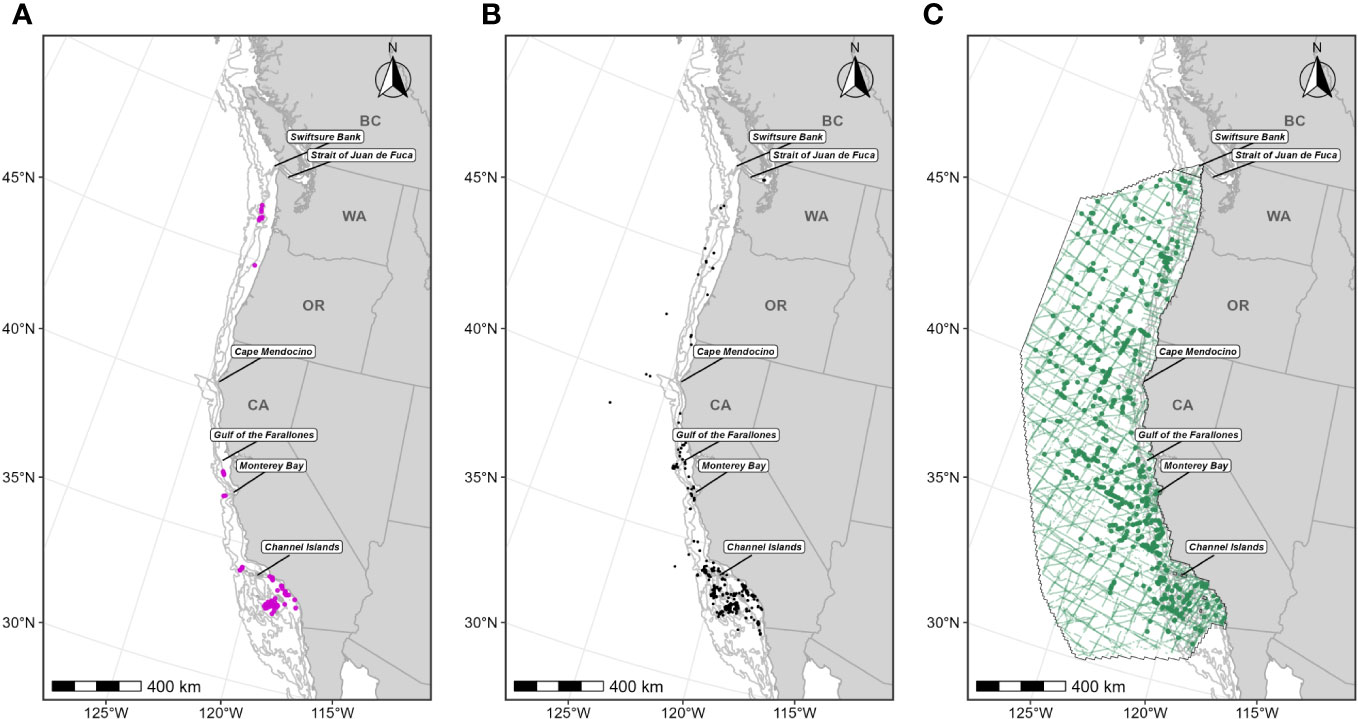
Figure 5 Individual data sources used in fin whale F-BIA boundary determinations: (A) OSU and MarEcoTel fin whale satellite tag deployment locations (magenta circles) for which HRs were estimated (n=79) from 2006-2018; (B) CRC fin whale sightings (black points) with observed feeding/milling behaviors (n=422) from dedicated small boat survey efforts from 1986 through 2020 during the feeding season (June-November); (C) SWFSC HD model prediction study area (black outline) encompassing line-transect surveys (green lines) conducted from 1991 through 2018, and fin whale sightings (n=608) from these surveys shown as green circles. Depth contours (200 m, 1,000 m, and 2,000 m) are shown as light grey lines.

Figure 6

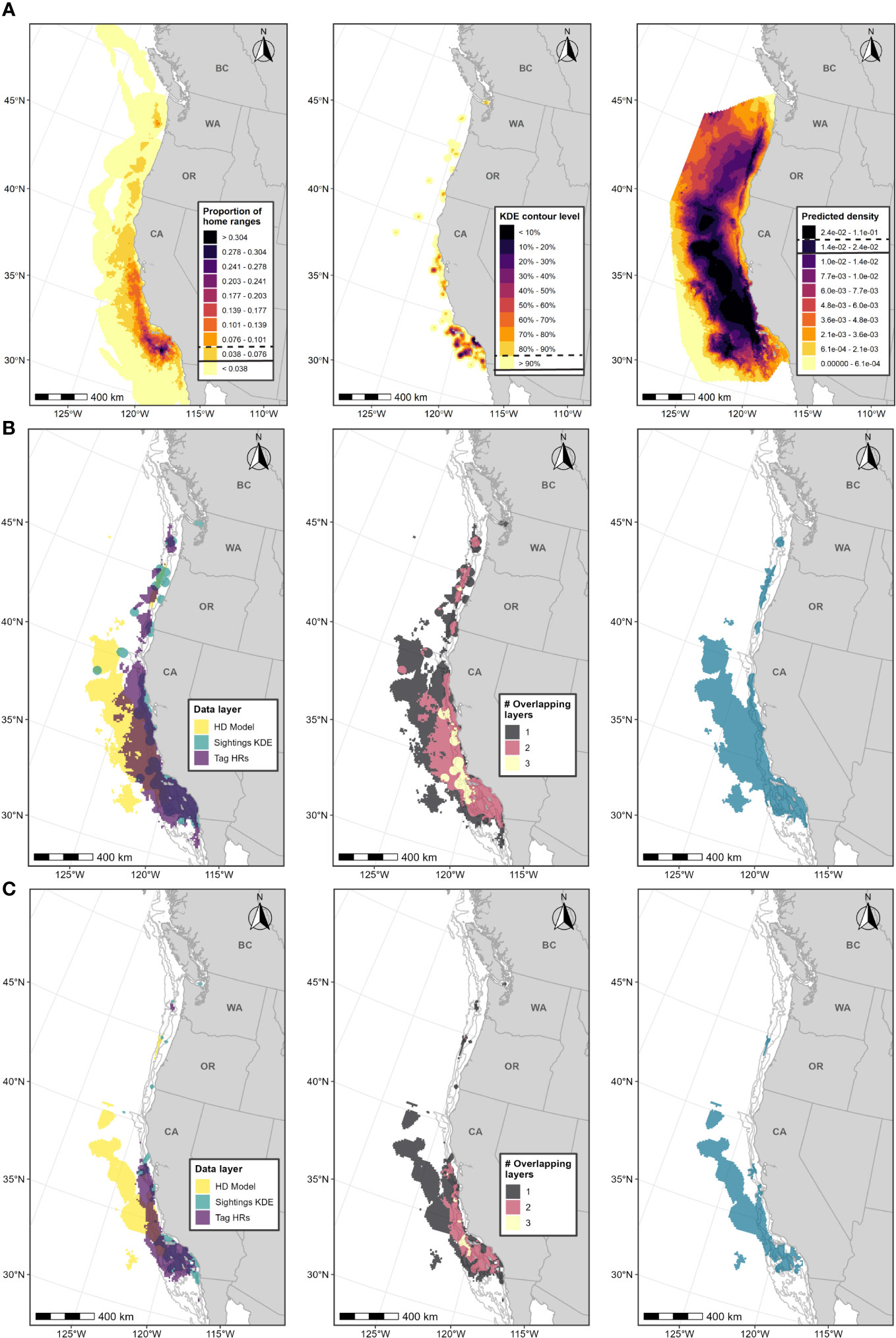
Figure 6 Boundary determination for fin whale F-BIAs on the West Coast. (A) Individual data layers used in BIA boundary determinations: (left) proportion of all fin whale HRs derived from satellite tag data; (center) fin whale feeding/milling sightings KDE; (right) HD model predictions averaged over 1991-2018; threshold values used in BIA delineation are indicated in the legend keys for each data layer (parent = solid line, core = dashed line). (B) Parent BIA boundary delineation: (left) subsetted data layers based on threshold values shown in (A) for each data layer; (center) overlap among subsetted data layers; (right) resulting parent BIA boundary based on the HD model layer plus areas with at least 2 overlapping polygons. (C) Core BIA boundary delineation: (left) subsetted data layers based on threshold values shown in (A) for each data layer; (center) overlap among subsetted data layers; (right) resulting core BIA boundary based on the HD model layer plus areas with at least 2 overlapping polygons. The shoreward boundaries for the parent and core BIAs were defined by the 60-m and 80-m depth contours, respectively. Depth contours (200 m, 1,000 m, and 2,000 m) are shown in light grey lines.

Scores for this BIA are provided in Table 1 and narratives are provided in Supplementary Materials and on the BIA website. Overall, the scores for the fin whale F-BIA were lower compared to the other large whale F-BIAs for the West Coast region. This was primarily attributed to the large size of both the parent and core BIAs for fin whales (nearly three times larger than other F-BIAs; Table 2) and comparatively limited understanding of fin whale distribution and feeding behavior within West Coast waters. For example, in contrast to the CRC sightings and satellite tag data layers, the HD model layer identified intensified areas of use much farther offshore for a majority of the West Coast region (Figures 5, 6). These areas overlap the spatial predictions of suitable habitat identified in Scales et al. (2017).

3.3.3 Area and level of inclusion of parent and core BIAs delineated

The combined layers and the use of depth criteria results in a parent BIA of 315,000 km² representing 38% of the area of the U.S. West Coast EEZ and the largest area of all the BIAs designated for the U.S. West Coast (Table 2). Such a large area reflected both coastal and extensive offshore use by fin whales along the U.S. West Coast. This parent BIA successfully encompassed 95% of the CRC sightings of feeding whales, 62% of the sightings from SWFSC sightings, and a median of 89% of the area used by tagged fin whales (Table 2). The core area BIA represented 49% of the overall parent BIA but encompassed 74% of the CRC feeding sightings, 40% of the SWFSC sightings, and 61% of the median tagged animal area.

The large size of the BIAs for fin whales makes it challenging to identify more precise critical areas compared to some of the other large whale species. As additional data become available, there may be better ways to delineate key core areas. Additionally, while there is some indication of more than one possible population of fin whales using the U.S. West Coast (Archer et al., 2013; Scales et al., 2017; Falcone et al., 2022), we did not have a way to specifically incorporate that into our BIAs - this should be an important consideration as more population-specific data become available. While a small proportion of our fin whale BIAs extend into Mexico, our ability to extend this BIA to any existing important feeding areas further south in Mexico waters was restricted by the lack of relevant data outside U.S. waters.

3.4 Gray whale BIAs

3.4.1 Background

Gray whales currently occur in the North Pacific making long migrations between winter breeding areas in the south and feeding areas at more northern latitudes (Rice and Wolman, 1971; Jones and Swartz, 1984). The overall Eastern North Pacific gray whale population has shown remarkable recovery from historical whaling but has also experienced multiple mortality events and large fluctuations in abundance (Stewart and Weller, 2021; Stewart et al., 2023). There is some current debate about how to define their population structure. In the past, Eastern and Western North Pacific populations were recognized, with the Eastern population wintering around Baja California, Mexico, and the Western population thought to use wintering areas somewhere in the South China Sea (Rice and Wolman, 1971; Weller et al., 2002). More recently, satellite tagging and photo-identification have revealed that many of the whales feeding in the Western North Pacific (e.g. Sakhalin Island, Russia) migrate along the U.S. West Coast on route to the Eastern North Pacific (ENP) wintering ground off Baja California (Weller et al., 2012; Mate et al., 2015), raising questions about the current status of Western North Pacific gray whales as a distinct unit. We consider below different BIAs for the following:

1. A hierarchical M-BIA for the migration corridor of the ENP gray whale population that is likely also used by Western North Pacific gray whales migrating to the Mexican wintering areas.

2. An R-BIA for the specific nearshore migratory corridor used late in the northbound migration disproportionally by mothers with calves.

3. F-BIAs for the Pacific Coast Feeding Group (PCFG) that spends the spring through fall feeding in the Pacific Northwest.

4. An F-BIA for the gray whales that repeatedly use a small area in northern Puget Sound each spring to feed intensely on ghost shrimp before appearing to continue their migration to the Arctic with the rest of the ENP gray whales (recently termed the “Sounders” gray whales).

The PCFG is a trans-boundary subgroup observed almost year-round primarily from spring to fall, numbers several hundred, and returns annually and feeds in coastal waters of the Pacific Northwest (Calambokidis et al., 2002; 2014). Genetic differences are evident between this group and other gray whales including those feeding in the Bering Sea (Frasier et al., 2011; Lang et al., 2014). They are considered a distinct stock in Canada although currently are not treated as a distinct stock in the NMFS Stock Assessment Reports (Weller et al., 2013). During the migration, PCFG whales are intermixed with the larger ENP population; however, from June to November, PCFG whales are the only gray whales within the region between northern California and northern Vancouver Island (from 41°N to 52°N) (Calambokidis et al., 2002, 2010, 2014, 2019; International Whaling Commission, 2011; Lagerquist et al., 2019). PCFG gray whales are also occasionally seen in waters farther north during summer and autumn, including off Kodiak Island, Alaska (Gosho et al., 2011; Lagerquist et al., 2019). The primary feeding areas for ENP gray whales are thought to be in the Bering, Chukchi, and Beaufort seas, while WNP gray whales are thought to feed primarily near Sakhalin Island, Russia, in the Okhotsk Sea. Therefore, proposed F-BIAs in U.S. West Coast waters focus on the PCFG gray whales.

We also designate an F-BIA in northern Puget Sound for a feeding area for one group of ENP gray whales, termed the “Sounders” gray whales, which annually use the south end of Whidbey and Camano islands (Calambokidis et al., 2015; Calambokidis, 2016). Gray whales come to this area for two to three months in the spring (typically beginning in March) to feed, but then generally leave the area before 1 June and, therefore, are not treated as PCFG gray whales (Calambokidis et al., 1992; 2002). While this area is not used by many individuals, the same animals have been documented to return to this relatively small area for over 30 years and it may therefore be important for this group (Calambokidis et al., 2014).

One distinction of the gray whale BIAs from the rest of the large whale BIAs is the absence of an inner (shoreward) bound defined by a depth contour. Because gray whales are often seen very close to shore in shallow waters (Table 3), a defined inner boundary based on a depth contour was not deemed necessary for these BIAs.

Table 3

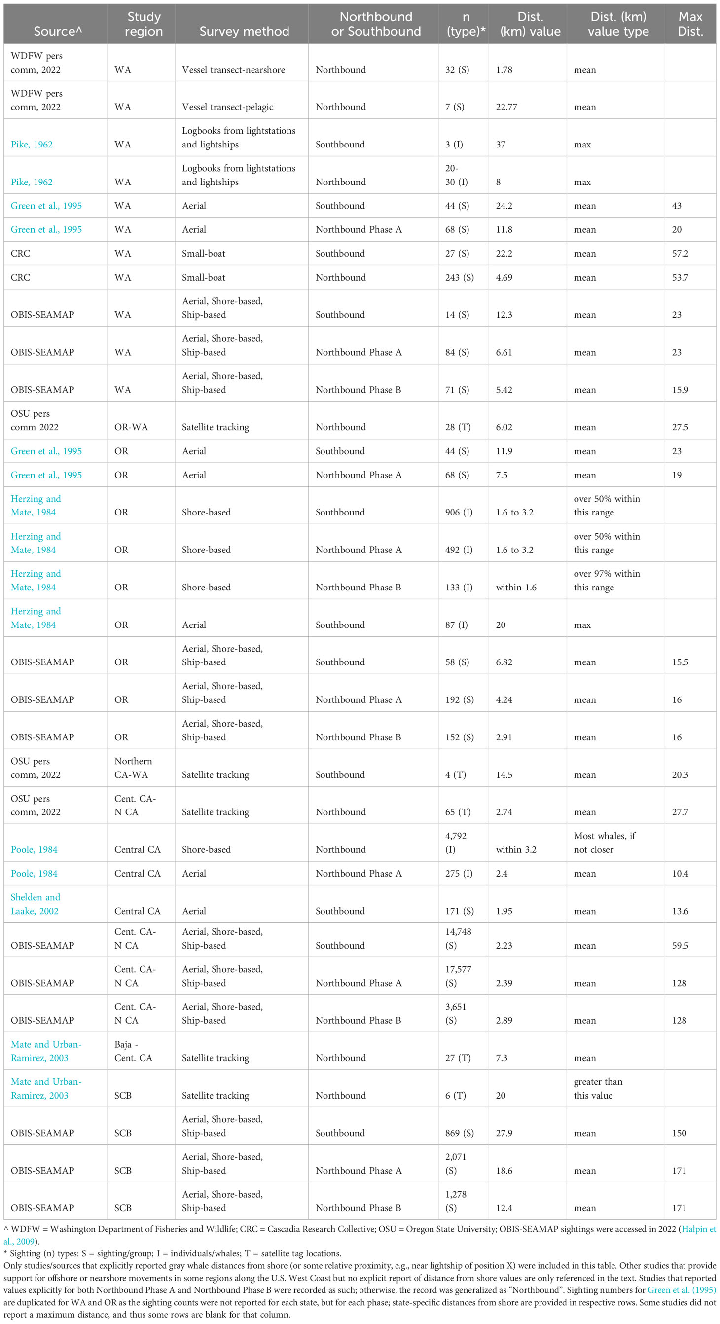
Table 3 Summary of distributions (distance from shore) of migratory gray whales along the U.S. West Coast from existing literature and other datasets made available for this effort.

3.4.2 PCFG gray whales: F-BIA boundary delineation and scoring

For the PCFG gray whale F-BIA, we implemented the integrated approach detailed in the Methods section, incorporating CRC sightings data and OSU satellite tag data (Lagerquist et al., 2019; no HD model output are available; Figure 7, Tables 1, 2, Supplementary Table 3). Threshold values for each layer are described in the Supplementary Material and shown in Figure 7 and Table 2.

Figure 7

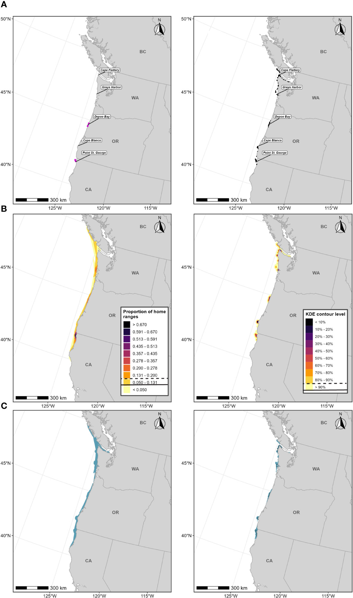
Figure 7 Boundary determination for PCFG gray whale F-BIAs on the West Coast. (A) Individual data sources (left) OSU PCFG gray whale satellite tag deployment locations (magenta circles) for which HRs were estimated for (n=23) from 2009-2013 and (left) CRC gray whale sightings (black points) with observed feeding/milling behaviors (n=403) from dedicated small boat survey efforts from 1992 through 2020 during the PCFG feeding season (June-November). (B) Individual data layers used in BIA boundary determinations: (left) Proportion of all PCFG gray whale HRs derived from satellite tag data and (right) PCFG gray whale sightings KDE; threshold values used in BIA delineation are indicated in the legend keys for each data layer (parent = solid line, core = dashed line). (C) Revised F-BIAs for PCFG gray whales: (left) parent BIA and (right) core BIA. 2015 boundaries are outlined in black.

Scores for this BIA are provided in Table 1 and justified in the Supplementary Material and BIA website. The scoring and justifications for this BIA mirrored those for the blue whale and humpback whale F-BIAs, which had generally high scores all around based on the supporting data sources, current understanding of their use of the delineated BIAs for feeding, and the approach implemented to determine the spatial extents of the BIA boundaries.

3.4.3 Sounders gray whales: F-BIA boundary delineation and scoring

Sightings data collected from dedicated small boat survey efforts by CRC from 1994-2020 (n=402 feeding or milling gray whales) were used to revise the existing F-BIA boundary for the Sounders gray whales occurring in northern Puget Sound. Based on the distribution of the more recent sightings and expert elicitation, the 2015 BIA boundary was expanded to include Holmes Harbor and farther north into Port Susan (Figure 8). The 2015 Sounders gray whale BIA spanned the months March through May; given recent documentation of Sounders gray whale use of northern Puget Sound both earlier than March and later than May (CRC, Unpublished), we expanded the feeding season for this BIA to cover February through June.

Figure 8

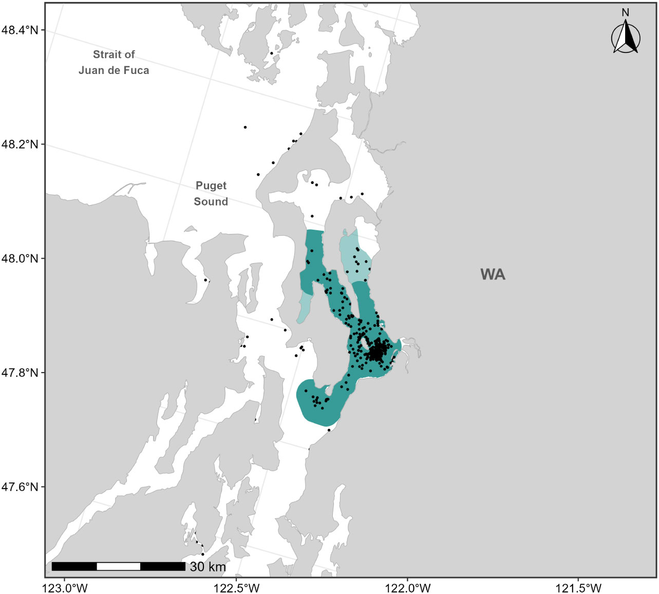
Figure 8 Feeding BIA boundary for the “Sounders” gray whales in Northern Puget Sound spanning February through June; the dark shaded polygon represents the boundary delineated by Calambokidis et al. (2015) and the light shaded polygons represent the extensions added to the 2015 boundary in this assessment (total polygon area is the revised BIA). Sightings of feeding gray whales are shown as black points (n=402).

Scoring for the Northern Puget Sound gray whale F-BIA is summarized in Table 1 and more specific details and narratives are provided in Supplementary Materials and on the BIA website. While this BIA reflects important feeding grounds for a small number of individuals over a relatively short period (and thus is indicative of high intensity), we assigned an Intensity score of 2 for the BIA rather than a higher score of 3. This is primarily because this feeding area appears to be more of a temporary foraging ground for a subset of ENP gray whales, which, after spending time in northern Puget Sound, leave and continue on their migration north presumably to Arctic feeding grounds. Therefore, the northern Puget Sound is not the sole feeding ground for this particular group of gray whales. However, since 2019 and corresponding to a declared gray whale Unusual Mortality Event (UME), the number of gray whales using this area and duration of their time in the area increased, and if these trends continue the corresponding scoring could be modified appropriately in the future.

3.4.4 ENP gray whales: M-BIA and R-BIA boundary delineation and scoring

Calambokidis et al. (2015) delineated four migratory BIAs for ENP gray whales along the U.S. West Coast: (1) a Southbound BIA for all age/sex classes (10 km from shore, Oct-Mar); (2) a Northbound Phase A BIA reflecting migratory movements for primarily adults and juveniles (8 km from shore, Jan-Jul); (3) a Northbound Phase B BIA for cow/calf pairs (5 km from shore, Mar-Jul); and (4) a potential presence BIA that extends 47 km from shore to capture migratory movements of gray whales that may take an alternative offshore path (see Calambokidis et al., 2015). For this effort, ENP gray whale migratory BIAs were modified from what was designated previously to: (1) incorporate new information and analyses including both historical sightings and new data; (2) consider differences in the migratory corridor between south and northbound migrations, especially off Oregon and Washington; (3) recognize some key differences in the migratory corridor for different regions along the coast that were previously treated uniformly; (4) recognize that the nearshore migration of predominantly mothers with calves in Phase B of the migration should also be treated as an R-BIA because of the key role it plays for lactating mothers with their dependent calves; (5) arrange the BIAs in a hierarchical manner, taking advantage of the hierarchical delineation approach developed in the revised BIA protocol (Harrison et al., 2023); (6) drop the area of “potential presence” (see below) included in Calambokidis et al. (2015); and (7) extend the parent BIA through British Columbia to link to the migratory BIA in the Gulf of Alaska (see Wild et al., 2023).

The migratory gray whale BIAs developed in this assessment more accurately reflect the known extent of migrating gray whales along the U.S. West Coast. They also establish transboundary connectivity between the West Coast and the Gulf of Alaska BIA regions. Modifications were informed by the literature and by maps of sightings from a comprehensive dataset compiled by OBIS-SEAMAP² (Halpin et al., 2009), which includes historical data (dating back to the 1970s) and contemporary data, from both scientific institutions and citizen science platforms (e.g., Happywhale).

3.4.4.1 General modifications to BIAs from previous delineations

Below we provide details on the basis for some of the changes made to the previous BIAs (Calambokidis et al., 2015). The “potential presence” BIA from Calambokidis et al. (2015) was not included in this assessment as the revised guidelines state not to delineate BIA boundaries representing “buffers”, but rather boundaries that are more explicitly supported by data (Harrison et al., 2023). The 2015 boundaries excluded some localized regions that are used by migrating gray whales (Calambokidis et al., 2015) and for the revised BIAs, the boundaries now encompass these areas, which include Monterey Bay, the Gulf of the Farallones, and the entirety of the SCB. Several sources, including dedicated research organizations and citizen science platforms, have documented migrating gray whales within the inside waters of Monterey Bay and the Gulf of Farallones, warranting their inclusion as BIAs during all migratory phases (Figure 9; Mate and Urban-Ramirez, 2003; Halpin et al., 2009). Further, visual survey and satellite tagging studies support a broad distribution of migrating gray whales throughout the SCB during all migratory phases, extending to areas such as the San Nicolas Basin and south of the Channel Islands (Figure 9; Dohl et al., 1980; Mate and Urban-Ramirez, 2003; Jefferson et al., 2014; CRC Unpublished data; Rice and Wolman, 1971; Carretta and Forney, 1993; Halpin et al., 2009), as opposed to defined corridors within the SCB as reflected by the 2015 southbound and northbound BIA boundaries (Calambokidis et al., 2015). More specifically, the distribution of offshore migrating gray whales in the SCB peaks around 75 km from the mainland, with maximum distances from shore reaching up to 171 km for northbound migrating gray whales and 150 km for southbound migrating gray whales (Figure 9, Table 2; Halpin et al., 2009). Therefore, all BIA boundaries in this assessment (parent and child) were modified to include the entirety of the SCB, with the outer boundary defined by that of the established 2015 boundaries (approximately 190 km from the mainland at its widest).

Figure 9

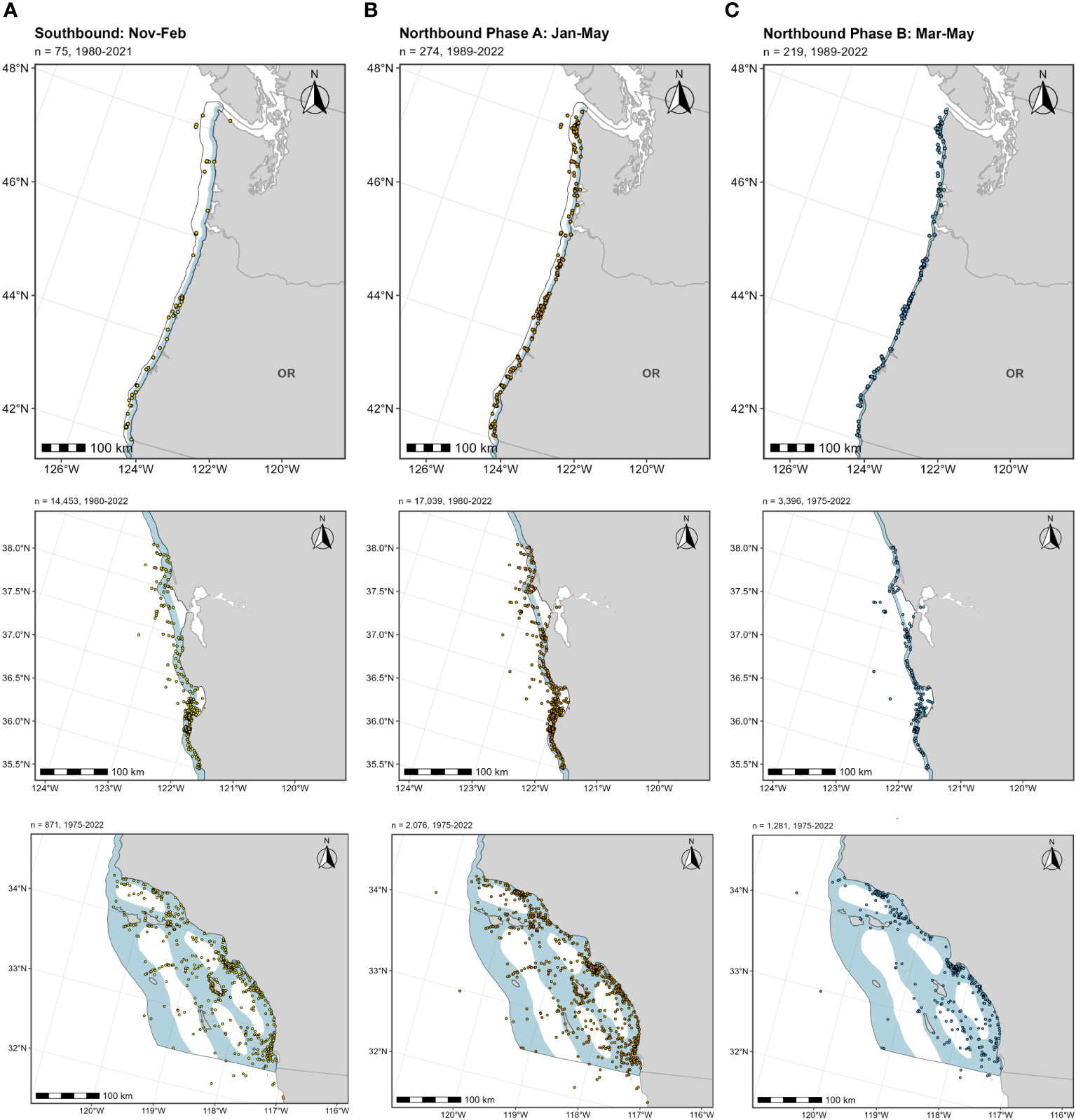
Figure 9 OBIS-SEAMAP gray whale sightings during each migratory period (left column, (A) southbound; middle column, (B) northbound phase A; right column, (C) northbound phase B) and each regional area where modifications were made to the existing BIAs (top row: Oregon-Washington coasts; middle row: Gulf of the Farallones and Monterey Bay; bottom row: Southern California Bight). For each migratory period (i.e., column), the previous BIA delineated by Calambokidis et al. (2015) is shown as a light blue shaded polygon, with the revised BIA outlined in black.

3.4.4.2 Parent M-BIA: November-June, transboundary

The parent M-BIA was defined as the revised southbound BIA (see details below) merged with an extension north along the west coast of British Columbia and up to the southernmost extent of the Gulf of Alaska ENP gray whale migratory BIA (see Wild et al., 2023) to explicitly define the migratory connectivity between these two regions (Figure 10); as such, this parent BIA represents a transboundary BIA. This transboundary extension roughly follows the continental shelf off of Vancouver Island and along the west coast of Haida Gwaii, encompassing the inside waters of Haida Gwaii which migrating gray whales have been known to use (Ford et al., 2013; Lagerquist et al., 2019; Urbán R et al., 2021). Lastly, we defined the time period of this BIA as November through June to capture both northbound and southbound migrations from southeast Alaska to southern California (Pike, 1962; Herzing and Mate, 1984; Poole, 1984; Shelden et al., 2000; Rugh et al., 2001; Mate and Urban-Ramirez, 2003; Urbán R et al., 2021).

Figure 10

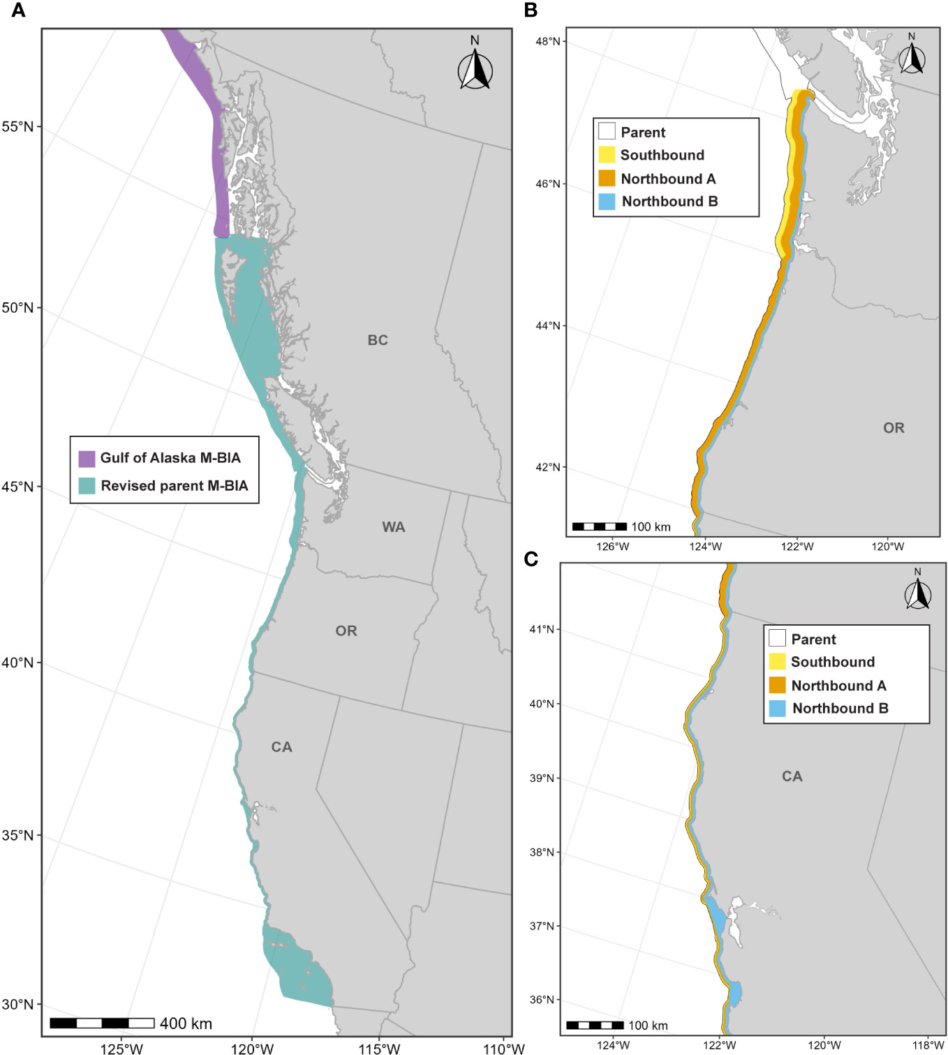
Figure 10 Revised M-BIAs for gray whales along the U.S. West Coast. (A) revised parent BIA (teal polygon) spanning both northbound and southbound migrations between November through June and Gulf of Alaska M-BIA for gray whales (Ferguson et al., 2015; Wild et al., 2023; purple polygon); (B) revised child BIAs (southbound, northbound phase A, northbound phase B) along the Oregon and Washington coasts, where migratory corridors were expanded offshore; (C) revised child BIAs along the central to northern California coast, showing expansion into Monterey Bay and the Gulf of the Farallones. Note: all gray whale migratory BIA boundaries here share the same area in the Southern California Bight, as shown in the left panel. Distance from shore delineations for the remainder of the migration route are as follows: central-northern California coast (parent & southbound: 10-km; northbound phase A: 8-km, northbound phase B: 5-km); Oregon (parent & southbound: 15-km; northbound phase A: 15-km; northbound phase B: 5-km); Washington (parent & southbound: 30-km; northbound phase A: 20-km; northbound phase B: 5-km).

3.4.4.3 Southbound BIA: November-February

The southbound M-BIA boundary delineated by Calambokidis et al. (2015) was defined as a corridor extending 10 km from shore along the entire West Coast. While this corridor width may be reasonable for southbound migrating gray whales along northern and central California (Shelden and Laake, 2002; OSU, Unpublished), there is evidence for a broader, more offshore distribution with increasing latitude along the West Coast region (Table 2). For example, off the Oregon coast southbound migrating gray whales have been documented as far as 23 km from shore during aerial surveys and were on average 12 km from shore (Green et al., 1995). Even farther offshore distributions of southbound migrating gray whales have been reported along the Washington coast; during aerial surveys, gray whales were on average 24 km from shore with a maximum distance from shore of 43 km (Green et al., 1995). Early logbook reports from offshore lightships included a sighting off Cape Flattery that was 32 km from shore (Pike, 1962). Visual surveys undertaken by CRC off the Washington coast support a similar distribution of southbound migrating gray whales, with nearly all sightings between 10-30 km from shore (maximum = 57 km; CRC Unpublished). OBIS-SEAMAP sightings in this region also support this distribution (Figure 9; Halpin et al., 2009). Based on these lines of evidence, it was deemed appropriate to redefine the southbound migratory corridor along the Oregon coast to 15 km wide and the portion along the Washington coast to 30 km (Figure 10). Lastly, the time period of the southbound BIA was redefined as the period spanning November through February (previously October through March) to capture the majority of southbound migrating gray whales along the U.S. West Coast region (Pike, 1962; Shelden et al., 2000; Rugh et al., 2001).

3.4.4.4 Northbound phase A BIA: January-May

The northbound phase A M-BIA (primarily adults and juveniles) described by Calambokidis et al. (2015) was defined as a corridor of 8 km from shore uniformly along the U.S. West Coast. The 8 km distance from shore delineation is appropriate for the region north of the SCB through the remainder of California (Shelden and Laake, 2002; OSU, Unpublished; Poole, 1984; Carretta and Forney, 1993; Mate and Urban-Ramirez, 2003). Both aerial surveys and locations from satellite tagged ENP gray whales indicate a slightly broader distribution off the Oregon coast (Table 2; Green et al., 1995; OSU, Unpublished). Off the Washington coast northbound migrating gray whales have been documented just over 25 km from shore (Washington Department of Fisheries and Wildlife (WDFW) pers comm, 2022; Green et al., 1995; OSU, Unpublished; CRC, Unpublished). Based on these lines of evidence supporting variation in migratory corridor width with increasing latitude, we revised the northbound phase A BIA by expanding the corridor to 15 km from shore off the Oregon coast and 20 km from shore off the Washington coast (Figure 10). Lastly, the time period of this BIA was redefined as the period spanning January through May (previously January-July) to capture the vast majority of northbound (phase A) migrating gray whales within the U.S. West Coast region (Poole, 1984; Rugh et al., 2001).

3.4.4.5 Northbound phase B BIA: March-May

The northbound phase B BIA (primarily cow/calf pairs) described by Calambokidis et al. (2015) remained largely the same (5 km from shore corridor along the entire coast north of the SCB) with exception of the modifications that were applied to all migratory BIAs described herein (i.e., encompassing Monterey Bay, Gulf of Farallones, SCB). A number of previous studies support the nearshore corridor for northbound migrating gray whales consisting heavily of cows and calves (Table 3; Herzing and Mate, 1984; Poole, 1984; Halpin et al., 2009; WDFW pers comm, 2022) and so this zone is also treated as an R-BIA due to this heavy use by mothers and dependent calves consistent with the definition for Reproductive BIAs (Harrison et al., 2023). While this BIA previously spanned months March through July, we redefined the time period for this corridor to March through May to more accurately reflect the time period that this phase of gray whales occurs on the U.S. West Coast, rather than that of their entire northbound migratory route to the Arctic (Poole, 1984). This BIA is totally within the Phase A BIA but reflects the narrower corridor and more specific time period for the mother and calf portion of the migration.

3.4.4.6 Note on WNP gray whales

Although there is documentation of two satellite tagged WNP gray whales using part of the migratory corridor described by the BIAs delineated here (Mate et al., 2015) – with one WNP whale using a large portion of the route – these BIAs intend to capture important migratory routes for ENP gray whales as understanding of ENP gray whale use of the U.S. West Coast for this purpose is much more comprehensive than what is currently known for WNP gray whales. Therefore, while it is important to note that WNP gray whales may use the migratory corridors reflected in these BIAs, there is limited evidence to fully extend these BIAs to the WNP gray whale population and thus our BIAs and associated scores are centered on the ENP gray whale population and migrating PCFG gray whales.

3.4.4.7 Scoring

Scores for the gray whale M-BIAs and the one R-BIA are listed in Table 1 and were informed by the width, duration (time period), and the proportion of the population and demographics captured by each BIA. As such, higher scores (e.g., Importance, Intensity) were associated with narrower corridors, shorter migratory periods, migratory periods for vulnerable demographics (i.e., mom/calf pairs), and migratory BIAs with strong, comprehensive lines of supporting evidence. Full scoring narratives are provided in Supplementary Materials and on the BIA website.

3.5 Southern resident killer whale S-BIA

3.5.1 Background

The SRKWs are a demographically distinct transboundary population of killer whales in the eastern North Pacific, comprised of three matrilineal pods (J, K and L). Annual censuses undertaken by the Center for Whale Research (CWR) since 1976 have documented long-term population trends and occurrence in the Salish Sea (inland waters). SRKW abundance was reduced in the 1960s-70s due to live capture for marine parks, slowly increased through the mid-1990s (peaked 1995 at 98 individuals) and has since declined to 73 individuals as of July 2022 (Center for Whale Research (CWR), 2022). The population was first listed as Threatened in Canada in 1999 and then Endangered in 2001 (Baird, 2001), while in the U.S., SRKWs were listed as Endangered under the Endangered Species Act in 2005. Threats to the long-term viability of SRKWs include reduced quantity and quality of prey, exposure to persistent organic pollutants, disturbance from vessels, and small population size (Krahn et al., 2004; 2009; Ford et al., 2010; Wasser et al., 2017; Hanson et al., 2021; Holt et al., 2021; Kardos et al., 2023).

The SRKWs are periodically present in the protected waters of the Salish Sea, particularly during early spring, summer, and fall months, with evidence for varying pod-specific core areas of use (Ford et al., 2000; Hauser et al., 2007; Olson et al., 2018). While less is known about their distribution during the winter and early spring, sighting, satellite tagging, and passive acoustic studies have documented their occurrence on the outer coasts of British Columbia, Washington, Oregon, and California during these seasons (Hanson et al., 2013; Emmons et al., 2021; 2018). However, SRKW’s presence in the Salish Sea has noticeably declined – and timing of presence shifted – over recent years; it is suspected that these whales are spending their time in other areas within their range, such as the outer coast (Shields et al., 2018; Hanson et al., 2021; Ettinger et al., 2022). This population feeds exclusively on fish, with Chinook salmon (Oncorhynchus tshawytscha) representing a large proportion of their diet throughout the year, despite known variability in their seasonal distribution and the fact that many Chinook salmon stocks they feed on are Endangered or Threatened themselves (Hanson et al., 2021).

Here we delineated an S-BIA for the SRKW population for the U.S. West Coast region, which was not previously designated in Calambokidis et al. (2015). While there have been some records of SRKW occurrence in waters as far north as southeast Alaska, for this assessment we focused on the extent of their known range within the West Coast region and incorporated identified important areas in adjacent Canadian waters of the Salish Sea. For the parent BIA, we used existing spatial boundaries that have been well justified through current understanding of their distribution: the U.S. NMFS Critical Habitat boundary and the Fisheries and Oceans Canada (DFO) Critical Habitat boundary. We further identified core areas of use (core BIAs) using information on their movements obtained from satellite tracking data and a core area in the Salish Sea previously identified as NOAA Critical Habitat.

3.5.2 BIA boundary delineation and scoring

The basis for the parent BIA for SRKWs was a combination of the Critical Habitat boundaries defined by NOAA Fisheries (U.S. waters) and DFO Canada (Fisheries and Oceans Canada, 2011; NMFS, 2021). Both Critical Habitat boundaries reflect areas within the geographical range of SRKWs that contained physical and/or biological features important to their survival. In August 2021, NOAA Fisheries revised the Critical Habitat for this population by extending the boundary from the Strait of Juan de Fuca to include outer coast waters (between 6- and 200-m isobaths) with Point Sur, California, representing the southernmost extent (NMFS, 2021). While Critical Habitat excluded the Quinault Military Range Site off the Washington coast, since BIAs are based solely on biological criteria, we include the portion of the range that was deemed biologically important for SRKWs. The parent BIA was drawn by combining Critical Habitat boundaries from both NOAA Fisheries and DFO. The resulting range size of the parent BIA is 60,348 km² (Figure 11).

Figure 11

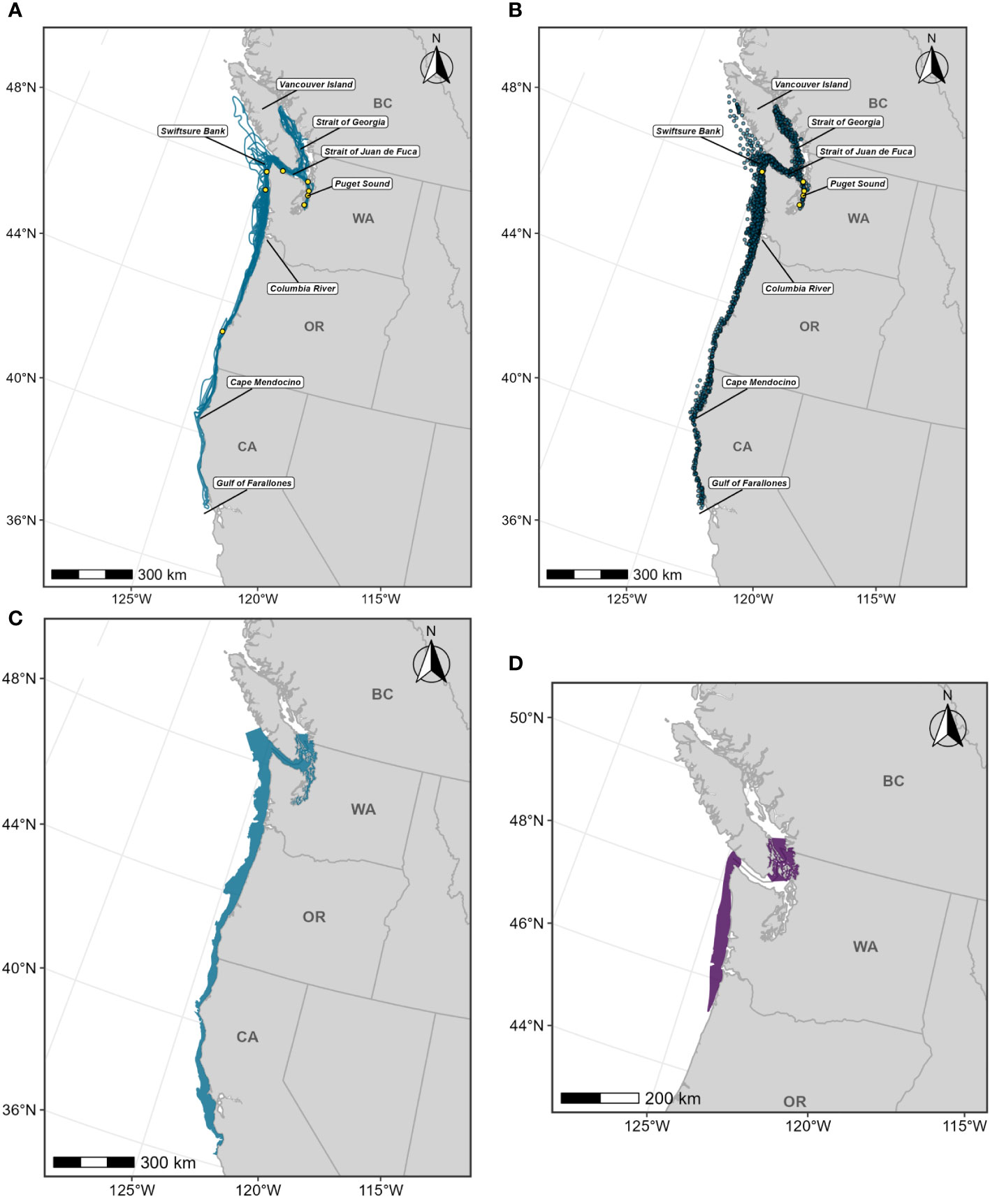
Figure 11 Top panel: (A) Crawl tracks (blue lines) of all satellite tagged Southern Resident killer whales (n=8; 2012-2016; Supplementary Table 3) with deployment locations shown as green circles (B) 4-hour crawl locations of Southern Resident killer whale tracks used in kernel density analysis (n=5) with deployment locations shown as green circles). All crawl-derived locations were re-routed to avoid tracks crossing land. Bottom panel: (C) Parent BIA for Southern Resident killer whales represented as both NOAA and DFO critical habitat boundaries (WA Quinault Range included). The resulting area size is 60,348 km²; (D) Child BIA representing the core range of Southern Resident killer whales, based off of NOAA Fisheries critical habitat core range and a 50% isopleth of UD estimated from kernel density analysis on satellite tag data (total area = 14,809 km²).

A core BIA was delineated for SRKWs with the intent of highlighting areas of intensified use within their overall range. The basis of the core BIA was a combination of NOAA’s Critical Habitat core area (around the San Juan Islands, extended across the U.S./Canada border) and high-density areas identified through kernel density analyses of satellite tag data (details on satellite tag data methods are described in Supplementary File A, Section S2.3 and follow those used by the Hawai’i region (Kratofil et al., 2023; Figure 11). While NOAA’s Critical Habitat core range is designated as a “summer core range”, SRKW occurrence in this region during summer months has declined considerably over recent years; the importance of this area for SRKWs may not be as strongly associated with this particular season as has been the case historically (Shields et al., 2018; Hanson et al., 2021; Ettinger et al., 2022). As such, we specify the core BIA described here to exist year-round for SRKWs.

Scores for the SRKW S-BIA are provided in Table 1 and comprehensive narratives are provided in Supplementary Materials and on the BIA website. The Intensity score for the parent BIA was derived through the quantitative S-BIA scoring matrix, which combines abundance (73 individuals) and range size of the BIA (60,348 km²). The S-BIA scoring matrix is not used for the core BIA. Because the core BIA for this population represents intensified use relative to the broader parent BIA, it was appropriate to score the core BIA with the highest Intensity score. We highlight particular attention to the Data Support and Boundary Certainty scores for this BIA (parent = 3, core = 2 for each score type). Long-term photo-identification and continuous monitoring efforts support the exact abundance value of 73 individuals (Center for Whale Research (CWR), 2022). Areas within the core BIA align with those of known concentrated use based on external studies, such as sightings (Hauser et al., 2007; Olson et al., 2018) and acoustic detections (Hanson et al., 2013; 2018; Emmons et al., 2021). The parent BIA and a portion of the core BIA (San Juan Islands region) were based on published Critical Habitat boundaries in both U.S. and adjacent Canadian waters, which encompass the known extent of SRKWs within the U.S. West Coast region and incorporate habitat features known to be important to this population’s survival. Important areas in the Salish Sea are primarily supported by over 30 years of sighting data (Olson et al., 2018). Although the majority of these data capture only a portion of their range (Salish Sea), limited SRKW sightings along the outer coast where there is extensive community scientist effort (e.g., whale watching operations in Monterey Bay) may reflect that it is very unlikely that the SRKWs spend a lot of their time in areas farther south within the West Coast region. Important areas along the outer coast are supported by movements from eight satellite tagged SRKWs, from all three pods (3-95 days of data; Supplementary Table 3), which complement our understanding of their use outside of the Salish Sea and provide a less biased (compared to dedicated survey effort) depiction of their habitat use in areas that are often inaccessible for surveys due to poor working conditions. The importance of this area has been more recently supported through passive acoustic studies (Emmons et al., 2021). The outer coast core area also includes the mouths of river systems that play a large role in supporting prey for SRKWs (e.g., Columbia River; Zamon et al., 2007; Hanson et al., 2021). The methods used to derive the core areas from satellite tag data are widely used, robust, and accounted for varying deployment durations. Despite these various strengths, sightings in typical high-use areas have declined over recent years (Shields et al., 2018; Hanson et al., 2021), adding uncertainty to a contemporary understanding of SRKW distribution, particularly their core areas. Collectively, heterogeneous data support (including strengths/weaknesses and types) throughout the SRKW’s range and uncertainty related to recent changes in their distribution drove the scores for the parent and child SRKW S-BIAs.

3.6 Harbor porpoise S-BIAs

3.6.1 Background

Harbor porpoise occur widely in coastal nearshore and inland waters along the U.S. West Coast (Gaskin, 1984). Their nearshore distribution has made them vulnerable to human activities, especially entanglements in gillnet fisheries (Gaskin, 1984). Two S-BIAs were developed for harbor porpoise previously (Calambokidis et al., 2015) and for this assessment we have kept these unchanged as there have been no additional lines of evidence to suggest a need for modifying existing boundaries since 2015.

3.6.2 BIA boundary delineation and scoring

Calambokidis et al. (2015) delineated two small and resident BIAs for harbor porpoise off the West Coast based on recognized stock boundaries for the Monterey Bay and Morro Bay regions and the BIAs here are taken directly from those boundaries. Several lines of evidence suggest these separate populations have a restricted range, including regional differences in contaminant concentrations and ratios (Calambokidis and Barlow, 1991), genetic studies (Chivers et al., 2002; 2007; Morin et al., 2021), and densities derived from aerial and ship surveys (Forney et al., 1991; 2021; Forney, 1995; 1999; Carretta et al., 2001; 2009). Boundaries were defined using the approximate 200-m isobath from land for each stock boundary (Morro Bay = Point Conception to Point Sur; Monterey Bay = Point Sur to Pigeon Point). In this assessment we used the same boundaries to represent these two BIAs (Figure 12).

Figure 12

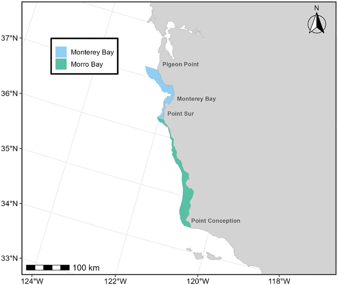
Figure 12 Monterey Bay and Morro Bay harbor porpoise S-BIAs for the U.S. West Coast region. Harbor porpoise BIAs shown here were delineated by Calambokidis et al. (2015) and were not revised for this assessment. BIA boundaries are based on stock boundaries for each stock/BIA.

Although the spatial boundaries for these two harbor porpoise S-BIAs remained the same, information from previous and more recent studies were used to support the scoring (Table 1; Supplementary Materials). Contemporary abundance estimates from each respective stock assessment report (Carretta et al., 2022) were used in combination with the area of the BIA to determine the Intensity scores through the S-BIA scoring matrix.

4 Other potential areas and species for future consideration

4.1 Cuvier’s beaked whales

No watch list areas were formally designated for the West Coast region in this assessment, but we initially considered developing a BIA for Cuvier’s beaked whales. Accurate information on the distribution and abundance of this species has been limited due to their cryptic nature and occurrence primarily in deep offshore waters making it hard to define its habitat preference across the entire region. This species has been documented as sensitive to anthropogenic disturbance, in particular Navy Sonar (e.g. DeRuiter et al., 2013; Falcone et al., 2017). Recently, however, additional information and approaches are providing a better picture of this species off the U.S. West Coast (Curtis et al., 2021; Barlow et al., 2021a; 2021b, Schorr et al., 2014; Bernaldo de Quirós et al., 2019). The development and use of floating drifting hydrophones to supplement the NOAA visual sighting surveys has also provided more complete information on their broader distribution and abundance along the U.S. West Coast (Barlow et al., 2018; 2021a; 2021b; 2022). These new approaches have resulted in a new abundance estimate of Cuvier’s beaked whale off the U.S. West Coast of 5,454 individuals (95% confidence intervals: 3,151 to 8,907). While the species is broadly distributed along the U.S. West Coast, there is increasing evidence using satellite telemetry suggesting there may be small discrete populations which have high site fidelity over long time periods (e.g. Schorr et al., 2014; 2022a; 2022b). In addition, the development of mark-recapture abundance models for this species in the San Nicolas Basin in Southern California has provided abundance and preliminary trend data for this region, indicating a localized population estimated at 121 (71-219) individuals (Curtis et al., 2021) with individual sighting histories spanning as long as 15 years (Schorr et al., 2022a). The combination of high site fidelity, mark-recapture studies, and acoustic monitoring indicate some areas, including the San Nicolas Basin appear to have higher densities of beaked whales (Falcone et al., 2009; Barlow et al., 2021a, 2021b; Curtis et al., 2021) and may warrant future consideration as a BIA.

5 Conclusions

Revised BIAs delineated here update those determined previously (Calambokidis et al., 2015) and add BIAs for several species. Where available, we applied additional data and developed a more quantitative analytical approach compared to what was used previously. While in general there was fairly good agreement between the multiple datasets we used, where differences existed, the use of multiple datasets helped to address some of the biases and limitations of any one type of data. We also applied a more quantitative and transparent approach to determine the BIA boundaries. The BIAs delineated here for blue and humpback whales are considerably larger than those identified previously, and more consistent with the approach used in other regions. In addition to identifying larger overall BIAs, we also delineated core higher-density areas as part of the new hierarchical component of the BIA II delineation protocol (Harrison et al., 2023). In total, we identified BIAs for six cetacean species in the West Coast region, including feeding areas for blue, fin, and humpback whales, migratory, feeding and reproductive BIAs for gray whales; and small and resident populations for harbor porpoise and Southern Resident killer whales. These will aid in conservation effort in these most important locations.

Data availability statement

The raw data supporting the conclusions of this article will be made available by the authors, without undue reservation.

Ethics statement

The animal study was approved by Cascadia Research Collective and OSU IACUC. The study was conducted in accordance with the local legislation and institutional requirements.

Author contributions

JC: Conceptualization, Funding acquisition, Investigation, Methodology, Project administration, Supervision, Writing – original draft, Writing – review & editing. MK: Conceptualization, Formal analysis, Investigation, Methodology, Validation, Writing – original draft, Writing – review & editing. DP: Data curation, Investigation, Methodology, Writing – review & editing. BL: Investigation, Methodology, Writing – review & editing. GS: Investigation, Methodology, Writing – review & editing. MH: Investigation, Methodology, Writing – review & editing. RB: Investigation, Methodology, Writing – review & editing. KF: Investigation, Methodology, Writing – review & editing. EB: Investigation, Methodology, Writing – review & editing. RR: Investigation, Methodology, Writing – review & editing. EH: Investigation, Methodology, Writing – review & editing.

Funding

The author(s) declare financial support was received for the research, authorship, and/or publication of this article. NOAA provided support for the current and past efforts to develop the U.S. West Coast BIAs and has supported studies that generated the data used. Funding for CRC fieldwork during which many of the data were collected was received from NOAA, and the U.S. Navy (LMR, ONR, and Pacific Fleet). Funding for OSU’s blue, fin, humpback, and gray whale satellite tagging work was provided by the U.S. Navy’s Office of Naval Research (1995-2000), the Tagging of Pacific Predators (2004-2005), Pacific Life Foundation (2014-2015), Makana Aloha Foundation (2015), the U.S. Navy’s Commander, Pacific Fleet (2009-2019), and private donors to the OSU Marine Mammal Institute Endowment. Funding for MarEcoTel’s fin whale tagging was provided by the U.S. Navy (LMR, Pacific Fleet, and ONR), and NOAA. Sighting data used to develop the habitat-based density models were collected on ship surveys conducted by Southwest Fisheries Science Center and funded by NOAA Fisheries, with the exception of the 2018 survey that was conducted as part of the Pacific Marine Assessment Program for Protected Species (PacMAPPS), a collaborative effort between NOAA Fisheries, the U.S. Navy, and BOEM (BOEM funding was provided via Interagency Agreement (IAA) M17PG00025, and Navy funding via IAA N0007018MP4C560).

Acknowledgments

Information used in the BIAs delineations reported here came from a wide variety of sources and approaches. Sighting and behavioral data in the CRC sighting database came from many contributors and researchers who have participated in conducting this work over the years and compiling and processing this data; we particularly thank Kiirsten Flynn, James Fahlbusch, Alex Vanderzee, Jack Barkowski, Elana Dobson, Alie Perez, Ian Flynn-Thomas, and many others. Work by CRC, OSU, NOAA (SWFSC, NWFSC), and MarEcoTel were conducted under permits from NMFS for both the survey and tagging efforts. Contributions to the SWFSC line-transect surveys are included in Becker et al. (2020b). We thank Sheila Thornton for providing the DFO Southern Resident Killer Whale Critical Habitat shapefiles. Scott Pearson of WDFW provided data about gray whale sightings from their surveys off Washington. We appreciate Ei Fujioka, and Sarah DeLand, for their assistance with the BIA description tool website and for compiling BIA metadata and Lauren Wild for discussions on gray whale migratory corridors. We thank Jolie Harrison, Sofie Van Parijs, Megan Ferguson, Reny Tyson-Moore, and other reviewers for feedback on early versions of the manuscript. Simone Baumann-Pickering and Jay Barlow provided important insights on beaked whale acoustic detections. We thank reviewer(s) with the U.S. Navy, and two additional reviewers, who made numerous helpful comments.

Conflict of interest

EB was employed by Ocean Associates, Inc.

The remaining authors declare that the research was conducted in the absence of any commercial or financial relationships that could be construed as a potential conflict of interest.

Publisher’s note

All claims expressed in this article are solely those of the authors and do not necessarily represent those of their affiliated organizations, or those of the publisher, the editors and the reviewers. Any product that may be evaluated in this article, or claim that may be made by its manufacturer, is not guaranteed or endorsed by the publisher.

Author disclaimer

The views expressed here are those of the authors and do not necessarily reflect the views of the U.S. National Marine Fisheries Service, NOAA.

Supplementary material

The Supplementary Material for this article can be found online at: https://www.frontiersin.org/articles/10.3389/fmars.2024.1283231/full#supplementary-material

Footnotes

1. ^ https://oceannoise.noaa.gove/biologically-important-areas.
2. ^ https://seamap.env.duke.edu/.

References

Abrahms B., Hazen E. L., Aikens E. O., Savoca M. S., Goldbogen J. A., Bograd S. J., et al. (2019b). Memory and resource tracking drive blue whale migrations. Proc. Natl. Acad. Sci. 116, 5582–5587. doi: 10.1073/pnas.1819031116

CrossRef Full Text | Google Scholar

Abrahms B., Welch H., Brodie S., Jacox M. G., Becker E. A., Bograd S. J., et al. (2019a). Dynamic ensemble models to predict distributions and anthropogenic risk exposure for highly mobile species. Divers. Distrib. 25, 1182–1193. doi: 10.1111/ddi.12940

CrossRef Full Text | Google Scholar

Archer F. I., Brownell R. L. Jr., Hancock-Hanser B. L., Morin P. A., Robertson K. M., Sherman K. K., et al. (2019). Revision of fin whale Balaenoptera physalus (Linnaeus 1758) subspecies using genetics. J. Mammal. 100, 1653–1670. doi: 10.1093/jmammal/gyz121

CrossRef Full Text | Google Scholar

Archer F. I., Morin P. A., Hancock-Hanser B. L., Robertson K. M., Leslie M. S., Bérubé M., et al. (2013). Mitogenomic phylogenetics of fin whales (Balaenoptera physalus spp.): genetic evidence for revision of subspecies. PLoS One 8, e63396. doi: 10.1371/journal.pone.0063396

PubMed Abstract | CrossRef Full Text | Google Scholar

Bailey H., Mate B. R., Palacios D. M., Irvine L., Bograd S. J., Costa D. P. (2009). Behavioural estimation of blue whale movements in the Northeast Pacific from state-space model analysis of satellite tracks. Endanger. Species Res. 10, 93–106. doi: 10.3354/esr00239

CrossRef Full Text | Google Scholar

Baird R. W. (2001). Status of killer whales, Orcinus orca, in Canada. Can. Field Nat. 115, 676–701. doi: 10.5962/p.363865

CrossRef Full Text | Google Scholar

Baker C. S., Steel D., Calambokidis J., Barlow J., Burdin A. M., Clapham P. J., et al. (2008). geneSPLASH: An initial, ocean-wide survey of mitochondrial (mt) DNA diversity and population structure among humpback whales in the North Pacific (National Fish and Wildlife Foundation).

Google Scholar

Baker C. S., Steel D., Calambokidis J., Falcone E., Gonzalez-Peral U., Barlow J., et al. (2013). Strong maternal fidelity and natal philopatry shape genetic structure in North Pacific humpback whales. Mar. Ecol. Prog. Ser. 494, 291–306. doi: 10.3354/meps10508

CrossRef Full Text | Google Scholar

Barlow J. (2016). Cetacean abundance in the California Current estimated from ship-based line-transect surveys in 1991-2014 (La Jolla, CA, USA: NOAA Southwest Fisheries Science Center Administrative Report LJ-16-01). 63p.

Google Scholar

Barlow J., Calambokidis J., Falcone E. A., Baker C. S., Burdin A. M., Clapham P. J., et al. (2011). Humpback whale abundance in the North Pacific estimated by photographic capture-recapture with bias correction from simulation studies. Mar. Mamm. Sci. 27, 793–818. doi: 10.1111/j.1748-7692.2010.00444.x

CrossRef Full Text | Google Scholar

Barlow J., Forney K. A. (2007). Abundance and population density of cetaceans in the California Current ecosystem. Fishery Bull. 105, 509–526.

Google Scholar

Barlow J., Fregosi S., Thomas L., Harris D., Griffiths E. T. (2021a). Acoustic detection range and population density of Cuvier's beaked whales estimated from near-surface hydrophones. J. Acoust. Soc Am. 149, 111–125. doi: 10.1121/10.0002881

PubMed Abstract | CrossRef Full Text | Google Scholar

Barlow J., Griffiths E. T., Klinck H., Harris D. V. (2018). Diving behavior of Cuvier's beaked whales inferred from three-dimensional acoustic localization and tracking using a nested array of drifting hydrophone recorders. J. Acoust. Soc Am. 144, 2030–2041. doi: 10.1121/1.5055216

PubMed Abstract | CrossRef Full Text | Google Scholar

Barlow J., Moore J. E., McCullough J. L., Griffiths E. T. (2022). Acoustic-based estimates of Cuvier's beaked whale (Ziphius cavirostris) density and abundance along the U.S. West Coast from drifting hydrophone recorders. Mar. Mamm. Sci. 38, 517–538. doi: 10.1111/mms.12872

CrossRef Full Text | Google Scholar

Barlow J., Trickey J. S., Schorr G. S., Moore J. E. (2021b). Recommended snapshot length for acoustic point-transect surveys of intermittently available beaked whales. J. Acoust. Soc Am. 149, 3830–3840. doi: 10.1121/10.0005108

PubMed Abstract | CrossRef Full Text | Google Scholar

Becker E. A., Caretta J. V., Forney K. A., Barlow J., Brodie S., Hoopes R., et al. (2020a). Performance evaluation of cetacean species distribution models developed using generalized additive models and boosted regression trees. Ecol. Evol. 10, 5759–5784. doi: 10.1001/ece3.6316

PubMed Abstract | CrossRef Full Text | Google Scholar

Becker E. A., Forney K. A., Ferguson M. C., Barlow J., Redfern J. V. (2012). “Predictive modeling of cetacean densities in the California Current ecosystem based on summer/fall ship surveys in 1991-2008,” NOAA Technical Memorandum, NOAA-TM-NMFS-SWFSC ; 499 (Southwest Fisheries Science Center, National Oceanographic and Atmospheric Administration, La Jolla, CA).

Google Scholar

Becker E. A., Forney K. A., Miller D. L., Fiedler P. C., Barlow J., Moore J. E. (2020b). “Habitat-based density estimates for cetaceans in the California Current Ecosystem based on 1991-2018 survey data,” NOAA Technical Memorandum, NMFS-SWFSC-638 (Southwest Fisheries Science Center, National Oceanic and Atmospheric Administration, La Jolla, CA).

Google Scholar

Becker E. A., Forney K. A., Thayre B. J., Debich A., Campbell G. S., Whitaker K., et al. (2017). Habitat-based density models for three cetacean species off Southern California illustrate pronounced seasonal differences. Front. Mar. Sci. 4, 1–14. doi: 10.3389/fmars.2017.00121

CrossRef Full Text | Google Scholar

Berman-Kowalewski M., Gulland M. D., Wilkin S., Calambokidis J., Mate B., Cordaro J., et al. (2010). Association Between Blue Whale (Balaenoptera musculus) Mortality and Ship Strikes Along the California Coast. Aquat. Mamm 36 (1), 59–66. doi: 10.1578/AM.36.1.2010.59

CrossRef Full Text | Google Scholar

Bernaldo de Quir´s Y., Fernandez A., Baird R. W., Brownell R. L., Aguilar de Soto N., Allen D., et al. (2019). Advances in research on the impacts of anti-submarine sonar on beaked whales. Proc. R. Soc B 286, 20182533. doi: 10.1098/rspb.2018.2533

CrossRef Full Text | Google Scholar

Bettridge S. O. M., Baker C. S., Barlow J., Clapham P., Ford M. J., Gouveia D., et al. (2015). “Status review of the humpback whale (Megaptera novaeangliae) under the Endangered Species Act,” NOAA Technical Memorandum, NOAA-TM-NMFS-SWFSC-540 (Southwest Fisheries Science Center, National Oceanic and Atmospheric Administration, La Jolla, CA).

Google Scholar

Calambokidis J. (2016). Study of seasonal resident gray whales feeding strategy in N Puget Sound, WA in 2016 (Contract Report for Cooperative Agreement CA-16-320 to Washington Department of Natural Resources).

Google Scholar

Calambokidis J., Barlow J. (1991). Chlorinated hydrocarbon concentrations and their use for describing population discreteness in harbor porpoises from Washington, Oregon, and California. Eds. Reynolds J. E. III, Odell D. K. (Marine mammal strandings in the United States. NOAA Technical Report NMFS 98), 101–110.

Google Scholar

Calambokidis J., Barlow J. (2004). Abundance of blue and humpback whales in the eastern North Pacific estimated by capture-recapture and line-transect methods. Mar. Mamm. Sci. 20, 63–85. doi: 10.1111/j.1748-7692.2004.tb01141.x

CrossRef Full Text | Google Scholar

Calambokidis J., Barlow J. (2013). Updated abundance estimates of blue and humpback whales off the US West Coast incorporating photo-identifications from 2010 and 2011 (U.S. Department of Commerce). PSRG-2013-13R

Google Scholar

Calambokidis J., Barlow J. (2020). “Abundance estimates for blue and humpback whales along the U.S. West Coast using data through 2018,” NOAA Technical Memorandum, NMFS-SWFSC-634 (Southwest Fisheries Science Center, National Oceanographic and Atmospheric Administration, La Jolla, CA).

Google Scholar

Calambokidis J., Barlow J., Flynn K., Dobson E., Steiger G. H. (2017). Update on abundance, trends, and migrations of humpback whales along the US West Coast (Seattle WA: IWC Report SC/A17/NP/13 for the Workshop on the Comprehensive Assessment of North Pacific Humpback Whales).

Google Scholar

Calambokidis J., Barlow J., Ford J. K. B., Chandler T. E., Douglas A. B. (2009). Insights into the population structure of blue whales in the eastern North Pacific from recent sightings and photographic identifications. Mar. Mamm. Sci. 25, 816–832. doi: 10.1111/j.1748-7692.2009.00298.x

CrossRef Full Text | Google Scholar

Calambokidis J., Darling J. D., Deecke V., Gearin P., Gosho M., Megill W., et al. (2002). Abundance, range and movements of a feeding aggregation of gray whales (Eschrichtius robustus) from California to southeastern Alaska in 1998. J. Cetacean Res. Manage. 4, 267–276. doi: 10.47536/jcrm.v4i3.839

CrossRef Full Text | Google Scholar

Calambokidis J., Evenson J. R., Chandler T. E., Steiger G. H. (1992). Individual identification of gray whales in Puget Sound in 1991. Puget Sound Notes 28, 1–4.

Google Scholar

Calambokidis J., Fahlbusch J. A., Szesciorka A. R., Southall B. L., Cade D. E., Friedlaender A. S., et al. (2019a). Differential vulnerability to ship strikes between day and night for blue, fin, and humpback whales based on dive and movement data from medium duration archival tags. Front. Mar. Sci. 6. doi: 10.3389/fmars.2019.00543

CrossRef Full Text | Google Scholar

Calambokidis J., Falcone E. A., Quinn T. J., Burdin A. M., Clapham P. J., Ford J. K. B., et al. (2008). SPLASH: Structure of Populations, Levels of Abundance and Status of Humpback Whales in the North Pacific (Seattle, Washington, USA: Final report for Contract AB133F-03-RP-00078 prepared by Cascadia Research for U.S. Department of Commerce). Available at: http://www.cascadiaresearch.org/SPLASH/SPLASH-contract-Report-May08.pdf.

Google Scholar

Calambokidis J., Laake J. L., Klimek A. (2010). Abundance and population structure of seasonal gray whales in the Pacific Northwest 1998-2008 (IWC Report SC/62/BRG32 submitted to IWC Scientific Committee). 50 pp.

Google Scholar

Calambokidis J., Laake J., Perez A. (2014). Updated analysis of abundance and population structure of seasonal gray whales in the Pacific Northwest 1996-2012 (Seattle, WA: Final Report to National Marine Mammal Laboratory).

Google Scholar

Calambokidis J., Perez A., Laake J. (2019b). Updated analysis of abundance and population structure of seasonal gray whales in the Pacific Northwest 1996-2017 (Seattle, WA: Final Report to NOAA).

Google Scholar

Calambokidis J., Steiger G. H., Cubbage J. C., Balcomb K. C., Ewald C., Kruse S., et al. (1990). Sightings and movements of blue whales off central California 1986-88 from photo identification of individuals. Rep. Int. Whal. Commn. (special issue 12), 343–348.

Google Scholar

Calambokidis J., Steiger G. H., Curtice C., Harrison J., Ferguson M. C., Becker E., et al. (2015). Biologically dE selected cetaceans within U.S. Waters – west coast region. Aquat. Mamm. 41, 39–53. doi: 10.1578/AM.41.1.2015.39

CrossRef Full Text | Google Scholar

Calambokidis J., Steiger G. H., Ellifrit D. K., Troutman B. L., Bowlby C. E. (2004). Distribution and abundance of humpback whales and other marine mammals off the northern Washington coast. Fish. Bull. 102, 563–580.

Google Scholar

Calambokidis J., Steiger G. H., Evenson J. R., Flynn K. R., Balcomb K. C., Claridge D. E., et al. (1996). Interchange and isolation of humpback whales off California and other North Pacific feeding grounds. Mar. Mamm. Sci. 12, 215–226. doi: 10.1111/j.1748-7692.1996.tb00572.x

CrossRef Full Text | Google Scholar

Calambokidis J., Steiger G. H., Rasmussen K., Urban R. J., Balcomb K. C., Ladron de Guevara P. P., et al. (2000). Migratory destinations of humpback whales that feed off California, Oregon and Washington. Mar. Ecol. Prog. Ser. 192, 295–304. doi: 10.3354/meps192295

CrossRef Full Text | Google Scholar

Calambokidis J., Steiger G. H., Straley J. M., Herman L. M., Cerchio S., Salden D. R., et al. (2001). Movements and population structure of humpback whales in the North Pacific. Mar. Mamm. Sci. 17, 769–794. doi: 10.1111/j.1748-7692.2001.tb01298.x

CrossRef Full Text | Google Scholar

Campbell G. S., Thomas L., Whitaker K., Douglas A. B., Calambokidis J., Hildebrand J. A. (2015). Inter-annual and seasonal trends in cetacean distribution, density and abundance off Southern California. Deep Sea Res. 2. 112, 143–157. doi: 10.1016/j.dsr2.2014.10.008

CrossRef Full Text | Google Scholar

Carretta J. V., Forney K. A. (1993). “Report of the two aerial surveys for marine mammals in California coastal waters utilizing a NOAA DeHavilland Twin Otter Aircraft March 9-April 7, 1991 and February 8-April 6, 1992,” NOAA Technical Memorandum, NMFS NOAA-TM-NMFS-SWFSC-195 (Southwest Fisheries Science Center, National Oceanic and Atmospheric Administration, La Jolla, CA).

Google Scholar

Carretta J. V., Forney K. A., Benson S. R. (2009). “Preliminary estimates of harbor porpoise abundance in California waters from 2002 to 2007,” NOAA Technical Memorandum, NOAA-TM-NMFSSWFSC-435 (Southwest Fisheries Science Center, National Oceanic and Atmospheric Administration, La Jolla, CA).

Google Scholar

Carretta J. V., Oleson E. M., Forney K. A., Muto M. M., Weller D. W., Lang A. R., et al. (2022). “US Pacific marine mammal stock assessments: 2021,” NOAA Technical Memorandum, NOAA-TM-NMFS-SWFSC-663 (Southwest Fisheries Science Center, National Oceanic and Atmospheric Administration, La Jolla, CA).

Google Scholar

Carretta J. V., Taylor B. L., Chivers S. J. (2001). Abundance and depth distribution of harbor porpoise (Phocoena phocoena) in northern California determined from a 1995 ship survey. Fish. Bull. 99, 29–39.

Google Scholar

Center for Whale Research (CWR) (2022). Available at: https://www.whaleresearch.com/ (Accessed 2022).

Google Scholar

Checkley D. M., Barth J. A. (2009). Patterns and processes in the California current system. Progr. Oceanogr. 83, 49–64. doi: 10.1016/j.pocean.2009.07.028

CrossRef Full Text | Google Scholar

Chivers S. J., Dizon A. E., Gearin P. J., Roberston K. M. (2002). Small-scale population structure of eastern North Pacific harbour porpoises, (Phocoena phocoena), indicated by molecular genetic analyses. J. Cetacean Res. Manage. 4, 111–122. doi: 10.47536/jcrm.v4i2.847

CrossRef Full Text | Google Scholar

Chivers S. J., Hanson M. B., Laake J., Gearin P., Muto M. M., Calambokidis J., et al. (2007). Additional genetic evidence for population structure of Phocoena phocoena off the coasts of California, Oregon, and Washington (La Jolla, CA: Southwest Fisheries Science Center, National Oceanic and Atmospheric Administration).

Google Scholar

Curtis K. A., Calambokidis J., Audley K., De Weerdt J., Garita F., Martínez-Loustalot P., et al. (2022). Abundance of humpback whales (Megaptera novaeangliae) wintering in Central America and Southern Mexico from a one-dimensional spatial capture-recapture model (La Jolla, CA: Southwest Fisheries Science Center, National Oceanic and Atmospheric Administration). doi: 10.25923/9cq1-rx80

CrossRef Full Text | Google Scholar

Curtis K. A., Falcone E. A., Schorr G. S., Moore J. E., Moretti D. J., Barlow J., et al. (2021). Abundance, survival, and annual rate of change of Cuvier's beaked whales (Ziphius cavirostris) on a Navy sonar range. Mar. Mamm. Sci. 37, 399–419. doi: 10.1111/mms.12747

CrossRef Full Text | Google Scholar

Darling J. D., Calambokidis J., Balcomb K. C., Bloedel P., Flynn K. R., Mochizuki A., et al. (1996). Movement of a humpback whale (Megaptera novaeangliae) from Japan to British Columbia and return. Mar. Mamm. Sci. 12, 281–287. doi: 10.1111/j.1748-7692.1996.tb00577.x

CrossRef Full Text | Google Scholar

DeRuiter S. L., Southall B. L., Calambokidis J., Zimmer W. M. X., Sadykova D., Falcone E. A., et al. (2013). First direct measurements of behavioural responses by Cuvier's beaked whales to mid-frequency active sonar. Biol. Lett. 9 (4), 20130223. doi: 10.1098/rsbl.2013.0223

PubMed Abstract | CrossRef Full Text | Google Scholar

Derville S., Barlow D. R., Hayslip C., Torres L. G. (2022). Seasonal, annual, and decadal distribution of three rorqual whale species relative to dynamic ocean conditions off Oregon, USA. Front. Mar. Sci. 9. doi: 10.3389/fmars.2022.868566

PubMed Abstract | CrossRef Full Text | Google Scholar

Dohl T. P., Norris K. S., Guess R. C., Bryant J. D., Honig M. W. (1980). “Summary of Marine Mammal and Seabird Surveys of the Southern California Bight Area 1975-1978, Part II: Cetacean of the Southern California Bight,” (U.S. Department of Interior).

Google Scholar

Douglas A. B., Calambokidis J., Munger L. M., Soldevilla M. S., Ferguson M. C., Havron A. M., et al. (2014). Seasonal distribution and abundance of cetaceans off southern California estimated from CalCOFI cruise data from 2004 to 2008. Fish. Bull. 112, 197–220. doi: 10.7755/FB.112.2-3.7

CrossRef Full Text | Google Scholar

Duong T. (2021). Ks: Kernel Smooth. R package version 1.13.2. Available at: https://CRAN.R-project.org/package=ks.

Google Scholar

Emmons C. K., Hanson M. B., Lammers M. O. (2021). Passive acoustic monitoring reveals spatiotemporal segregation of two fish-eating killer whale Orcinus orca populations in proposed critical habitat. Endanger. Species Res. 44, 253–261. doi: 10.3354/esr01099

CrossRef Full Text | Google Scholar

Ettinger A. K., Harvey C. J., Emmons C., Hanson M. B., Ward E. J., Olson J. K., et al. (2022). Shifting phenology of an endangered apex predator mirrors changes in its favored prey. Endanger. Species Res. 48, 211–223. doi: 10.3354/esr01192

CrossRef Full Text | Google Scholar

Falcone E. A., Schorr G. S., Watwood S. L., DeRuiter S. L., Zerbini A. N., Andrews R. D., et al. (2017). Diving behaviour of Cuvier's beaked whales exposed to two types of military sonar. R. Soc Open Sci. 4, 170629. doi: 10.1098/rsos.170629

PubMed Abstract | CrossRef Full Text | Google Scholar

Falcone E. A., Keene E. L., Keen E. M., Barlow J., Stewart J., Cheeseman T., et al. (2022). Movements and residency of fin whales (Balaenoptera physalus) in the California Current System. Mamm. Biol. 102, 1445–1462. doi: 10.1007/s42991-022-00298-4

CrossRef Full Text | Google Scholar

Falcone E. A., Keene E. L., Rone B. K., Schorr G. S. (2018). Distribution and demographics of fin whales in the Southern California Bight (Final report to the US Navy Pacific Fleet Integrated Comprehensive Monitoring Program). Award No. N66604-17-P-2723.

Google Scholar

Falcone E., Schorr G. S., Douglas A., Calambokidis J., Henderson E., McKenna M., et al. (2009). Sighting characteristics and photo-identification of Cuvier's beaked whales (Ziphius cavirostris) near San Clemente Island, California: a key area for beaked whales and the military? Mar. Biol. 156, 2631–2640. doi: 10.1007/s00227-009-1289-8

PubMed Abstract | CrossRef Full Text | Google Scholar

Ferguson M. C., Curtice C., Harrison J. (2015). Biologically Important Areas for cetaceans within U.S. waters - Gulf of Alaska region. Aquat. Mamm. 41 (1), 65–78. doi: 10.1578/AM.411.2015.65

CrossRef Full Text | Google Scholar

Fisheries and Oceans Canada (2011). “Recovery strategy for the Northern and Southern Resident killer whales (Orcinus orca) in Canada,” in Species at Risk Act Recovery Strategy Series (Fisheries & Oceans Canada, Ottawa). Available at: https://www.sararegistry.gc.ca/document/doc1341a/ind_e.cfm. ix + 80 pp.

Google Scholar

Fleming A. H., Clark C. T., Calambokidis J., Barlow J. (2015). Humpback whale diets respond to variance in ocean climate and ecosystem conditions in the California current. Glob. Change Biol. 22, 1214–1224. doi: 10.1111/gcb.13171

CrossRef Full Text | Google Scholar

Ford J. K. B., Durban J. W., Ellis G. M., Towers J. R., Pilkington J. F., Barrett-Lennard L. G., et al. (2013). New insights into the northward migration route of gray whales between Vancouver Island, British Columbia, and southeastern Alaska. Mar. Mamm. Sci. 29, 325–337. doi: 10.1111/j.1748-7692.2012.00572.x

CrossRef Full Text | Google Scholar

Ford J. K. B., Ellis G. M., Balcomb K. C. (2000). Killer whales: The natural history and genealogy of Orcinus orca in British Columbia and Washington (Vancouver: UBC Press).

Google Scholar

Ford J. K. B., Ellis G. M., Olesiuk P. F., Balcomb K. C. (2010). Linking killer whale survival and pre abundance: food limitation in the oceans’ apex predator? Biol. Lett. 6, 139–142. doi: 10.1098/rsbl.2009.0468

PubMed Abstract | CrossRef Full Text | Google Scholar

Forney K. A. (1995). A decline in the abundance of harbor porpoise, Phocoena phocoena, in nearshore waters off California 1986-93. Fish. Bull. 93, 741–748.

Google Scholar

Forney K. A. (1999). The abundance of California harbor porpoise estimated from 1993-97 aerial line transect surveys (La Jolla, CA, USA: Southwest Fisheries Center, National Marine Fisheries Service).

Google Scholar

Forney K. A., Barlow J. (1998). Seasonal patterns in the abundance and distribution of California cetaceans 1991–1992. Mar. Mamm. Sci. 14, 460–489. doi: 10.1111/j.1748-7692.1998.tb00737.x

CrossRef Full Text | Google Scholar

Forney K. A., Ferguson M. C., Becker E. A., Fiedler P. C., Redfern J. V., Barlow J., et al. (2012). Habitat-based spatial models of cetacean density in the eastern Pacific Ocean. Endanger. Species Res. 16, 113–133. doi: 10.3354/esr00393

CrossRef Full Text | Google Scholar

Forney K. A., Hanan D. A., Barlow J. (1991). Detecting trends in harbor porpoise abundance from aerial surveys using analysis of covariance. Fish. Bull. 89, 367–377.

Google Scholar

Forney K. A., Moore J. E., Barlow J., Caretta J. V., Benson S. R. (2021). A multi-decadal Bayesian trend analysis of harbor porpoise (Phocoena phocoena) populations off California relative to past fishery bycatch. Mar. Mamm. Sci. 37, 546–560. doi: 10.1111/mms.12764

CrossRef Full Text | Google Scholar

Frasier T. R., Koroscil S. M., White B. N., Darling J. D. (2011). Assessment of population substructure in relation to summer feeding ground use in the eastern North Pacific gray whale. Endanger. Species Res. 14, 39–48. doi: 10.3354/esr00340

CrossRef Full Text | Google Scholar

Gaskin D. E. (1984). The harbour porpoise (Phocoena phocoena L.): regional populations, status, and information on direct and indirect catches. Rep. Int. Whal. Commn. 34, 569–586.

Google Scholar

Gambell R. (1976). World whale stocks. Mamm. Rev. 6, 41–53.

Google Scholar

Gambell R. (1979). The blue whale. Biologist. 26, 209–215.

Google Scholar

Gosho M., Gearin P., Jenkinson R., Laake J., Mazzuca L., Kubiak D., et al. (2011). Movements and diet of gray whales (Eschrictius robustus) off Kodiak Island, Alaska 2002-2005 (Paper SC/M11/AWMP2 presented to the International Whaling Commission AWMP).

Google Scholar

Green G. A., Brueggeman J. J., Grotefendt R. A., Bowlby C. E. (1995). Offshore distances of gray whales migrating along the Oregon and Washington Coasts 1990. Northwest Sci. 69, 223–226.

Google Scholar

Halpin P. N., Read A. J., Fujioka E., Best B. D., Donnelly B., Hazen L. J., et al. (2009). OBIS-SEAMAP: The world data center for marine mammal, sea bird, and sea turtle distributions. Oceanography 22, 104–115. doi: 10.5670/oceanog.2009.42

CrossRef Full Text | Google Scholar

Hanson M. B., Emmons C. K., Ford M. J., Everett M., Parsons K., Park L. K., et al. (2021). Endangered predators and endangered prey: Seasonal diet of Southern Resident killer whales. PloS One 16, e0247031. doi: 10.1371/journal.pone.0247031

PubMed Abstract | CrossRef Full Text | Google Scholar

Hanson M. B., Emmons C. K., Ward E. J., Nystuen J. A., Lammers M. O. (2013). Assessing the coastal occurrence of endangered killer whales using autonomous passive acoustic recorders. J. Acoust. Soc Am. 134, 3486–3495. doi: 10.1121/1.4821206

PubMed Abstract | CrossRef Full Text | Google Scholar

Hanson M. B., Ward E. J., Emmons C. K., Holt M. M. (2018). Modeling the occurrence of endangered killer whales near a U.S. Navy Training Range in Washington State using satellite-tag locations to improve acoustic detection data (Seattle, WA, USA: National Oceanic and Atmospheric Administration, Northwest Fisheries Science Center).

Google Scholar

Harrison J., Ferguson M. C., New L., Cleary J., Curtice C., DeLand S., et al. (2023). Biologically important areas for cetaceans within U.S. and adjacent waters: Updates and the application of a new scoring system. Front. Mar. Sci 10, 1081893. doi: 10.3389/fmars.20231081893

CrossRef Full Text | Google Scholar

Hauser D. D. W., Logsdon M. G., Holmes E. E., VanBlaricom G. R., Osborne R. W. (2007). Summer distribution patterns of Southern Resident killer whales (Orcinus orca): evidence of core areas and spatial segregation of social groups. Mar. Ecol. Prog. Ser. 351, 301–310. doi: 10.3354/meps07117

CrossRef Full Text | Google Scholar

Hays G. C., Rattray A., Esteban N. (2020). Addressing tagging location bias to assess space use by marine animals. J. Appl. Ecol. 57, 1981–1987. doi: 10.1111/1365-2664.13720

CrossRef Full Text | Google Scholar

Herzing D. L., Mate B. R. (1984). “Gray whale migrations along the Oregon Coast 1978-1981,” in The gray whale, Eschrichtius Robustus. Ed. Jones M. J., et al (Academic Press, Inc, Cambridge, MA), 289–307.

Google Scholar

Holt M. M., Tennessen J. B., Hanson M. B., Emmons C. K., Giles D. A., Hogan J. T., et al. (2021). Vessels and their sounds reduce prey capture effort by endangered killer whales (Orcinus orca). Mar. Environ. Res. 170, 105429. doi: 10.1016/j.marenvres.2021.105429

PubMed Abstract | CrossRef Full Text | Google Scholar

Irvine L. M., Mate B. R., Winsor M. H., Palacios D. M., Bograd S. J., Costa D. P., et al. (2014). Spatial and temporal occurrence of blue whales off the U.S. West Coast, with implications for management. PloS One 9, e102959. doi: 10.1371/journal.pone.0102959

PubMed Abstract | CrossRef Full Text | Google Scholar

Irvine L. M., Palacios D. M., Lagerquist B. A., Mate B. R. (2019). Scales of blue and fin whale feeding behavior off California, USA, with implications for prey patchiness. Front. Ecol. Evol. 7. doi: 10.3389/fevo.2019.00338

CrossRef Full Text | Google Scholar

International Whaling Commission. (2011). Report of the Scientific Committee. J. Cetacean Res. Manage. 12, 1–75.

Google Scholar

Jefferson T. A., Smultea M. A., Bacon C. E. (2014). Southern California Bight marine mammal density and abundance from aerial surveys 2008-2013. J. Mar. Anim. Ecol. 7, 14–30.

Google Scholar

Jones M. L., Swartz S. L. (1984). “Demography and phenology of gray whales and evaluation of whale-watching activities in Laguna San Ignacio, Baja California Sur, Mexico,” in The gray whale, Eschrichtius Robustus. Ed. Jones M. J., et al (Academic Press, Inc, Cambridge, MA), 309–373.

Google Scholar

Kardos M., Zhang Y., Parsons K. M., Yunga A., Kang H., Xu X., et al. (2023). Inbreeding depression explains killer whale population dynamics. Nat. Eco. Evo. 7, 675–686. doi: 10.1038/s41559-023-01995-0

CrossRef Full Text | Google Scholar

Keen E. M., Scales K. L., Rone B. K., Hazen E. L., Faclone E. A., Schorr G. S. (2019). Night and day: Diel differences in ship strike risk for fin whales (Balaenoptera physalus) in the California Current System. Front. Mar. Sci. 6. doi: 10.3389/fmars.2019.00730

CrossRef Full Text | Google Scholar

Kie J. G., Matthiopoulos J., Fieberg J., Powell R. A., Cagnacci F., Mitchell M. S., et al. (2010). The home-range concept: are traditional estimators still relevant with modern telemetry technology? Phil. Trans. R. Soc B 365, 2221–2231. doi: 10.1098/rstb.2010.0093

CrossRef Full Text | Google Scholar

Krahn M. M., Ford M. J., Perrin W. F., Wade P. R., Angliss R. P., Hanson M. B., et al. (2004). 2004 Status review of Southern Resident killer whales (Orcinus orca) under the Endangered Species Act. U.S (Seattle, WA: Northwest Fisheries Science Center, National Oceanic and Atmospheric Administration).

Google Scholar

Krahn M. M., Hanson M. B., Baird R. W., Boyer R. H., Burrows D. G., Emmons C. K., et al. (2009). Persistent organic pollutants and stable isotopes in biopsy samples, (2004/2006) from Southern Resident killer whales. Mar. pollut. Bull. 54, 1903–1911. doi: 10.1016/j.marpolbul.2007.08.015

CrossRef Full Text | Google Scholar

Kratofil M. A., Harnish A. E., Mahaffy S. D., Henderson E. E., Bradford A. L., Martin S. W., et al. (2023). Biologically Important Areas II for cetaceans in U.S. and adjacent waters – Hawaiʻi Region. Front. Mar. Sci 10, 1053581. doi: 10.3389/fmars.2023.1053581

CrossRef Full Text | Google Scholar

Lagerquist B. A., Palacios D. M., Winsor M. H., Irvine L. M., Follett T. M., Mate B. R. (2019). Feeding home ranges of pacific coast feeding group gray whales. J. Wildl. Manage. 83, 925–937. doi: 10.1002/jwmg.21642

CrossRef Full Text | Google Scholar

Lang A. R., Calambokidis J., Scordino J., Pease V. L., Klimek A., Burkanov V. N., et al. (2014). Assessment of genetic structure among eastern North Pacific gray whales on their feeding grounds. Mar. Mamm. Sci. 30, 1473–1493. doi: 10.1111/mms.12129

CrossRef Full Text | Google Scholar

Martien K. K., Hancock-Hanser B. L., Lauf M., Taylor B. L., Archer F. I., Urbán J., et al. (2020). Progress Report On Genetic Assignment Of Humpback Whales From The California-Oregon Feeding Aggregation To The Mainland Mexico And Central America Wintering Grounds (La Jolla, CA: Southwest Fisheries Science Center).

Google Scholar

Mate B. R., Ilyashenko V. Y., Bradford A. L., Vertyankin V. V., Tsidulko G. A., Rozhnov V. V., et al. (2015). Critically endangered western gray whales migrate to the eastern North Pacific. Biol. Lett. 11, 20150071. doi: 10.1098/rsbl.2015.0071

PubMed Abstract | CrossRef Full Text | Google Scholar

Mate B. R., Palacios D. M., Baker C. S., Lagerquist B. A., Irvine L. M., Follett T., et al. (2018). Baleen whale tagging in support of marine mammal monitoring across multiple navy training areas covering the years 2014, 2015, 2016, and 2017 (San Diego, CA: Submitted to Naval Facilities Engineering Command Southwest under Contract No. N62470-15-8006-17F4016 issued to HDR Inc.).

Google Scholar

Mate B. R., Urban-Ramirez J. (2003). A note on the route and speed of a gray whale on its northern migration from Mexico to central California, tracked by satellite-monitored radio tag. J. Cetacean Res. Manage. 5, 155–157.

Google Scholar

Matthiopoulos J., Fieberg J., Aarts G. (2020). Species-habitat associations: spatial data, predictive models, and ecological insights (Saint Paul, MN: University of Minnesota Libraries Publishing).

Google Scholar

Mizroch S. A., Rice D., Zwiefelhofer D., Waite J., Perryman W. (2009). Distribution and movements of fin whales in the North Pacific Ocean. Mammal Rev. 39, 193–227. doi: 10.1111/j.1365-2907.2009.00147.x

CrossRef Full Text | Google Scholar

Monnahan C. C., Branch T. A., Punt A. E. (2015). Do ship strikes threaten the recovery of endangered eastern North Pacific blue whales? Mar. Mamm. Sci. 31, 279–297. doi: 10.1111/mms.12157

CrossRef Full Text | Google Scholar

Monnahan C. C., Branch T. A., Stafford K. M., Ivashchenko Y. V., Oleson E. M. (2014). Estimating historical eastern North Pacific blue whale catches using spatial calling patterns. PloS One 9, e98974. doi: 10.1371/journal.pone.0098974.t006

PubMed Abstract | CrossRef Full Text | Google Scholar

Moore J. E., Barlow J. (2011). Bayesian state-space model of fin whale abundance trends from a 1991-2008 time series of line-transect surveys in the California Current. J. Appl. Ecol. 48, 1195–1205. doi: 10.1111/j.1365-2664.2011.02018.x

CrossRef Full Text | Google Scholar

Morin P. A., Forester B. R., Forney K. A., Crossman C. A., Hancock-Hanser B. L., Robertson K. M., et al. (2021). Population structure in a continuously distributed coastal marine species, the harbor porpoise, based on microhaplotypes derived from poor-quality samples. Mol. Ecol. 30, 1457–1476. doi: 10.1111/mec.15827

PubMed Abstract | CrossRef Full Text | Google Scholar

National Marine Fisheries Service (1998). Recovery plan for the blue whale (Balaenoptera musculus). Prepared by Reeves R. R., Clapham P. J., Brownell Jr. R. L., Silber G. K. for the National Marine Fisheries Service (USA: Silver Spring, MD) 42 pp.

Google Scholar

NMFS (2021) Revision of the Critical Habitat Designation for Southern Resident Killer Whales: Final biological report (to accompany the Final Rule). Available online at: https://repository.library.noaa.gov/view/noaa/31587.

Google Scholar

NOAA (2021). Final rule to designate Critical Habitat for the Central America, Mexico, and Western North Pacific distinct population segments of humpback whales. Available at: https://www.fisheries.noaa.gov/action/final-rule-designate-critical-habitat-central-america-mexico-and-western-north-pacific.

Google Scholar

NOAA (2023). 2022 West Coast Whale Entanglement Summary. Available at: https://media.fisheries.noaa.gov/2023-04/2022-whale-entanglements-report.pdf.

Google Scholar

Oleson E. M., Calambokidis J., Falcone E., Schorr G., Hildebrand J. A. (2009). Acoustic and visual monitoring of cetaceans along the outer Washington Coast (Monterey, CA, USA: Report NPS-OC-09-001 to the Naval Postgraduate School).

Google Scholar

Olson J. K., Wood J., Osborne R. W., Barrett-Lennard L., Larson S. (2018). Sightings of southern resident killer whales in the Salish Sea 1976-2014: the importance of a long-term opportunistic dataset. Endanger. Species Res. 37, 105–118. doi: 10.3354/esr00918

CrossRef Full Text | Google Scholar

Palacios D. M., Bailey H., Becker E. A., Bograd S. J., DeAngelis M. L., Forney K. A., et al. (2019). Ecological correlates of blue whale movement behavior and its predictability in the California Current Ecosystem during the summer-fall feeding season. Movement Ecol. 7, 26. doi: 10.1186/s40462

CrossRef Full Text | Google Scholar

Palacios D. M., Mate B. R., Baker C. S., Lagerquist B. A., Irvine L. M., Follett T. M., et al. (2020). Humpback Whale Tagging in Support of Marine Mammal Monitoring Across Multiple Navy Training Areas in the Pacific Ocean: Final Report for the Pacific Northwest Feeding Area in Summer/Fall 2019, Including Historical Data from Previous Tagging Efforts off the US West Coast (Newport, Oregon: Oregon State University).

Google Scholar

Pike G. C. (1962). Migration and feeding of the gray whale (Eschrichtius gibbosus). J. Fish. Res. Bd. Canada 19, 815–838. doi: 10.1139/f62-051

CrossRef Full Text | Google Scholar

Poole M. M. (1984). “Migration corridors of gray whales along the central California coast 1980-1982,” in The gray whale, Eschrichtius robustus. Ed. Jones M. L., et al (Academic Press Inc, Cambridge, MA), 389–407.

Google Scholar

R Core Team (2021). R: A language and environment for statistical computing (Vienna, Austria: R Foundation for Statistical computing). Available at: https://www.R-project.org/.

Google Scholar

Rasmussen K., Calambokidis J., Steiger G. H. (2011). Distribution and migratory destinations of humpback whales off the Pacific coast of Central America during the boreal winters of 1996-2003. Mar. Mamm. Sci. 28 (3), E267–E279. doi: 10.1111/j.1748-7692.2011.00529.x

CrossRef Full Text | Google Scholar

Redfern J. V., McKenna M. F., Moore T. J., Calambokidis J., DeAngelis M. L., Becker E. A., et al. (2013). Assessing the risk of ships striking large whales in marine spatial planning. Conserv. Biol. 27, 2925–2302. doi: 10.1111/cobi.12029

CrossRef Full Text | Google Scholar

Redfern J. V., Moore T. J., Becker E. A., Calambokidis J., Hastings S. P., Irvine L. M., et al. (2019). Evaluating stakeholder-derived strategies to reduce the risk of ships striking whales. Divers. Distrib. 25, 1575–1585. doi: 10.1111/ddi.12958

CrossRef Full Text | Google Scholar

Rice D. W. (1963). Progress report on biological studies of the larger cetacea in the waters off California. Norsk Hvalfangst-Tidende 7, 181–187.

Google Scholar

Rice D. W. (1974). “Whales and whale research in the eastern North Pacific,” in The Whale Problem. Eds. Schevill W. E., Ray D. G., Norris K. S. (Harvard University Press, Cambridge, Massachusetts), 170–195.

Google Scholar

Rice D. W., Wolman A. A. (1971). The life history and ecology of the gray whale (Eschrichtius robustus). Spec. Pub.- Am. Soc Mammal. 3, 1–142. doi: 10.5962/bhl.title.39537

CrossRef Full Text | Google Scholar

Rockwood R. C., Calambokidis J., Jahncke J. (2017). High mortality of blue, humpback and fin whales from modeling of vessel collisions on the U.S. West Coast suggests population impacts and insufficient protection. PloS One 12, e0183052. doi: 10.1371/journal.pone.0183052

PubMed Abstract | CrossRef Full Text | Google Scholar

Rugh D. J., Shelden K. E. W., Schulman-Janiger A. (2001). Timing of the gray whale southbound migration. J. Cetacean Res. Manage. 3, 31–39. doi: 10.47536/jcrm.v3i1.897

CrossRef Full Text | Google Scholar

Ryan J. P., Benoit-Bird K. J., Oestreich W. K., Leary P., Smith K. B., Waluk C. M., et al. (2022). Oceanic giants dance to atmospheric rhythms: ephemeral wind-driven resource tracking by blue whales. Ecol. Lett. 25, 2435–2447. doi: 10.1111/ele.14116

PubMed Abstract | CrossRef Full Text | Google Scholar

Saez L., Lawson D., DeAngelis M. (2021). Large whale entanglements off the U.S. West Coast, from 1982-2017 (U.S. Department of Commerce). NOAA Technical Memorandum NMFS-OPR-63A.

Google Scholar

Santora J. A., Mantua N. J., Schroeder I. D., Field J. C., Hazen E. L., Bograd S. J., et al. (2020). Habitat compression and ecosystem shifts as potential links between marine heatwave and record whale entanglements. Nat. Commun. 11, 536. doi: 10.1038/s41467-019-14215-w

PubMed Abstract | CrossRef Full Text | Google Scholar

Scales K. L., Schorr G. S., Hazen E. L., Bograd S. J., Miller P. I., Andrews R. D., et al. (2017). Should I stay or should I go? Modelling year-round habitat suitability and drivers of residency for fin whales in the California Current. Divers. Distrib. 23, 1204–1215. doi: 10.1111/ddi.12611

CrossRef Full Text | Google Scholar

Schorr G. S., Falcone E. A., Moretti D. J., Andrews R. D. (2014). First long-term behavioral records from Cuvier’s beaked whales (Ziphius cavirostris) reveal record-breaking dives. PloS One 9, e92633. doi: 10.1371/journal.pone.0092633

PubMed Abstract | CrossRef Full Text | Google Scholar

Schorr G. S., Falcone E. A., Rone B. K., Keene E. L., Sweeney D. A., Coates S. N. (2022a). Cuvier’s Beaked Whale and Fin Whale Surveys at the Southern California Offshore Anti-Submarine Warfare Range (SOAR).

Google Scholar

Schorr G. S., Rone B. K., Falcone E. A., Keene E. L., Huerta Patino R., Arcos Diaz J., et al. (2022b). Cuvier’s Beaked Whales at Guadalupe Island, Mexico: A Comprehensive Assessment of Demographics and Behavior in an Undisturbed Area (Office of Naval Research).

Google Scholar

Shelden K. E. W., Laake J. L. (2002). Comparison of the offshore distribution of southbound migrating gray whales from aerial survey data collected off Granite Canyon, California 1979-96. J. Cetacean Res. Manage. 4, 53–56. doi: 10.47536/jcrm.v4i1.868

CrossRef Full Text | Google Scholar

Shelden K. E. W., Rugh D. J., Laake J. L., Waite J. M., Gearin P. J., Wahl T. R. (2000). Winter observations of cetaceans off the northern Washington Coast. Northwest. Nat. 81, 54–59. doi: 10.2307/3536664

CrossRef Full Text | Google Scholar

Shields M. W., Lindell J., Woodruff J. (2018). Declining spring usage of core habitat by endangered fish-eating killer whales reflects decreased availability of their primary prey. Pac. Conserv. Biol. 24 (2), 189–193. doi: 10.1071/PC17041

CrossRef Full Text | Google Scholar

Širović A., Oleson E. M., Buccowich J., Rice A., Bayless A. R. (2017). Fin whale song variability in southern California and the Gulf of California. Sci. Rep. 7, 1–11. doi: 10.1038/s41598-017-09979-4

PubMed Abstract | CrossRef Full Text | Google Scholar

Širović A., Rice A., Chou E., Hildebrand J. A., Wiggins S. M., Roch M. A. (2015). Seven years of blue and fin whale call abundance in the Southern California Bight. Endanger. Species. Res. 28, 61–76. doi: 10.3354/esr00676

CrossRef Full Text | Google Scholar

Širović A., Williams L. N., Kerosky S. M., Wiggins S. M., Hildebrand J. A. (2013). Temporal separation of two fin whale call types across the eastern North Pacific. Mar. Biol. 160, 47–57. doi: 10.1007/s00227-012-2061-z

PubMed Abstract | CrossRef Full Text | Google Scholar

Southall B. L., DeRuiter S. L., Friedlaender A., Stimpert A. K., Goldbogen J. A., Hazen E., et al. (2019). Behavioral responses of individual blue whales (Balaenoptera musculus) to mid-frequency military sonar. J. Exp. Biol. 22, jeb190637. doi: 10.1242/jeb.190637

CrossRef Full Text | Google Scholar

Stewart J. D., Joyce T. W., Durban J. W., Calambokidis J., Fauquier D., Fearnbach H., et al. (2023). Boom-bust cycles in gray whales associated with dynamic and changing arctic conditions. Science 382, 207–211. doi: 10.1126/science.adi1847

PubMed Abstract | CrossRef Full Text | Google Scholar

Stewart J. D., Weller D. W. (2021). Abundance of eastern north Pacific gray whales 2019–2020 (U.S. Department of Commerce). (La Jolla, CA, USA: NOAA Technical Memorandum NOAA-TM-NMFS-SWFSC-639). doi: 10.25923/bmam-pe91

CrossRef Full Text | Google Scholar

Strimas-Mackey R. (2021). “Smoothr: Smooth and tidy spatial features,” in R package version 0.2.2. Available at: https://CRAN.R-project.org/package=smoothr.

Google Scholar

Tackaberry J., Dobson E., Flynn K., Cheeseman T., Calambokidis J. (2022). Low resighting rate of entangled humpback whales within the California, Oregon, and Washington region based on photo-identification and long-term life history data. Front. Mar. Sci. 8. doi: 10.3389/fmars.2021.779448

CrossRef Full Text | Google Scholar

Tynan C. T., Ainley D. G., Barth J. A., Cowles T. J., Pierce S. D., Spear L. B. (2005). Cetacean distributions relative to ocean processes in the northern California Current System. Deep-Sea Res. Part II: Topical Stud. Oceanography 52, 145–167. doi: 10.1016/j.dsr2.2004.09.024

CrossRef Full Text | Google Scholar

Urbán R J., Jiménez-López E., Guzmán H. M., Viloria-Gómora L. (2021). Migratory behavior of an Eastern North Pacific gray whale from Baja California Sur to Chirikov Basin, Alaska. Front. Mar. Sci. 8. doi: 10.3389/fmars.2021.619290

CrossRef Full Text | Google Scholar

Van Parijs S. M., Curtice C., Ferguson M. (2015). Biologically Important Areas for cetaceans within US waters. Aquat. Mammals (Special Issue) 41, 1–128. doi: 10.1578/AM.41/1/2015.1

CrossRef Full Text | Google Scholar

Wade P. R. (2017). Estimates of abundance and migratory destination for North Pacific humpback whales in both summer feeding areas and winter mating and calving areas – revision of estimates in SC/66 (Paper SC/68C/IA/03 presented to the International Whaling Commission Scientific Committee).

Google Scholar

Wade P. R., Quinn T. J., Barlow J., Baker C. S., Burden A. M., Calambokidis J., et al. (2016). Estimates of abundance and migratory destination for north Pacific humpback whales in both summer feeding areas and winter mating and calving areas (Paper SC/66b/IA21 presented to the International Whaling Commission Scientific Committee).

Google Scholar

Wand M. P., Jones M. C. (1995). Kernel smoothing. Monographs on Statistics and Applied Probability (London, UK: Chapman and Hall).

Google Scholar

Wasser S. K., Lundin J. I., Ayres K., Seely E., Giles D., Balcomb K. C., et al. (2017). Population growth is limited by nutritional impacts on pregnancy success in endangered Southern Resident killer whales (Orcinus orca). PloS One 12, e0179824. doi: 10.1371/journal.pone.0179824

PubMed Abstract | CrossRef Full Text | Google Scholar

Weller D. W., Bettridge S., Brownell R. L. Jr., Laake J. L., Moore J. E., Rosel P. E., et al. (2013). Report of the National Marine Fisheries Service gray whale stock identification workshop (U.S. Department of Commerce) La Jolla, CA, USA: NOAA Technical Memorandum NMFS-SWFSC-507.

Google Scholar

Weller D. W., Burdin A. M., Würsig B., Taylor B. L., Brownell R. L. J. (2002). The western Pacific gray whale: A review of past exploitation, current status, and potential threats. J. Cetacean Res. Manage. 4, 7–12. doi: 10.47536/jcrm.v4i1.861

CrossRef Full Text | Google Scholar

Weller D. W., Klimek A., Bradford A. L., Calambokidis J., Lang A. R., Gisborne B., et al. (2012). Movements of gray whales between the western and eastern North Pacific. Endanger. Species. Res. 18, 193–199. doi: 10.3354/esr00447

CrossRef Full Text | Google Scholar

Wild L. A., Riley H. E., Pearson H. C., Gabriele C. M., Neilson J. L., Szabo A., et al. (2023). Biologically Important Areas II for cetaceans within U.S. and adjacent waters - Gulf of Alaska Region. Front. Mar. Sci. 10, 1134085. doi: 10.3389/fmars.2023.1134085

CrossRef Full Text | Google Scholar

Woodman S. M., Forney K. A., Becker E. A., DeAngelis M. L., Hazen E. L., Palacios D. M., et al. (2019). Esdm: a tool for creating and exploring ensembles of predictions from species distribution and abundance models. Methods Ecol. Evol. 10, 1923–1933. doi: 10.1111/2041-210X.13283

CrossRef Full Text | Google Scholar

Worton B. J. (1989). Kernel methods for estimating the utilization distribution in home-range studies. Ecology 70, 164–168. doi: 10.2307/1938423

CrossRef Full Text | Google Scholar

Zamon J. E., Guy T. J., Balcomb K., Ellifrit D. (2007). Winter observations of southern resident killer whales (Orcinus orca) near the Columbia River plume during the 2005 spring Chinook salmon (Oncorhynchus tshawytscha) spawning migration. Northwest. Nat. 88, 193–198. doi: 10.1898/1051-1733(2007)88[193:WOOSRK]2.0.CO;2

CrossRef Full Text | Google Scholar