Deconstructing co-occurring marine heatwave and phytoplankton bloom events in the Arkona Sea in 2018

1 Introduction

Satellite and ocean data reveal a marked increase in the Earth’s heating rate (Loeb et al., 2021), with the Earth trapping nearly twice as much heat as it did in 2005. This trend is likely to continue in the near term due to global warming and the increase in frequency and magnitude of heat waves (IPCC, 2023). There is also evidence of a growing trend in the frequency and duration of marine heatwaves (MHWs) in the global oceans (Oliver et al., 2018). MHWs, defined as periods where the surface temperature of the ocean exceeds the 90th percentile of the 30 year local mean for longer than 5 days, can have severe and destructive consequences on marine species, ecosystems and biogeochemical processes (Smale et al., 2019). Marginal seas have warmed faster than the global ocean, with the Baltic Sea warming at a rate up to four times the global mean warming rate (Belkin, 2009). As of 2020, the summer of 2018 was the warmest on instrumental record in Europe, and the warmest summer in the past 30 years in the southern Baltic Sea with surface-water temperatures 4-5°C above the 1990-2018 long-term mean (Naumann et al., 2019) and bottom water temperatures of 20.5°C recorded at 32 m at the Tvärminne Zoological Station (TZS) in southern Finland (Humborg et al., 2019).

A recent statistical analysis by Lorenz (2019) of historical sea surface temperature (SST) and surface chlorophyll (Chl-a) satellite data products showed that sea surface temperature (SST) and MHW are meaningful parameters for the initiation and development of phytoplankton spring blooms in the Baltic Sea and North Sea, and that there is a relationship between co-occurring MHWs and bloom events. During the last 20 years, a trend towards an earlier spring bloom start has developed which is significantly stronger in the Baltic Sea (Wasmund et al., 2019a). In addition, there is some evidence of a positive trend in bloom sum and peak, and therefore, magnitude in the Baltic Sea which may be connected to climate variability and eutrophication (Jaanus et al., 2011; Kahru et al, 2016; Lorenz, 2019). Lorenz found significant positive relationships between MHW and bloom indices of magnitude indicating one event may have an enhancing effect on the other by creating a positive feedback.

Spatio-temporal studies of MHW typically examine the response of the sea surface using blended satellite data products (e.g. NOAA OI SST V2, Huang et al., 2021). While these provide the spatial and temporal surface coverage needed to investigate the frequency and duration of MHWs, they do not provide any diagnostic information on the drivers of MHWs or any prognostic information on surface and subsurface processes which may be impacted by MHWs, i.e. stratification, vertical mixing, light and nutrient availability, phytoplankton growth and optically significant water constituent concentrations. A number of recent studies discuss the subsurface response of marginal and shallow shelf seas to MHWs. An observation-based study by Elzahaby and Schaeffer (2019) highlight how MHWs occurring in shallow seas (< 150m), occur predominantly during the stratified season (summer/autumn) in various mesoscale structures (cyclonic, anticyclonic or no eddies). They are characterized by stratified and fresher surface waters and the depth to which they extend is correlated with the SST anomaly. The surface origin is likely a response to air-sea flux forcing whereby anomalous solar radiation and decreased wind stress act on the latent heat-flux to reduce evaporation (Chen et al., 2014; Bond et al., 2015; Chen et al., 2015; Benthuysen et al., 2018). Schaeffer and Roughan (2017) show that MHWs regularly extend over the full depth of the water column in coastal waters off southeastern Australia, and their maximum intensity occurs below the surface and can persist long after the surface signature of the MHW has disappeared. Hayashida et al. (2020) use daily output from a near-global ocean physical-biogeochemical model to explore how background nutrient concentrations determine the response of co-occurring phytoplankton blooms and MHWs in regional seas.

In this paper, we examine two different late spring and mid-summer MHW events which bookmark the evolution and decay of a phytoplankton bloom in the Arkona Sea in the Western Baltic Sea. We use a combination of satellite data, a coupled bio-optical ocean model and a particle tracking model, in order to better understand the full three-dimensional impact MHWs have on bloom dynamics. Our objective is to explore the relationship between co-occurring MHW and phytoplankton bloom events with the following specific questions in mind:

1. How, and under which circumstances, do MHWs contribute to the initiation of phytoplankton blooms?

2. Which dynamics play a role in sustaining the bloom?

3. How deep and for how long is the impact of the MHW felt?

4. What role, if any, do MHWs play in terminating a phytoplankton bloom?

5. Do phytoplankton blooms have an enhancing effect on MHWs by creating a positive feedback from water constituent–induced surface heating?

2 Materials and methods

2.1 Study site

Our study site is the Arkona Sea located in the Western Baltic Sea (Figure 1). This site was selected because two significant MHW events took place here in May and July 2018 (Figure 2B). During the peak surface heating period of the May event, the sea surface temperature (SST) anomaly on 29 May 2018 shows a distinct eddy-like structure of warmer water (up to 6°C) in the Arkona Sea (Figure 3A). Coincident satellite data from the Ocean and Land Colour Instrument (OLCI) on board the European Sentinel-3 series satellites also shows a similar eddy-like structure containing high Chl-a concentrations (c. 25 mg m^-3) in the Arkona Sea (Figure 4A). During the July MHW, surface Chl-a concentrations were much lower (c. 3 mg m^-3), with no distinct structure visible in the satellite data (Figure 4H). Prevailing winds show weak northeasterly and southeasterly winds converging along 55° N during the May event, with wind speeds on the order of 5 m s^-1, while in July, prevailing winds were ca. 2 m s^-1 with northerly winds west of 13°30’ E, and southerly east of 13°30’ E (Figures 5A, B). The Arkona Sea is characterized by a basin which covers an area of approximately 18,700 km², and has a maximum depth of 47 m. A semi-permanent halocline separates the fresher surface water (6 – 8 PSU) from the more saline deep water (12 – 14 PSU) between 20 and 40 m depth. Large variability in baroclinic circulation caused by the imbalance between filling and emptying the dense bottom water pool results in a range of reported Rossby radii (2.5 to 6 km) and baroclinic phase velocities (0.27 to 0.75 ms^-1) for the first baroclinic mode (Fennel et al., 1991; Lass and Mohrholz, 2003). Seasonal hypoxia can also occur. The mean stratification can be disturbed by geostrophic eddies with a characteristic radius equal to the first baroclinic Rossby radius and up- and downwelling occurring along the rim of the eddy. Vortmeyer-Kley et al. (2019) found in a modelling case study of the surface velocity field in the Western Baltic Sea from May 1 to October 31, 2010 about 28 000 eddies, while Reißmann (2005) detected in a CTD measurement campaign 5 to 18 eddies as three dimensional isolated anomalies in pressure in the Arkona Basin in October 1999. These structures are found at a mean depth of about 15 - 22 m in Reißmann (2005). In their satellite image study for 2009 - 2011, Karimova and Gade (2016) found the Arkona Basin as region of eddies that might be caused by sharp thermal gradients. Nonlinear eddies are important for biological production because they trap fluid, phytoplankton and nutrients within them (Chelton et al., 2007; Chelton et al., 2011a, Chelton et al., 2011b; McGillicuddy, 2016).

Figure 1

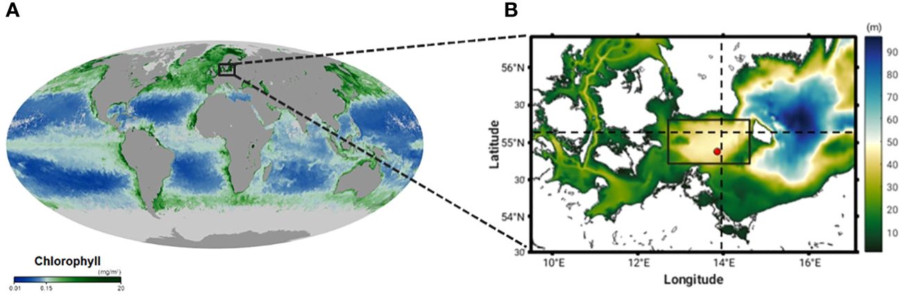
Figure 1 (A) Global distribution of chlorophyll-a, as seen by MODIS, May 2018 (source: https://earthobservatory.nasa.gov/global-maps/MY1DMM_CHLORA). Black rectangle indicates location of our study region. (B) Western Baltic Sea model domain bathymetry (m). Black rectangle shows the location of the Arkona Sea, the red dot indicates the location of Marnet Arkona Buoy long term mooring site (13°52’ E; 54°53’ N) and the dashed lines show the location of the transects used in the analysis.

Figure 2

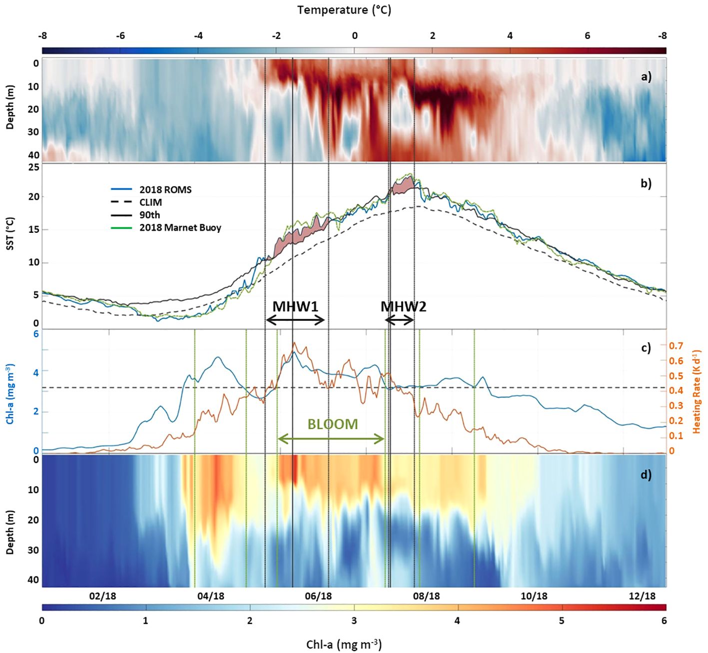
Figure 2 (A) modelled 2018 temperature anomaly at Marnet Arkona Buoy location (see Figure 1), 2018 temperature minus 90^th percentile 40 year climatology (1979 – 2019); (B) surface temperature at Marnet Arkona Buoy location: modelled (2018 ROMS), observed (2018 Marnet Buoy) and 30 year mean climatology (CLIM) and 90^th percentile (90^th) [using the NOAA OI SST V2 High Resolution Data Set (Huang et al., 2021)] (ROMS vs Marnet Buoy statistics: r²: 0.99, RMSE: 0.016, BIAS: -0.0010). Pink shaded areas indicate timing of MHW-1 and MHW-2, respectively; (C) modelled 2018 surface Chl-a (blue) and optically significant water constituent-induced surface heating rate (orange) at the Marnet Arkona Buoy location (dashed horizontal line indicates threshold value for onset of phytoplankton bloom (see text); (D) modelled 2018 water column Chl-a at the Marnet Arkona Buoy location. (grey dashed vertical lines indicate onset and end of MHW events, solid grey vertical line indicates day of detailed analysis during MHW event, green vertical dashed lines indicate start and end of phytoplankton blooms).

Figure 3

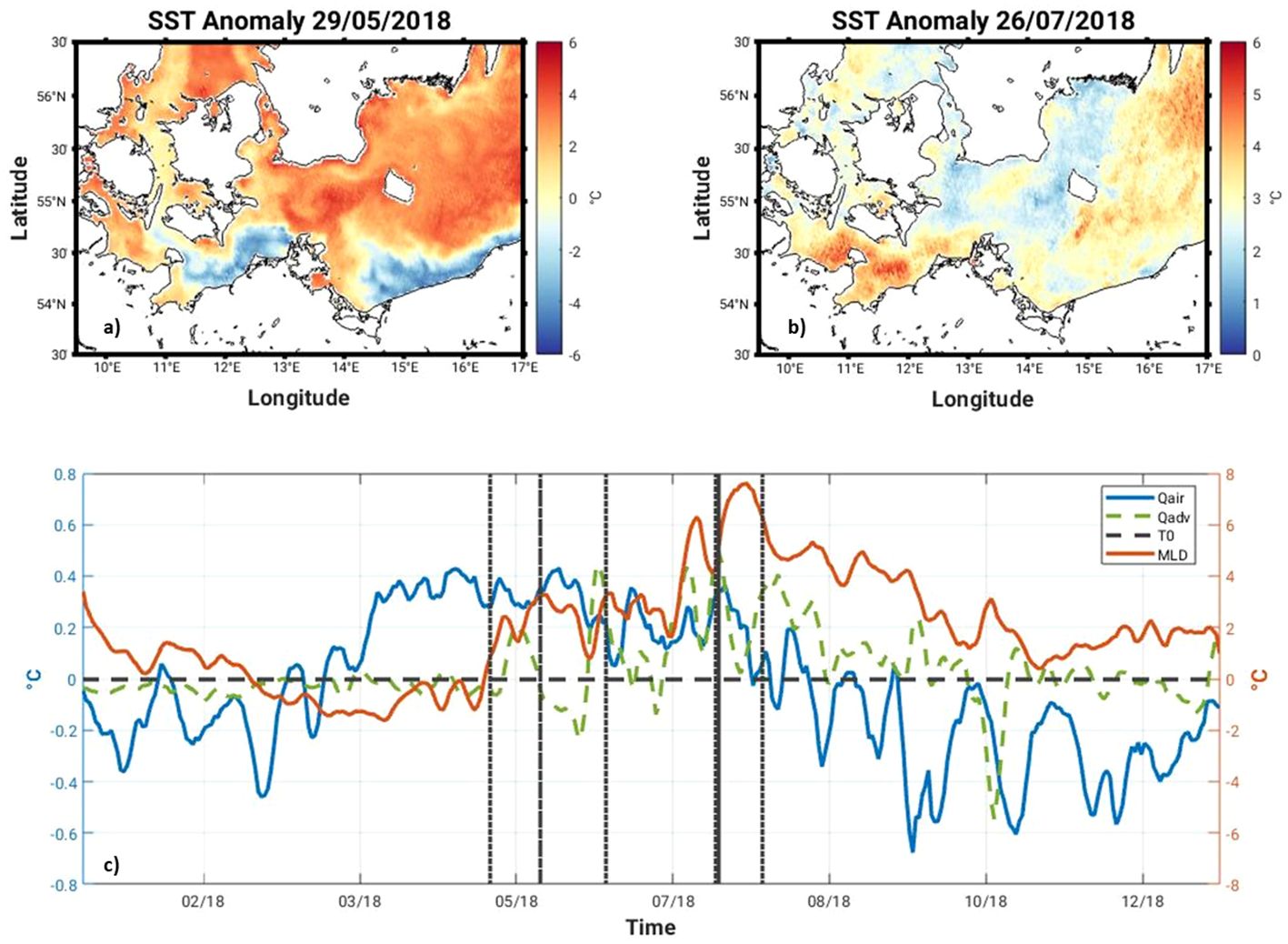
Figure 3 SST anomaly on 29 May 2018 (A) and 26 July 2018 (B) in the Western Baltic Sea; (C) cumulative contribution of the air-sea heat flux (blue line), horizontal advection (dashed green line) to the temperature anomaly and the mixed layer depth temperature anomaly (orange line) in the Arkona Sea in 2018. The SST Reanalysis (https://doi.org/10.48670/moi-00156) described in Høyer and She (2007) and Høyer and Karagali (2016) was used to calculate the SST anomalies shown in (A, B), while the Baltic Sea Physics Reanalysis (https://doi.org/10.48670/moi-00013) and the ERA-5 Global Reanalysis (https://doi.org/10.1002/qj.3803) described in Hersbach et al. (2020) were used to calculate the temperature anomalies shown in (C).

Figure 4

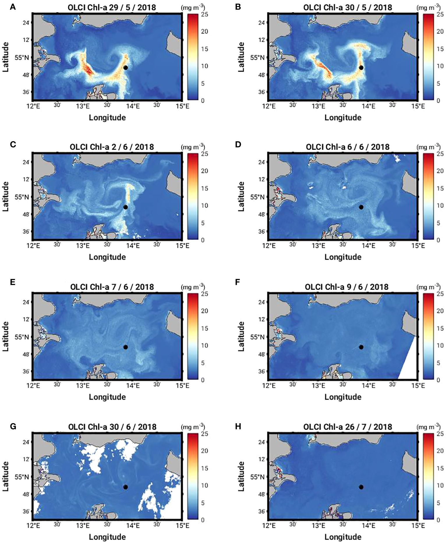
Figure 4 Sentinel-3 Ocean Land Cover Instrument (OLCI) L3 300 m resolution Chl-a on selected dates during the study period (A-H) 29, 30 May, 2, 6, 7, 9, 30 June, 26 July 2018, respectively). Black dot indicates the location of the Marnet Arkona Buoy long term mooring site.

Figure 5

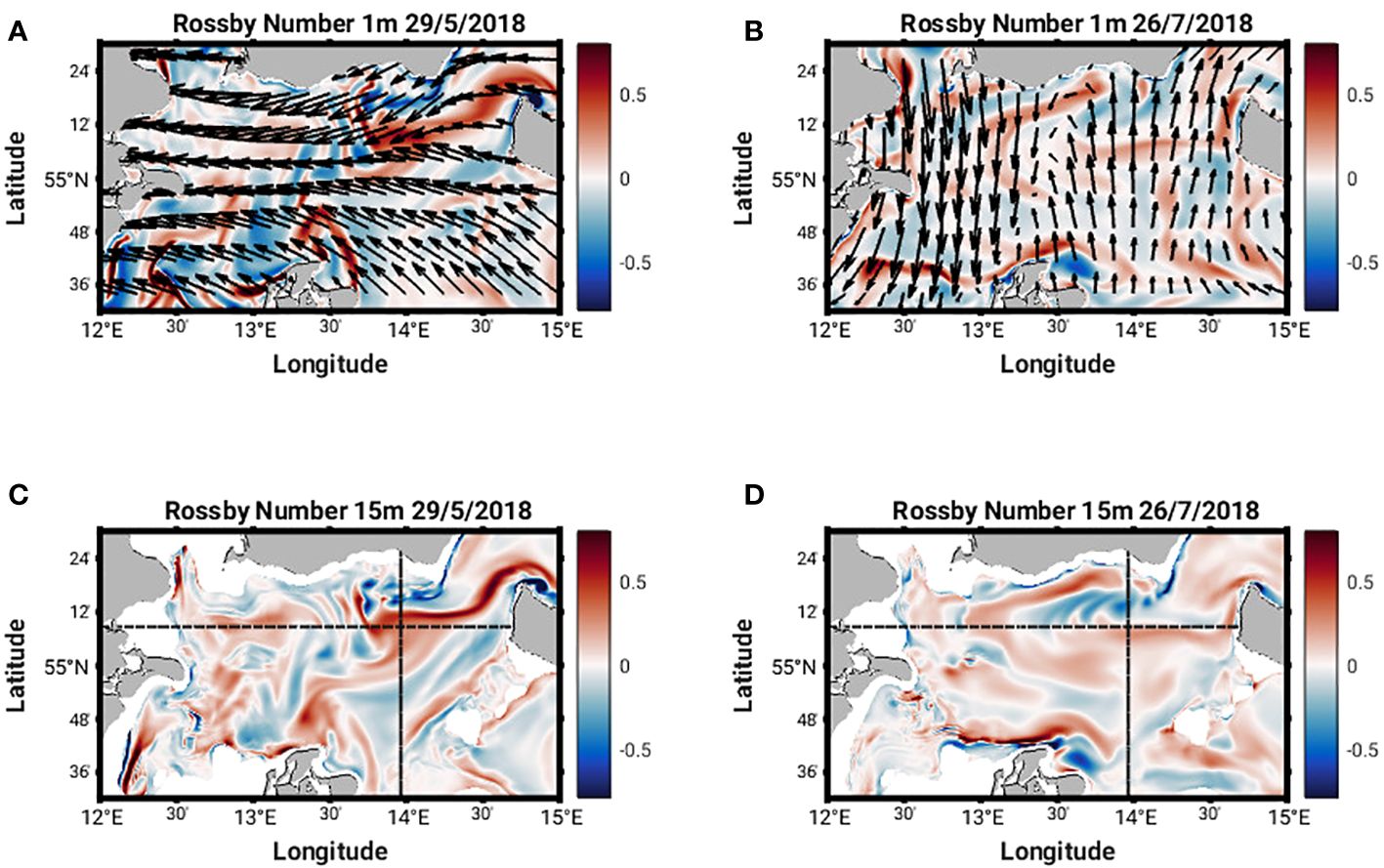
Figure 5 Rossby number at 1m and 15m on May 29 and July 26, 2018 (A–D). DWD-ICON 3-hourly surface wind vectors are overlaid on (A, B).

The Arkona Sea is an optically complex and biologically productive region, influenced by significant inputs of terrestrial organic matter from neighbouring rivers, especially colour dissolved organic matter (CDOM) during months of intensive mixing and high riverine discharge, March, April and November (Kowalczuk et al., 2006). In recent years, the growing season of phytoplankton in the Western Baltic Sea has extended from 159 days in the period 1988 to 1992 to 284 days in the period 2014 to 2017 (Wasmund et al., 2019a) in response to climate change. In 2018, Wasmund et al. (2019b) observed a shift in the spring bloom peak in the region to May with a prolonged period of moderate phytoplankton growth in the Arkona Sea primarily dominated by diatoms and dinoflagellates in May and June 2018.

2.2 Modelling the bio-optical ocean state in the Arkona Sea in 2018

We use the Regional Ocean Modelling System, ROMS, which drives the physics and the advection and diffusion of tracers, coupled with the Ecosim/Bio-Optic module (herein referred to as ROMS-BioOptic) which drives the ecosystem and a spectrally-resolved underwater light field. This setup is used to simulate the bio-optical ocean state in the western Baltic Sea for the year 2018 and is described in detail in Cahill et al. (2023) and references therein. Here we summarize important features. ROMS, is widely used for shelf circulation (e.g. Haidvogel et al., 2008; Wilkin et al., 2011) and coupled physical-biological applications (e.g. Fennel et al., 2006; Cahill et al., 2008; Fennel et al., 2008; Fennel and Wilkin, 2009; Cahill et al., 2016, Cahill et al., 2023). Ecosim is a carbon-based, ecological/optical modelling system (Bissett et al., 1999a, Bissett et al., 1999b) which was developed for simulations of carbon cycling and biological productivity. Ecosim simulates up to four phytoplankton functional groups each with a characteristic pigment suite which varies with the group carbon-to-chlorophyll-a ratio, C:Chl-a. Each groups’ C:Chl-a ratio varies between some maximum and minimum value, as a function of light or nutrient limitation. The properties of each functional group evolve over time as a function of light and nutrient conditions (i.e. NO₃, NH₄, PO₄, SiO and FeO). The maximum phytoplankton growth is modulated by temperature (Eppley, 1972). Loss processes are represented by grazing and excretion. Grazing accounts for the majority of the biomass sink in the model and is considered the closure term of the phytoplankton equations (Steele and Henderson, 1992). It is modelled as a Michaelis-Menten function based on the functional groups’ biomass (Bissett et al., 1999a). Marine and riverine sources of dissolved organic carbon (DOC and CDOC) are accounted for and explicitly resolved into labile (e.g. available for biological and photo-degradation) and relict (e.g. available for photo-degradation) forms. Dissolved inorganic carbon (DIC) is also accounted for. Riverine sources of carbon and nutrients are introduced via point sources. The underwater light field is spectrally-resolved at 5nm intervals between 400 and 700 nm. This allows for differential growth of different phytoplankton groups that have unique pigment complements.

Ecosim’s daylight module explicitly calculates the in-water spectrally-resolved absorption coefficients for phytoplankton, detritus and CDOM, the scattering and backscattering coefficients for phytoplankton and detritus, the average cosine, downwelling irradiance attenuation coefficient, K_d, in addition to the scalar, E₀, and downward, E_d, irradiance fields following Morel (1988). Cahill et al. (2023) recently updated the K_d formulation following Lee et al., 2005 which accounts for some of the optical complexity found in coastal waters. The spectrally-resolved underwater light field drives the evolution of all the water constituents in the ecosystem model (phytoplankton, detritus and CDOM), while the water constituents in turn determine the evolution of the light field in each layer by absorption and scattering of the light. This means that their contribution to the divergence of the heat flux (Morel, 1988) can be accounted for within the full hydrodynamic solution. Furthermore, water constituent-induced heating rates can be assessed (Cahill et al., 2023) and their impact on the ocean sea surface temperature can be communicated to the bulk flux formulation of the atmosphere in the modelling system.

The ROMS-BioOptic model was configured as described in Cahill et al., 2023 except with a higher resolution 600m horizontal grid in the Western Baltic Sea (see Table 1). A bulk flux atmosphere was forced with DWD-ICON output (Zängl et al., 2015) and river forcing including runoff and biogeochemistry (NO₃, NH₄, PO₄, SiO, DOC, CDOM and DIC) from 9 rivers which influence the region was derived from HELCOM PLC (Pollution Load Compilation) data (Neumann, pers. comm). Open boundaries to the north and east were forced with output from GETM physics using a combination of Chapman/Flather conditions for u and v velocities and transports, and Radiation + Nudging for temperature and salinity. This 3D setup is based on an existing GETM physics setup which has been previously evaluated and published (Gräwe et al., 2015a, Gräwe et al., 2015b). The Ecosim/Bio-Optic module was configured with four phytoplankton functional groups representative of small and large diatoms, large dinoflagellates and cyanobacteria. Initial conditions for the ecosystem model were obtained from previously evaluated and published output from the Ecological Regional Ocean Model (ERGOM) (Neumann et al., 2022). Our simulation period was 1 January to 31 December 2018. Daily averages and snapshots were output for the entire year. Hourly averages and snapshots were output for selected periods during both MHW events.

Table 1

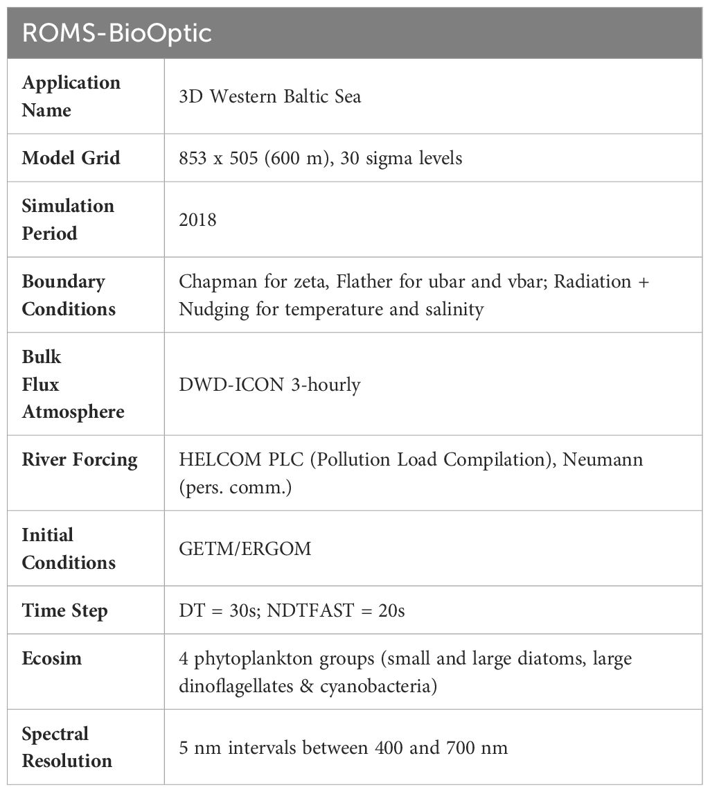
Table 1 Configuration of ROMS-BioOptic Western Baltic Sea Application.

2.3 Detecting MHW events

Following Hobday et al. (2018), surface temperature data from the BSH (Bundesamt für Seeschifffahrt und Hydrographie) MARNET Arkona Buoy, surface temperature output from our 600m ROMS-BioOptic simulation of the Western Baltic Sea and sea surface temperature data from the NOAA OI SST V2 High Resolution Dataset (Huang et al., 2021) were used to diagnose the May and July 2018 MHW events (Figure 2B; Table 2). The heat budget diagnostic approach summarized in Elzahaby et al. (2021) and based on Chen et al. (2015) and Bowen et al. (2017) was used to diagnose whether the MHWs were atmospheric-driven or oceanic-process driven (Figure 3C). Herein, the respective contributions of advection and air-sea heat flux anomalies to the mixed layer temperature tendency anomaly during each event are used to classify the drivers of MHW drivers. For this purpose, we used the Baltic Sea Physics Reanalysis (https://doi.org/10.48670/moi-00013) and the ERA-5 Global Reanalysis (https://doi.org/10.1002/qj.3803) described in Hersbach et al. (2020) to calculate the temperature anomalies.

Table 2

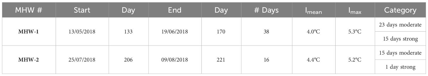
Table 2 Summary of MHW indices in the Arkona Sea in May and July 2018 (after Hobday et al., 2018).

2.4 Detecting phytoplankton blooms events

We define a bloom event following a threshold approach as used by Thomalla et al. (2011) and applied by Lorenz (2019) whereby the initiation of the bloom is understood to be the period of the year which registers a relative increase in chlorophyll concentration, irrelevant of the actual value. For our purposes, we define the threshold as the first day that surface Chl-a rises 15% above the annual median as follows:

CHL_S = CHL_MEDIAN + 0.15 * CHL_MEDIAN

Thus, the bloom start condition is:

CHL_t < CHL_S and CHL_t+1 > CHL_S

and, the bloom end condition is:

CHL_t > CHL_S and CHL_t+1 < CHL_S

In the run up to a bloom event, Chl-a tends to pulsate, often exceeding the threshold CHL_S for a short period of time (Racault et al., 2015). Therefore, events which are shorter than 7 days are not considered blooms and blooms which are less than 6 days apart are considered as one event.

2.5 Detecting and tracking eddy-like finite-time coherent structures

Building on the ideas applied by Vortmeyer-Kley et al. (2019), we use our modelled velocity output to search for three dimensional, eddy-like coherent structures in the Arkona Sea during the time of the MHW events. To do this, we apply a particle tracking method combined with the concept of finite-time coherent sets by Froyland and Junge (2018). In general, eddies can be described as separated waterbodies that minimally mix with or leak into their neighbourhood. This links the idea of eddies to the concept of finite-time coherent sets (Froyland and Junge, 2018; Froyland et al., 2019).

Froyland and Junge (2018) and Froyland et al. (2019) formulate the definition of a finite-time coherent set as the solution of the weak eigenproblem of the dynamic Laplacian Equation 1:

$\begin{array}{ll}-(\frac{1}{\left|\tau \right|}\sum _{t\in \tau }{D}^t)u=\lambda Mu& (1)\end{array}$

with u as set of eigenvectors, whose information correspond to the finite-time coherent set, λ as corresponding eigenvalues, D as the stiffness matrix and M as the mass matrix. The entries in the mass matrix M can be interpreted as the volume of all tetrahedrons built from a three dimensional triangulation from the tracer position in space at time t if the tracers are advected by a flow field for the time period τ. The entries in the stiffness matrix D correspond to the change of the shape of all tetrahedrons (details cf. Froyland and Junge, 2018). The information of the coherent sets in the eigenvectors is often not cleanly represented in the eigenvectors, so we use the SEBA algorithm (Froyland et al., 2019) to disentangle the information and save them into SEBA vectors whose entries represent the coherence level of the finite-time coherent sets.

The backbone of the above mentioned algorithm is a particle tracking that provides the trajectory calculations needed to describe the tracer positions in space in the time period τ properly. Here we use ROMSpath (Hunter et al., 2022; code at https://github.com/imcslatte/ROMSPath/tree/V1.0.0) and integrate massless tracer trajectories on a longitude-latitude-depth grid for 24h starting tracers from the same grid every hour in the period May 27, 2018 00:30am to June 2, 2018 01:30am and July 22, 2018 05:30am to July 29, 2018 11:30pm using the velocity fields from ROMS-BioOptic simulations.

We apply the approach by Froyland and Junge (2018) and Froyland et al. (2019) using their matlab scripts (https://github.com/gaioguy/FEMDL and https://github.com/gfroyland/SEBA) to calculate eddy-like finite-time coherent sets for each hour from the calculated tracer trajectories. We requested 40 eigenvectors and chose the first 25 SEBA vectors to find the largest and most coherent sets. From this assemblage of hourly detected eddy-like coherent sets, we build consecutive tracks of coherent sets by searching in the assemblage for sets of the same type (positive or negative 24h-mean relative vorticity in the centre of the set) that are spatially close to each other in successive time steps. (Spatially close to each other means that their inner product is larger than 0.75.) We define the 0.7 coherence level as the outer shapes of the eddy-like coherent sets in space. We take into account tracks of structures with a lifetime larger than 11 h, to consider only structures that live long enough to have an ecological impact.

3 Results

3.1 Characteristics of the May and July MHW events

Following the approach described in section 2.3, two MHW events were identified using observations from the Marnet Arkona Buoy in 2018 and the blended NOAA OI SST V2 product from Huang et al. (2021) (Figure 2B). Coincident modelled SST was compared to the Marnet Arkona Buoy data, to ensure the fitness for purpose of the physical model for the analysis of MHW surface and subsurface dynamics. The spatial extent of the MHWs on 29 May and 26 July 2018 was calculated as the SST anomaly using the SST Reanalysis (https://doi.org/10.48670/moi-00156) described in Høyer and She (2007) and Høyer and Karagali (2016) (Figures 3A, B). The MHW events are described in terms of their duration, mean intensity, I_mean, maximum intensity, I_max, and category (moderate, strong, severe or extreme) (Table 2). The May MHW (herein referred to as MHW-1) lasted 38 days, in which 23 are classified as moderate and 15 as strong. MHW-1 I_mean is 4.0°C and I_max is 5.3°C. The July MHW (herein referred to as MHW-2) lasted 17 days, in which 15 are classified as moderate and 2 as strong. MHW-2 I_mean is 4.4°C and I_max is 5.2°C. The heat budget diagnostic (Figure 3C) reveals that MHW-1 is an atmospheric-driven event, while MHW-2 is a mixed atmospheric- and horizontal advection-driven event.

There is very good agreement between our modelled ROMS-BioOptic sea surface temperature at Arkona Sea in 2018 and the observed sea surface temperature in 2018 (r^{2 =} 0.99, RMSE = 0.016, Bias = -0.001) (Figure 2B). The timing and surface characteristics of both MHW events are also captured very well in the model. This gives us confidence to examine the sub-surface properties of the 2018 modelled temperature anomaly using a 40 year modelled climatology (1979 – 2019) derived from General Estuarine Transport Model (GETM) simulations (Gräwe et al., 2015a) (Figure 2A).

The impact of MHW-1 extends to ca. 15 m during the first half of the event, after which it deepens over the full extent of the water column (Figure 2A). The maximum temperature anomaly (ca. 6°C) occurs a few days after the surface signature of MHW-1 has disappeared at depths between 15 and 25m. This maximum subsurface anomaly persists for about 3 days, after which it relaxes to ca. 4°C, but remains positive until the onset of MHW-2.

The subsurface impact of MHW-2 is much more pronounced compared to MHW-1. MHW-2 extends from the surface to ca. 15 m for the duration of the event with a temperature anomaly of ca. 4°C in the surface layer. Between 15 m and 30 m, a negative temperature anomaly (ca. 2°C) lies over a positive bottom temperature anomaly (ca. 3°C). The maximum temperature anomaly (ca. 8°C) is concentrated between 15 m and 20m for 15 days after the surface signature of MHW-2 has disappeared. Its extent then deepens from 15 m to about 30 m for further 10 days, following which it decays over a period of about 10 days, finally relaxing at the end of September.

3.2 Dynamics of phytoplankton blooms and MHWs

Following the threshold approach described in section 2.4, three distinct phytoplankton bloom periods were identified in the modelled Chl-a in 2018 (Figure 2C). The first bloom developed on 29^th March and persisted until 1^st May. Peak Chl-a concentration of 4.95 mg m^-3 occurred on 14^th April. A second bloom developed on 20^th May, 7 days after the onset of MHW-1. This persisted until 24^th July, one day before the onset of MHW-2. Peak Chl-a concentration of 5.4 mg m^-3 occurred on 29^th May and coincided with maximum water constituent-induced surface heating rates (Figure 2C). Modelled phytoplankton, CDOM and detrital absorption at 442 nm show that phytoplankton absorption dominates the diffuse attenuation coefficient at 492 nm during the second bloom event (Figures 6C–F) and thus contributes most to the surface heating rates. A third bloom event developed on 12^th August, two days after the end of MHW-2 event and persisted until 14^th September. Peak Chl-a concentration of 3.7 mg m^-3 occurred on 4^th September. We focus our attention on the evolution and decay of the 2^nd phytoplankton bloom event which is bookended by the MHW-1 and MHW-2.

Figure 6

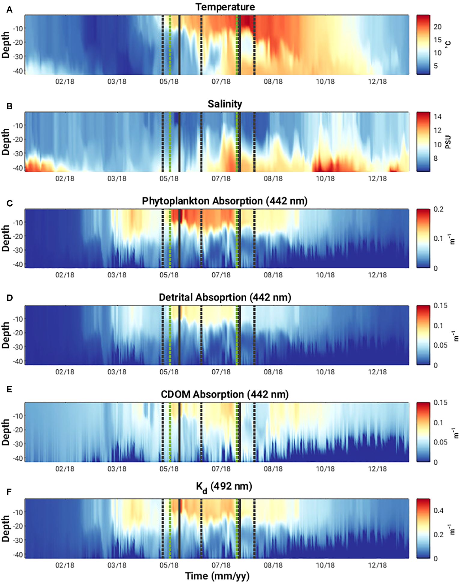
Figure 6 (A) Temperature, (B) salinity, (C-E) phytoplankton, detrital and CDOM absorption at 442 nm, respectively, and (F) the diffuse attenuation coefficient at 492 nm [K_d(492)] in Arkona Sea 2018. (Grey dashed vertical lines indicate onset and end of two MHW events, solid grey vertical line indicates day of detailed analysis during MHW event, green vertical dashed lines indicate start and end of the prolonged phytoplankton bloom event discussed in the text.).

Our analysis is centered on two separate days within the MHW-1 and MHW-2 events, 29 May and 26 July 2018. These days were selected for a number of reasons: they exhibit different bio-optical and biogeochemical responses to the MHW events; 29 May 2018 coincides with the maximum surface Chl-a concentrations and peak water constituent-induced heating rates during MHW-1 (Figure 2C); 26 July 2018 coincides with the end of the 2^nd phytoplankton bloom event, a steady decline in the water constituent-induced surface heating rates and the onset of MHW-2. A sequence of selected cloud-free Chl-a OLCI satellite data (Figure 4) starting from 29 May 2018 show a surface Chl-a signature persisting within the eddy-like structure for at least 10 days. As will be shown below, a similar eddy pattern was found in the model results in the same location at the end of May, although we do not expect the positions of the observed and simulated eddies to agree completely, because trajectories of eddies typically contain a stochastic element.

We evaluated the simulated surface Chl-a with coincident OLCI data. Ocean colour instruments receive most of their in-water signal from the surface down to one optical depth. When we refer to the simulated surface chlorophyll, we actually refer to the mean of the simulated chlorophyll over the first optical depth, rendering such satellite-derived and simulated chlorophyll concentrations comparable. In our area of interest, the OLCI data characterize the diffuse attenuation coefficient at 490 nm, K_d(490), to be about 0.5 m^-1 on 29 May 2018 and 0.25 m^-1 on 26 July 2018, resulting in a remotely sensed layer at 490 nm of about 2 m and 4 m, respectively. The evaluation shows that the model captures the surface dynamics of the phytoplankton bloom but highlights the difficulty in capturing the magnitude of the surface bloom event that is seen in the satellite data in May in the model (Supplementary Figures 1A-D). However, we would not expect the model to necessarily reproduce the magnitude of the bloom event observed by OLCI in May as these type of events are very difficult to reproduce in a model without data assimilation. Good agreement is seen between the model and OLCI data in July. Previous evaluations of modelled Chl-a and other water constituents using OLCI data also found good agreement between the model and OLCI data background values in the region (Cahill et al., 2023). The structure of the simulated surface Chl-a concentrations captures the extent of the eddy feature observed by OLCI in May (Supplementary Figure 1A). This supports our application of the model to explore the relationship between co-occurring MHWs and phytoplankton bloom events.

In order to explore the physical differences between the two MHWs further, we examine horizontal cross sections across the area of interest at 1 m and 15 m, and vertical transects across 13°58’ E and 55°8’ N. We use the Rossby number, Ro (defined as balance between the vertical component of the relative vorticity and planetary vorticity) to situate the flow regime (Figures 5, 7). This will be << 1 in mesoscale regimes, where planetary rotation constrains the flow and vertical stratification dominates, and O(1) in submesoscale flow regimes, where relative vorticity becomes important. Vertical sections of the horizontal (u and v) and vertical (w) velocity components (Figure 8) provide more information on the structure of the flow.

Figure 7

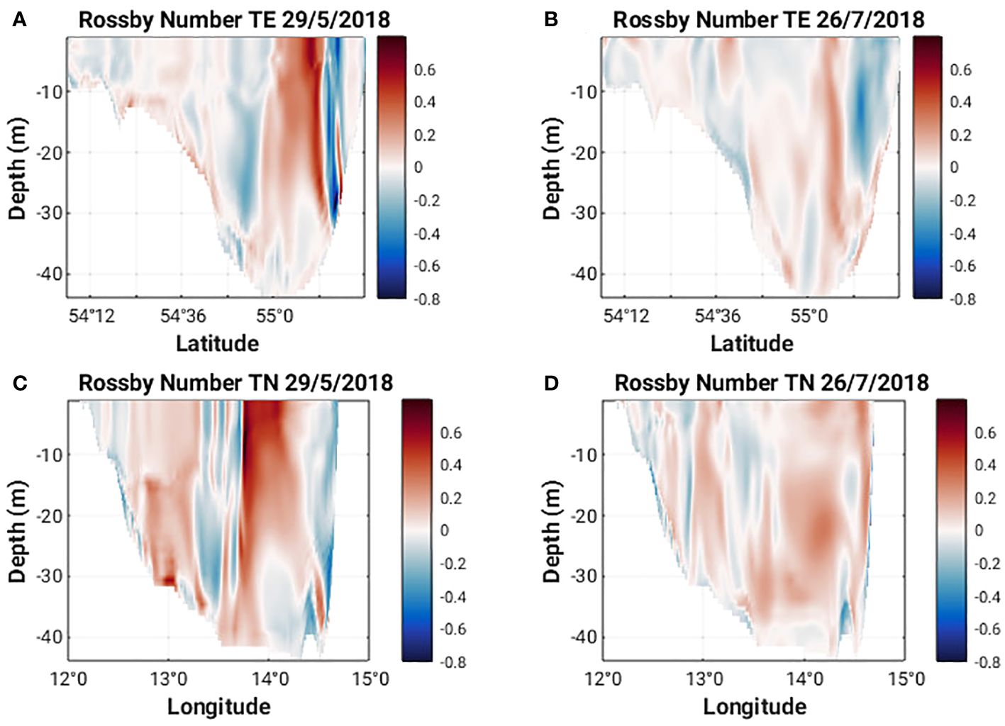
Figure 7 Rossby number along 13°58’ E (TE) and 55°8’ N (TN) on May 29 and July 26, 2018 (A–D).

Figure 8

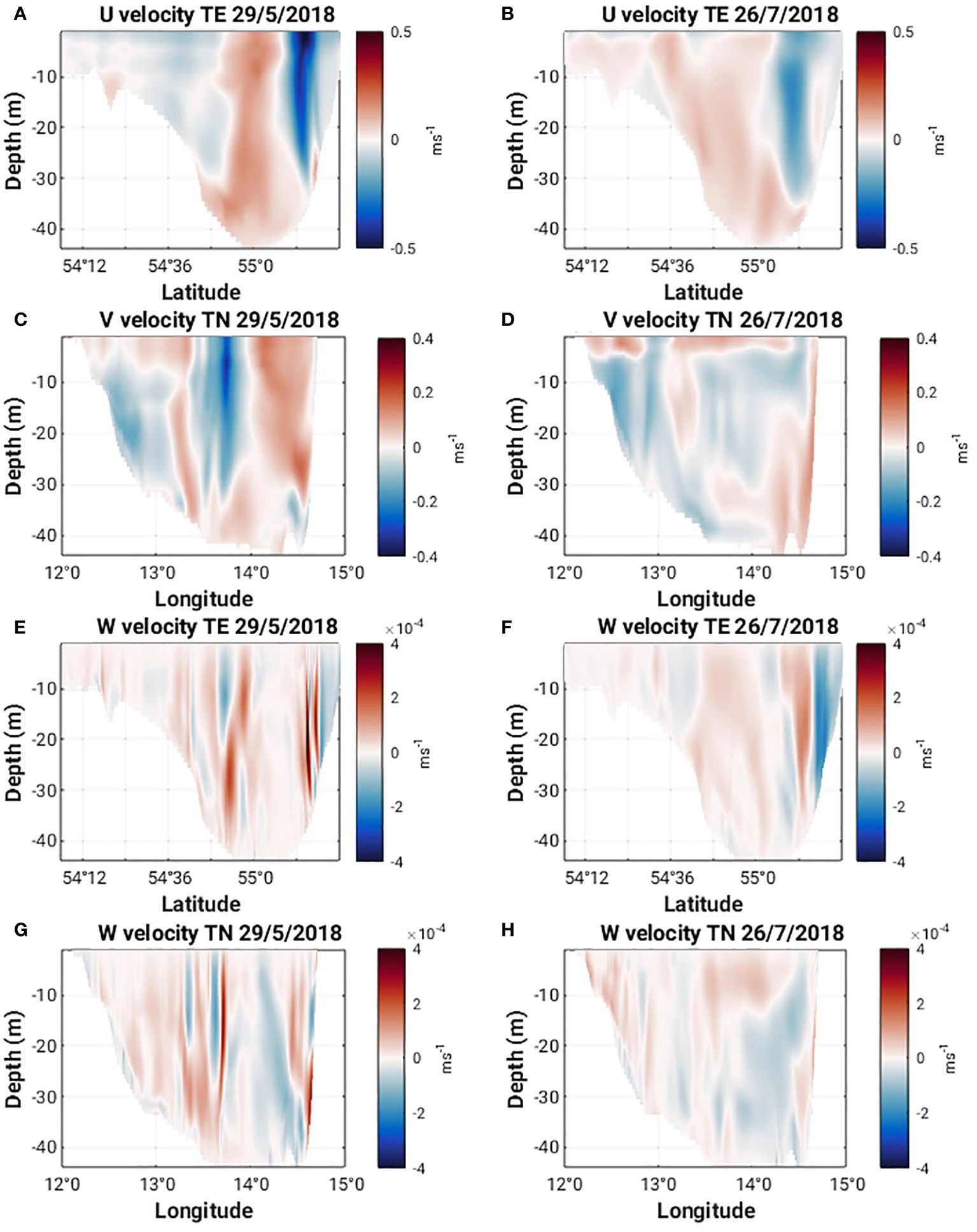
Figure 8 U, V, W velocities along 13°58’ E (TE) and 55°8’ N (TN) on May 29 and July 26, 2018.

3.2.1 29^th May 2018 (MHW-1)

Horizontal cross sections of Ro at 1 m and 15 m (Figures 5A, C) show a cyclonic eddy structure centered around 13°58’ E and 55°8’ N present on 29 May 2018. This structure extends from the surface to approximately 27 m depth (Figures 7A, C). The cyclonic nature of the structure is clear in the horizontal velocity components (Figures 8A, C) and relatively strong vertical velocities on the order of 10^-4 ms^-1 are seen on the northern and western flanks of the structure (Figures 8E, G) where Ro is +/- 0.8 (Figures 7A, C). The strong vertical velocities coincide with sharp lateral density gradients, a doming of isopycnals and upwelling of cooler subsurface water (Figures 9A, C). Converging north-southeasterly winds prevailed during this time (Figure 5A).

Figure 9

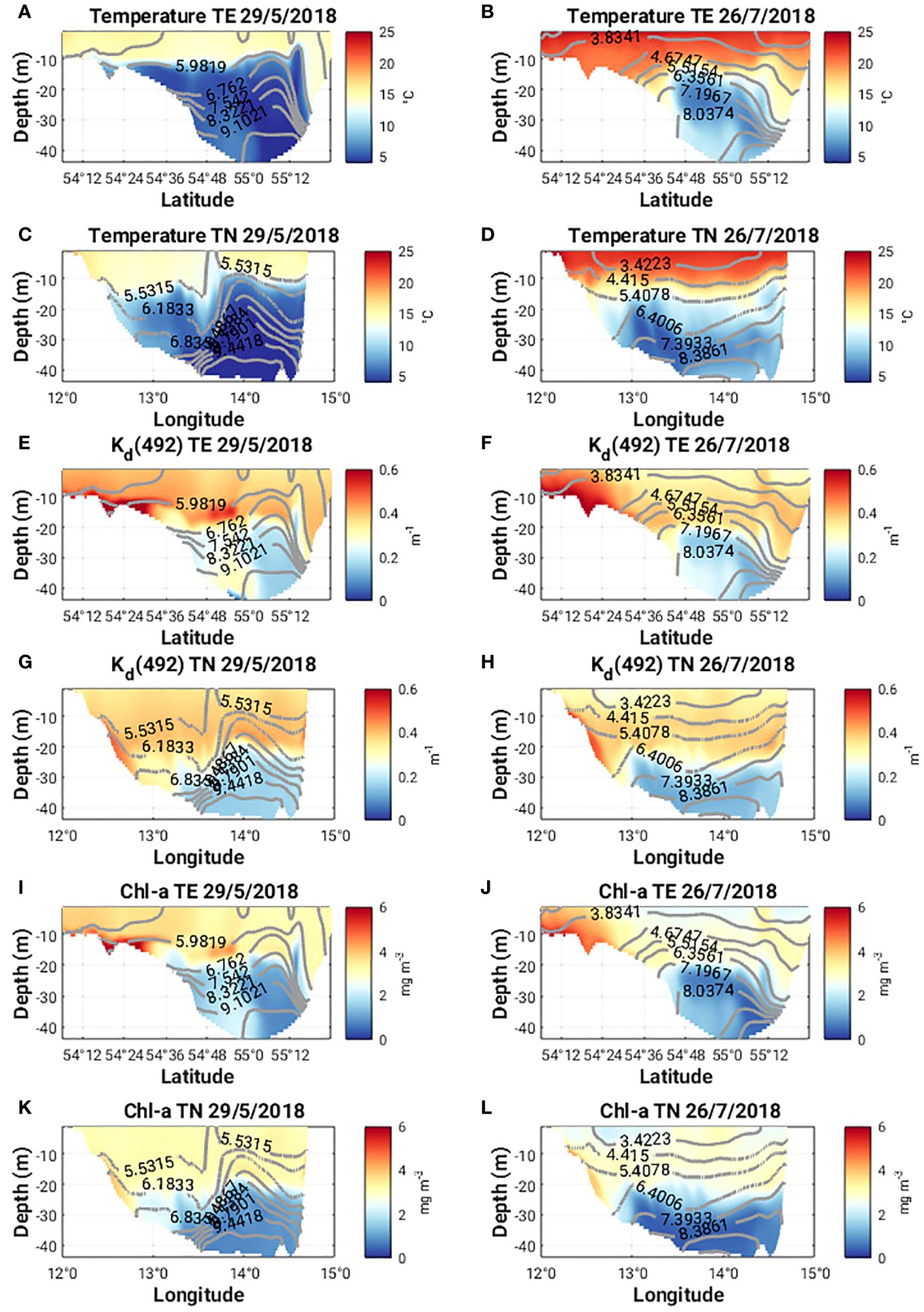
Figure 9 (A-D) Temperature (°C), (E-H) K_d(492) and (I-L) Chl-a along 13°58’ E (TE) and 55°8’ N (TN) on May 29 and July 26, 2018. Density contours are plotted as grey lines.

Horizontal cross sections of the diffuse attenuation coefficient at 492 nm, K_d(492) and Chl-a concentration at 1 m and 15 m on 29 May 2018, show higher subsurface values for both quantities compared to the surface values (Figures 10A, C, E, G). A subsurface Chl-a maximum accumulates on the southern flank of the eddy (Figure 9I). Sharp lateral gradients in both quantities also coincide with the sharp lateral density gradients (Figures 9E, G, I, K) and there are strong upward and downward vertical fluxes of Chl-a (ca. 60 mg m^-2 d^-1) along the northern, southern and western flanks of the eddy (Figures 11A, C).

Figure 10

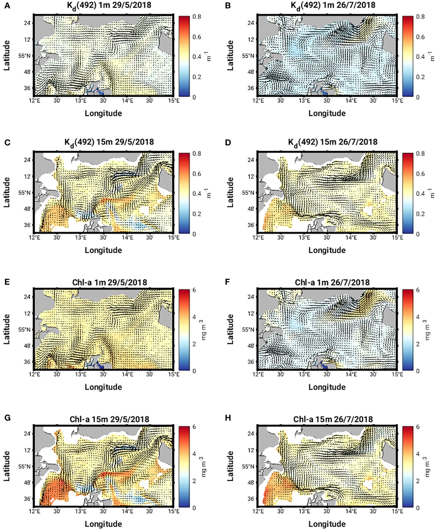
Figure 10 (A-D) K_d(492) and (E-H) Chl-a at 1m and 15m on May 29 and July 26, 2018.

Figure 11

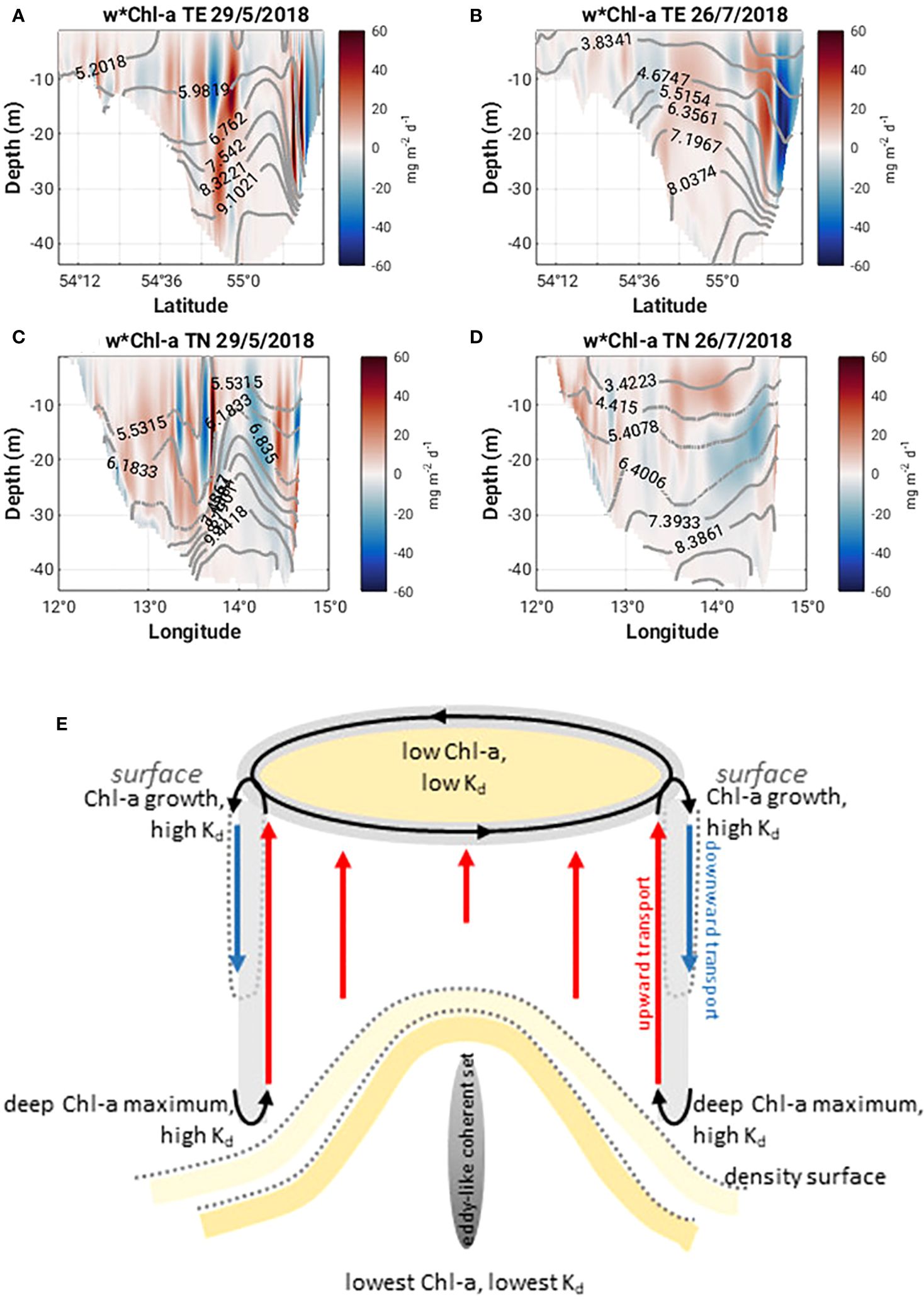
Figure 11 Vertical flux of Chl-a (w*Chl-a, mg m^-2 d^-1) along 13°58’ E (TE) and 55°8’ N (TN) on May 29 and July 26, 2018 (A-D). Density contours are plotted as grey lines; (E) simplified schematic of coupled surface-deep layer dynamics driven by cyclonic eddy at the peak of MHW-1.

3.2.2 26^th July 2018 (MHW-2)

The characteristics of Ro at 1 m and 15 m (Figures 5B, D, 7B, D) on 26^th July 2018 are quite different from those seen in May. The values are much smaller (ca. +/- 0.2) and no clear eddy-like structures are evident in the domain. Weaker northerly winds prevail east of 13°58’ E while southerly winds prevail west of 13°58’ E (Figure 5B). Along the southern Swedish coast, east of 13°30’ E, surface velocities are directed onshore (Figure 8D) and an overturning circulation is evident characterized by downwelling near the coast and upwelling offshore at 55°8’ N (Figure 8F). Some doming of isopycnals and upwelling of cooler subsurface water (Figure 9B) can also be seen at 55°12’ N. This coincides with a lateral gradient in the diffuse attenuation coefficient at 492nm, K_d(492) (Figure 9F) and Chl-a concentrations (Figure 9J) at this location. Strong downward and upward vertical fluxes of Chl-a (ca. 50 mg m^-2 d^-1) are also seen near the coast and offshore at 55°12’ N, respectively (Figure 11B). Horizontal cross sections of Kd(492) and Chl-a concentration at 1 m and 15 m on 26 July 2018, also reveal higher subsurface values for both quantities compared to surface values (Figures 10B, D, F, H). However, lateral gradients in temperature, Kd(492) and Chl-a values are absent along the 55° 8' N transect (Figures 9D, H, L) and vertical fluxes of Chl-a are weak (Figure 11D).

3.3 Coherent structures found during the MHW events

During MHW-1, a long-living, eddy-like coherent structure according to the methodology described in Section 2.5 is detected below the surface eddy structure visible in the satellite and modelled Chl-a and K_d(490/492) fields (shown in Figures 4A, 10C, G). The structure emerges on May 28, 2018 at 04:30am at 13°55’ E and 55°6’ N and dies out on June 02, 2018 at 01:30am at 13°47’ E and 55°0.6’ N, travelling about 13 km (Supplementary Figure 2). The structure extends during its life time from about 24 m to about 44 m depth and has a mean volume of 0.4 km³ (an equivalent diameter of about 4 km if the structure is assumed to be cylindrical). During its lifetime, the tracers inside the structure show tendencies of upward motion (Figures 12A, B) which coincides with a doming of isopycnals above the structure (Figures 9A, C). Tracers seeded along a rectangular slice at 13°58’ E and 55°8’ N in May 29, 2018 at 11:30am show a strong semi-circular shaped south-eastward displacement after 24h of integration (Figures 12A, B) in the surface layer which correlates with an increase in Chl-a at the eddy boundaries (Supplementary Figure 2). During MHW-2, the tracer displacement starting from the same slice on July 26, 2018 at 11:30am shows a less dynamic displacement into different directions with a small trend towards the north in the surface layers (Figures 12C, D), consistent with the onshore displacement of surface waters and overturning circulation seen earlier in the vertical velocity fields (Figure 8F), and the vertical fluxes of Chl-a (Figure 12B).

Figure 12

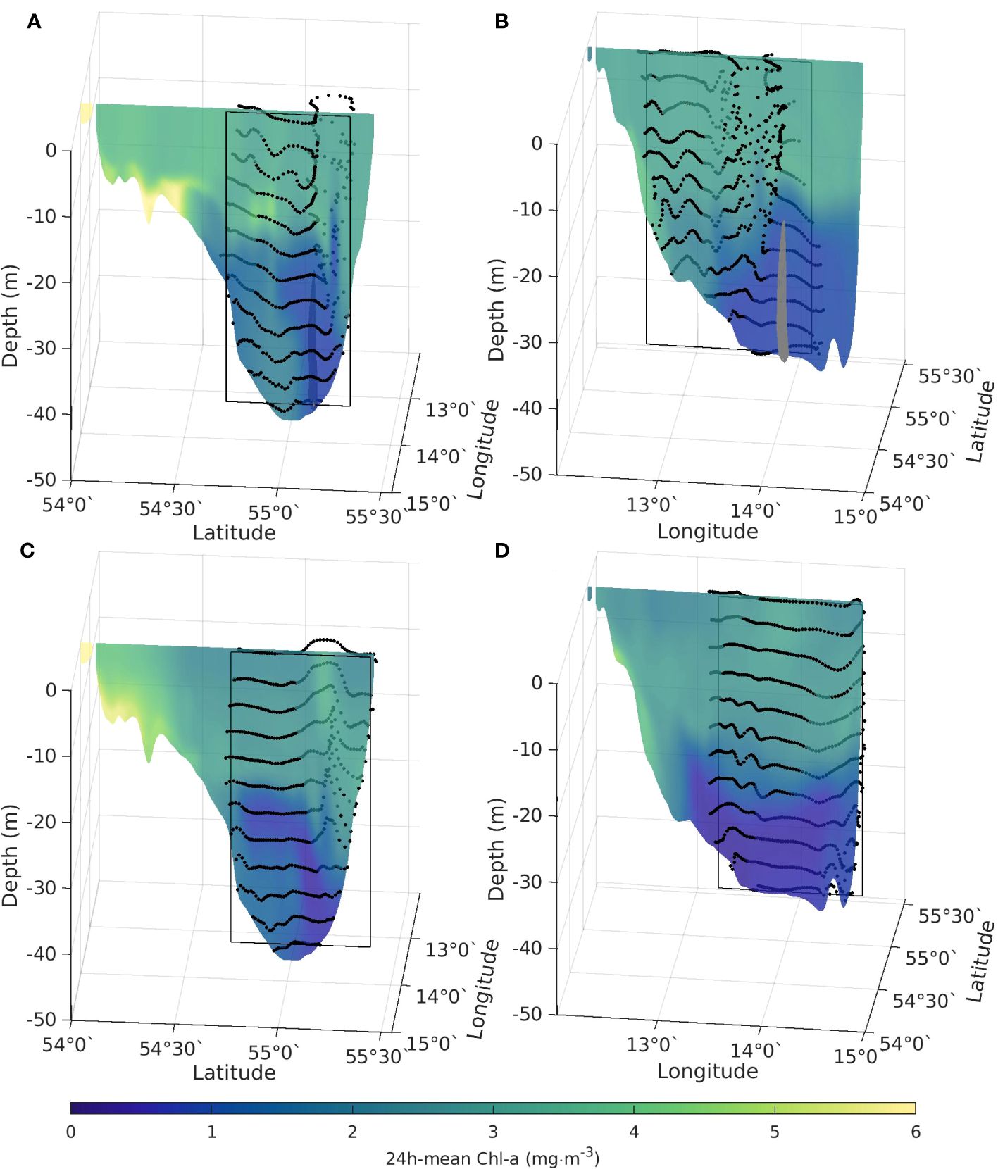
Figure 12 (A) 24h-mean chlorophyll along a 13°58’ E slice (B) 55°8’ N slice) and the tracer position (black dots) after 24h of particle tracking starting on a grid in the black rectangle at May 29, 2018 11:30am. The gray structure corresponds to the position of the coherent structure at that time. (C) 24h-mean chlorophyll along a 13°58’ E slice (D) 55°8’ N slice) and the tracer position (black dots) after 24h of particle tracking starting on a grid in the black rectangle at July 26, 2018 11:30am.

Comparing the spatial dynamics of the May coherent structure with the Chl-a content in the water column for May 28 to May 31 (Supplementary Figure 2), we found that the structure correlates with a low Chl-a patch during the whole period of time and weak vertical fluxes of Chl-a. The long lifetime of the deeper coherent structure in May 2018 appears to be linked to the persistence of the eddy in the top 30m and the dynamics of the deeper layers are more coupled to the surface layers during MHW-1. In July, a stronger thermocline de-couples the dynamics between the surface and deeper layers. Combined with onshore winds in July, the tendency is rather to support onshore displacement of surface waters toward the Swedish coast, and a coastal overturning circulation cell.

The high Chl-a patch that bends around the southwestern edge of the eddy in May (Figure 10G) can be interpreted as the impact of a “sticking” (unstable) manifold (Lehahn et al., 2007) on the distribution of particles in the flow. Stable and unstable manifolds act as organizing structures of the flow separating regions of different dynamical behaviour (Prants, 2013). Due to the attracting properties of the unstable manifold, nutrients and plankton are collected along it. This “sticking” manifold is visible as a dark blue singular line in Figure 13A which also correspond to the high K_d and Chl-a patch seen in Figures 10C, G. The manifold extends down into the upper water column, as seen in Figure 13B and provides a three-dimensional transport barrier around the southern, southeastern and eastern edge of the eddy. This mechanism could also explain the surface Chl-a patterns seen in May in the OLCI data (Figure 4).

Figure 13

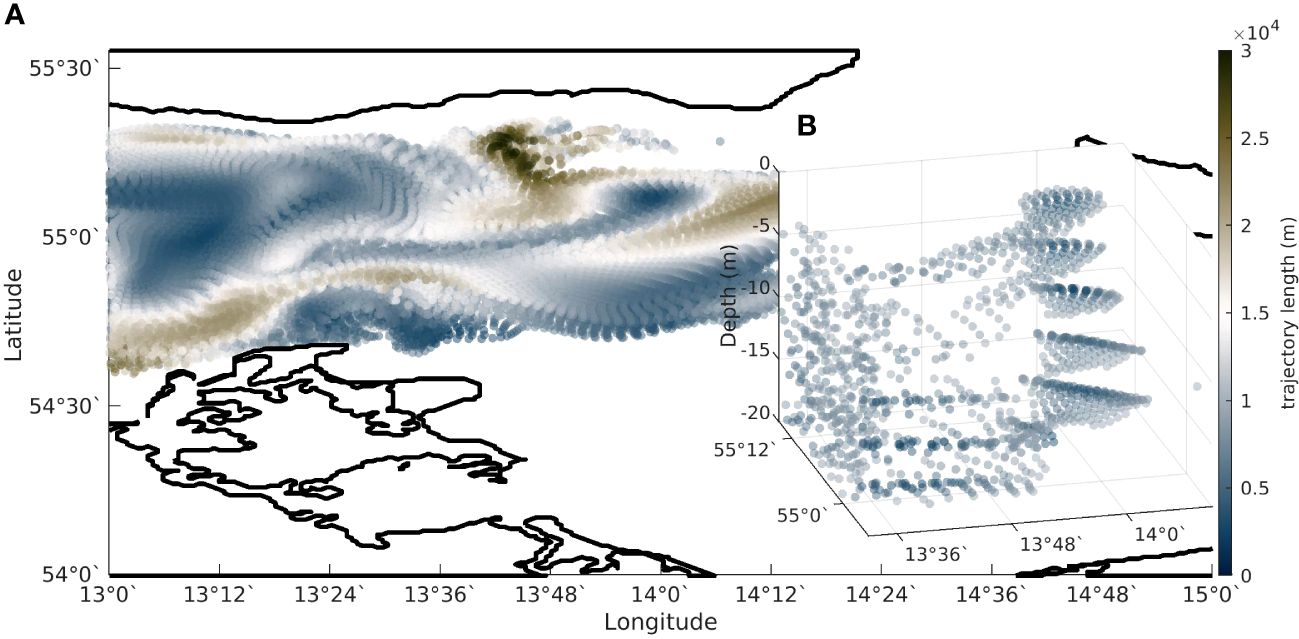
Figure 13 Sticking manifold calculated as the trajectory length of backward integrated trajectories of the velocity field (Prants et al., 2011; Prants, 2013; Jimenez Madrid and Mancho, 2009; Mendoza and Mancho, 2010). The values of the trajectory length are assigned to the starting points of the trajectories. All these values make up a three-dimensional map. (A) Map of trajectory length of for 24h backward integrated trajectories starting at May 29, 2018 11:30am. The sticking manifold is displayed as the dark blue singular line. (B) Three-dimensional view of the sticking manifold.

4 Discussion

We examined two different MHW events in 2018 which bookmark the evolution and decay of a phytoplankton bloom in the Arkona Sea. Our objective was to explore the relationship between co-occurring MHW and phytoplankton bloom events with the following specific questions in mind:

1. How, and under which circumstances, do MHWs contribute to the initiation of phytoplankton blooms?

2. Which dynamics play a role in sustaining the bloom?

3. How deep and for how long is the impact of the MHW felt?

4. What role, if any, do MHWs play in terminating a phytoplankton bloom?

5. Do phytoplankton blooms have an enhancing effect on MHWs by creating a positive feedback from water constituent–induced surface heating?

Marine heatwaves are typically associated with shallower mixed layer depths (Hayashida et al., 2020). Cook et al. (2022) show that atmospheric pressure systems, wind speed and latent heat fluxes are important contributing factors to the generation and decline of MHWs. Surface flux-driven MHWs are shallower and occur predominantly in summer (Elzahaby et al., 2021). MHW-1 develops mid-May in parallel with a strengthening and shoaling of the seasonal thermocline (Figure 6A). The heat budget diagnostic confirms that MHW-1 is an atmospheric-driven event. Surface salinity also decreases during the onset of MHW-1 (Figure 6B), consistent with Elzahaby and Schaeffer (2019) whereby increased anomalous solar radiation and decreased wind stress act on the latent heat flux to reduce evaporation. Given sufficient light and supply of nutrients, phytoplankton growth will occur. Increased phytoplankton biomass in the surface will increase the surface temperature due to absorption of light by phytoplankton in the surface layer. A thermal structure is established in the water column which will impact the growth, transport and fate of phytoplankton biomass. The availability of light below the productive layer will be strongly reduced. In the absence of other physical transport processes on timescales which are relevant for phytoplankton growth (Kuhn et al., 2019), nutrients will become depleted in the surface layer, the supply of nutrients from deeper waters will be inhibited by the stronger thermocline mid-summer, and phytoplankton growth will be expected to decrease.

A model study by Hayashida et al. (2020) shows that background nutrient conditions will determine the response of phytoplankton blooms co-occurring with MHWs. Generally, they find that in nutrient poor waters, blooms are weaker during MHWs, whereas in nutrient-rich waters, blooms are stronger during MHWs. However, transport dynamics play a critical role in the supply of nutrients to the surface mixed layer. In our scenario, wind driven surface circulation underpins the development of a series of cyclonic eddies in May and June over the Arkona Basin. The eddy we focus on late May has Ro O(1), an indication that relative vorticity is the same order of magnitude as the Coriolis force, that circulation has departed from geostrophy, and that ephemeral submesoscale dynamics may be at play. Indeed, large vertical velocities (ca. 35 m d^-1) along the edges of the eddy are seen, giving rise to upwelling and downwelling along the boundaries of the eddy (Figure 8E, G; Supplementary Figure 2). Vertical fluxes of Chl-a are between 40 and 60 mg m^-2 d^-1, along the north- and south-western boundaries of the eddy (Figures 11A, C). Upwelling vertical fluxes may also transport nutrients to the surface contributing to sustained phytoplankton growth. This potential coupling of surface and subsurface dynamics is illustrated schematically in Figure 11E.

A number of mechanisms relate the role of submesocales and mesoscale eddies and their impact on the horizontal and vertical distribution of Chl-a. Submesoscale phytoplankton patchiness is often visible in satellite images (Lapeyre and Klein, 2006; Levy et al., 2012), whereas in the Baltic Sea intense submesoscale activity has been observed through its imprint on cyanobacteria blooms (McWilliams, 2016). Several dynamical mechanisms that occur in the submesoscale regime, e.g., frontal subduction and submesoscale restratification (Chrysagi et al., 2021), have been proposed to explain not only the surface but also the subsurface biogeochemistry signals (Hosegood et al., 2013; Levy et al., 2018). Eddy stirring which describes the direction of rotational flow of the eddy field, is known to be a source of phytoplankton patchiness (Abraham, 1998; Martin, 2003) and will determine the position of the chlorophyll anomaly and the direction of propagation of the eddy relative to the ambient chlorophyll field (McGillicuddy, 2016). A cyclonic eddy in the northern hemisphere will result in a positive anomaly in the southwest quadrant, a negative anomaly in the northeast quadrant and westward propagation. We see a Chl-a maximum accumulate on the southern flank of the eddy at about 15 m depth (Figure 9I).

According to Mahadevan (2016), the vertical transport of nutrients into the euphotic zone can be achieved either by the vertical movement of the nutrient-rich isopycnal layers or by an advective flux. The former occurs mainly in the presence of internal waves or within mesoscale eddies but at different timescales. Eddies typically mix properties along isopycnals, and diapycnal mixing is considered to be weak. On the other hand, the advective flux of nutrients dominates in submesoscale features and tends to occur along the vertically tilted isopycnals. Reißmann et al., 2009, show that in the Baltic Sea, mesoscale eddies, known as Beddies may contribute to vertical mixing through different mechanisms. In particular, Beddies can contribute to the diapycnal mixing, inside the permanent halocline region, either through the vertical displacement of water and isopycnals, or through their decay. Another potential yet indirect mechanism through which Beddies may impact the halocline mixing, is through their interaction with internal waves, although this remains to be verified. Nevertheless, the exact dynamical mechanisms by which eddies might affect vertical mixing, are out of the scope of this study, since here we focus mainly on the co-occurence of MHWs and phytoplankton blooms.

We see indications of an unstable “sticking” manifold (Figure 13A), arising from geostrophic eddy stirring, acting as both a horizontal transport barrier for Chl-a and a facilitator of phytoplankton growth mediated by nutrient upwelling, as observed by Lehahn et al. (2007). The manifold extends down into the upper water column (Figure 13B) and provides a three-dimensional transport barrier around the southern, southeastern and eastern edge of the eddy. The emergence of the long-living, eddy-like coherent structure below the surface eddy structure illustrates the role of the surface eddy in isolating a cold, dense, sub-surface, low Chl-a water body below the surface eddy pointing at a coupling of surface and subsurface dynamics (Figures 12A, B; Supplementary Figure 1). Outcropping of isopycnals and upwelling of colder water along the southwestern edge of the eddy (as seen in Figures 9A, C) produce cold sea surface temperature anomalies which would tend to draw heat into the ocean from the atmosphere, further increasing stratification in those features relative to ambient waters. The complexity of eddy-induced transport mechanisms and biophysical interactions is reviewed in depth in McGillicuddy (2016) and references therein).

According to Levy et al. (2018), the combination of the seasonal distribution of light and the vertical supply of nutrients through ephemeral fronts are essential ingredients for sustained phytoplankton growth. The timing of the onset of MHW-1 in May provides optimal light conditions which, given sufficient supply of nutrients, may contribute to the initiation of the phytoplankton bloom. The series of eddies which ensue, support both geostrophic eddy stirring and transient submesoscale dynamics along the edges of the eddies which may in turn provide both an upward and downward transport path for nutrient fluxes and carbon export (Callbeck et al., 2017; Ruiz et al., 2019).

It is important to note that the surface signature of both MHWs, does not represent the deeper signature and impact of the MHWs. Schaeffer and Roughan (2017) suggest that vertical mixing, in combination with downwelling favourable winds, can weaken stratification and enable MHWs to extend deeper than the surface mixed layer, thus homogenizing the water column. We see a deepening of the thermocline take place in MHW-1 (Figure 6A) shortly after the peak in Chl-a concentration and associated water constituent-induced heating rate at the end of May (Figure 4).

Water constituent-induced surface heating increases with the onset the bloom, and peaks in the middle of MHW-1 at 0.7 K d^-1 (Figure 4). This increase in water constituent-induced surface heating is clearly a response to increases in Chl-a concentration and is directly related to the absorption of light by phytoplankton (Figure 6C) and to a lesser extent, detrital and CDOM absorption (Figures 6D, E). MHW-1 contributes to the initiation of the bloom, which in turn contributes to an increase in water constituent-induced heating rates. A recent study by Cahill et al. (2023) found that, in 2018, water constituent-induced surface heating rates in the Western Baltic Sea could reach up to 0.4 to 0.8 K d⁻¹ during the period April to September. Moreover, this water constituent-induced surface warming resulted in a mean loss of heat (ca. 5 W m⁻²) from the sea to the atmosphere, primarily in the form of latent and sensible heat fluxes. Thus, the phytoplankton bloom may have an enhancing effect on the MHW as a consequence of its contribution to surface warming but air-sea energy flux exchange plays a role in regulating this.

MHW-2 develops late-July, and coincides with a re-stratification of the water column, a stronger, shallower thermocline and the end of the phytoplankton bloom. The Rossby number is small, indicating that there is no significant submesoscale activity. The end of the phytoplankton bloom is preceded by a period where the temperature anomaly extended the full depth of the water column. Zhan et al (2023) examine the roles of atmospheric forcing-driven and oceanic processes-driven MHWs in driving changes in Chl-a concentrations and phytoplankton biomass. They show that atmospheric forcing-driven MHWs (like MHW-1) tend to increase Chl-a concentrations and phytoplankton biomass, while oceanic processes-driven MHWs tend to decrease Chl-a concentrations and phytoplankton biomass. The heat budget diagnostic shows MHW-2 to be a mixed atmospheric-and horizontal advection-driven event. Indeed, advection of higher salinity, warmer bottom water precedes MHW-2 (Figures 6A, B). Changes in the seasonality of saltwater inflows from the North Sea to the Baltic Sea has been shown to cause exceptional warming trends in the Western Baltic Sea (Barghorn et al., 2023). The stronger thermocline in MHW-2 de-couples the dynamics between the surface and deeper layers and any supply of nutrients to the surface from the deeper waters is cut off. Only along the Swedish coast do we see evidence of some downwelling and upwelling (Figure 8F) and strong vertical fluxes of Chl-a (ca. 40 mg m^-2 d^-1) (Figure 11B).

The persistence (up to 35 days between 15 m and 20 m) of the subsurface maximum temperature anomaly after the surface signature of MHW-2 has disappeared is remarkable. This underscores the importance of considering subsurface hydrography in order to fully understand the impact of MHWs on biological production (Schaeffer and Roughan, 2017). Moreover, the vertical extent of the subsurface temperature anomaly will play a role in the distribution of horizontal gradients in density and intensification of fronts, and thus determine transport pathways for nutrients and carbon.

In summary, we find that in the shallow Arkona Sea, the timing of atmospheric driven MHWs can contribute to the initiation of a phytoplankton bloom by providing the optimal conditions for phytoplankton growth. The vertical component of an eddy-like structure’s vorticity balance determines the strength of coupling between the surface and subsurface dynamics, and seems to provide a vertical transport pathway for nutrients. These coupled dynamics might in turn contribute to sustaining phytoplankton growth. Depth-integrated phytoplankton will be restricted within a shallower mixed layer which will in turn increase surface heating. Thus, phytoplankton blooms may have an enhancing effect on MHWs as a consequence of their contribution to surface warming but air-sea energy flux exchange will play a role in regulating this exchange. The subsurface signature of MHWs is often stronger and persists for longer than its surface signature. Moreover, the subsurface signature of the MHW plays a critical role in de-coupling surface and subsurface dynamics and terminating a phytoplankton bloom.

Remotely sensed ocean colour data provides a window into the spatial complexity of optically active constituents in surface waters and how these constituents are transported by surface circulation. Knowledge of coincident surface winds, can provide some clues as to what may be occurring subsurface but used in tandem with 3D biogeochemical ocean models, it is possible to see how surface and subsurface dynamics are really connected and extend our knowledge on surface layer processes obtained from satellite data. In the last decade, ocean colour observations have been recognized as essential climate variables (ECVs) and become an integral part of ocean observing systems. While the volume of this data set increases, it remains underexploited in operational biogeochemical modelling and forecasting. Moreover, the availability of new satellites, automated measurement systems such as Bio-Argo floats, drones, and computational resources presents both a challenge and an opportunity to advance integrated observing systems which combine optical observations, including remotely sensed ocean colour, with biogeochemical models to monitor and predict the impact of extreme events on biogeochemical cycles and ecosystem functioning.

Data availability statement

Publicly available datasets were analyzed in this study. This data can be found here: NOAA OI SST V2 High Resolution Dataset: https://psl.noaa.gov/data/gridded/data.noaa.oisst.v2.highres.html OLCI Level 3 300m Baltic Sea Ocean Colour Plankton, Transparency and Optics NRT daily observations, CMEMS: https://doi.org/10.48670/moi-00294. The ROMS-BioOptic model code can be accessed at https://www.myroms.org. The code of ROMSpath can be found at https://github.com/imcslatte/ROMSPath/tree/V1.0.0. For the calculation of the coherent sets the 3d version of the matlab scripts https://github.com/gaioguy/FEMDL and https://github.com/gfroyland/SEBA were used. Data of the tracer trajectories and the coherent set tracks upon request by RVK.

Author contributions

BC: Writing – review & editing, Writing – original draft, Visualization, Validation, Project administration, Methodology, Investigation, Funding acquisition, Formal analysis, Data curation, Conceptualization. EC: Writing – review & editing, Visualization, Investigation, Conceptualization. RV-K: Writing – review & editing, Visualization, Investigation, Formal analysis, Conceptualization. UG: Writing – review & editing, Resources.

Funding

The author(s) declare financial support was received for the research, authorship, and/or publication of this article. BC was supported by funding from the German Research Foundation (Grant No. CA 1347/2-1, 2018 to 2021, Temporary Position for Principal Investigator). EC was supported by funding from the CONMAR (CONcepts for conventional MArine Munition Remediation in the German North and Baltic Sea) project. RV-K would like to thank DFG Project VO 2508/1-1 for funding. UG was supported by the Federal Ministry of Education and Research (BMBF, funding code 03F0860H), within the project: ECAS-Baltic project: Strategies of ecosystem-friendly coastal protection and ecosystem-supporting coastal adaptation for the German Baltic Sea Coast. The authors gratefully acknowledge the computing time granted by the Resource Allocation Board and provided on the supercomputer Lise and Emmy at NHR@ZIB and NHR@Göttingen as part of the NHR (North German Supercomputing Alliance) infrastructure. The calculations for this research were conducted with computing resources under the project ID bek00027.

Acknowledgments

BC and RV-K would like to thank John Wilkin, Rutgers University for his advice on setting up the ROMSpath simulations.

Conflict of interest

The authors declare that the research was conducted in the absence of any commercial or financial relationships that could be construed as a potential conflict of interest.

Publisher’s note

All claims expressed in this article are solely those of the authors and do not necessarily represent those of their affiliated organizations, or those of the publisher, the editors and the reviewers. Any product that may be evaluated in this article, or claim that may be made by its manufacturer, is not guaranteed or endorsed by the publisher.

Supplementary material

The Supplementary Material for this article can be found online at: https://www.frontiersin.org/articles/10.3389/fmars.2024.1323271/full#supplementary-material

References

Abraham E. (1998). The generation of plankton patchiness by turbulent stirring. Nature 391, 577–580 doi: 10.1038/35361

CrossRef Full Text | Google Scholar

Barghorn L., Meier H. E. M., Radtke H. (2023). ). Changes in seasonality of saltwater inflows caused by exceptional warming trends in the Western Baltic Sea. Geophysical Res. Lett. 50, e2023GL103853doi: 10.1029/2023GL103853

CrossRef Full Text | Google Scholar

Belkin I. (2009). Rapid warming of large marine ecosystems. Prog. Oceanography 81, 207–213 doi: 10.1016/J.POCEAN.2009.04.011

CrossRef Full Text | Google Scholar

Benthuysen J. A., Oliver E. C. J., Feng M., Marshall A. G. (2018). Extreme marine warming across tropical Australia during austral summer 2015–2016. J. Geophys. Res. Oceans 123, 1301–1326 doi: 10.1002/2017JC013326

CrossRef Full Text | Google Scholar

Bissett W., Walsh J., Dieterle D., Carder K. (1999a). Carbon cycling in the upper waters of the Sargasso Sea: I. Numerical simulation of differential carbon and nitrogen fluxes. Deep Sea Res. 46, 205–269 doi: 10.1016/S0967-0637(98)00062-4

CrossRef Full Text | Google Scholar

Bissett W., Walsh J., Dieterle D., Carder K. (1999b). Carbon cycling in the upper waters of the Sargasso Sea: II Numerical simulation of apparent and inherent optical properties. Deep Sea Res. 46, 271–317 doi: 10.1016/S0967-0637(98)00063-6

CrossRef Full Text | Google Scholar

Bond N. A., Cronin M. F., Freeland H., Mantua N. (2015). Causes and impacts of the 2014 warm anomaly in the NE Pacific. Geophys. Res. Lett. 42, 414–420 doi: 10.1002/2015GL063306

CrossRef Full Text | Google Scholar

Bowen M., Markham J., Sutton P., Zhang X., Wu Q., Shears N. T., et al. (2017). Interannual variability of sea surface temperature in the southwest Pacific and the role of ocean dynamics. J. Climate. 30, 7481–7492 doi: 10.1175/JCLI-D-16-0852.1

CrossRef Full Text | Google Scholar

Cahill B. E., Kowalczuk P., Kritten L., Gräwe U., Wilkin J., Fischer J. (2023). Estimating the seasonal impact of optically significant water constituents on surface heating rates in the western Baltic Sea. Biogeosciences 20, 2743–2768 doi: 10.5194/bg-20-2743-2023

CrossRef Full Text | Google Scholar

Cahill B., Schofield O., Chant R., Wilkin J., Hunter E., Glenn S., et al. (2008). Dynamics of turbid buoyant plumes and the feedbacks on near-shore biogeochemistry and physics. Geo. Res. Lett. 35, 1–6 doi: 10.29/2008GL033595

CrossRef Full Text | Google Scholar

Cahill B., Wilkin J., Fennel K., Vandemark D., Friedrichs M. (2016). Interannual and seasonal variabilities in air-sea CO2 fluxes along the U.S eastern continental shelf and their sensitivity to increasing air temperatures and variable winds. J. Geophys. Res. 121, 295–311 doi: 10.1002/2015JG002939

CrossRef Full Text | Google Scholar

Callbeck C. M., Lavik G., Stramma L., Kuypers M. M. M., Bristow L. A. (2017). Enhanced nitrogen loss by eddy-induced vertical transport in the offshore Peruvian oxygen minimum zone. PLoSONE 12, e0170059doi: 10.1371/journal.pone.0170059

CrossRef Full Text | Google Scholar

Chelton D. B., Gaube P., Schlax M. G., Early J. J., Samelson R. M. (2011b). The Influence of Nonlinear mesoscale eddies on near-surface oceanic chlorophyll. Science 334, 328–332 doi: 10.1126/science.1208897

PubMed Abstract | CrossRef Full Text | Google Scholar

Chelton D. B., Schlax M. G., Samelson R. M. (2011a). Global observations of nonlinear mesoscale eddies. Prog. Oceanography 91, 167–216 doi: 10.1016/j.pocean.2011.01.002

CrossRef Full Text | Google Scholar

Chelton D. B., Schlax M. G., Samelson R. M., de Szoeke R. A. (2007). Global observations of large oceanic eddies. Ge. Res. Lett. 34, L15606doi: 10.1029/2007GL030812

CrossRef Full Text | Google Scholar

Chen K., Gawarkiewicz G., Kwon Y. O., Zhang W. G. (2015). The role of atmospheric forcing versus ocean advection during the extreme warming of the Northeast U.S. continental shelf in 2012. J. Geophys. Res. Oceans 120, 4324–4339 doi: 10.1002/2014JC010547

CrossRef Full Text | Google Scholar

Chen K., Gawarkiewicz G. G., Lentz S. J., Bane J. M. (2014). Diagnosing the warming of the Northeastern U.S. Coastal Ocean in 2012: a linkage between the atmospheric jet stream variability and ocean response. J. Geophys. Res. Oceans 119, 218–227 doi: 10.1002/2013JC009393

CrossRef Full Text | Google Scholar

Chrysagi E., Umlauf L., Holtermann P., Klingbeil K., Burchard H. (2021). High-resolution simulations of submesoscale processes in the Baltic Sea: The role of storm events. J. Geophysical Research: Oceans, 126. doi: 10.1029/2020JC016411

CrossRef Full Text | Google Scholar

Cook F., Smith R. O., Roughan M., Cullen N. J., Shears N., Bowen M. (2022). Marine heatwaves in shallow coastal ecosystems are coupled with the atmosphere: Insights from half a century of daily in situ temperature records. Front. Climate 4doi: 10.3389/fclim.2022.1012022

CrossRef Full Text | Google Scholar

Elzahaby Y., Schaeffer A. (2019). Observational insight into the subsurface anomalies of marine heatwaves. Front. Mar. Sci. 6doi: 10.3389/fmars.2019.00745

CrossRef Full Text | Google Scholar

Elzahaby Y., Schaeffer A., Roughan M., Delaux S. (2021). Oceanic circulation drives the deepest and longest marine heatwaves in the East Australian Current System. Geophysical Res. Lett. 48, e2021GL094785doi: 10.1029/2021GL0947785

CrossRef Full Text | Google Scholar

Eppley R. W. (1972). Temperature and phytoplankton growth in the sea, Fish. Bull. 70, 1063–1085.

Google Scholar

Fennel W., Seifert T., Kayser B. (1991). Rossby radii and phase speeds in the Baltic Sea. Continental Shelf Res. 11 1, 23–236. doi: 10.1016/0278-4343(91)90032-2

CrossRef Full Text | Google Scholar

Fennel K., Wilkin J. (2009). Quantifying biological carbon export for the northwest North Atlantic continental shelves. Geo. Res. Lett. 36doi: 10.1029/2009GL039818

CrossRef Full Text | Google Scholar

Fennel K., Wilkin J., Levin J., Moisan J., O’Reilly J., Haidvogel D. (2006). Nitrogen cycling in the Middle Atlantic Bight: Results from a three dimensional model and implications for the North Atlantic nitrogen budget. Glob. Biogeo. Cycles 20doi: 10.1029/2005GB002456

CrossRef Full Text | Google Scholar

Fennel K., Wilkin J., Previdi M., Najjar R. (2008). Denitrification effects on air-sea CO₂ flux in the coastal ocean: Simulations for the northwest North Atlantic. Geo. Res. Lett. 35doi: 10.1029/2008GL036147

CrossRef Full Text | Google Scholar

Froyland G., Junge O. (2018). Robust FEM-based extraction of finite-time coherent sets using scattered, sparse, and incomplete trajectories. SIAM J. Appl. Dynamical Syst. 17 2, 1891–1924 doi: 10.1137/17M1129738

CrossRef Full Text | Google Scholar

Froyland G., Rock C. P., Sakellariou K. (2019). Sparse eigenbasis approximation: Multiple feature extraction across spatiotemporal scales with application to coherent set identification. Commun. Nonlinear Sci. Numerical Simulation 77, 81–107 doi: 10.1016/j.cnsns.2019.04.012

CrossRef Full Text | Google Scholar

Gräwe U., Holtermann P., Klingbeil K., Burchard H. (2015a). Advantages of vertically adaptive coordinates in numerical models of stratified shelf seas. Ocean Model. 92, 56–68 doi: 10.1016/j.ocemod.2015.05.008

CrossRef Full Text | Google Scholar

Gräwe U., Naumann M., Mohrholz V., Burchard H. (2015b). Anatomizing one of the largest saltwater inflows into the Baltic Sea in December 2014. J. Geophysical Research: Oceans 120, 7676–7697 doi: 10.1002/2015JC011269

CrossRef Full Text | Google Scholar

Haidvogel D., Arango H., Budgell W., Cornuelle B., Curchitser E., Lorenzo E., et al. (2008). Ocean forecasting in terrain-following coordinates: Formulation and skill assessment of the Regional Ocean Modeling System. J. Comp. Phys. 227, 3595 3624doi: 10.1016/j.jcp.2007.06.016

CrossRef Full Text | Google Scholar

Hayashida H., Matear R. J., Strutton P. G. (2020). Background nutrient concentration determines phytoplankton bloom response to marine heatwaves. Global Change Biol. 26, 4800–4811 doi: 10.1111/gcb.15255

CrossRef Full Text | Google Scholar

Hersbach H., Bell B., Berrisford P., Hirahara S., Horanyi A., Munoz-Sabater J., et al. (2020). The ERA5 global reanalysis. Q. J. R. Meteorological Soc. 146, 1999–2049 doi: 10.1002/qj.3803

CrossRef Full Text | Google Scholar

Hobday A. J., Oliver E. C. J., Gupta A. S., Benthuysen J. A., Burrows M. T., Donat M. G., et al. (2018). Categorizing and naming marine heatwaves. Oceanography Special Issue Ocean Warming 31, 162–173. doi: 10.5670/oceanog

CrossRef Full Text | Google Scholar

Hosegood P. J., Gregg M. C., Alford M. H. (2013). Wind-driven submesoscale subduction at the north Pacific subtropical front, J. Geophys. Res. Oceans 118, 5333–5352 doi: 10.1002/jgrc.20385

CrossRef Full Text | Google Scholar

Høyer J. L., Karagali I. (2016). Sea surface temperature climate data record for the North Sea and Baltic Sea. J. Climate 29, 2529–2541 doi: 10.1175/JCLI-D-15-0663.1

CrossRef Full Text | Google Scholar

Høyer J. L., She J. (2007). Optimal interpolation of sea surface temperature for the North Sea and Baltic Sea, J. Mar. Sys., Vol 65, 1-4, pp Høyer, J. L. and She, J., Optimal interpolation of sea surface temperature for the North Sea and Baltic Sea. J. Mar. Sys. Vol 65, 1–4 doi: 10.1016/j.jmarsys.2005.03.008

CrossRef Full Text | Google Scholar

Huang B., Liu C., Banzon V., Freeman E., Graham G., Hankins B., et al. (2021). Improvments of the daily optimum interpoaltion sea surface temperature (DOISST) version 2.1. J. Climate 348, 2923–2939. doi: 10.1175/JCLI-D-20-0166.1

CrossRef Full Text | Google Scholar

Humborg C., Geibel M. C., Sun X., McCrackin M., Mörth C.-M., Stranne C., et al. (2019). High emissions of carbon dioxide and methane from the coastal Baltic Sea at the end of a summer heat wave. Front. Mar. Sci. 6doi: 10.3389/fmars.2019.00493

CrossRef Full Text | Google Scholar

Hunter E., Fuchs H. L., Wilkin J. L., Gerbi G. P., Chant R. J., Garwood J. C. (2022). ROMSPath v1.0: offline particle tracking for the Regional Ocean Modeling System (ROMS). Geoscientific Model. Dev. 15 11, 4297–4311 doi: 10.5194/gmd-15-4297-2022

CrossRef Full Text | Google Scholar

IPCC (2023). “Summary for policymakers. In: climate change 2023: synthesis report. A report of the intergovernmental panel on climate change,” in Contribution of working groups I, II and III to the sixth assessment report of the intergovernmental panel on climate change [CoreWriting team, vol. 36 . Eds. Lee H., Romero J. (Switzerland, IPCC, Geneva).

Google Scholar

Jaanus A., Andersson A., Olenina I., Toming K., Kaljurand K. (2011). Changes in phytoplankton communities along a north-south gradient in the Baltic Sea between 1990 and 2008. Boreal Environ. Res. 16, 191–208.

Google Scholar

Jiménez Madrid J. A., Mancho A. M. (2009). Distinguished trajectories in time dependent vector fields. Chaos 1; 19, 013111doi: 10.1063/1.3056050

CrossRef Full Text | Google Scholar

Kahru M., Elmgren R., Sachuk O. (2016). Changing seasonality of the baltic sea. Biogeosciences. 113, 1009–1018 doi: 10.5194/bg-13-1009-2016

CrossRef Full Text | Google Scholar

Karimova S., Gade M. (2016). Improved statistics of sub-mesoscale eddies in the Baltic Sea retrieved from SAR imagery. Int. J. Remote Sens. 37, 2394–2414. doi: 10.1080/01431161.2016.1145367

CrossRef Full Text | Google Scholar

Kowalczuk P., Stedmon C. A., Markager S. (2006). Modelling absorption by CDOM in the Baltic Sea from season, salinity and chlorophyll. Mar. Chem. 101, 1–11 doi: 10.1016/j.marchem.2005.12.005

CrossRef Full Text | Google Scholar

Kuhn A. M., Dutkiewicz S., Jahn O., Clayton S., Rynearson T. S., Mazloff M. R., et al. (2019). Temperoal and spatial scales of correlation in marine phytoplankton communities. J. Geophysical Research: Oceans 124, 9417–9438 doi: 10.1029/2019JC015331

CrossRef Full Text | Google Scholar

Lapeyre G., Klein P. (2006). Impact of the small-scale elongated filaments on the ocean vertical pump. J. Mar. Res. 64, 835–851. doi: 10.1357/002224006779698369

CrossRef Full Text | Google Scholar

Lass H. U., Mohrholz V. (2003). On the dynamics and mixing of inflowing saltwater in the Arkona Sea. J. Geophys. Res. 108, 3042doi: 10.1029/2002JC001465

CrossRef Full Text | Google Scholar

Lee Z., Du K., Arnone R. (2005). A model for the diffuse attenuation coefficient of downwelling irradiance. J. Geophysical Research Oceans 110, 1–10 doi: 10.1029/2004JC002275

CrossRef Full Text | Google Scholar

Lehahn Y., d’Ovidio F., Levy M., Heifetz E. (2007). Stirring of the northeast Atlantic spring bloom: A Lagrangian analysis based on multisatellite data. J. Geophys. Res. 112, C08005doi: 10.1029/2006JC003927

CrossRef Full Text | Google Scholar

Levy M., Ferrari R., Franks P. J. S., Martin A. P., Rivière P. (2012). Bringing physics to life at the submesoscale. Geophys. Res. Lett. 39, L14602doi: 10.1029/2012GL052756

CrossRef Full Text | Google Scholar

Levy M., Franks P., Smith K. (2018). The role of submesoscale currents in structuring marine ecosystems. Nat. Commununications 9, 4758doi: 10.1038/s41467-018-07059-3

CrossRef Full Text | Google Scholar

Loeb N. G., Johnson G. C., Thorsen T. J., Lyman J. M., Rose F. G., Kato S. (2021). Satellite and ocean data reveal marked increase in Earth’s heating rate. Geophysical Res. Lett. 48, e2021GL093047doi: 10.1029/2021GL093047

CrossRef Full Text | Google Scholar

Lorenz H. (2019). Marine heatwaves and the phytoplankton spring bloom: a comparative survey of marine heatwaves, spring bloom events and their relationship in the North Sea and Baltic Sea (University of Potsdam), 86doi: 10.5281/zenodo.10194802

CrossRef Full Text | Google Scholar

Mahadevan A. (2016). The impact of submesoscale physics on primary productivity of plankton. Annu. Rev. Mar. Sci. 8, 161–184 doi: 10.1146/annurev-marine-010814-015912

CrossRef Full Text | Google Scholar

Martin A. P. (2003). Phytoplankton patchiness: the role of lateral stirring and mixing. Prog. Oceanogr. 57, 125–174 doi: 10.1016/S0079-6611(03)00085-5

CrossRef Full Text | Google Scholar

McGillicuddy D. J. (2016). Mechanisms of physical-biological-biogeochemical interaction at the oceanic mesoscale. Annu. Rev. Mar. Sci. 8, 125–159 doi: 10.1146/annurev-marine-010814-015606

CrossRef Full Text | Google Scholar

McWilliams J. C. (2016). Submesoscale currents in the ocean. Proc. R. Soc. A: Mathematical Phys. Eng. Sci. 472, 20160117doi: 10.1098/rspa.2016.0117

CrossRef Full Text | Google Scholar

Mendoza C., Mancho A. M. (2010). Hidden geometry of ocean flows. Phys. Rev. Lett. 105, 38501doi: 10.1103/PhysRevLett.105.038501

CrossRef Full Text | Google Scholar

Morel A. (1988). Optical modelling of the upper ocean in relation to its biogenous matter content (Case I waters). J. Geophys. Res. 93, 749–768 doi: 10.1029/JC093iC09p10749

CrossRef Full Text | Google Scholar

Naumann M., Gräwe U., Mohrholz V., Kuss J., Siegel H., Waniek J. J., et al. (2019). Hydrographic-hydrochemical assessment of the baltic sea 2018. Meereswiss. Ber. Warnemünde 110. doi: 10.12754/msr-2019-0110

CrossRef Full Text | Google Scholar

Neumann T., Radtke H., Cahill B., Schmidt and G. Rehder M. (2022). Non-Redfieldian carbon model for the Baltic Sea (ERGOM version 1.2) – implementation and budget estimates. Geoscientific Model. Dev. 15, 8473–8540 doi: 10.5194/gmd-15-8473-2022

CrossRef Full Text | Google Scholar

Oliver E. C. J., Donat M. G., Burrows M. T., Moore P. J., Smale D. A., Alexander L. V., et al. (2018). Longer and more frequent marine heatwaves over the past century. Nat. Commun. 9, 1324doi: 10.1038/s41467-018-03732-9

PubMed Abstract | CrossRef Full Text | Google Scholar

Prants S. V. (2013). Dynamical systems theory methods to study mixing and transport in the ocean. Phys. Scr. 87, 38115doi: 10.1088/0031-8949/87/03/038115

CrossRef Full Text | Google Scholar

Prants S. V., Uleysky M. Y., Budyansky M. V. (2011). Numerical simulation of propagation of radioactive pollution in the ocean from the Fukushima Dai-ichi nuclear power plant. Dokl. Earth Sc. 439, 1179–1182 doi: 10.1134/S1028334X11080277

CrossRef Full Text | Google Scholar

Racault M.-F., Raitsos D. E., Berumen M. L., Brewin R. J. W., Platt T., Sathyendranath S., et al. (2015). Phytoplankton phenology indices in coral reef ecosystems: Application to ocean-color observations in the Red Sea. Remote Sens. Environ. 160, 222–234 doi: 10.1016/j.rse.2015.01.019

CrossRef Full Text | Google Scholar

Reißmann J. H. (2005). An algorithm to detect isolated anomalies in three-dimensional stratified data fields with an application to density fields from four deep basins of the Baltic Sea. J. Geophysical Research: Oceans 110doi: 10.1029/2005JC002885

CrossRef Full Text | Google Scholar

Reißmann J. H., Burchard H., Feistel R., Hagen E., Lass H. U., Mohrholz V., et al. (2009). Vertical mixing in the Baltic Sea and consequences for eutrophication – A review. Prog. Oceanography 821, 47–80 doi: 10.1016/j.pocean.2007.10.004

CrossRef Full Text | Google Scholar

Ruiz S., Claret M., Pascual A., Olita A., Troupin C., Capet A., et al. (2019). Effects of oceanic mesoscale and submesoscale frontal processes on the vertical transport of phytoplankton. J. Geophysical Research Oceans 124, 5999–6014 doi: 10.1029/2019JC015034

CrossRef Full Text | Google Scholar

Schaeffer A., Roughan M. (2017). Subsurface intensification of marine heatwaves off southeastern Australia: the tole of stratification and local winds. Geophysical Res. Lett. 44, 5025–5033 doi: 10.1002/2017GL073714

CrossRef Full Text | Google Scholar

Smale D. A., Wernberg T., Oliver E. C. J., Thomsen M., Harvey B. P., Straub S. C., et al. (2019). Marine heatwaves threaten global biodiversity and the provision of ecosystem services. Nat. Climate Change. 9, 206–312 doi: 10.1038/s41558-019-0412-1

CrossRef Full Text | Google Scholar

Steele J. H., Henderson E. W. (1992). The role of predation in plankton models. J. Plankton Res. 14, 157–172 doi: 10.1093/plankt/14.1.157

CrossRef Full Text | Google Scholar

Thomalla S. J., Fauchereau N., Swart S., Monteiro P. M. S. (2011). Regional scale characteristics of the seasonal cycle of chlorophyll in the Southern Ocean. Biogeosciences 8, 2849–2866 doi: 10.5194/bg-8-2849-2011

CrossRef Full Text | Google Scholar

Vortmeyer-Kley R., Lünsmann B., Berthold M., Gräwe U., Feudel U. (2019). Eddies: fluid dynamical niches or transporters?–A case study in the western baltic sea. Front. Mar. Sci. 6doi: 10.3389/fmars.2019.00118

CrossRef Full Text | Google Scholar

Wasmund N., Dutz J., Kremp A., Zettler M. L. (2019b). Biological assessment of the baltic sea 2018 (Warnemuende: Meereswiss. Ber.), 112doi: 10.12754/msr-2019-0112

CrossRef Full Text | Google Scholar

Wasmund N., Nausch G., Gerth M., Busch S., Burmeister C., Hansen R., et al. (2019a). Extension of the growing season of phytoplankton in the western Baltic Sea in response to climate change. Mar. Ecol. Prog. Ser. 622, 1–16 doi: 10.3354/meps12994

CrossRef Full Text | Google Scholar

Wilkin J., Zhang W. G., Cahill B., Chant R. C. (2011). “Integrating coastal models and observations for studies of ocean dynamics, observing systems and forecasting,” in Operational oceanography in the 21st century. Eds. Schiller A., Brassington (Springer)doi: 10.1007/978-94-007-0332-2_19

CrossRef Full Text | Google Scholar

Zängl G., Reinert D., Rípodas P., Baldauf M. (2015). The ICON (ICOsahedral Non-hydrostatic) modelling framework of DWD and MPI-M: Description of the non-hydrostatic dynamical core. Quar. J. R. Met. Soc. 141, 563–579 doi: 10.1002/qj.2378

CrossRef Full Text | Google Scholar

Zhan W., Zhang Y., He Q., Zhan H. (2023). Shifting responses of phytoplankton to atmospheric and oceanic forcing in a prolonged marine heatwave. Limnology Oceanography. 68, 1821–1834. doi: 10.1002/lno.12388

CrossRef Full Text | Google Scholar