Potential of dynamic ocean management strategies for western Pacific leatherback sea turtle bycatch mitigation in New Zealand

1 Introduction

Western Pacific leatherback sea turtles (Dermochelys coriacea) are a recognized regional management unit (Wallace et al., 2010) listed as Critically Endangered on the IUCN Red List (Tiwari et al., 2013) and are projected to go extinct by the end of the 21st century (Martin et al., 2020). Females nest throughout the Indo-Pacific with approximately 50%–75% of nesting occurring in Papua Barat, Indonesia (NMFS and USFWS, 2020). The nesting females at Papua Barat were estimated to be declining at an average rate of 5.9% per year between 1984 and 2011 (Tapilatu et al., 2013) and 6.1% per year between 2001 and 2017 (Martin et al., 2020). Recent nesting trends at Papua Barat indicate that the decline in nesting females may be abating but has not recovered (NMFS, Pacific Islands Region, 2023). Bycatch in fisheries remains a major threat to the population, and finding solutions to mitigate leatherback sea turtle bycatch remains a management priority (NMFS and USFWS, 2020). Coincident with the changing trends at the main nesting beaches are increases in fisheries bycatch in areas with historically low number of leatherback sea turtle bycatch interactions, such as New Zealand (Dunn et al., 2023). Finding mitigation strategies to these emerging bycatch risks is critical to continue abating the population decline and spurring recovery.

Leatherback sea turtles are highly specialized predators of gelatinous zooplankton that feed in high productivity areas such as frontal zones and eddies (Benson et al., 2011; Bailey et al., 2012; Davenport, 2017), often where pelagic fisheries occur. While foraging and migrating, leatherback sea turtles exhibit diel patterns in diving behavior that vary with oceanographic conditions (e.g., sea surface temperature, chlorophyll-a, sea surface height anomaly) (Eckert et al., 1989; Hays et al., 2004; James et al., 2006; Sale et al., 2006). Fishery interactions can occur after animals become hooked after ingesting baits, but externally, hooking or entanglement in line is more common as a result of leatherback sea turtles’ specialization on gelatinous prey and frequent diving behavior (Wallace et al., 2013; Swimmer et al., 2020; Abraham et al., 2021; Carretta, 2021; Hays et al., 2023). This latter type of interactions can limit the utility of common bycatch mitigation strategies such as changing gear (e.g., swapping to circle hooks), turtle exclusion devices, or changes to bait (e.g., swapping to fish from squid bait) (Gilman, 2011; O’Keefe et al., 2014; Swimmer et al., 2020). Often mitigation strategies that constrain the way fishers deploy pelagic fisheries gear or those that restrict all fishing activity such as spatial or temporal closures are necessary to reduce bycatch to acceptable levels. However, these regulatory strategies can incur high costs on fishers, reduce fishery operations, and, when closures last for extended periods, impact economies and reliant communities (Curtis and Hicks, 2000; Allen and Gough, 2006; Chan, 2020).

Dynamic ocean management (DOM) is a bycatch mitigation strategy based on designing spatiotemporal areas that more closely approximate the mobile and dynamic movements of pelagic bycaught species and are typically disseminated as informational products to managers and fishers (Maxwell et al., 2012; Lewison et al., 2015). Overall, DOM begins with identifying relationships between environmental covariates and protected species interactions and shows promise as an agile and responsive tool for guiding the avoidance of bycatch (Lewison et al., 2015). Historical DOM informational tools focused on single oceanographic covariates, such as sea surface temperature (SST) in the TurtleWatch product (Howell et al., 2008), while recent tools have used composites of multiple oceanographic covariates, such as South Pacific Turtle Watch (Hoover et al., 2019) and EcoCast (Hazen et al., 2018). Increasingly available real-time, remotely sensed environmental data as well as improved data-analytical approaches to determine relationships between those data and bycatch enabled the development of DOM (Lewison et al., 2015). We can now generate high spatial resolution “products” on a daily basis and put those products into the hands of fishers out on the water and the regulators back on land (Lewison et al., 2015; Little et al., 2015; Hazen et al., 2018).

Despite dynamic ocean management’s potential, practical implementation has challenges (Lewison et al., 2015; Little et al., 2015). Many DOM informational products provide raster layers of some continuous criteria, e.g., a probability of interaction or weighted fish-avoid metric (Hazen et al., 2018; Welch et al., 2019). Often, the high interaction areas are non-contiguous, scattered throughout the fishing area, and can limit the ability of managers to operationalize these areas into spatial closures or other management regimes (Welch et al., 2020). Relatedly, DOM products may struggle to define features that balance competing objectives of identifying high interaction areas without encompassing the whole fishing grounds or particularly productive areas for the fishery (Hazen et al., 2018; Welch et al., 2020; Siders et al., 2023). One such example of these problems coalescing is TurtleWatch, an informational product in the style of DOM released in 2006, that identified SST as a proxy of loggerhead sea turtle (Caretta caretta) bycatch in the Hawaii pelagic longline fishery for swordfish (Xiphias gladius) (Howell et al., 2008; Howell et al. 2015; Siders et al., 2023) and provides a daily map of the 17.5–18.5°C SST area for reducing loggerhead interactions by voluntarily avoiding the TurtleWatch band. However, this SST guidance area is large and encompasses much of the productive fishing grounds, and the incentives to avoid the area were low for most of the product’s deployment rendering the tool ineffective at mitigating loggerhead sea turtle bycatch (Siders et al., 2023). Lastly, there are limitations in the oceanographic products where small-scale features that pelagic species may cue off of are not captured due to coarse spatial resolution, as well as the inherent lags between model predictions of DOM areas and real-time on-water conditions (Lewison et al., 2015).

Given these constraints, the practical and operational use of DOM as a bycatch mitigation tool must be evaluated to understand bycatch mitigation performance and the associated fishery costs from closures or area avoidance (Free et al., 2023). Implementation decisions will depend on the conservation status of bycaught species, manager’s and fisher’s ability and willingness to implement the strategy, economic costs, and the effectiveness of the strategy in achieving conservation goals (Gilman, 2011). Establishing a framework that balances these competing goals is imperative for lasting and effective management (Squires and Garcia, 2018).

Reported interactions with leatherback sea turtles in New Zealand tuna and swordfish fisheries prior to the 2020–2021 fishing year were highly variable year to year ranging from 1 to 28 (mean of 12.85, standard deviation of 8.44 turtles per year) but increased substantially to 50 in 2020–2021 (Dunn et al., 2023). Between the 2007–2008 and 2020–2021 fishing years, there were 217 leatherback sea turtle captures reported by commercial fishers and observers comprising 79.5% of all sea turtle interactions reported (Dunn et al., 2023). Most interactions of leatherback sea turtles occurred in surface longline fisheries targeting bigeye tuna (Thunnus obesus) and swordfish in the northeast North Island and southeast North Island (Fisheries Management Areas 1 and 2, respectively), particularly in the eastern Bay of Plenty, from January to April (Figure 1A). Due to the relatively low observer coverage (~8%–15%) in the surface longline fishery, most captures were fisher-reported and the true number of leatherback sea turtle captures is unknown. Leatherback sea turtles found in New Zealand waters are likely to be boreal winter breeders from nesting beaches at Wermon, Papua, Indonesia (Huon Gulf), and Solomon Islands (Santa Isabel, Rendova, and Malaita Islands) (Benson et al., 2011). These boreal winter nesters at Wermon are also partly responsible for the recent abatement in the declining population trend with an increase in the number of nesting females over the 2016 and 2017 nesting seasons (Martin et al., 2020; NMFS, Pacific Islands Region, 2023). As such, interactions with this subsection of the western Pacific population need mitigation strategies to protect the improvements in the population’s trend.

Figure 1

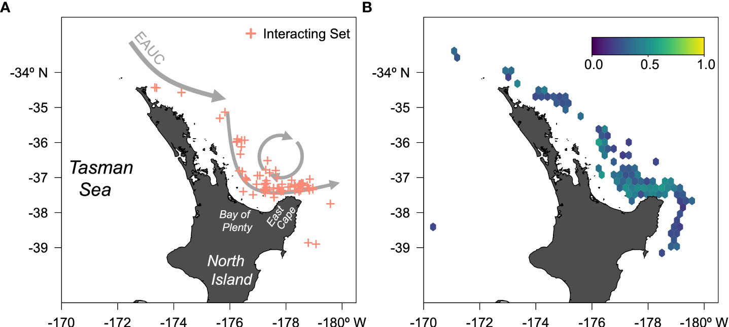
Figure 1 (A) Map of New Zealand surface longline sets from 2010 to 2021 in the first 100 days of the year and north of −42° that interacted with leatherback sea turtles. A simplified East Auckland Current (EAUC) is depicted in gray arrows. (B) Ensemble random forests predicted probability of interaction for the New Zealand surface longline from 2010 to 2021 in the first 100 Julian days and north of −42°; warmer colors indicate higher probabilities.

The increase in New Zealand leatherback sea turtle interactions is particularly challenging to manage as most appear to be either hooked in the body or flipper or entangled in the gear (Dunn et al., 2022, 2023) and the environmental drivers of the interactions encompass a wide range of the environmental space (Dunn et al., 2023). Interactions were predicted to be more likely when sea surface temperature was between 18°C and 22°C, when subsurface temperature at 200 m was between 12°C and 16°C, when northward currents were stronger (southward currents weaker), and time-varying dynamic height was less than ~2.1 (a lower heat content, possibly associated with eddy structures) (Dunn et al., 2022). In this paper, we identify key oceanographic covariates where the probability of leatherback sea turtle interactions with the New Zealand pelagic longline fleet increases and provides a means for defining areas based on the dynamic interaction–environmental response for guiding bycatch mitigation measures. In doing so, we compare two DOM informational product development schemes: simple DOM informational products consisting of single oceanographic variables (e.g., TurtleWatch) against composite products consisting of predictions of blended oceanographic covariates (e.g., South Pacific TurtleWatch or EcoCast). Simpler products likely use oceanography that fishers utilize in their own decision-making. This familiarity potentially increases understanding and model transparency. More complex products are likely to have increased model performance but run the risk of reduced transparency. These tools highlight the potential for dynamic ocean management as a bycatch mitigation strategy for reducing western Pacific leatherback sea turtle interactions with the New Zealand pelagic longline fishery within the suite of other potential bycatch mitigation strategies.

2 Methods

2.1 Fishery-dependent sampling

Following the development of domestic longlining in the early 1990s, the number of vessels in the domestic tuna fleet operating in New Zealand fisheries waters peaked in 2001 and has subsequently declined after the introduction of longline target and bycatch species into New Zealand’s Quota Management System in 2004. Since 2016, the New Zealand longline tuna fleet has consisted only of domestically owned and operated vessels (mostly between 15 and 25 m in length). The total number of longline vessels operating in New Zealand declined from 151 vessels in 2002 to 37 in 2014 and 29 in 2021. Where observers are deployed, they collect detailed information on all fish catch and protected species interactions, as well as fishing efforts and mitigation devices. On longline vessels, observers make detailed records of the fishery operation and gear types used, for example, the start and end times and locations of each fishing event, hooks per basket (basket = line between two consecutive floats), use of floats, light sticks, hook types, bait types, and snood setup. The data collected by observers are validated and uploaded to the Centralised Observer Database operated by the New Zealand Ministry for Primary Industries. In 2019, New Zealand implemented mandatory electronic catch and position reporting across the entire commercial fishing fleet. This self-reporting digital monitoring system consists of electronic catch and effort reporting and geospatial positional reporting. Commercial fishers complete, among other reports, a Non-Fish Protected Species report (for any protected species interactions) containing information on the species and quantity captured and must be completed on the day the interaction occurs. We accessed the observer and self-reporting datasets from 2010 to 2021 and linked events to remove duplicate records as the commercial fishers and observers may record the same protected species interaction event.

2.2 Ensemble random forests

To model the probability of leatherback sea turtle interaction with the New Zealand surface longline fishery, we used ensemble random forests (ERFs), which have been used previously to model rare protected species interactions that occur in longline fisheries (Siders et al., 2020). Ensemble random forests attempt to correct for the effects of successive partitioning and data sparseness that occur with rare event data (He and Garcia, 2009) by generating multiple training sets to train multiple random forests models. The resulting mean prediction across the ensemble is achieved through downsampling—balancing the majority and minority classes in a given random draw provided to a given decision tree. A variety of sampling methods have been put forth as ways to deal with the imbalance class problem in random forests (RFs) (Kuhn and Johnson, 2013), but ensemble random forests have been shown to perform well across a range of imbalances in the majority and minority classes (Siders et al., 2020).

We created the ensemble from 100 individual random forests created with 1,000 trees in each forest with five random covariates tried at each node split using the EnsembleRandomForests package in R 4.1.0 (https://zsiders.github.io/EnsembleRandomForests/index.html). We included sets with multiple interactions per set as duplicates and included the reporting type (observer-collected or fisher-reported) and the fishing effort in terms of length of the set as a covariate. Effort is included to assess if the probability of a leatherback sea turtle interaction with the New Zealand pelagic longline fishery is effort-driven. We also included environmental covariates: SST, SST anomaly, SST fronts, distance to nearest SST fronts, zonal ocean currents, meridional ocean currents, ocean current divergence, ocean current vorticity, sea-level anomaly, Okubo–Weiss parameter, eddy kinetic energy, wind speed, Ekman pumping velocity, seafloor bathymetry, distance to nearest seamount, and moon phase (see Supplementary Information for additional details on oceanographic covariate collection).

From the ERF, we calculated the variable importance of each covariate based on the mean decrease in accuracy. We used a random Gaussian noise covariate included in the model as a reference; covariates with a decrease in accuracy greater than this random variable were considered informative. Accumulated local effects (ALEs) were calculated to determine the response of the ERF model’s predicted probability of interaction to changes in values of the covariates. ALEs are the decision tree approximate of parametric response curves and employ a windowing procedure by trialing values across the covariate’s range to determine the change in the predicted probabilities from the random forest algorithm. Windowing serves to map the model’s response to a change in the covariate value akin to a marginal response curve in linear modeling. ALE does not produce a completely analogous approximation as nested interactions between covariates can be difficult to untangle.

We ran an initial ERF including Julian day among the covariate set and used the accumulated local effects plot of Julian day to subset the dataset to time of the year with more than 75% of the interactions. The ERF was rerun using this subsetted dataset to re-estimate the environment–interaction relationships without the confounding Julian day effect. Ensemble predictions from the individual random forests predicted the probability of interaction for each fishery set by averaging across the ensemble. We assessed the ensemble model performance using threshold-free metrics: area under the curve, root mean squared error, and true skill statistic. We also calculated threshold-dependent metrics of the true positive rate (specificity), the true negative rate (sensitivity), and the correlation coefficient using the maximum sensitivity and specificity threshold.

2.3 Hindcast assessment

To assess the performance of both the full model and individual environmental covariates for defining areas for fishers to avoid, we picked the five environmental covariates with the highest variable importance as potential candidates for defining areas of avoidance. This was done to simplify the suite of parameters needed for prediction after excluding environmental covariates that fell below the variable importance of the random covariate. Areas of high interaction rate can be defined using the probability of interaction from the ERF model or as a function of the environmental variables that give rise to these probabilities. When defining areas of high interaction using environmental variables, the median ALE values (approximately spaced by the 1% quantile) were subsetted to positive values, the environmental space increasing the probability of interaction, and we identified the maximum value in this range. We then iteratively expanded around the maximum based on whether the ALE response was lower to the left or right of the existing envelope. This was done because ALE values can decrease unidirectionally from the maximum value or decrease on either side (dome-shaped) (see Figure 2—inset). For each envelope, we determined the range of environmental space encompassed in the envelope and the proportion of the total positive ALE response volume filled by each envelope. To define areas using ERF-predicted probabilities, probability ranges were selected from an upper percentile of 100% and varying the lower percentile, from 5% to 95%. The effect is that each area defined by these percentiles ranges from the top 95% of values to the top 5% of values.

Figure 2

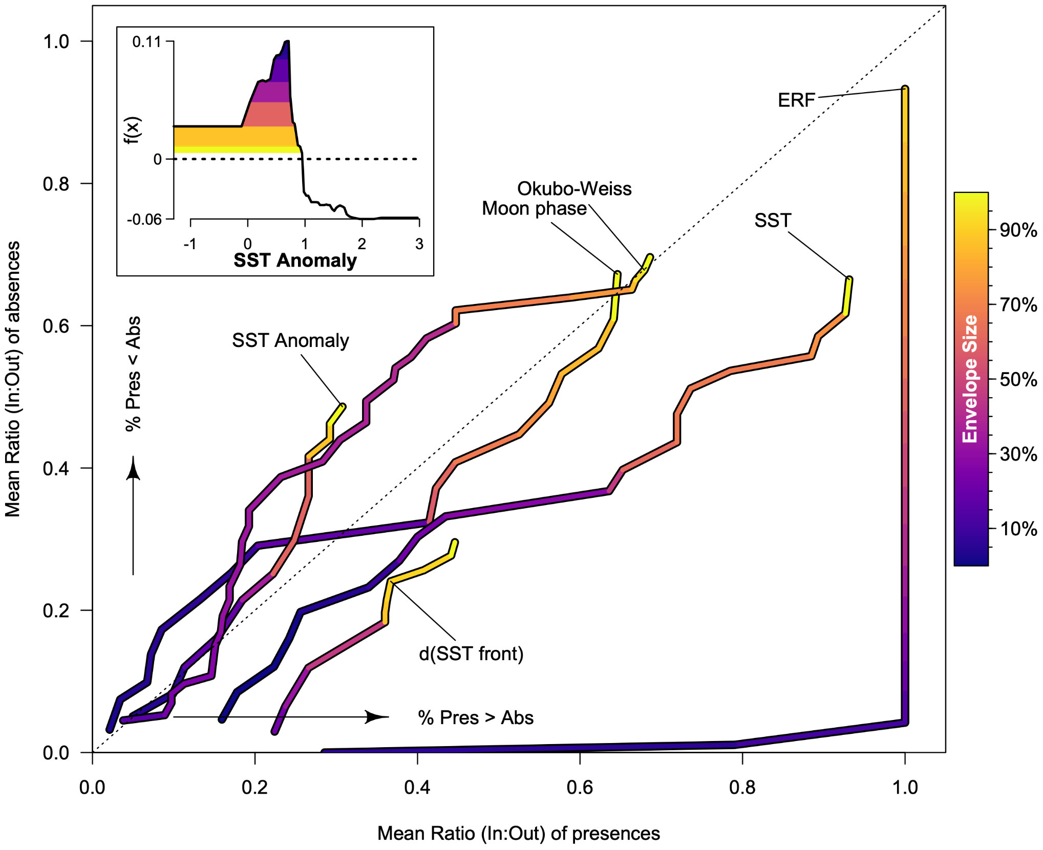
Figure 2 Hindcast performance of the top 5 environmental covariates and the composite ensemble random forest (ERF) prediction in terms of the ratio of presences and absences in and out of the covariate/prediction envelope. Warmer colors indicate wider covariate/prediction ranges and larger covariate/prediction envelopes. Lines further to the right and below the 1:1 dotted line indicate an envelope that effectively discriminates between presences and absences. Inset is the SST anomaly accumulated local effects plot with the respective envelopes shown in the filled regions, and each larger envelope (warmer colors) subsumes the smaller envelopes.

We assessed three aspects of areas identified by individual environmental variables or the ERF that are relevant to management: how effective the variable or ERF was at identifying areas with and without bycatch, whether the areas identified are spatially coherent and therefore more easily enforceable in real-world management, and the proportion of the total fishing area identified. To create a metric of discrimination for each envelope defined by an individual environmental covariate or the ERF-predicted probability of interaction, we calculated the ratio of the number of interacting sets (presences) and non-interacting sets (absences) in and out of the envelope space by year; a high ratio indicates that the covariate or ERF is effective at identifying which sets have bycatch while minimizing the inclusion of sets without bycatch. To understand the clustering of sets within an envelope, a measure of spatial coherence, as well as the envelope’s footprint, we calculated the global Moran’s I statistic using the spdep package for each year and each covariate (Bivand and Wong, 2018). We also calculated the proportion of the area occupied by sets in each envelope in each year to the total area occupied by all sets across all years, i.e., the total fishery footprint. From these yearly metrics, we calculated the mean and standard deviation across years for each envelope as well as the correlation of the mean and standard deviation with the envelope size for each covariate and each metric. To understand how different covariates or ERF-defined envelopes traded off between the range of envelope, the ratio of interacting and non-interacting sets in and out of the envelope, the clustering of the sets in the envelope, and the proportion of the total fishing area in the envelope, we rescaled the proportional area and the global Moran’s I metrics to be between 0 and 1 and added all the aforementioned metrics together for each envelope. We then identified potential envelopes that performed best across all metrics.

Lastly, we used the best-performing envelope (covariate- or ERF-defined) to hindcast, at several envelope sizes, the spatial area of the envelopes in the fishery operational area. We generated a hexagonal grid over the fishery area with cells roughly 1,700 km² and used the oceanographic covariate extraction routine to generate values for the whole grid (see Supplementary Information for additional details). For time points, we extracted the oceanographic covariates across the grid every 7 days, starting on January 1, for the first 14 weeks of the year to nearly cover the first 100 days of the fishing season for the last 3 years of fishing data, 2019–2021. We specified the grid cell size to be larger than the spatial resolution of the coarsest oceanographic covariate and used a week time frame to integrate across the various temporal resolutions of the oceanographic products (see Supplementary Information for additional details on resolution). We then predicted the ERF onto these covariates to generate a probability of interaction field. To define the spatial area of the envelope, we determined the threshold of probability of presence that corresponded to the covariate- or ERF-defined quantiles. We used this threshold to turn the continuous probability of interaction into binary predictions and visualized the resulting spatial areas of the various envelopes.

3 Results

3.1 Fishery-dependent samples

Fishery-dependent data were obtained from 5,677 surface longline sets between 2010 and 2021. This included 2,195 sets from self-reporting vessels and 3,482 observed sets. Leatherback sea turtle interactions were reported in 116 sets, involving a total of 146 turtles; 5,561 sets had no interactions. Of the 116 sets with interactions, 93 interacted with one turtle, 18 with two turtles, three with three turtles, and two with four turtles. Of the 5,677 sets, 5,520 could be matched with oceanographic covariates. Sets that could not be matched were generally the result of errors in geopositioning. This matched dataset covered 138 of the 146 leatherback sea turtle interactions. Three-quarters of the total leatherback sea turtle interactions were north of −42° and occurred in the first 100 Julian days of the year. Subsetting the data down to this time period resulted in 841 (38.3%) of the self-reported sets and 425 (12.2%) of the observed sets being used in the ERF model covering 110 leatherback sea turtle interactions.

3.2 Ensemble random forests

Threshold-free performance metrics for the ERF indicate good model performance: the area under the curve was 0.998, the true skill statistic was 0.982, and the root mean squared error was 0.321 (Table 1). The maximum sensitivity and specificity threshold was 0.616 resulting in a 99.1% true positive rate (108/109), a 98.2% true negative rate (1,080/1,100), a 1.7% false positive rate (20/1,100), and a 0.9% false negative rate (1/109) (Table 1). Predicted probabilities of interaction were low to moderate, with higher probabilities concentrated around the north coast of East Cape in the Bay of Plenty (Figure 1). The variables that were above the random Gaussian noise reference were, in order of importance, Okubo–Weiss, SST anomaly, SST, moon phase, distance to SST front, chlorophyll-a, sea-level anomaly, meridional ocean currents, and eddy kinetic energy (Figure 3). Eight other environmental covariates (SST fronts, zonal ocean currents, ocean current divergence, ocean current vorticity, wind speed, Ekman pumping velocity, seafloor bathymetry, distance to nearest seamount) as well as the fishery effort and reporting covariates fell below the random Gaussian noise reference.

Table 1

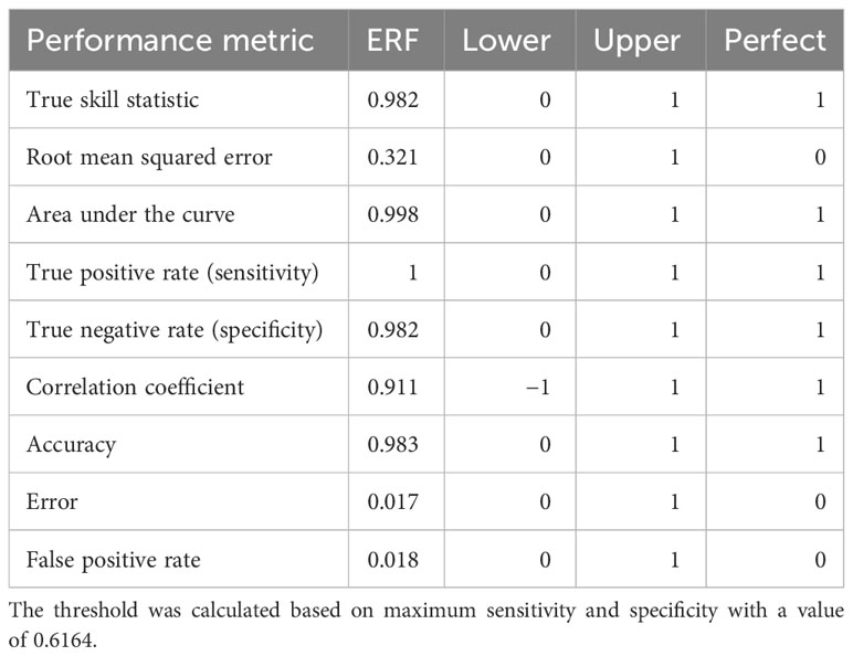
Table 1 Ensemble random forest threshold-free and threshold-dependent performance metrics with the lower and upper bounds of a given metric as well as the value under perfect classification.

Figure 3

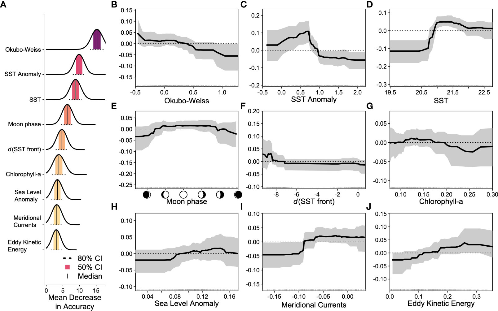
Figure 3 (A) Variable importance measured by mean decrease in accuracy for the top 9 environmental covariates in the ensemble random forests model with darker colors indicating higher importance; the shaded region is the 50% confidence interval, while the dashed line indicates the 80% confidence interval from across 100 forests in the ensemble. (B–J) Accumulated local effect plots for the top 9 environmental covariates indicating the change in model prediction (y-axis) as a function of the change in the covariate (x-axis). The solid line indicates the median relationship, and the gray-shaded region indicates the 80% confidence interval across 100 forests in the ensemble.

3.3 Hindcast assessment

Comparing hindcast discrimination performance using the top 5 oceanographic covariates, only SST and distance to SST front accrued more interacting sets than non-interacting sets as the envelope size increased (Figure 2). Okubo–Weiss, SST anomaly, and moon phase initially had an equal amount of interacting sets and non-interacting sets. Okubo–Weiss and SST anomaly shifted to accumulating more non-interacting sets than interacting sets after the envelope exceeded 10% of the maximum size, while moon phase shifted approximately 20% of the maximum envelope to accumulating more interacting sets than non-interacting sets. At the maximum envelope size, the Okubo–Weiss parameter had nearly equal ratios of interacting and non-interacting sets in and out of the envelope (69% and 70%, respectively), SST anomaly had a higher ratio of non-interacting sets (49%) than interacting sets (31%), moon phase had similar ratios (64% interacting, 67% non-interacting), and SST had a higher ratio of interacting sets (93%) than non-interacting sets (67%), as did distance to SST front (44% interacting, 30% non-interacting). The envelopes conditioned on the ERF probability of presence outperformed all single oceanographic covariate envelopes at small envelope sizes with the ability to encompass up to 100% of interacting sets while only accumulating 4.2% of absences when the envelope accumulated 15% of the probability values (Figure 2). After this point, further increases in the ERF probability of presence envelope only increased the percentage of absences until at the maximum envelope size (95% of the distribution of possible probabilities); there was a ratio of 93.3% of non-interacting sets in and out of the envelope.

Not surprisingly, as envelope size increased, so did the mean proportional area ($\rho$ between 0.11 and 0.95, Table 2) occupied by sets in the envelope with the largest envelopes occupying between 0.4% (ERF) and 26% (Okubo–Weiss) of the total fishing area (Supplementary Figure 1A). The mean spatial coherence, measured by global Moran’s I, behaved somewhat differently ($\rho$ between −0.46 and 0.91, Table 2) with the most clustering in sets occurring generally at larger envelope sizes but only at the maximum size for SST, ranging between 5% (ERF) and 88% (distance to SST front) for the other covariates. Overall, the mean proportional area and global Moran’s I were moderately positively correlated for all covariates except for SST anomaly and SST, which were strongly positively correlated, and the ERF, which was moderately negatively correlated (Supplementary Figure 1A) (Table 2). However, there was considerable interannual variability in the proportional area occupied and the global Moran’s I (Supplementary Figure 1B). With the exception of moon phase ($\rho$ = −0.56), variability in the proportional area strongly positively correlated ($\rho$ > 0.65) with envelope size, while variability in global Moran’s I strongly positively correlated with envelope size for SST anomaly, SST, and moon phase; weakly positively correlated for distance to SST front; weakly negatively correlated for Okubo–Weiss; and not correlated for the ERF (Table 2) (Supplementary Figure 1B).

Table 2

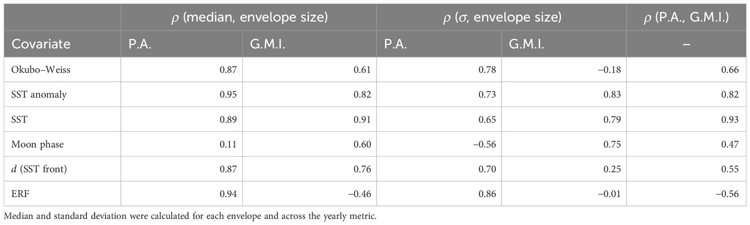
Table 2 Correlation (ρ) of the median and standard deviation with envelope size for the proportional area (P.A.) and the global Moran’s I statistic (G.M.I.) as well as the correlation between the median proportional area and the global Moran’s I statistic.

When seeking to maximize the ratio of interacting sets inside versus outside of the envelope, maximize the ratio of non-interacting sets outside versus inside of the envelope, minimize the proportional area, and maximize the global Moran’s I, the ERF-defined envelopes outperform all other envelopes until the envelope sizes exceed 65% (Figure 4). At this point, the SST-defined envelopes do better than the ERF envelopes as the SST envelopes are more clustered and occupy a smaller area. The Okubo–Weiss parameter, the top oceanographic covariate identified by ERF, performs the second best when envelope sizes are less than 25% then falls sharply to the worst performing at larger envelope sizes. At small envelope sizes, SST anomaly, SST, moon phase, and distance to the SST front all perform similarly then spread apart between envelope sizes greater than 15% and less than 80% before all except SST converge back to similar performance (Figure 4). The top-ranked envelope was the ERF-defined envelope at an envelope size of 15% (corresponding to the probability of interactions greater than 54%) as this envelope encompassed 100% of interacting sets in the hindcast assessment and 4% of non-interacting sets, and this had a minimal footprint but was weakly clustered.

Figure 4

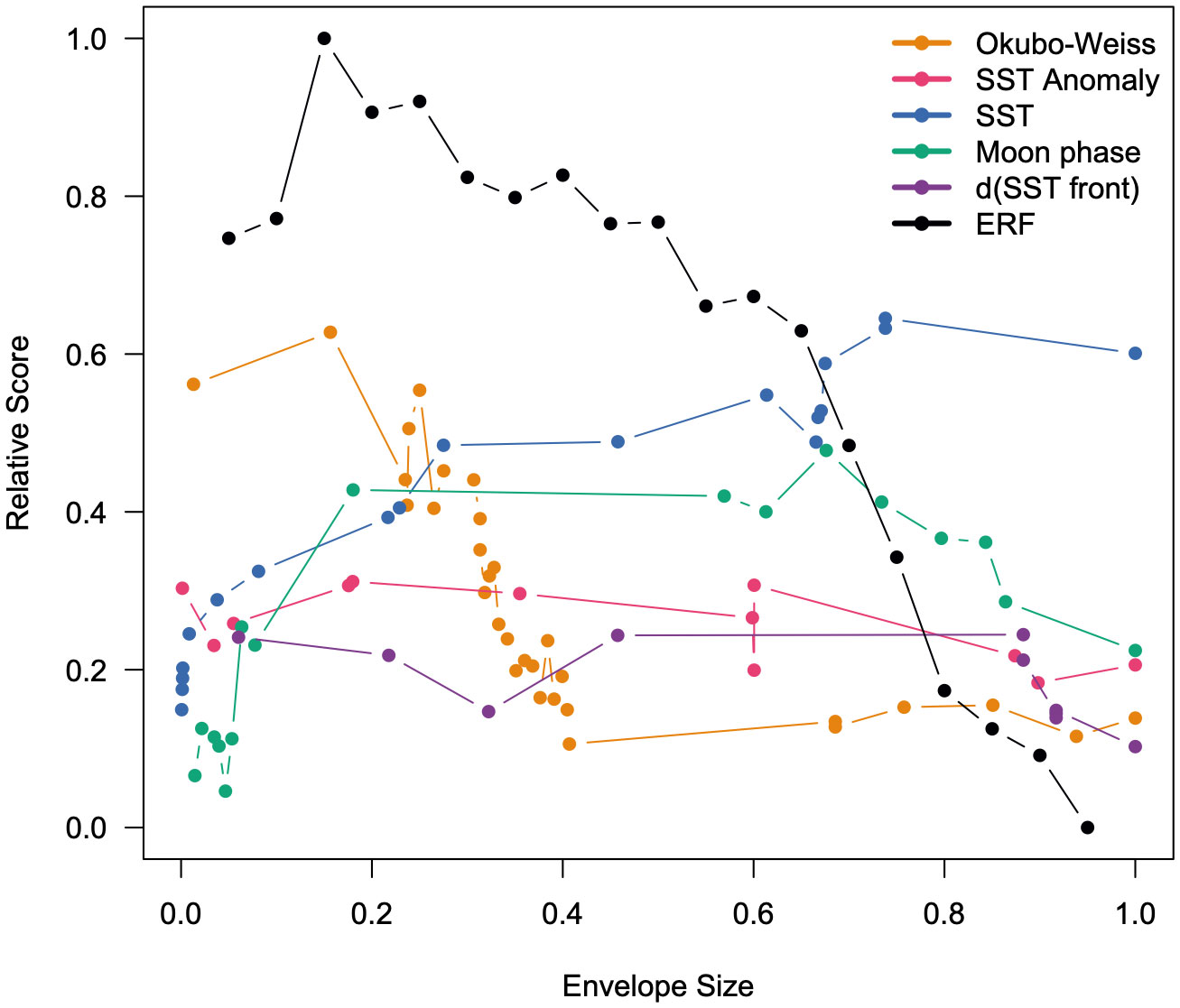
Figure 4 Relative optimization score of each oceanographic covariate- or ERF-defined envelope as a function of envelope size when seeking to maximize the ratio of interacting sets inside versus outside of the envelope, maximizing the ratio of non-interacting sets outside versus inside of the envelope, minimizing the proportional area, and maximizing the global Moran’s I.

Using the ERF-defined envelope, we hindcast-predicted onto the first 14 weeks of oceanographic covariates for the last 3 years (2019–2021) to visualize the spatial areas of the envelopes (Figure 5). We considered the most optimal envelope first, the 85th percentile of ERF probability of interaction predictions and corresponding to a threshold cutoff of 0.52 (Figure 4). We then considered other well-performing ERF-defined envelopes at the 75th, 65th, and 55th percentiles corresponding to threshold cutoffs of 0.42, 0.35, and 0.31, respectively (Figure 4). The effect of lowering the percentile (and corresponding cutoff value) generally increased the spatial footprint of the envelope (Figure 5). On average, over the 42 weeks predicted over, the 85th percentile covered 0.17% of the cells, the 75th covered 2.6%, the 65th covered 9.9%, and the 55th covered 19.8%. In some weekly predictions, the 55th percentile envelope area covered over a third of the cells. These values increase when we subset to just cells where the fishery has historically fished at least once from 2010 to 2021; the 85th percentile covered 0.7% of the cells, the 75th covered 5.2%, the 65th covered 15.2%, and the 55th covered 26.7%. Again, in some weekly predictions, the 55th percentile envelope area covered nearly half of the historic fishing area (48.9%, Figure 5S) but also could cover as little as 2% (Figure 5H). The coefficient of variations across the 42 weekly predictions decreased as the envelope area increased with the 85th percentile having a CV of 141%, the 75th having a CV of 86%, the 65th having a CV of 65%, and the 55th having a CV of 48%. Generally, by late January and to late March, the 65th percentile or above envelopes encompassed the north coast of East Cape (Figures 5C-G, J-N, P-U), the area also identified as having a high probability of interaction across the fishery dataset (Figure 1B). However, these hindcast predictions also highlighted areas northwest of North Island in the Tasman Sea (see Figure 5E for a representative example) but also down along the west coast of North Island (Figures 5K, G, S). Very little fishing effort and no leatherback sea turtle interactions were present in these areas in our dataset (Figure 1A).

Figure 5

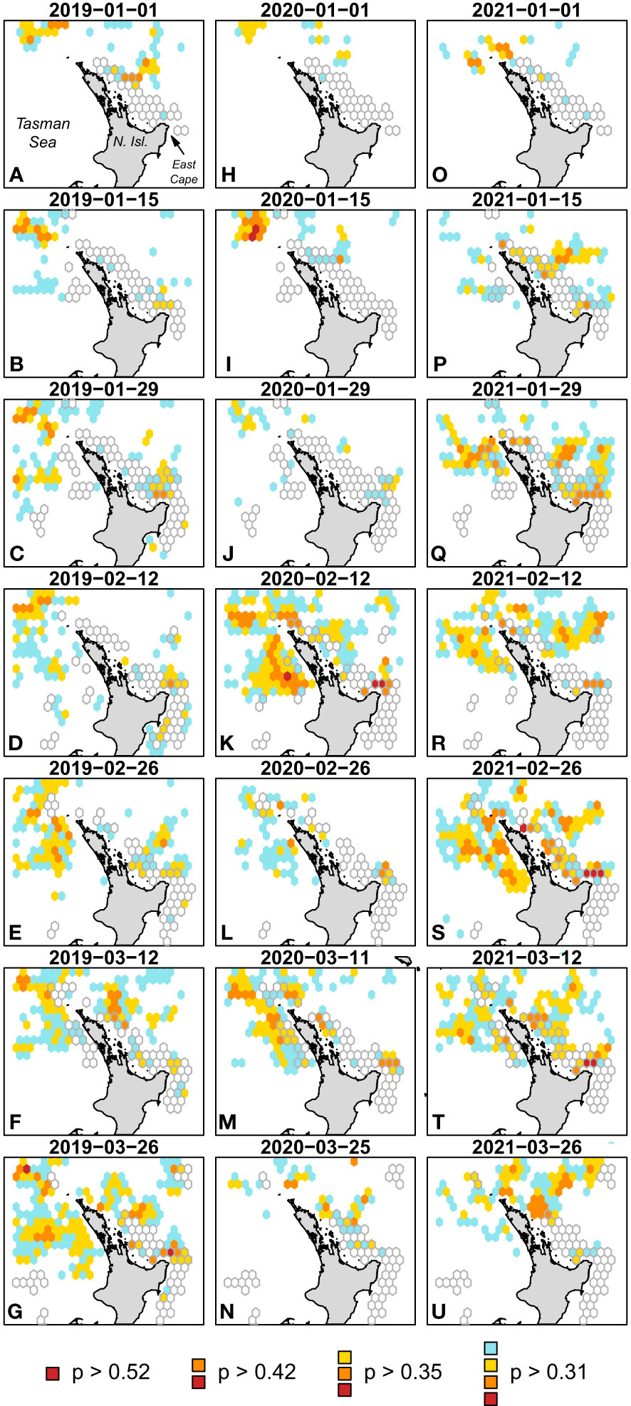
Figure 5 Fortnightly predicted envelopes from the ensemble random forest predictions to environmental conditions in 7 weeks in 2019 (A–G), 2020 (H–N), and 2021 (O–U). Envelopes were defined as predictions over the 85th (p > 0.52), 75th (p > 0.42), 65th (p > 0.35), and 55th (p > 0.31) percentiles. Gray bordered cells indicate the fishing area with at least three sets from 2010 to 2021 during the corresponding week of the year of the predicted envelopes.

4 Discussion

Substantial increases in the bycatch interactions with Critically Endangered western Pacific leatherback sea turtles in the New Zealand pelagic longline fishery necessitate the exploration of bycatch mitigation strategies (Dunn et al., 2023). We compared a series of environmentally-defined dynamic ocean management informational tools to inform a spatiotemporal bycatch mitigation strategy. Our ensemble random forests model was highly effective at discriminating between interacting and non-interacting sets using a suite of oceanographic covariates aligned to the fishery-dependent data. Using this model to assess management strategies by incorporating measures of discrimination, spatial coherence, and spatial footprint, the ERF predictions outperformed the top 5 environmental covariates in both predictive capacity and management efficiency. However, the ERF model resulted in a more complex mosaic of potential spatiotemporal closures that could complicate implementation. Nonetheless, our framework could be used to inform future management in the area provided that the dissemination of such information to fishers can be done in a viable way.

Overall, our results illustrate that DOM informational products made of composite features outperform those made of simple features across a variety of metrics. Other DOM informational products have found similar results. The South Pacific TurtleWatch informational product used a suite of static and dynamic oceanographic features to define their linear model-based predictions, such as bathymetry, sea surface temperature, frontal probability index, and sea surface height (Hoover et al., 2019). EcoCast used a wider set of static, temporally dynamic, and spatiotemporally dynamic oceanographic features along with a machine learning approach to develop three bycatch risk surfaces that are then combined through weighting schemes for an informational product that identifies bycatch risk across multiple species (Hazen et al., 2018). These composite approaches stand in stark contrast to TurtleWatch, which relied on sea surface temperature as a more easily measured and communicated proxy variable for high chlorophyll-a concentrations associated with the North Pacific Transition Zone (Howell et al., 2008). While DOM informational products like South Pacific TurtleWatch, EcoCast, and the ERF predictions here have high discriminatory ability and achieve specificity, there has not been a validation of their predictive ability nor their implementation success as an informational product. Even simpler products such as TurtleWatch do not appear to be readily used by fishers (Siders et al., 2023). It is challenging to identify whether the incentive structures, dissemination, or generality are to blame. Nonetheless, the key hurdles identified by Lewison et al. (2015) of regulatory frameworks and incentive structures, technological and analytical requirements, and stakeholder participation remain challenges to the implementation of DOM as a bycatch mitigation strategy.

DOM informational products are still useful. Our approach identified that much of the fishing grounds had some risk of leatherback sea turtle interactions in any given year; however, we also identified scattered smaller areas along or seaward of the continental margin of the Bay of Plenty where the ERF-predicted interaction probability is the highest (Figure 1B). This area was noted by Dunn et al. (2023) and marks the southern margin of the East Cape Eddy, a large permanent warm core eddy formed by the East Auckland Current (Chiswell and Roemmich, 1998) (Figure 1A). The zooplankton assemblages of this eddy are dominated by salps, consistent with the high predicted occurrence of leatherback sea turtles in this area (Bradford and Chapman, 1988). Potential mitigation strategies include disseminating these smaller areas to fishers as potential leatherback sea turtle interaction hotspots for voluntary avoidance, or as closures in particularly high interaction years, or instituting move-on rules when interactions occur in this area. Move-on rules are a dynamic strategy whereby fishers are directed a certain distance away from an area for a period of time after observed or reported bycatch (Dunn et al., 2014). Move-on rules may be implemented by government agencies or private groups (e.g., NGOs, fisher collectives), can vary in temporal and spatial extent (Little et al., 2015; Dunn et al., 2016), and more effectively reduce bycatch while also limiting target catch reductions when used at fine spatiotemporal resolutions (e.g., daily,<20 km²) (Dunn et al., 2016). The 85th percentile envelope spatial areas are typically only predicted to last 2 weeks and in one or two grid cells (Figure 5). This small spatiotemporal extent of high probability areas of leatherback sea turtle interaction indicates that pairing a DOM-defined spatiotemporal area with a move-on rule may be effective in New Zealand.

Providing metrics that identify the tradeoffs inherent in any DOM-based bycatch mitigation strategy is critical in any tool. Metrics of fishery impacts (proportions of interacting and non-interacting sets) and management tradeoffs (spatial coherence and spatial footprint) provide a means to decide between potential strategies. Envelope size is a key implementation decision because of the tradeoff between a reduction in false negatives (observed interactions but predicted non-interactions) and the generation of false positives (observed non-interaction and predicted interaction) as envelope size increases (Figure 2). Interestingly, this tradeoff varied considerably among the top 5 environmental covariates we explored. Some covariates had the same slope as envelope size increased (distance to SST front and SST anomaly), while others behaved differently as the envelope size increased (moon phase, SST, and Okubo–Weiss). This variability in some covariates is another important consideration to make when choosing between covariates used to define areas, particularly when relying on single covariate products.

As a salient example, small SST envelopes encompassed more absences than presences but rapidly encompassed more presences than absences as the envelope expanded from 20.95–21.57°C to 20.95–21.76°C (Figure 2). This 0.19°C increase shows that even minor changes can lead to massive differences in performance. It is worth noting that this very small change in SST is very difficult to implement as this is close to the level of precision for the satellite product and below the level of precision for on-vessel sensors. This precision issue lends weight toward providing georeferenced real-time composite products rather than single covariate environmentally defined areas. In our case, the composite product outperforms all of the single oceanographic variable products, but for other fisheries, this may not be the case (Free et al., 2023). More recent DOM products implement complex analytical regimes to develop composite risk surfaces that are not compared with simpler approaches (Hazen et al., 2018; Hoover et al., 2019). This approach emphasizes discrimination-based performance over implementation-based performance. To truly evaluate a DOM product’s performance, it is likely that some metrics we included in our optimization need to be factored in. Additional metrics are also likely needed such as manager- and/or fisher-defined weights based on ease of use, real-time capability, or simplicity. There is likely an unidentified tipping point where a more complex model/strategy could be a more effective mitigation strategy, but participation is so low that the realized efficacy of the method is lower. For DOM to be an effective mitigation strategy, it is necessary for the analytical components to more fully integrate management tradeoffs (Free et al., 2023) and, likely, move to a management strategy evaluation approach.

This New Zealand pelagic longline bycatch case study highlights the potential benefits and limitations of DOM-based bycatch mitigation strategies. The inherent dynamism and complexity of pelagic fisheries and their interactions with protected species have also tended to produce complex DOM informational products. As a result, it can be difficult to transform the model output into implementable discrete areas for closures or avoidance and communicate specifically why a particular area is identified (Free et al., 2023). Inherent to the development of DOM-based bycatch mitigation tools is a modeling effort that produces a great deal of information that can guide new management strategies. This information can include determining whether interactions are effort-driven, identifying environment–interaction relationships, and testing a variety of informational product styles. We recommend that this information be used to develop more nuanced bycatch mitigation strategies generally. Patterns highlighted by the modeling process can be used for discerning whether gear or fishing behavior mitigation is needed when interactions are effort-driven, spatiotemporal mitigation when high interaction areas are clearly discriminable, move-on rules when DOM strategies may be difficult to implement, or pairing strategies to address the challenge of rare protected species bycatch interactions.

Data availability statement

The underlying fisheries-dependent datasets are not available for public dissemination due to confidentiality requirements. The raw turtle capture and fishery catch and effort data supporting the conclusions of this article can be obtained from the New Zealand Ministry of Primary Industries and Department of Conservation. Requests to access the datasets should be directed to Charity.Puloka@mpi.govt.nz.

Author contributions

ZS: Data curation, Formal Analysis, Investigation, Methodology, Visualization, Writing – original draft, Writing – review & editing. CM: Data curation, Project administration, Validation, Writing – original draft, Writing – review & editing. CP: Data curation, Project administration, Resources, Validation, Writing – original draft, Writing – review & editing. SH: Conceptualization, Data curation, Resources, Supervision, Validation, Writing – original draft, Writing – review & editing. CD: Investigation, Validation, Writing – original draft, Writing – review & editing. CL: Investigation, Methodology, Visualization, Writing – original draft, Writing – review & editing. RA: Conceptualization, Investigation, Methodology, Resources, Writing – original draft, Writing – review & editing. TJ: Conceptualization, Funding acquisition, Resources, Supervision, Writing – original draft, Writing – review & editing.

Funding

The author(s) declare financial support was received for the research, authorship, and/or publication of this article. Funding was provided through award NA21NMF4720548 by the National Marine Fisheries Service.

Acknowledgments

We would like to acknowledge Robert Gear, Dominic Vallieres, Heather Benko, and Sonja Austin for facilitating this collaboration. We would also like to thank the fishers and observers who provided the fisheries-dependent sampling used herein. We would like to thank the two reviewers for their helpful comments and feedback.

Conflict of interest

The authors declare that the research was conducted in the absence of any commercial or financial relationships that could be construed as a potential conflict of interest.

Publisher’s note

All claims expressed in this article are solely those of the authors and do not necessarily represent those of their affiliated organizations, or those of the publisher, the editors and the reviewers. Any product that may be evaluated in this article, or claim that may be made by its manufacturer, is not guaranteed or endorsed by the publisher.

Supplementary material

The Supplementary Material for this article can be found online at: https://www.frontiersin.org/articles/10.3389/fmars.2024.1342475/full#supplementary-material

References

Abraham E. R., Tremblay-Boyer L., Berkenbusch K. (2021). Estimated captures of New Zealand fur seal, common dolphin, and turtles in New Zealand commercial fisheries, to 2017–18. New Zealand Aquatic Environment and Biodiversity Report No. 258. (Wellington, NZ: Fisheries New Zealand), 94.

Google Scholar

Allen S. D., Gough A. (2006). Monitoring environmental justice impacts: Vietnamese-American longline fishermen adapt to the Hawaii swordfish fishery closure. Hum. Organ. 65, 319–328. doi: 10.17730/humo.65.3.bcpx6u86wc6p8dtp

CrossRef Full Text | Google Scholar

Bailey H., Fossette S., Bograd S. J., Shillinger G. L., Swithenbank A. M., Georges J.-Y., et al. (2012). Movement patterns for a critically endangered species, the leatherback turtle (Dermochelys coriacea), linked to foraging success and population status. PloS One 7, e36401. doi: 10.1371/journal.pone.0036401

PubMed Abstract | CrossRef Full Text | Google Scholar

Benson S. R., Eguchi T., Foley D. G., Forney K. A., Bailey H., Hitipeuw C., et al. (2011). Large-scale movements and high-use areas of western Pacific leatherback turtles, Dermochelys coriacea. Ecosphere 2, art84. doi: 10.1890/ES11-00053.1

CrossRef Full Text | Google Scholar

Bivand R. S., Wong D. W. S. (2018). Comparing implementations of global and local indicators of spatial association. TEST 27, 716–748. doi: 10.1007/s11749-018-0599-x

CrossRef Full Text | Google Scholar

Bradford J., Chapman B. (1988). Epipelagic zooplankton assemblages and a warm-core eddy off East Cape, New Zealand. J. plankton Res. 10, 601–619. doi: 10.1093/plankt/10.4.601

CrossRef Full Text | Google Scholar

Carretta J. V. (2021) Estimates of marine mammal, sea turtle, and seabird bycatch in the California large-mesh drift gillnet fishery: 1990-2019 (La Jolla, CA: National Oceanic and Atmospheric Administration). Available online at: https://repository.library.noaa.gov/view/noaa/33279 (Accessed June 22, 2023).

Google Scholar

Chan H. L. (2020). Economic impacts of Papahānaumokuākea Marine National Monument expansion on the Hawaii longline fishery. Mar. Policy 115, 103869. doi: 10.1016/j.marpol.2020.103869

CrossRef Full Text | Google Scholar

Chiswell S. M., Roemmich D. (1998). The East Cape Current and two eddies: A mechanism for larval retention? New Z. J. Mar. Freshw. Res. 32, 385–397. doi: 10.1080/00288330.1998.9516833

CrossRef Full Text | Google Scholar

Curtis R., Hicks R. L. (2000). The cost of sea turtle preservation: the case of Hawaii’s pelagic longliners. Am. J. Agric. Economics 82, 1191–1197. doi: 10.1111/0002-9092.00119

CrossRef Full Text | Google Scholar

Davenport J. (2017). Crying a river: how much salt-laden jelly can a leatherback turtle really eat? J. Exp. Biol. 220 (9), 155150. doi: 10.1242/jeb.155150

CrossRef Full Text | Google Scholar

Dunn D. C., Boustany A. M., Roberts J. J., Brazer E., Sanderson M., Gardner B., et al. (2014). Empirical move-on rules to inform fishing strategies: a New England case study. Fish Fish 15, 359–375. doi: 10.1111/faf.12019

CrossRef Full Text | Google Scholar

Dunn D. C., Maxwell S. M., Boustany A. M., Halpin P. N. (2016). Dynamic ocean management increases the efficiency and efficacy of fisheries management. Proc. Natl. Acad. Sci. U.S.A. 113, 668–673. doi: 10.1073/pnas.1513626113

PubMed Abstract | CrossRef Full Text | Google Scholar

Dunn M. R., Finucci B., Pinkerton M. H., Sutton P., Duffy C. A. J. (2023). Increased captures of the critically endangered leatherback turtle (Dermochelys coriacea) around New Zealand: the contribution of warming seas and fisher behavior. Front. Mar. Sci. 10. doi: 10.3389/fmars.2023.1170632

CrossRef Full Text | Google Scholar

Dunn M. R., Finucci B., Sutton P., Pinkerton M. H. (2022). Review of commercial fishing interactions with marine reptiles (Wellington, NZ: National Institute of Water & Atmospheric Research Ltd).

Google Scholar

Eckert S. A., Eckert K. L., Ponganis P., Kooyman G. L. (1989). Diving and foraging behavior of leatherback sea turtles (Dermochelys coriacea). Can. J. Zool. 67, 2834–2840. doi: 10.1139/z89-399

CrossRef Full Text | Google Scholar

Free C. M., Bellquist L. F., Forney K. A., Humberstone J., Kauer K., Lee Q., et al. (2023). Static management presents a simple solution to a dynamic fishery and conservation challenge. Biol. Conserv. 285, 110249. doi: 10.1016/j.biocon.2023.110249

CrossRef Full Text | Google Scholar

Gilman E. L. (2011). Bycatch governance and best practice mitigation technology in global tuna fisheries. Mar. Policy 35, 590–609. doi: 10.1016/j.marpol.2011.01.021

CrossRef Full Text | Google Scholar

Hays G. C., Houghton J. D. R., Isaacs C., King R. S., Lloyd C., Lovell P. (2004). First records of oceanic dive profiles for leatherback turtles, Dermochelys coriacea, indicate behavioural plasticity associated with long-distance migration. Anim. Behav. 67, 733–743. doi: 10.1016/j.anbehav.2003.08.011

CrossRef Full Text | Google Scholar

Hays G. C., Morrice M., Tromp J. J. (2023). A review of the importance of south-east Australian waters as a global hotspot for leatherback turtle foraging and entanglement threat in fisheries. Mar. Biol. 170, 74. doi: 10.1007/s00227-023-04222-3

CrossRef Full Text | Google Scholar

Hazen E. L., Scales K. L., Maxwell S. M., Briscoe D. K., Welch H., Bograd S. J., et al. (2018). A dynamic ocean management tool to reduce bycatch and support sustainable fisheries. Sci. Adv. 4. doi: 10.1126/sciadv.aar3001

CrossRef Full Text | Google Scholar

He H., Garcia E. A. (2009). Learning from imbalanced data. IEEE Trans. Knowledge Data Eng. 21, 1263–1284. doi: 10.1109/TKDE.2008.239

CrossRef Full Text | Google Scholar

Hoover A. L., Liang D., Alfaro-Shigueto J., Mangel J. C., Miller P. I., Morreale S. J., et al. (2019). Predicting residence time using a continuous-time discrete-space model of leatherback turtle satellite telemetry data. Ecosphere 10, e02644. doi: 10.1002/ecs2.2644

CrossRef Full Text | Google Scholar

Howell E. A., Hoover A., Benson S. R., Bailey H., Polovina J. J., Seminoff J. A., et al. (2015). Enhancing the TurtleWatch product for leatherback sea turtles, a dynamic habitat model for ecosystem-based management. Fisheries Oceanogr. 24, 57–68. doi: 10.1111/fog.12092

CrossRef Full Text | Google Scholar

Howell E. A., Kobayashi D. R., Parker D. M., Balazs G. H., Polovina J. J. (2008). TurtleWatch: a tool to aid in the bycatch reduction of loggerhead turtles Caretta caretta in the Hawaii-based pelagic longline fishery. Endangered Species Res. 5, 267–278. doi: 10.3354/esr00096

CrossRef Full Text | Google Scholar

James M. C., Ottensmeyer C. A., Eckert S. A., Myers R. A. (2006). Changes in diel diving patterns accompany shifts between northern foraging and southward migration in leatherback turtles. Can. J. Zool. 84, 754–765. doi: 10.1139/z06-046

CrossRef Full Text | Google Scholar

Kuhn M., Johnson K. (2013). Applied predictive modeling (New York, USA: Springer). doi: 10.1007/978-1-4614-6849-3

CrossRef Full Text | Google Scholar

Lewison R., Hobday A. J., Maxwell S., Hazen E., Hartog J. R., Dunn D. C., et al. (2015). Dynamic ocean management: identifying the critical ingredients of dynamic approaches to ocean resource management. BioScience 65, 486–498. doi: 10.1093/biosci/biv018

CrossRef Full Text | Google Scholar

Little A. S., Needle C. L., Hilborn R., Holland D. S., Marshall C. T. (2015). Real-time spatial management approaches to reduce bycatch and discards: experiences from Europe and the United States. Fish Fish 16, 576–602. doi: 10.1111/faf.12080

CrossRef Full Text | Google Scholar

Martin S. L., Siders Z. A., Eguchi T., Langseth B. J., Yau A., Baker J. D., et al. (2020). Update to Assessing the Population-level Impacts of North Pacific Loggerhead and Western Pacific Leatherback Turtle Interactions, inclusion of the Hawaii-based Deep-set and American Samoa-based Longline Fisheries (Honolulu, Hawaii: National Oceanographic and Atmospheric Adminstration). Available at: https://repository.library.noaa.gov/view/noaa/24251.

Google Scholar

Maxwell S. M., Hazen E. L., Morgan L. E., Bailey H., Lewison R. (2012). Finding balance in fisheries management. Science 336, 413–413. doi: 10.1126/science.336.6080.413-a

CrossRef Full Text | Google Scholar

NMFS and USFWS (2020). Endangered Species Act status review of the leatherback turtle (Dermochelys coriacea) (USA: Report to the National Marine Fisheries Service Office of Protected Resources and U.S. Fish and Wildlife Service).

Google Scholar

NMFS, Pacific Islands Region (2023). Endangered Species Act Section 7(a)(2) Biological Opinion Authorization of the Hawaii Deep-Set Longline Fishery (Honolulu, HI, USA: National Marine Fisheries Service).

Google Scholar

O’Keefe C. E., Cadrin S. X., Stokesbury K. D. E. (2014). Evaluating effectiveness of time/area closures, quotas/caps, and fleet communications to reduce fisheries bycatch. ICES J. Mar. Sci. 71, 1286–1297. doi: 10.1093/icesjms/fst063

CrossRef Full Text | Google Scholar

Sale A., Luschi P., Mencacci R., Lambardi P., Hughes G. R., Hays G. C., et al. (2006). Long-term monitoring of leatherback turtle diving behaviour during oceanic movements. J. Exp. Mar. Biol. Ecol. 328, 197–210. doi: 10.1016/j.jembe.2005.07.006

CrossRef Full Text | Google Scholar

Siders Z. A., Ahrens R. N. M., Martin S., Camp E. V., Gaos A. R., Wang J. H., et al. (2023). Evaluation of a long-term information tool reveals continued suitability for identifying bycatch hotspots but little effect on fisher location choice. Biol. Conserv. 279, 109912. doi: 10.1016/j.biocon.2023.109912

CrossRef Full Text | Google Scholar

Siders Z. A., Ducharme-Barth N. D., Carvalho F., Kobayashi D., Martin S. L., Raynor J., et al. (2020). Ensemble Random Forests as a tool for modeling rare occurrences. Endang Species Res. 43, 183–197. doi: 10.3354/esr01060

CrossRef Full Text | Google Scholar

Squires D., Garcia S. (2018). The least-cost biodiversity impact mitigation hierarchy with a focus on marine fisheries and bycatch issues: Least-Cost Mitigation of Biodiversity Effects. Conserv. Biol. 32, 989–997. doi: 10.1111/cobi.13155

PubMed Abstract | CrossRef Full Text | Google Scholar

Swimmer Y., Zollett E., Gutierrez A. (2020). Bycatch mitigation of protected and threatened species in tuna purse seine and longline fisheries. Endang Species Res. 43, 517–542. doi: 10.3354/esr01069

CrossRef Full Text | Google Scholar

Tapilatu R. F., Dutton P. H., Tiwari M., Wibbels T., Ferdinandus H. V., Iwanggin W. G., et al. (2013). Long-term decline of the western Pacific leatherback, Dermochelys coriacea : a globally important sea turtle population. Ecosphere 4, art25. doi: 10.1890/ES12-00348.1

CrossRef Full Text | Google Scholar

Tiwari M., Wallace B. P., Girondot M. (2013). Dermochelys coriacea (West Pacific Ocean subpopulation) (Gland, SWTZ: IUCN). doi: 10.2305/IUCN.UK.2013-2.RLTS.T46967817A46967821.en

CrossRef Full Text | Google Scholar

Wallace B. P., DiMatteo A. D., Hurley B. J., Finkbeiner E. M., Bolten A. B., Chaloupka M. Y., et al. (2010). Regional management units for marine turtles: A novel framework for prioritizing conservation and research across multiple scales. PloS One 5, e15465. doi: 10.1371/journal.pone.0015465

PubMed Abstract | CrossRef Full Text | Google Scholar

Wallace B. P., Kot C. Y., DiMatteo A. D., Lee T., Crowder L. B., Lewison R. L. (2013). Impacts of fisheries bycatch on marine turtle populations worldwide: toward conservation and research priorities. Ecosphere 4, art40. doi: 10.1890/ES12-00388.1

CrossRef Full Text | Google Scholar

Welch H., Brodie S., Jacox M. G., Bograd S. J., Hazen E. L. (2020). Decision-support tools for dynamic management. Conserv. Biol. 34, 589–599. doi: 10.1111/cobi.13417

PubMed Abstract | CrossRef Full Text | Google Scholar

Welch H., Hazen E. L., Bograd S. J., Jacox M. G., Brodie S., Robinson D., et al. (2019). Practical considerations for operationalizing dynamic management tools. J. Appl. Ecol. 56, 459–469. doi: 10.1111/1365-2664.13281

CrossRef Full Text | Google Scholar